Spatial-temporal forecasting the sunspot diagram

Abstract

Aims. We attempt to forecast the Sun’s sunspot butterfly diagram in both space (i.e. in latitude) and time, instead of the usual one-dimensional time series forecasts prevalent in the scientific literature.

Methods. We use a prediction method based on the non-linear embedding of data series in high dimensions. We use this method to forecast both in latitude (space) and in time, using a full spatial-temporal series of the sunspot diagram from 1874 to 2015.

Results. The analysis of the results shows that it is indeed possible to reconstruct the overall shape and amplitude of the spatial-temporal pattern of sunspots, but that the method in its current form does not have real predictive power. We also apply a metric called structural similarity to compare the forecasted and the observed butterfly cycles, showing that this metric can be a useful addition to the usual root mean square error metric when analysing the efficiency of different prediction methods.

Conclusions. We conclude that it is in principle possible to reconstruct the full sunspot butterfly diagram for at least one cycle using this approach and that this method and others should be explored since just looking at metrics such as sunspot count number or sunspot total area coverage is too reductive given the spatial-temporal dynamical complexity of the sunspot butterfly diagram. However, more data and/or an improved approach is probably necessary to have true predictive power.

1 Introduction

Sunspots are both spatial and temporal physical phenomena visible at the surface of our Sun (and also other stars), that appear darker against the very bright background. The Sun’s surface has an average temperature of around 5780K, while by contrast sunspots have a temperature between 3000K and 4500K. This is why sunspots appear as dark spots compared to the remaining solar surface. Sunspots are created by strong concentrations of magnetic fields, these inhibit convective movements at the solar surface and this reduction in convection then reduces the temperature (see Proctor 2004, and references therein). Sunspots usually show up on the surface in pairs, each one having an opposite magnetic polarity (Hale 1908; Harvey 1999).

Records going back to 800 B.C. show that astronomers in ancient China were observing and recording sunspots (Stephenson & Arny 1980; Mossman 1989). Much later in England, an English monk named John of Worcester made the first sketch of sunspots on 8 December 1128 (Darlington et al. 1995). After the invention of the telescope in the early 1600s, observations of sunspots become more common and regular. In 1843 a German astronomer, Samuel Heinrich Schwabe, revealed the rise and fall of the yearly sunspot count; this marks the discovery of the sunspot cycle (Schwabe 1844). At first, it was thought that the sunspot cycle was strictly periodic, and Samuel Heinrich Schwabe in 1843 estimated the period to around 10 years (Schwabe 1844). Later it was found that the sunspot cycle is not periodic, or even quasi-periodic, but follows what seems to be a low dimensional chaotic oscillation (Ruzmaikin 1981; Weiss 1988, 1990; Mundt et al. 1991; Letellier et al. 2006; Spiegel 2009; Arlt & Weiss 2014), i.e. one which never repeats itself exactly. Subsequently, in 1848, Rudolph Wolf introduced the relative sunspot number, $R$, which now takes his name, confirmed Schwabe’s discovery, and through a study of daily observations of sunspots found that the average length or average period of a solar cycle was about 11 yrs. (Wolf 1852, 1859). Other measures were introduced later, such as the ‘smoothed monthly mean sunspot number’ (Waldmeier 1961; Wilson 1987, 1994). The analysis of the length of the sunspot cycle showed that this chaotic oscillation has a recurring time between 10 and 12 or so years. Interestingly, these oscillations in the mean cycle period have been associated with possible changes in the global climate (Wilson 2006; Wilson et al. 2008).

Sunspot area measurements since 1874 describe the total surface area of the Sun covered by sunspots at a given time. These measurements contain both time and latitude information (Yallop & Hohenkerk 1980; Hathaway 2015a). It is these sunspot area measurements that this article uses and analyses. Both the sunspot area coverage and the several sunspot measures show a similar low dimensional chaotic behaviour with an average period or recurring time of 11 years. These two measures, sunspot area and sunspot count, have been shown to be closely related (Wilson & Hathaway 2006), in fact to be piecewise linearly related. The area data is considered to have more physical significance because it is the sunspot area that is related to the total magnetic flux at the solar surface (Preminger & Walton 2007; Ermolli et al. 2014; McIntosh et al. 2014).

As well as the cycle itself, it was found that sunspots seems to emerge at the mid-latitudes ($\pm 35$ degrees), but as the sunspot cycle reaches a maximum (in both number of sunspots and sunspot area measures) the sunspots move to lower latitudes (Wolf 1859). Near the minimum of the cycle, sunspots appear even closer to the equator, and as a new cycle starts, sunspots again start emerging at the mid-latitudes. This pattern is called the ‘butterfly’ diagram and was first discovered by Edward Maünder and Annie Maünder in 1904 (Maunder 1904) (see also Gleissberg & Damboldt 1971, and references therein), There is also a small overlap of the two cycles, where sunspots for the new cycle emerge while the previous cycle terminates.

In addition to the low dimensional chaotic behaviour and the butterfly diagram, the sunspot cycle series have other very interesting dynamical features. The Maünder Minimum is one of them; it is the name used for the period approximately between 1645 to 1715 when sunspots became extremely rare. The term sunspot minimum was first introduced by John Eddy in a 1976 article (Eddy 1976). Other astronomers before Eddy had also named the period after Annie and Edward Maünder. This absence of sunspots was not an error due to the lack of observations or to the quality of the telescopes at the time as there was evidence for a cycle before the minimum (Wittmann 1978). Spörer noted that during one 28-year period within the Maünder Minimum (1672–1699), observations recorded fewer than 50 sunspots, much fewer than is typically observed today. A possible explanation for the coexistence of these two modes of behaviour, a weakly chaotic quasi-cycle and a switching to minima, could be that the Sun’s magnetic field is affected by intermittency (Carbonell et al. 1993; Covas & Tavakol 1997; Tavakol & Covas 1999; Polygiannakis & Moussas 1997; Covas & Tavakol 1999; Covas et al. 2001; Charbonneau 2001; Ossendrijver & Covas 2003; Charbonneau et al. 2004; Charbonneau 2005; Spiegel 2009; Deng et al. 2016) or by a two-mode switching (Weiss & Tobias 2016).

This and other earlier sunspot cycle minima are also clearly visible in the records of cosmogenic isotopes, e.g. ¹⁴C and ¹⁰Be (Beer et al. 1998), which are proxy or tracers of sunspot and/or solar activity. There is also evidence for the Maünder Minimum and possibly other minima in tree ring analysis (Stuiver 1980; Stuiver & Quay 1980; Steinhilber et al. 2012). Interestingly, the Maünder Minimum coincided with a period of lower than average European temperatures, hinting at a possible Sun–Earth climate connection (Tavakol 1978; Friis-Christensen & Lassen 1991; de Jager & Usoskin 2006; EPSNRC 2012). In addition to this possible relationship, another connection was noticed by Edward Sabine, who noted that the average period of the sunspot cycle was similar in value to the period of changes of Earth’s geomagnetic activity, giving birth to the study of solar-terrestrial connections which we now call ‘space weather’ (Sabine 1851, 1852; Suess 1979; Eddy 1983). In fact, solar activity can affect human activity in multiple ways. Solar storms can affect spacecraft electronics (Wilkinson et al. 2000; Choi et al. 2011; West et al. 2013), increase the radiation exposure for humans in space (Babayev 2003; Turner 2006; Cornélissen et al. 2009; Singh et al. 2011), affect and shut down electric grids (Kappenman 2005), and produce subtle variations in Earth’s climate (Friis-Christensen & Lassen 1991; Lassen & Friis-Christensen 1995), among others. The impact of the sunspot cycle on the climate and on geomagnetic activity, together with its direct impact on human activity makes the forecasting of the solar magnetic activity and/or the sunspot cycle of great importance.

An entire industry has been created around forecasting the sunspot cycle, using multiple methods, too many to mention in this article (for several reviews, see e.g. Hathaway et al. 1999, and references therein, and also Kremliovsky 1995; Usoskin & Mursula 2003; Pesnell 2012). These predictions or forecasting methods can be divided between pure mathematical methods (see e.g. Kane 1999; Ogurtsov 2005a, b), which ignore the physics underlying the time series, and methods based on some physical underlying mechanism (see e.g. Schatten 2005; Svalgaard et al. 2005; Dikpati et al. 2006, and references therein), using mechanisms that can explain the solar cycle such as dynamo theory (see e.g. Parker 1979, and for reviews see Ossendrijver 2003b, a). There are also techniques based on a combination of these two methods (see e.g. Hathaway & Wilson 2006; Duhau 2003).

A lot of emphasis and hard work (Schatten & Sofia 1987; Schatten et al. 1996; Layden et al. 1991; Svalgaard et al. 2005; Dikpati et al. 2006; Jiang et al. 2007; Hathaway 2009; Pishkalo 2014) has gone into forecasting the sunspot number cycle, and in particular the sunspot number at the solar cycle maximum. For the current solar cycle, which is the 24th solar cycle since counting started in 1755 and which began in late 2008 there has been an extensive body of literature trying to forecast the sunspot number at the maximum. The sunspot number at the maximum is a reductive metric, and in fact so many articles are published every year that no matter what number is calculated as the maximum, there will always be an article that matches the observed number within a reasonable error interval. This is not because of the lack of scientific value of these works, but because the maximum sunspot number over a cycle is a simplified metric, being zero-dimensional. Even the sunspot number shape across the whole of the cycle can be said to be a simplified metric as well, being one-dimensional. To make the point further, we note that the smoothed sunspot number reached a peak of 116.4 in April 2014. However, we can see from the results of the American Geophysical Union (AGU) meeting in December 2008 that there was a space filling set of forecasts, as can be seen in the ‘piano plot’ presented by W. D. Pesnell who has surveyed the scientific literature for forecasts of the cycle 24 maximum sunspot number (see Pesnell 2008, 2012). This plot illustrates that the sunspot number (or other metrics such as the average sunspot number or total sunspot area coverage) are metrics which do not seem good enough to answer the question of ‘What is the best forecasting method for sunspot activity?’ In other words, the sunspot number maximum (and the sunspot number time-series and its relatives) are functions of the total four-dimensional (three space and one time dimensional) physical data set, which are too low dimensional to be able to evaluate and compare the accuracy of different forecasting methods. Basically, important information gets lost and we cannot decide between forecasting methods.

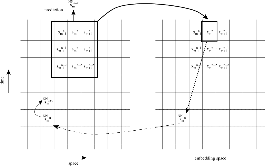
Figure 1: Representation of forecasting method. An embedding space is constructed using space and time delays, then the nearest Euclidean neighbour is found. Once found, it can be used as an approximation to deduce the next time prediction in the real space-time original space.

In this article we propose what we believe is a more general approach, by attempting to forecast the full sunspot butterfly diagram, i.e. performing a two-dimensional forecast (time versus latitude), based on the full data set for the sunspot areas and its latitudinal position, from 1874 to 2015. We use a method based on local state space reconstruction that was applied previously to spatial-temporal financial data and published with Filipe C. Mena (Covas & Mena 2011). This is, however, not the first time the forecast or reconstruction of the full sunspot butterfly space-time diagram has been attempted. Jiang et al. (2011) used the full sunspot diagram data series to uncover statistical relationships or correlations between the latitude, longitude, area, and tilt angle of sunspot groups against the cycle strength and cycle phase. Once those relationships were established, they were then able to reconstruct the sunspot butterfly diagram. The semi-synthetic reconstruction was successful for both weak and strong cycles (see their Fig. 13 and in particular Fig. 14, which shows a good match for cycle 14, a weak cycle, and cycle 19, a strong cycle). This ability to reconstruct (or forecast) both weak, medium, and strong cycles is very important and we shall come back to this point later in our own analysis. Jiang et al. (2011) also used those statistical correlations to go back in time, i.e. to recreate the sunspot diagram from 1700 to 1874, opening a very interesting research avenue now that some pre-1874 butterfly diagrams have been recovered from the full-disc drawings of the Sun for the period from 1825 to 1867 prepared by Schwabe (see Arlt & Abdolvand 2011; Arlt 2011; Arlt et al. 2013; Senthamizh Pavai et al. 2015; Leussu et al. 2016). Other data is also being recovered from historical drawings (see Arlt 2008, 2009; Usoskin et al. 2009; Diercke et al. 2015).

Later, Cameron et al. (2016) made a prediction of the future of the entire cycle 24 (see their Fig. 1). It was based on a surface flux transport model and data from synoptic magnetograms, which can be used to predict the surface magnetic field in latitude and time, and as a consequence of the relationship between sunspots and magnetic fields can be used to forecast the sunspot butterfly diagram itself. McIntosh et al. (2014) also attempted to forecast the shape of cycle 25. They used the magnetic field data to extrapolate that the first sunspots for cycle 25 will appear in late 2019 (see their Fig. 17).

Overall, we believe that by including one further dimension, it should be possible to choose between the multitude of forecasting methods. In Section 2 we describe the general method of spatial-temporal reconstruction using non-linear embeddings, and in particular the application to a two-dimensional data set (one space, one time dimension). In Section 3 we describe how the method’s parameters can be auto-calibrated using two statistical measures. In Section 4 we apply the method to the sunspot area coverage latitude-time data set and finally in Section 5 we conclude and draw on possible future research paths.

2 Method: spatial-temporal reconstruction using non-linear embeddings

Here we propose an approach which is drawn from the study of dynamical systems. Our approach is based on the embedding reconstruction of local states from chaotic dynamical systems theory applied to both the spatial and temporal components of the input series to forecast. The reconstruction preserves the dynamics under smooth coordinate transformations and the theorems by Whitney (1936), Takens (1981); Mañé (1981), and Sauer et al. (1991) guarantee the existence of the embedding. The Whitney Embedding Theorem implies that each state can be identified uniquely by a vector of $2n+1$ measurements, therefore reconstructing the phase space. The Takens Embedding Theorem refines the approach to show that the reconstruction can be reached with a single measured quantity. Takens proved that instead of $2n+1$ generic signals, the time-delayed versions of one generic signal is sufficient to recreate the $n$-dimensional manifold. Similar theoretical results were obtained in Aeyels (1981) and a more empirical account (Packard et al. 1980) was published around the same time. However, the theorems indicate an embedding dimension which is sufficient (but not necessary) and is often too high for computational purposes. In order to find more appropriate dimensions for computations we use an approach that results from a refinement of the method described by Parlitz & Merkwirth (2000) for the reconstruction of spatial-temporal time series (STTS). They applied their method successfully to both a spatial-temporal extension of the Hénon map and to the Kuramoto-Sivashinsky (KS) equation. This method was later also applied successfully to financial spatial-temporal series (yield curves) by Covas & Mena (2011), and by others to other data sets (Bialonski et al. 2015; Pan & Billings 2008; Borštnik Bračič et al. 2009; Mandelj et al. 2004, 2001).

2.1 The Parlitz-Merkwirth method

We now describe the method of Parlitz-Merwirth (Parlitz & Merkwirth 2000) of reconstructing local state data and how it can be applied to spatial-temporal data sets. Let $n=1,...,N$ and $m=1,...,M$. Consider a spatially extended time series ${\bf s}$ which can be represented by a $N\times M$ matrix with components $s^{n}_{m}\in\mathbb{R}$, which we call states of the STTS. Consider a number $2I\in\mathbb{N}$ of spatial neighbours of a given $s^{n}_{m}$ and a number $J\in\mathbb{N}$ of temporal past neighbours to $s^{n}_{m}$ (see Fig. 1). For each $s^{n}_{m}$, we define the super-state vector ${\bf x}(s^{n}_{m})$ with components given by $s^{n}_{m}$, its $2I$ spatial neighbours, and its $J$ past temporal neighbours, and with $K$ and $L$ being the spatial and temporal lags, respectively:

$${\bf x}(s^{n}_{m})=\{s^{n}_{m-IK},...,s^{n}_{m},...,s^{n}_{m+IK},s^{n-L}_{m-IK},...,s^{n-L}_{m},...,s^{n-L}_{m+IK},...\\ \cap s^{n-JL}_{m-IK},...,s^{n-JL}_{m},...,s^{n-JL}_{m+IK}\}$$ (1)

So the dimension of each ${\bf x}(s^{n}_{m})$ is

$$d=(2I+1)(J+1).$$ (2)

In their article, Parlitz-Merkwirth use only rectangular regions for the spatial-temporal neighbours of the centre element ${\bf x}(s^{n}_{m})$ in order to reconstruct ${\bf x}^{i}_{j}$. Other possible regions can be imagined, such as triangular regions (designated by lightcones). In Covas & Mena (2011) this triangular region approach was used with some success. These triangular regions try to simulate the effect of the finiteness of information transmission across space, namely that information cannot move faster than the speed of light.

Regarding boundary conditions, we follow Parlitz-Merkwirth. Owing to the boundary of the STTS, components of the local state vector ${\bf x}(s^{n}_{m})$ in (1) are not available when trying to construct states near to the STTS boundary. This problem can be overcome by extending the STTS in its spatial direction with numbers $-c$, $-2c$, $-3c$, … to the left and $+c$, $+2c$, $+3c$, … to the right. The parameter $c>0$ has to be chosen larger than the highest absolute value of the STTS. Using this construction all states close to the boundary of the STTS are located in different subspaces of the reconstruction space.

Now, for each pair $(n,m)$, there is a one-to-one invertible map $f^{-1}$:

$$f^{-1}:\mathbb{R} \to \mathbb{R}^{d}$$ (3)

$$s^{n}_{m} \to {\bf x}^{n}_{m}\equiv{\bf x}(s^{n}_{m}).$$

We now approximate $f:\mathbb{R}\to\mathbb{R}^{d}$.

Take $N_{training}$ time consecutive states $s^{n}_{m}$ of ${\bf s}$. With these states we form a training set $\mathbb{A}$ of super-states ${\bf x}^{n}_{m}$. We reconstruct a given super-state ${\bf x}^{n}_{m}\in\mathbb{A}$ by using its closest past neighbours on $\mathbb{A}$, separated in time by $\tau\in\mathbb{N}$.

We then approximate $f$ by some unknown function $F:\mathbb{R}^{d}\to\mathbb{R}$ such that

$$F(x^{n}_{m})=s^{n+\tau}_{m}.$$ (4)

There are several ways to do this. In their article, Parlitz-Merkwirth propose the following method: take a ${\bf x}^{n}_{m}$. Find the nearest neighbour to ${\bf x}^{n}_{m}$ on $\mathbb{A}$, say ${\bf x}^{i}_{j}$, in the Euclidean norm. Now, $s^{i+\tau}_{j}$, which is known a priori, will be an approximation $p^{n+\tau}_{m}$ for $s^{n+\tau}_{m}$, i.e.

$$F(x^{i}_{j})\equiv s^{i+\tau}_{j}\approx s^{n+\tau}_{m},$$ (5)

where $x^{i}_{j}$ is the nearest neighbour of $x^{n}_{m}$. We note that forecasts over longer periods of time $(\tau>1)$ can be calculated as a single large step $\tau$ or iteratively by concatenating steps with $\tau=1$.

We introduce another possible modification here with respect to the original method by considering the $n$th nearest neighbouring super-state to ${\bf x}^{n}_{m}$ and then averaging the $n$ values of $s$ obtained in this way in order to get $s^{n+\tau}_{m}$. This neighbourhood averaging also carries some weight according to the Euclidean distance to the central super-state $x^{n}_{m}$. In Covas & Mena (2011) this averaging approach was used with some success.

The embedding theorems do not state how to choose the space and time delays of the embedding. This can be done using the notion of average mutual information, which has been used widely in the past (see e.g. Abarbanel (1997); Kantz & Schreiber (1997)). This gives us an estimate for the values of the spatial and temporal delays $K$ and $L$, which can then be used to determine $I$ and $J$ and therefore the embedding dimension. Mutual information estimates how measurements of $s^{i}_{j}$ at time $i$ are connected to measurements of $s^{i+L}_{j}$ at time $i+L$.

After we calculate the (spatial and temporal) lags $K$ and $L$, we can proceed to determine the embedding parameters $I$ and $J$, for which we use the method of false neighbour detection proposed by Kennel et al. (1992) and described in detail in Abarbanel & Gollub (1996) and Abarbanel (1997). This approach calculates the number of neighbours of a point and how that number changes with increasing embedding dimension. Below the theoretical embedding dimension, many of these neighbours will be false, due to projection, but at a higher embedding dimension all neighbours are real. The advantage of using this auto-calibration as opposed to choosing those parameters based on the best match to the future observed data set is that we avoid any bias. This way the calibration is fully based on the training set and nothing else and is an unbiased approach.

3 Parameter estimation

We calibrate our parameters $I$, $J$, $K$, $L$ in equation (1) using the average mutual information first minimum (see Fraser & Swinney 1986) for the $K$ and $L$ (spatial and temporal) lags and the false neighbours method of finding the optimal embedding (spatial and temporal) dimensions $I$ and $J$ (see Parlitz & Merkwirth 2000, and references therein). In other words, we take slices in space (or in time), calculate the one-dimensional mutual information and percentage of false neighbours, and then average the values. We can then calculate an estimate for the best spatial (and temporal) lags and embeddings.

The first two parameters to calibrate are therefore the $K$ and $L$ (spatial and temporal) lags, inferred by finding the first minimum of mutual information. The mutual information is calculated as follows. Let $s^{i}$ be a one-dimensional data set and $s^{i+L}$ the related $L$-lagged data set. We note that we have to truncate the set $s^{i}$ by $L$ points in order to take into account its size when lagging it. Given a measurement $s^{i}$, the amount of information $I(L)$ is the number of bits on $s^{i+L}$, on average, that can be predicted, and is calculated as

$$I(L)=\sum_{i}\sum_{i+L}P(s^{i},s^{i+L})\log_{2}\frac{P(s^{i},s^{i+L})}{P(s^{i})P(s^{i+L})},$$ (6)

where $P(s^{i})$ is the probability of finding a time series value in the $i$-th interval and $P(s^{i},s^{i+L})$ is the joint probability of measuring $s^{i}$ and $s^{i+L}$.

Following on from Fraser and Swinney’s article (Fraser & Swinney 1986; see also Martinerie et al. 1992; Abarbanel et al. 1993), the maximum unpredictability coincides with the minimum predictability, i.e. at a minimum in the mutual information. As chaotic time series diverge exponentially, due to one or more positive Lyapunov exponents (Cencini et al. 2009), the first minimum of $I(L)$ – rather than some subsequent minimum – should probably be chosen for the time lag $L$ to sample the data.

In order to calculate the two lags for a two-dimensional set, we take slices in both space and in time, calculate the mutual information, average it, and then find the first minimum to obtain the $K$ and $L$ (spatial and temporal) lags. Once the lags are obtained, the next step in the calibration or parameter estimation is to calculate the minimum embedding dimension, or equivalently, the number of spatial and temporal neighbours to use in the phase space reconstruction. To do this, we use the method of false neighbours, as described in Kennel et al. (1992); Martinerie et al. (1992) and Abarbanel et al. (1993). This approach determines, directly from the data, when the apparent close neighbours or crossing of orbits have been eliminated by virtue of projecting the full orbit in a too low dimensional embedding phase space. The implementation by Kennel et al. (1992) is as follows. If we have an embedding in $d$ dimensions for a time series $s(n)$, and we define the distance of a phase space vector ${\bf x}(n)$ to its $r$th nearest neighbour ${\bf x}^{(r)}(n)$ by the square of the Euclidian distance,

$$R_{d}^{2}(n,r)=\sum_{i=0}^{d-1}{\left[s(n+iL)-s^{(r)}(n+iL)\right]^{2}},$$ (7)

then as we increase the dimension to $d+1$, we add a new coordinate $s(n+dL)$ to the ${\bf x}(n)$ vector. So the new distance in this $d+1$ space is

$$R_{d+1}^{2}(n,r)=R_{d}^{2}(n,r)+{\left[s(n+dL)-s^{(r)}(n+dL)\right]^{2}}.$$ (8)

If there are two false neighbours, as we increase the dimension from $d$ to $d+1$, it is expected that this distance will increase substantially. Kennel et al. define a criterion for this by designating a false neighbour as one that has

$$\sqrt{\frac{R_{d+1}^{2}(n,r)-R_{d}^{2}(n,r)}{R_{d}^{2}(n,r)}}=\frac{\left|s(n+dL)-s^{(r)}(n+dL)\right|}{R_{d}(n,r)}>R_{tol},$$ (9)

where $R_{tol}$ is some arbitrary threshold. Kennel et al. recommend using a threshold of around 10 and we use the same value later. We record and output the percentage of presumed false neighbours as a function of the embedding dimension $d$. Since we have a spatial-temporal signal, again we slice in space and in time, calculate the percentage of false neighbours, and then average over space and time as a function of $J$ and $I$, respectively.

This slicing in space and time is obviously an arbitrary choice. However, there is not – as far as we are aware – a mathematical generalisation for the calibration of the lag and dimension parameters for a multi-dimensional data series. We have not attempted in this article to explore other approaches, although we recognise that studying the stability of the embedding, and of the forecasting, as a function of the slicing and averaging methodology is an interesting research topic. A mathematical theory of mutual information in higher dimensions and a theoretically justifiable method for choosing the optimal lags and embedding dimensions in higher dimensions are sorely needed.

4 Results

4.1 Data

We analyse data for sunspot area coverage from 1874 to 2015. The data we used starts at Carrington Rotation number 275 and finishes at 2162. The data is made of blocks of 50 data points per Carrington Rotation, each point representing a latitudinal bin, all of which are distributed uniformly in $sin(\textnormal{latitude})$. The data points represent the area of that time/latitude ‘rectangle’ that is occupied by sunspot(s) in units of millionths of a hemisphere.

We take as a ‘training set’ the data from the year 1874 (i.e. the first 1646 Carrington Rotations) to approximately 1997; that is, we take as a training set the data for Carrington Rotations 275 to 1920 inclusive. We then try to forecast the sunspot area butterfly diagram from Carrington Rotation 1921 to 2162 (the latter representing approximately the year 2015); that is, we use 1646 time slices (approximately 122.92 years) to forecast the next 242 time slices (approximately 18.07 years). The training set represents approximately 12 solar cycles (cycle 11 to 22), while the ‘forecasting set’ represents approximately 1.5 cycles (cycle 23 and half of cycle 24). The entire data set, including the training set and the forecasting set, is a grid $A^{i}_{j}=A(i,j)$, with $i=1888$ and $j=50$. The training set is a grid $A(1646,50)$. The area values, in units of millionths of a hemisphere, range from 0 when there are no sunspots to the maximum value of 2580. Of the total $i\times j=94,400$ data points, approximately $27.54\%$ are non-zero, i.e. they represent a sunspot area occupying that time/latitude rectangle. For the entire data set and taking into account the points for which $A(i,j)=0$ the average is $\langle A(i,j)\rangle\approx 16.77$.

The distribution of area covered by sunspots as a function of time and latitude is by no means uniform, as can be seen in Table 1. This distribution will later influence the way we colour the real and forecasted sunspot diagram (see Figs. 6 and 7).

Table 1: Sunspot area coverage (in millionths of a hemisphere) showing the number of data points and the percentage of the total within certain area bins.

Area coverage bin	Count	Percentage of total
0	68398	72.46%
1	5790	6.13%
2	1189	1.26%
5	2105	2.23%
10	2183	2.31%
20	2555	2.71%
50	4045	4.28%
100	3362	3.56%
$\infty$	4773	5.06%

4.2 Calibration of $I$, $J$, $K$, and $L$

We first calibrate the $L$ parameter. We slice the training set into 50 (latitudinal) pure time series, and then calculate the mutual information as a function of $L$ for each of these slices. Then we average over the 50 slices, showing the average of the mutual information in order to make a decision on the optimal $L$-temporal lag.

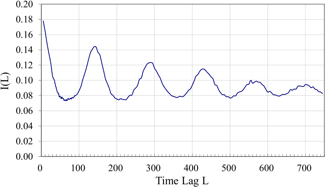
Figure 2: Average mutual information as a function of time lag $L$, $I(L)$. Although it is not clear what the exact first minimum is, due to data noise, it is close to or around $L=70$ months, which we will take as the first minimum.

We can see in Fig. 2 the usual mutual information shape for a time series, with a collection of successive local minima. We use the first minimum (Fraser & Swinney 1986; Kantz & Schreiber 1997; Cencini et al. 2009) as an indicator of the best value for the $L$-temporal lag parameter. There is clearly some noise in the figure; we note that, theoretically, the method assumes we are dealing with infinite, noise-free trajectories and there is no guarantee it will work for real physical data (Schreiber 1999). The first minimum is around $L=70$, corresponding to around 5.22 years, and we use this value hereafter. We also calculated the minima for the pure time series $A(t)=\sum_{\textnormal{latitude}}A(t,\textnormal{latitute})$, representing the total sunspot area across the entire solar disc, and we have found it to be $L=58$, corresponding to around 4.33 years or around 52 months. Zhou & Feng (2014), who have analysed the smoothed average sunspot count (as opposed to the sunspot area, but related), have arrived at a time-lag value of 38 months, while Kurths & Ruzmaikin (1990) and Mundt et al. (1991) have arrived at a value of 2-5 years and 10 months respectively. Others have found similar values (Sello 2001; Letellier et al. 2006; Jiang & Song 2011; Deng et al. 2016). For smaller daily sunspot count time series Jevtić et al. (2001) arrived at optimum time delay of 8-12 days, but we believe this is due to the effect of having both daily points and less than one solar cycle (they used around 3346 days of daily data).

In a similar way we shall calibrate the $K$ parameter. We slice the training set into 1646 (latitudinal) pure time series, and then calculate the mutual information as a function of $K$ for each one of those slices. Then we average the resulting mutual information across the 1646 slices, showing the average to make a decision on the optimal $K$-spatial lag (Fig. 3). The first minimum is around $K=9$ and we use that value thereafter.

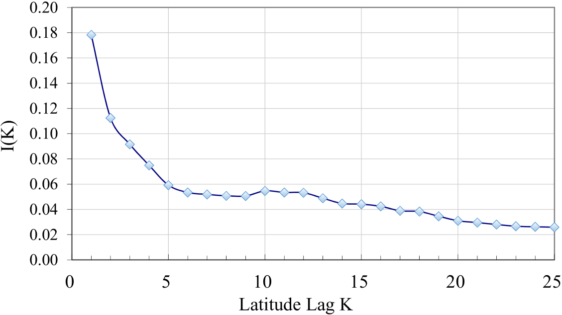
Figure 3: Average mutual information as a function of latitude grid spacing lag $K$, $I(K)$. The first minimum seems to indicate optimum latitude grid spacing of around $K=9$.

Now that we have $K=9$ and $L=70$ we can use them to create successive higher dimensional embeddings in both space and time to calculate the $I$ and $J$ optimal parameters. We take the same approach that we took for the calibration of the lags, and average the percentage of false neighbours over spatial/temporal dimensions. As indicated in Section 3, we use $R_{tol}=10$ although we tested the stability of the implied minimum embedding dimension to several values of $R_{tol}$. This can be seen in Figs. 4 and 5 as a function of $J$ and $I$, respectively.

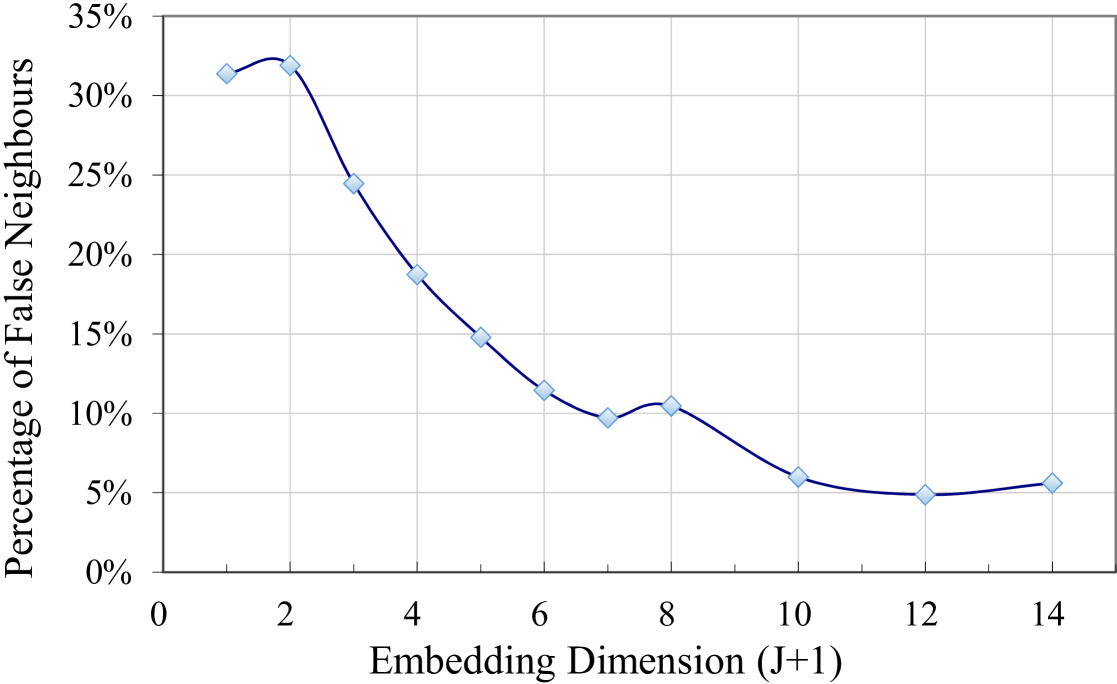
Figure 4: Percentage of false nearest neighbours averaged over all latitudes. We take the minimum embedding dimension to be the one for which the percentage is first 10% or less. The data indicates that $J+1\approx 7\implies J=6$.

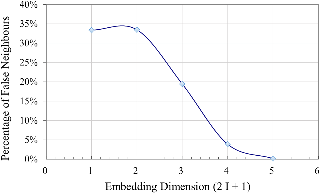
Figure 5: Percentage of false nearest neighbours averaged over all time slices. We take the minimum embedding dimension to be the one for which the percentage is first 10% or less. The data indicates that $2I+1\approx 4\implies I=2$ (we truncate $I$ as we want the embedding area to be symmetric with respect to the centre element ${\bf x}(s^{n}_{m})$).

Given the shape of the percentage of false nearest neighbours is affected by noise and the finite aspect of the time series, we take the assumption that the embedding dimension is found whenever the percentage is below 10%. The figures imply that $I=2$, $J=6$ and we use these values to attempt to forecast the sunspot diagram in the next section.

4.3 Forecast

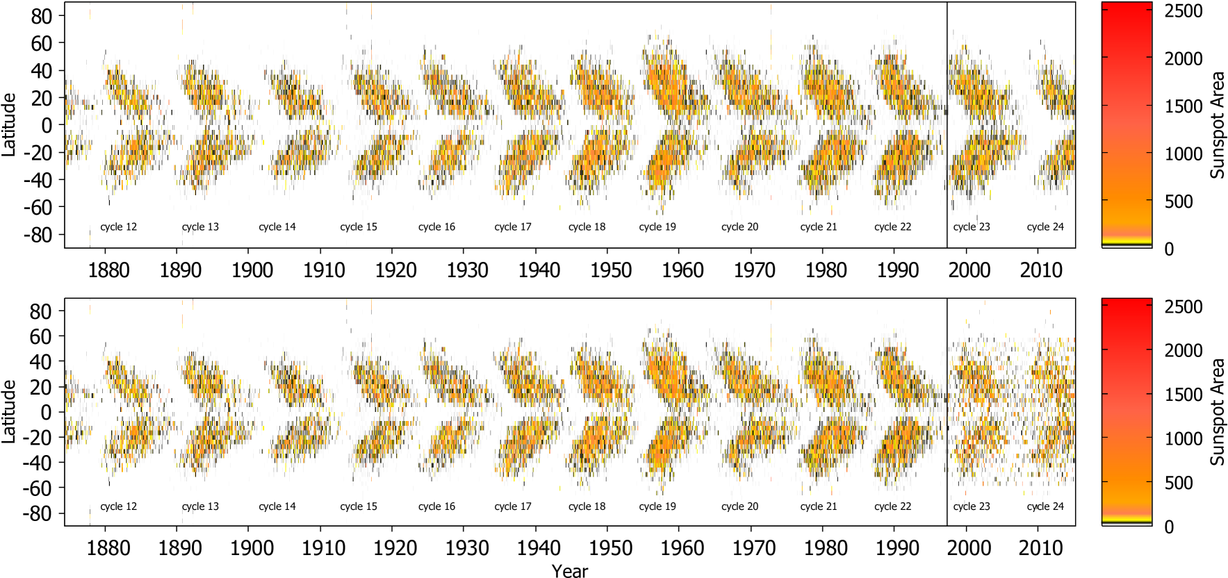
Figure 6: Spatial-temporal forecast of the last two cycles using the calibrated parameters $I=2$, $J=6$, $K=9$, and $L=70$. The top panel is the full data set, including the training set and the actual observed future data set. The bottom panel is the training set plus the forecasted set. The boundary between the training set and the forecast set is marked by a black vertical line in each plot. The main features of the butterfly diagram, namely the amplitude of the cycle and the migration to the equator, are both present, even if the forecast is far from perfect. The colour scheme used tries to follow the distribution of covered area as suggest by the data in Table 1.

Using the best parameter calibration, we have $I=2$, $J=6$, $K=9$, and $L=70$, and we now attempt to forecast approximately 1.5 cycles (cycle 23 and half of cycle 24). We forecast one data slice at a time, i.e. one Carrington rotation at a time, then concatenate, then use the same calibrated parameters to forecast the next, and so on. A total of 242 data slices are forecast in this way. The results are shown in Fig. 6 and the amplification in Fig. 7.

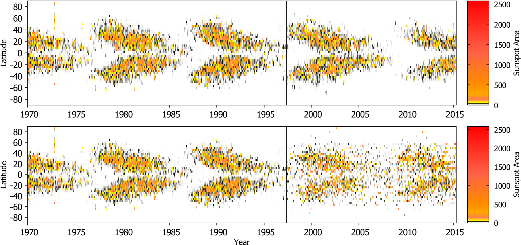
Figure 7: Amplification of the spatial-temporal forecast of the last two cycles using the calibrated parameters $I=2$, $J=6$, $K=9$, and $L=70$. The top panel is the full data set, including the training set and the actual observed future data set. The bottom panel is the training set plus the forecasted set. The boundary between the training set and the forecast set is marked by a black vertical line on each plot.

The results show that we can reproduce the two main features of the butterfly diagram; i.e. the amplitude of the cycle and the migration to the equator are both present, even if the forecast is far from perfect. There seems to be a dispersion of points in the forecast. There are also some blips, probably caused by the noise level, which may lead the algorithm to fail badly. Still overall, it is a reasonable result, considering that this particular method is generic as it does not need to know the underlying physics of the system. We also attempted to do the forecasting using the concept of lightcones, i.e. restricting the embedding vector to an isosceles triangle of data points on the original super-state vector ${\bf x}(s^{n}_{m})$ in (1), but this did not improve the forecast. We also attempted to use the weighted averaging as described in Section (2.1), but again saw no noticeable improvement. This is in contrast with the results in Covas & Mena (2011), but we have not found an explanation for this behaviour. Still by not using any modification to the auto-calibrated method, we ensure that no bias is introduced when choosing the details of the approach.

Figure 6 and the amplification in Fig. 7 show that the method works qualitatively well for both the amplitude of the cycle and the migration to the equator. Overall, the shape and angle of the latitudinal bands of the butterfly diagram seem to be preserved by the forecast. In order to put this conclusion on firmer ground, we calculated the overall sunspot area (sum over latitude) for the forecast and compared it with the observed one. These results are depicted in Fig. 8, which shows the total sunspot area, and both the original training set (and observed future set) and the forecasted set using the same parameters $I=2$, $J=6$, $K=9$, and $L=70$. Although there is quite a lot of noise (in both sets), it shows that the method seems to work at least qualitatively not only in space and time, but also on aggregated metrics such as the sum of the area over the latitude. The question of whether it really has predictive power is addressed in Section 4.5.

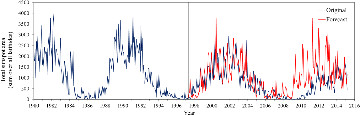
Figure 8: Overall sunspot area (sum over all latitudes) $A(t)$ and the forecast for the two last cycles using parameters $I=2$, $J=6$, $K=9$ and $L=70$. The black line marks the start of the forecast.

We also calculated the 24-point moving average

$$\overline{A(t)}\doteq\left\langle\sum_{\textnormal{latitude}}A(t,\textnormal{latitude})\right\rangle_{24}$$ (10)

to show the overall smoothed total sunspot area cycle against the original cycle. The moving average was taken backwards in time and the total sunspot area is the sum over all latitudes of $A(t,\textnormal{latitude})$. The results are depicted in Fig. 9, which shows that the method is quite good at reproducing the first cycle (cycle 23), but – not surprisingly – that it starts to fail when forecasting the next cycle (cycle 24). This could indicate that the method can only reproduce the cycle a few years ahead or – even worse – that it fails badly for weak cycles like cycle 24.

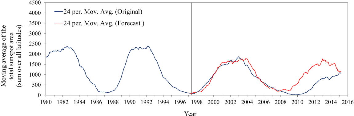
Figure 9: Moving average (24-point average) total sunspot area (sum over all latitudes) $\overline{A(t)}$ and the forecast for the two last cycles using parameters $I=2$, $J=6$, $K=9$ and $L=70$. The black line marks the start of the forecast.

4.4 Structural similarity

The method used here has the advantage of reproducing the entire spatial-temporal features of the sunspot butterfly diagram. However, it is not easy to quantitatively estimate when we have found a good forecast. The human brain is able to look at the observed butterfly diagram and the forecasted one in Fig. 6 and assess almost instantaneously whether it is a good or a bad forecast. However, using numerical quantities such as the root-mean-square error (RMSE) may not be the best way to quantify the goodness of a forecast. Although the RMSE has the advantage of being parameter free and cheap to compute, relatively simple, and memoryless, the RMSE can be evaluated at each sample independently of the other samples; it has the disadvantage of not being able to imitate the human perception of image similarity. In the particular case of the butterfly diagram, what we are after is to closely match the overall butterfly wing shape, the migration to the equator, and the overall amplitude (width and intensity).

In order to assess the similarity of the forecast with the actual sunspot butterfly diagram we use the concept of structural similarity $\textnormal{SSIM}(x,y)$ introduced by Wang et al. (2004),

$$\textnormal{SSIM}(x,y)=\frac{(2\mu_{x}\mu_{y}+c_{1})(2\sigma_{xy}+c_{2})}{(\mu_{x}^{2}+\mu_{y}^{2}+c_{1})(\sigma_{x}^{2}+\sigma_{y}^{2}+c_{2})},$$ (11)

where $\mu_{x}$ is the average of $x$, $\mu_{y}$ is the average of $y$, $\sigma_{x}^{2}$ is the variance of $x$, $\sigma_{y}^{2}$ is the variance of $y$, $\sigma_{xy}$ is the covariance of $x$ and $y$, and $c_{1}$ and $c_{2}$ are constants implicit in the structural similarity method (for details see Wang et al. 2004; Brunet et al. 2012). The SSIM index is a method for calculating the perceived quality of digital images and videos. It allows two images to be compared and provides a value of their similarity. The SSIM index is a decimal value between -1 and 1; a value of 1 is only attained in the case of two identical sets of data. The SSIM index is designed to improve on traditional methods such RMSE, which have proven to be inconsistent with human visual perception.

We use the SSIM index to measure the similarity of the forecast and the original sunspot cycle. We calculate the index using the $242\times 50$ points that are forecasted, i.e. the forecast over almost two cycles from Carrington rotation 1921. We first try to show how the RMSE metric is a bad indicator of similarity by showing the RMSE versus the SSIM for a random Monte Carlo generated collection of forecasts. We take random samples of $I=1,2$; $J=4,5,6$; $K=7,8,9$; and $L=60,\ldots,80$, together with the use of lightcones or not, and calculate the RMSE of the error (differences) between the observed and forecasted 24-point moving average of the total sunspot area $\textnormal{RMSE}(\overline{A(t)})$. This is depicted in Fig. 10 which shows first, that the auto-calibrated set of parameters we used throughout this article corresponds to a very high structural similarity index $\textnormal{SSIM}\approx 0.82790361$ which is quite good and second, it shows that for widely different forecasts, some quite good (as measured by a high SSIM) and some quite bad (low SSIM), we can have the same RMSE. We verified that these high/low SSIM values mean what they should by examining visually the forecasted sunspot butterfly diagram and comparing it with the observed one. The conclusion is that the RMSE metric is, as suspected, not a perfect and unique way way to estimate the goodness of the forecasts.

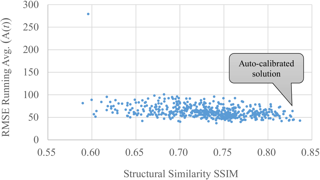
Figure 10: RMSE of the error (differences) between the observed and forecasted 24-point moving average of the total sunspot area $\overline{A(t)}$ against the structural similarity SSIM for random choices of the forecasting algorithm’s input parameters. The higher the SSIM, the closer the forecast is to the observed sunspot butterfly diagram. This shows that similar quality forecasts, at least in terms of structural similarity, can have quite different $\textnormal{RMSE}\left(\overline{A(t)}\right)$.

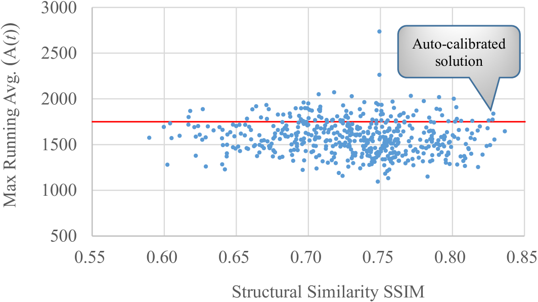
Figure 11: Maximum total sunspot area across the next forecasted cycle $\max(\overline{A(t)})$ against the structural similarity SSIM for random choices of the forecasting algorithm’s input parameters. This shows that similar quality forecasts, at least in terms of structural similarity, can have quite different maximum sunspot areas over the next cycle. The red line marks the actual real maximum of the smoothed total sunspot area across the next cycle. This clearly shows that markedly different forecasts of different quality (in space and time) can have a similar accurate maximum of the sunspot area.

The reason for the difficulties when using the RMSE is that the butterfly diagram is not really a smooth two-dimensional surface, but a very irregular data set.

Finally, as most authors try to forecast the maximum sunspot area of the next or current cycle we also examined how the forecast of the $\max(\overline{A(t)})$ over the next cycle (cycle 23) behaved against the SSIM for random samples of the calibration input parameters. These results are depicted in Fig. 11. Again, this shows that the calibration done using the first minimum of the average mutual information and the percentage of false neighbours (the above-mentioned auto-calibration) seems to work, since this one shows a $\textnormal{SSIM}\approx 0.82790361$ and a forecasted total sunspot area $\max(\overline{A(t)})$=$1774.71\text{\,}\mathrm{,}$ which is quite good given that the observed maximum of the 24-point moving average total sunspot area for cycle 23 was $1875.04\text{\,}$ This seems to show that looking at a single number (the maximum solar activity over the next cycle) may not easily differentiate between good and bad forecasts from the point of view of trying to match the full butterfly diagram.

4.5 Effectiveness of the prediction per cycle

In section 4.3 we attempted to predict cycle 23 and part of 24, using data up to cycle 22 inclusive. However, because the sunspot emergence and progression is cycle dependent (see e.g. Vitinskij 1977; Li et al. 2001, 2003; Hathaway et al. 2003; Solanki et al. 2008; Jiang et al. 2011; Ivanov & Miletsky 2011), it is quite fair to say that we may have just been lucky to reproduce cycle 23, given that it is a medium cycle. After all, the method relies on training data, and if a cycle, e.g. cycle 24, is a weak cycle, then unless the training data has visited that unusual or rarely visited part of the supposedly chaotic attractor, the forecast will inevitably fail.

To address this question of the effectiveness of the method, we ran an extra set of calculations. We looped through all the cycles and tried to forecast cycle $n$ using as the training set all cycles from the beginning (cycle 11) to $n-1$. To decide when one cycle finished and another started, we used the data in Tables 1 and 2 in Hathaway (2015b), taking for the beginning of each cycle the minimum in the 13-month running mean. This analysis should be able to answer the question of the effectiveness of the method with respect to the type of the cycle (strong/medium/weak) we are trying to predict.

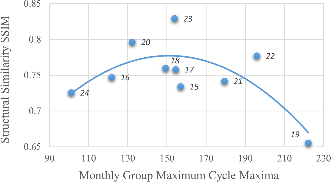
Figure 12: Structural similarity index SSIM of the forecast against the cycle strength, as given by the Monthly Group Maximum sunspot number (Hathaway 2015b). The results show that the method is most effective for medium cycles. We did not include attempts to forecast cycles 11 to 14 since the method requires enough past data, according to the auto-calibrated parameters $J$ and $L$; to forecast these cycles with this method we would need data prior to 1874.

The results of this analysis are depicted in Fig. 12, which seems to show two relationships. First, as the the number of data points increases, the predictive power of the method as measured by the SSIM index seems to improve slightly. This is as expected, as the trajectory described by the ${\bf x}(s^{n}_{m})$ embedding vectors will trace more and more the real chaotic attractor, as the time (or the size of the training set) increases. Second, the method described here seems to work better for medium cycles, as can be seen in the figure where we have superimposed a second-order fitting on the SSIM index against the strength of the cycle. In particular, for the current cycle, cycle 24, which is a weak cycle, the forecast is not that good.

The method applied here works on the basis on finding the nearest neighbour in the phase space of the embedding vectors ${\bf x}(s^{n}_{m}),$ and therefore it works better where there is a high density of neighbours. For weak and strong cycles, the theoretical attractor will be poorly traced by the embedding vectors from real data. As these are the two most extreme cases, the nearest neighbour method will be wrong more frequently. Unless more data is added, it is difficult to improve the performance of this method, a clear limitation of just using sunspot data rather than all related physical data. Several articles in the literature argue that one should use other data, e.g. geomagnetic precursors (Feynman 1982; Schatten & Sofia 1987; Thompson 1993; Hathaway et al. 1999; Hathaway & Wilson 2006; Kane 2007; Cameron & Schüssler 2007; Wang & Sheeley 2009; Ng 2016); surface magnetic fields, in particular polar fields (Schatten et al. 1978; Svalgaard et al. 2005; Muñoz-Jaramillo et al. 2013a; Petrie et al. 2014); polar faculae (Muñoz-Jaramillo et al. 2012; Muñoz-Jaramillo et al. 2013b); and even helioseismological data (Ilonidis et al. 2011, 2013). However, to include more data for the training process is outside the scope of this article. Here we have limited ourselves to demonstrating the possibility of forecasting using a pure statistical model, another approach to be added to the existing ones that use empirical relationships (Jiang et al. 2011; Cameron et al. 2016) or the magnetic field data (McIntosh et al. 2014).

However, we emphasise again the usefulness of attempting to do a forecast of the full butterfly diagram as opposed to just forecasting in one dimension (sunspot number or area full cycle) or zero dimensions (next sunspot maxima). The conclusion that quite different spatial-temporal forecasts can have very similar corresponding one or zero dimension results seems to be independent of the cycle to forecast, and if it is weak or strong.

A final question we may have is how far in the future can any method realistically predict. This depends fundamentally on whether the modulation of the solar cycle, i.e. the variations in the period and amplitude of the sunspot area, are a result of a chaotic attractor or simply a stochastic variation on top of a basic cycle. This is not an easy question to answer, given the short time series available to us. The fact that our method, which assumes the existence of a chaotic attractor, can reproduce most of the qualitative features of the butterfly diagram, is indicative that perhaps the solar cycle can be modelled by a chaotic attractor; however, this is just an indication, not proof. Some authors have tried to answer this question using different numerical analysis (Carbonell et al. 1993, 1994; Hanslmeier & Brajša 2010; Love & Rigler 2012; Hanslmeier et al. 2013; Zhou et al. 2014), but given the small number of data points it seems that at this stage we cannot be sure which hypothesis, a chaotic attractor or a stochastic variation on top of a periodic component, can be confirmed.

If we assume that the solar cycle can be modelled by low dimensional chaos, then to answer the question of what is the horizon limit of any method, we can calculate the largest Lyapunov exponent on our system. If this is found to be positive, then its inverse should give the upper limit of predictability. For our sunspot area data, we have calculated $\lambda_{1}\approx 0.063$ bits month^-1, which implies a very short horizon of 15.9 months (or 1.33 years). There have been many previous attempts to calculate the Lyapunov exponents (Ostriakov & Usoskin 1990; Mundt et al. 1991; Pavlos et al. 1992; Zhang 1995, 1996; Covas et al. 1997; Zhang 1998; Consolini et al. 2006; Baranovski et al. 2008; Greenkorn 2009; Consolini et al. 2009; Crosson & Binder 2009; Werner 2012; Pavlos et al. 2012; Shapoval et al. 2013; Zhou et al. 2014; Zhou & Feng 2014; Zachilas & Gkana 2015). Most values for the first or maximal Lyapunov exponent are around $0.01-0.03$ bits month^-1, which corresponds to 3 to 8 years. We note that these are mostly calculations of the Lyapunov exponent for sunspot number time series, not the sunspot area spatial-temporal series we use here, but the two are known to be related (Wilson & Hathaway 2006; Zhou et al. 2014). Given the dispersion of values, it seems that until longer time series are acquired, there is no guarantee that the Lyapunov exponent, and therefore the horizon of predictability, can be calculated accurately.

5 Conclusion

We attempt to predict the sunspot butterfly diagram in both space and time. We used a prediction method based on the non-linear embeddings of spatial-temporal data series. This analysis is in contrast with the usual next cycle maximum sunspot number count, the time of the next maximum/minimum, or the next cycle sunspot number temporal shape, forecasts which are prevalent in the scientific literature. This method has the advantage of being agnostic to the data source, i.e. it can be used in other settings, and of being auto-calibrated, in the sense that all the method’s input parameters can be derived from the training set.

This analysis has been done on publicly available sunspot area series from 1874 to 2015, which contain time and latitude information. The analysis of the results shows that it is indeed possible to reproduce the overall ‘butterfly wing’ shape and amplitude of the spatial-temporal pattern of sunspots using this method. However, to really know whether we are just reproducing an average cycle or if we have a method that truly can be called predictive, we also introduce the use of the so-called structural similarity index to compare the forecasted and observed cycles. The results of the comparison of this similarity index for all cycles show that indeed the method cannot predict weak or strong cycles, i.e. in its present form it does not have predictive power.

In addition, our results show that different forecasts with distinct likeness to the observed future butterfly diagram can have an forecasted maximum and/or overall shape that is indistinguishable from the actual one. In summary, this type of forecast opens up a new degree of freedom. We believe that the structural similarity is therefore another tool to be used in addition to the root-mean-square error and the correlation coefficient when evaluating the effectiveness of forecasts.

Finally, we believe that other methods, such as neural networks, should be explored to try to predict the full spatial-temporal butterfly diagram (a forthcoming article on neural networks forecasts is in preparation). In addition to sunspots, it would be interesting to explore attempts to forecast the data series representing the vertical magnetic flux through the solar photosphere as a function of latitude/time, very high resolution data which goes back to 1975. In contrast to sunspot data, this data set is smoother, so it should be a promising research area to explore. The data series representing bright spots in the Sun, called active region faculae, is also available and should also be used to contrast with the sunspot analysis, as both sunspots and faculae are associated with magnetic fields and with driving the space weather. Forecasting the variation of the Sun’s surface rotation rate with latitude and time from which a temporal average has been subtracted, known as torsional oscillations, which shows a similar pattern to the sunspot butterfly diagram, could also be used as input for these forecasting methods. Overall, we believe that forecasting in multiple dimensions, although harder computationally, should open many research paths within solar physics and the area of space weather science.