Slippage of Jets Explained by the Magnetic Topology of NOAA Active Region 12035

1 Introduction

S-Intro

Solar jets are small scale dynamic events observed as collimated ejections of plasma material from the lower solar atmosphere to coronal heights. Many jets are observed in active regions (for example see Schmieder et al., 1983, Gu et al., 1994, Schmieder et al., 2013, Guo et al., 2013a, Chandra et al., 2017 and references cited therein). They are observed in a wide range of electromagnetic spectra from the optical to UV–EUV and X-rays. Jets are particularly visible in coronal hole (CH) regions (Madjarska et al., 2013), probably because these are regions of open magnetic fields with less EUV background emission. In chromospheric spectral lines, solar jets are called surges. Surges and jets are associated with base brightening, referred as “jet bright points” (Sterling and Moore, 2016). For state-of-art observations, theory and models of jets, we refer the review of Raouafi et al. (2016).

The soft X-ray telescope onboard Yohkoh satellite opened a new view on understanding solar jets with the pioneer paper of Shibata et al. (1992) followed by several studies deriving the characteristics of solar jets such as velocity, height, temperature, width, and density (Shimojo et al., 1996; Shimojo, Shibata, and Harvey, 1998; Shimojo and Shibata, 2000; Schmieder et al., 2013; Chandra et al., 2015). Using the SECCHI/EUVI data Nisticò et al. (2009) performed a morphological study of 79 coronal jets and found that 31 have helical structures. Five jets were associated with micro–CMEs.

In some cases solar jets are associated with eruption of the full base region. Such types of jets are called “blow-out jets” (Moore et al., 2010, 2013; Hong et al., 2011; Shen et al., 2012; Chandra et al., 2017). When successive jets occur at the same location and with similar morphological properties in some time interval, they are called homologous recurrent jets. Usually they are ejected in the same direction and their footpoint structures are similar. Several studies have been performed about recurrent homologous jets in different wavelengths such as in H$\alpha$ (Asai, Ishii, and Kurokawa, 2001; Uddin et al., 2012; Chandra et al., 2017), in EUV (Chae et al., 1999; Jiang et al., 2007; Schmieder et al., 2013; Joshi et al., 2017), and in X-rays (Kim, Kim, and Jang, 2001; Kamio et al., 2007; Sterling and Moore, 2016).

Based on the X-ray jets and EUV/UV jets observed by Hinode and SDO/AIA respectively, a new jet formation model has been proposed by Sterling and co-workers (Sterling et al., 2017; Panesar, Sterling, and Moore, 2017). According to their model all the jets would be originated by the eruption of a small–scale filament or “minifilament”, as already mentioned in Hong et al. (2011) and Shen et al. (2012). Sterling and Moore (2016) found that the minifilament eruption kinematics was similar to the kinematics of most observed large filament eruptions. In large filament eruptions it was commonly observed that the slow rise phase is followed by the fast rise acceleration phase. The association of minifilament eruptions was also observed in CH regions (Sterling et al., 2015) and in quiet regions (Panesar, Sterling, and Moore, 2017). However, Sterling and Moore (2016) and Sterling et al. (2017) found that the existence of minifilament eruptions in active region jets are sometimes difficult to observe.

The explosive dynamic nature, morphology and magnetic configuration of the jets at their base support the idea that they are the result of magnetic reconnection. Magnetic reconnection at null–points is proposed in several jet models. It is also confirmed by magnetic field extrapolations and simulations (Moreno-Insertis, Galsgaard, and Ugarte-Urra, 2008; Zhang et al., 2012; Schmieder et al., 2013). In some of the studies circular ribbons have been observed at the base of jets (Wang and Liu, 2012). This topology also supports the presence of magnetic null–points above jet locations.

However, using photospheric magnetic field extrapolations, Mandrini et al. (1996) and Guo et al. (2013b) explained the jets by the presence of bald patch (BP) regions along QSLs without the existence of null–points. QSLs are thin layers with a finite gradient in the connectivity of the magnetic field where magnetic reconnection can occur. Very recently, Chandra et al. (2017) computed the magnetic topology of the NOAA active region 10484 on 21–24 October 2003 and found that the flares and jets occurring in this region were due to magnetic reconnection at the BP separatrices. BP separatrices are regions where magnetic field lines are not anchored on the photosphere but are tangent between two different magnetic regions. The global magnetic topology of active regions is commonly determined by potential extrapolation which allows the computation of QSL locations, which are relatively robustly determined (Demoulin et al., 1996). QSLs are measured by the computation of the squashing degree Q, proposed by Titov, Hornig, and Démoulin (2002). The squashing degree increases with the growth of connectivity gradients, and becomes infinite for separatrices. QSLs footprints in the photosphere coincide with the flare ribbons even if the shape is not always perfectly represented (Dalmasse et al., 2015; Zuccarello et al., 2017).

Flux emergence in the photosphere could be one of the drivers of solar jets. According to this scenario, it is the reconnection between the newly emerged magnetic flux (EMF) and the pre–existing magnetic flux that leads to the formation of jets. The reconnection can be driven by the motions in the newly emerged flux. To explain this magnetic reconnection the first dynamical model was proposed in two dimensions (2D) (Yokoyama and Shibata, 1995, 1996). Now EUV and X-ray jets are being modeled with 3D magnetohydrodynamic (MHD) simulations (Moreno-Insertis, Galsgaard, and Ugarte-Urra, 2008; Moreno-Insertis and Galsgaard, 2013; Archontis and Hood, 2013; Török et al., 2009). The background corona for both 2D and 3D models is an open magnetic field.

Another scenario proposed for the jet origin is the loss–of–equilibrium mechanism. In this mechanism, the jet occurs when the stressed closed flux under the null–point reconnects with the surrounding quasi-potential flux exterior to the fan surface. The reconnection starts when some threshold altitude is reached. In this scenario, the jet displays an untwisting motion (Pariat, Antiochos, and DeVore, 2009, 2010; Dalmasse et al., 2012; Pariat et al., 2015).

Flux cancellation at the jet locations is also frequently proposed as the driver of jets (Innes, McIntosh, and Pietarila, 2010; Liu et al., 2011; Innes et al., 2016; Adams et al., 2014; Young and Muglach, 2014; Cheung et al., 2015; Chen et al., 2015). Zhang et al. (2000) proposed such flux cancellation between oppositely directed magnetic field to explain macrospicules and microscopic jets. Adams et al. (2014) also found magnetic flux convergence and cancellation along the polarity inversion line (PIL), where the jets were initiated. In Guo et al. (2013a) the cancelling flux occurred at the edge of EMF during its expansion. Therefore, it is still discussed if jets are due to flux emerging or cancelling or both.

The NOAA AR 12035 had a very high productivity of activity during 15–16 April 2014 with many confined and eruptive flares in its northern part and jets in its southern part. The confined and eruptive flares from this active region have been studied in Zuccarello et al. (2017). They explained that the eruptive flares become more and more confined, when the overlying magnetic field becomes less and less anti–parallel.

In this study, we investigate the morphology, kinematics and magnetic causes of the solar jets during 15–16 April 2014 from NOAA AR 12035. The paper is organized as follows. Section obs presents the observational data, morphology, kinematics and the magnetic configuration of the active region. The magnetic topology of the active region is discussed in Section mag_top. Finally, in Section result we discuss and conclude our results.

2 Observations

obs The NOAA AR 12035 produced many solar jets during 15–16 April 2014 towards the south direction. We have selected eleven clearly visible jets for our investigation. Their description is given in Table 1. These jets were observed by the Atmospheric Imaging Assembly (AIA, Lemen et al., 2012) onboard Solar Dynamics Observatory (SDO, Pesnell, Thompson, and Chamberlin, 2012) in different EUV and UV wavebands. The spatial and temporal resolution of AIA data are 1.2${}^{{}^{\prime\prime}}$ and 12 s respectively. To study the magnetic configuration around the location of the jets we have used the line–of–sight (LOS) magnetic field data from the Heliospheric Magnetic Imager (HMI, Schou et al., 2012) having a spatial resolution of 1${}^{{}^{\prime\prime}}$ and a cadence of 45 s. On 16 April 2014 two jets, that we will name jet J₅ and J^′₅ in the next section, were observed in H$\alpha$ by the 15 cm Coudé telescope operating at Aryabhatta Research Institute of Observational Sciences (ARIES), Nainital, India (Figure fig:hal). The pixel size and cadence are 0.58${}^{{}^{\prime\prime}}$ and 1 min respectively. For consistency, we have shifted all the images to 16 April 2014 10:30 UT.

For identifying the onset and peak time of the jets, we look into the temporal evolution of intensity at the jet foot-point. We create a box containing the bright jet base and calculate the total intensity inside it. Then this total intensity is normalized by the intensity of the quiet region.

The morphology, kinematics and magnetic configuration of the jet locations are described in the following subsections.

2.1 EUV Observations

obs1

The eleven selected jets during 15–16 April 2014 are named as J₁–J₇ and J^′₃– J^′₆ respectively. Out of eleven jets, the first two jets J₁ and J₂ occur on 15 April and the remaining nine jets are on 16 April 2014. These jets originated from two locations in the south part of the NOAA AR 12035. One location is at position [X,Y] = [-220${}^{{}^{\prime\prime}}$, -215${}^{{}^{\prime\prime}}$] and the other is at [-205${}^{{}^{\prime\prime}}$, -215${}^{{}^{\prime\prime}}$] (Figure fig:hal left panel). In this paper, we will refer them as site 1 jets (J) and site 2 jets (J^′) respectively. The two sites are at a distance of 15 arcsec from each other ($\approx$ 11 Mm). Figure fig:jet/morpho displays images of the eleven jets observed with the AIA filters at 304 Å (top), 193 Å (middle) and 94 Å (bottom) during their peak phase. Almost all the jets are visible in all EUV channels, which indicates the multi-thermal nature of the jets. The onset and end time of each jet are summarized in Table recurrent.

Jet J₁ started on 15 April 2014 with a bright base at site 1. The zoomed view of evolution of jet J₁ in AIA 211 Å is shown in Figure fig:jet1. Together with the ejection of bright material, we have also observed the ejection of cool and dark material in 211 Å (see Figure fig:jet1c). The dark jet is due to the presence of cool material absorbing the coronal emission. The bright and cool jet material were rotating clockwise (see the attached movie in 211 Å). After the onset of $\approx$ 2 min it started to rotate anti-clockwise. This indicates the untwisting of the system to relax to a lower energy state by propagating twist outwards. The jet J₂ started also with a bright base similar to J₁ from the same location. This jet was also showing untwisting like as in the case of J₁. However, its base was less bright and less broader than J₁.

On 16 April 2014 J₃ and J^′₃ started from site 1 and site 2 respectively. The base of J^′₃ was like a circular ribbon and broader than J₃. Jet J^′₄ is bigger than J₄. Jet J₄ peaks almost simultaneously in all EUV wavelengths around 07:17 UT. The peak time for J^′₄ is five minutes later than J₄, around 07:21 UT in all wavebands. One difference between these jets and J₁–J^′₃ was that they have no rotation. The evolution of jets J₅ and J^′₅ is presented in Figure fig:jet5 in AIA 211 Å. In contrast to the other jets, the peak time for jet J₅ and J^′₅ is different for different wavebands. The peak time for J₅ at 304 Å is 10:38:30 UT, and at 94 Å is 10:41 UT. For the case of J^′₅, the peak time in 304 Å is 10:37:30 and at 94 Å is 10:38 UT. For these jets, the peak for cool plasma (longer wavelength 304 Å) appears earlier than the hot plasma material (shorter wavelength 94 Å). The temporal evolution of flux at the base of jet J₅ is shown in Figure fig:inten. This behavior is contrary to other jets reported in the literature where hotter plasma appears before cooler plasma, suggesting some mechanism of cooling versus time (Alexander and Fletcher, 1999). These are the largest jets among the ones discussed in this study. As the event progress, interestingly part of jet J^′₅ was detached from it and moved towards site 1 and finally merged with jet J₅ (see the attached movie in 211 Å). We have estimated the speed of J^′₅ towards J₅ as $\approx$ 45 km s^-1. Merging of the broken part of J^′₅ with J₅ made it bigger as it was ejected in the south as well as in the north direction at the same time. We have also noticed the circular ribbon at the base of J^′₅, shown in Figure fig:jet5e. Looking at the evolution of the J^′₅ jet, we found that the jet follows a sigmoidal-shape loop path visible in AIA 193 Å (see Figure fig:loop). These loops are originating from the sunspot and going towards the south with a sigmoid-shape. The sigmoidal-shape of these loops could be due the the clockwise rotation of big positive polarity spot (see Section 2.4). We have observed the clockwise rotation in jet J₅ and the calculated rotation speed in four wavelengths 171 Å , 193Å , 211 Å and in 304 Å. The speed varies from 90 km s^-1 to 130 km s^-1. Jet J₆ was small and of weak intensity whereas J^′₆ had a strong intensity and was very bright, wide and had a circular base. J^′₆ started to move towards site 1, but like in the case of J^′₅, it could not reach up to J₆ location. We did not find any rotation in this jet. Jet J₇ started from site 1 location and also showed clockwise rotation.

Let us summarize the different morphological features of these jets. We have found that all jets from site 1 have similar morphology. Jets from site 2 also have similar morphology, but this is different from the morphology of jets ejected from site 1. One common feature in all jets of site 2 on 16 April was that after their trigger they all have a tendency to move towards site 1 before or during the ejections. It seems that for the case of J₅ and J^′₅, there is a connection between these two. Another common feature of jets originated from site 2 is that they all follow the sigmoidal loops visible in different AIA wavebands. The jets from site 2 occur before or almost simultaneously (in the case of J^′₄) with the jets from site 1. This is true apart from the jet J₆. The main difference is that J₆ is quite weak among all of the coupled jets. We have noticed that jets observed in 193 Å are thinner than in 304 Å. All jets started with a bright base, similar to common X-ray jet observations.

2.2 H$\alpha$ Observations

obs2

Two jets– jet J₅ and J^′₅ were also observed in the H$\alpha$ line center (6563 Å) by ARIES, Nainital, India as a bright ejecta. The bandwidth of the H$\alpha$ filter was 0.5 Å with a cadence of 1 min. H$\alpha$ jets from both jets sites started at $\approx$ 10:35 UT, one minute later than in the EUV wavebands and they faded away at $\approx$ 10:50 UT. We also observed the dark material ejection surge between the bright jets from the two sites site 1 and site 2 respectively. To compare the spatial location of H$\alpha$ with EUV images, we have over-plotted the contours of H$\alpha$ in AIA 304 Å and 171 Å . The result is shown in Figure fig:hal. We found that H$\alpha$ jets are coaligned with the EUV jets. However, the position of the H$\alpha$ jet is only at the origin of the EUV jets. It may be because the H$\alpha$ jets are in the chromosphere and have less height than the EUV jets. The bright ejections in H$\alpha$ are followed by dark material ejections. It could be the cooler part of the jet. This cooler part is spatially shifted towards the west side from the bright jets.

2.3 Height–Time Analysis

obs3

To understand the kinematics and dynamics of the observed jets, we have made a time-distance analysis in different AIA/EUV channels i.e. 94, 131, 171, 193, 211, and 304 Å. To perform this analysis, we adopted two methods, one is the time–slice technique and the other is tracking of the leading edge of the jets. For the time–slice technique, we fixed a slit at the center of the jets and observed the motion of plasma along the slit. An example of this time–slice analysis of jet J₁ on 15 April 2014 is presented in Figure fig:slice1. In the figure, the left image shows the location of the slit (drawn as a black dashed line) and the right denotes the height-distance maps at different EUV wavelengths. Using this time–slice technique, we have computed the heights and projected speeds for the different structures of all jets at different wavelengths, shown in the right panel of the figures. For the same jet of 15 April 2014 at 193 Å, the height–time plot using the leading edge procedure is presented in Figure fig:leading_edge. The curve has an exponential behavior with two acceleration phases. We decided to fit linearly the beginning of the expansion and then the later phase in order to compared the values with those of the other methods. Two speed values are derived. The first is 117 km s^-1 which is nearly half of the speed derived after the acceleration phase (252 km s^-1). The error is around 10 km s^-1 according to the points chosen for the fits.

The time–slice technique indicates that every jet has multi-speed structures and the speeds of the jets are different in different EUV wavelengths. The average speed by the time–slice technique varies in different wavelengths for J₁: 205 – 295 km s^-1, J₂: 177–235 km s^-1, J₃: 132–163 km s^-1, J^′₃: 100 –121 km s^-1, J₄: 133 –164 km s^-1, J^′₄: 295 –325 km s^-1, J₅: 174 –202 km s^-1, J^′₅: 275 –364 km s^-1, J₆: 156 –197 km s^-1 J^′₆: 304 –343 km s^-1, and for J₇: 154 –217 km s^-1 respectively. The dispersion of the values for one jet according to the different considered wavelengths is between 10$\%$ to 50$\%$, with no rule. It is difficult to understand if it is just the range of the uncertainties of the measurements or if it really corresponds to the existence of multi-components in the jet with multi-temperatures and speeds or if the slit of the time distance diagram is crossing different components of the jets. We have compared these results with the speed derived by the leading edge procedure. We found that the fast speed fits with the time-distance derived velocity. The time-distance technique with a straight slit ignores the first phase of the jets. The values of speed derived by both methods are presented in Table recurrent.

We have also computed the lifetimes, widths, and the maximum heights of each jet. The lifetimes vary from 6 to 24 min. J₅ has the maximum lifetime (24 min), whereas J^′₄ has the minimum (6 min) lifetime. In general, we found the narrow and long life–time jets achieved more height than the wide and short lifetime jets. We have also noticed that the lifetimes of jets are longer in 304 Å and in 171 Å than in 94 Å. The width ranges from 2.6–6 Mm. The maximum height was attained by J₅ and it was 217 Mm.

2.4 Evolution of Photospheric Magnetic Field

obs3

The NOAA AR 12035 appeared at the east limb on 11 April 2014 with a $\beta$ magnetic configuration. It went over the west limb on 24 April 2014. Figure fig:mag presents the magnetic field evolution of the active region observed by SDO/HMI during 15–16 April 2014. The active region consists of two large positive polarity sunspots P1 and P2 followed by the negative polarity spot N1 (see Figure fig:topa). The positive polarity P1 behaves like a decaying sunspot with a “moat region” around it. When the sunspot is close to its decay stage, it loses its polarity by dispersing in all directions. This dispersed positive polarity cancels a part of the negative magnetic polarity left at the site of the jet location. The origin of jet activity lies between the two leading positive polarities. As seen in Figure fig:mag the whole active region shows clockwise rotation (see also the attached movie MOV3). Together with the rotation of the whole active region, the western big spot P1 also shows a rotation in the same direction as the active region.

The sunspot rotation makes the active region sheared and the loops connecting the preceding positive polarity and the following negative polarity become sigmoidal (see Figure fig:loop). The jets are ejected in the south-east direction instead of south direction probably because of the upper part of the sigmoidal loops.

To investigate the magnetic field evolution at the jet’s origin, we have carefully analyzed the development of different polarities. On 15 April, we observed the positive polarity P1 and in its south a bunch of negative polarity N2 and a positive polarity p (Figure fig:mag). Site 1 of the jet’s origin is located between N2 and p. Site 2 is located to the west of site 1.

The zoomed view of magnetic flux evolution at site 1 is shown in Figure fig:mag1. In the figure, we have noticed several patches of emerging flux of positive and negative polarities. In addition to this emerging flux, we have interestingly found that the negative polarity N2 and the positive polarity p came closer and cancelled each other. The jet’s cancelling location is represented by the red arrow. To examine the flux cancellation at the jet site 1, we made a time-slice diagram along the slit shown in Figure fig:mag1 as the yellow dashed line. The result is presented in Figure fig:mag_slice. The positive and negative flux approached each other and cancelled afterwards. We have drawn the start and end time of the jets from site 1 and this is shown in the figure by vertical red dashed lines. We noticed that the jet activity from site 1 was between this flux cancellation site. Further, we did quantitative measurements in the box at jet site 1 drawn in Figure fig:mag (top, middle panel). The positive, negative and total signed flux variation as a function of time calculated over the box is shown in Figure fig:mag_evoa. On 15 April the flux is constantly emerging even with some cancellation around 16:00 UT, on 16 April the flux decreases due to cancellation. For site 2, the enlarged version of magnetic field evolution is shown in Figure fig:mag2. The emergence of different positive and negative patches is shown by green and cyan arrows respectively. Around the site 2 location, we have observed positive polarities surrounded by a kind of supergranule cell. Inside this positive polarity supergranule, small bipoles with mainly negative polarities are continuously emerging. For the quantitative evolution of the positive, negative and total magnetic flux at the site 2 location, we have also calculated the magnetic flux as a function of time inside the red box (top, middle) of Figure fig:mag. The variation of magnetic flux with time is shown in Figure fig:mag_evob. We have noticed that the emergence of magnetic field is continuously followed by the cancellation. At site 2, all the four jets are present on 16 April and we have drawn the onset and end time of these jets. The jet duration over site 2 is denoted by the green dashed lines in Figure fig:mag_evob. We found that the jets from site 2 were lying in between the emergence and the cancellation site.

In summary, we have noticed the continuous magnetic flux emergence followed by cancellation at site 1 during the time of the jet on 15 April, On 16 April flux emergence and cancellation are recurrent at both sites.

Table 1.: Different physical parameters derived from SDO/AIA data for jets on 15–16 April 2014 at site 1 [-220${}^{{}^{\prime\prime}}$, -215${}^{{}^{\prime\prime}}$] and site 2 [-205${}^{{}^{\prime\prime}}$, -215${}^{{}^{\prime\prime}}$] for different jets. The jets J₁ – J₇ are from site 1 and J^′₃ – J^′₆ are from site 2. The speeds without and within parentheses are derived from the time–slice technique and the leading edge method respectively (see column 5).

recurrent

Jet	Start/	Speed at different	Height	Width	Lifetime
number	end	wavelengths ($\lambda$) in km s-1	(Mm)	(Mm)	(min)
	(UT)	304Å   211Å   193Å   171Å   131Å    94Å
J1	14:55/	205     295      257      249      268      206	145	4.4	15
	15:10	(252)
J2	18:01/	234     177      199      232      221      235	124	5.2	08
	18:09	(196)
J3	06:33/	137     140      132      153      148      163	202	4.3	23
	06:56	(126)
J′3	06:10/	113     121      109      110      105      100	108	3.5	15
	06:34	(100)
J4	07:13/	136     139      147      133      164      138	95	2.6	11
	07:23	(147)
J′4	07:12/	305     295      325      300      296      303	116	4.5	06
	07:18	(322)
J5	10:36/	183     202      174      185      184      182	217	6.0	24
	10:50	(174)
J′5	10:33/	275     343      364      291      316      241	87	3.6	10
	10:43	(357)
J6	14:41/	197     177      192      156      170      171	94	3.0	15
	14:55	(187)
J′6	14:47/	343     326      340      323      307      304	152	4.0	16
	14:59	(335)
J7	16:59/	183     174      154      187      184      217	145	5.1	14
	17:13	(154)

3 Magnetic Topology

mag_top

The longitudinal magnetic field maps observed by HMI show a strong complexity of the polarity pattern and a fast evolution (Figures fig:mag, fig:mag1, fig:mag2) in the two sites where the two series of jets are initiated. Looking carefully at the AIA movies we have detected a shift of the jets from site 2 to site 1 and never from site 1 to site 2. The shift is not always fully accomplished or fully observed. The best case is jet J^′₅ from site 2 which completely merged with J₅ from site 1. It is important to understand why there is a slippage of the magnetic field lines. Slippage reconnection has been observed in many flares (Priest and Forbes, 1992; Berlicki et al., 2004; Aulanier, Pariat, and Démoulin, 2005; Dudík et al., 2012). Commonly it is due to the slippage of magnetic field lines anchored along QSL structures. The slippage occurs when and where the squashing degree is high enough along the QSL to force the reconnection. Demoulin et al. (1996) and Demoulin (1998) has shown, theoretically and observationally, how it can be produced. Dalmasse et al. (2015) demonstrated that the QSLs are robust structures and can be computed in potential configurations. Qualitatively the results are very good with this approach and there is a relatively good fit between the location of QSL footprints with the observed flare ribbons (Aulanier, Pariat, and Démoulin, 2005). However when the magnetic configuration is too complex, the QSL footprints do not fit perfectly and a one to one comparison is increasingly difficult with smaller and smaller scale polarities (Dalmasse et al., 2015). The benefit of using linear force–free field (LFFF) extrapolation can be weak since QSLs are robust to parameter changes. In the present case, LFFF extrapolation would perhaps help to follow the path of the jets which shows some curvature at their bases (mentioned as a sigmoidal shape in the text of Section 2.1 ) but at the expense of the geometry of loops at large heights. However, the magnetic field strength is really fragmented in the jet regions. Pre-processing the data would smear electric currents in their moving weak polarities, so it will not help to derive better QSLs. Therefore to investigate the magnetic topology of the jet producing regions, we use the same potential magnetic field extrapolation of AR 12035 calculated in Zuccarello et al. (2017). This method is based on the fast Fourier transform method of Alissandrakis (1981) and the extrapolation is performed by using a large field-of-view that includes at its center the AR 12035. This allows us to identify the key topological structures of the active region (see Figure fig:top left panels). Maps of the squashing degree Q at the photospheric plane were calculated using the topology tracing code topotr (see Priest and Démoulin (1995), Demoulin et al. (1996), Pariat and Démoulin (2012) for more details). The locations of the largest values of Q define the footprints of the QSLs (Demoulin et al., 1996; Aulanier, Pariat, and Démoulin, 2005) and they correspond to regions where electric current layers can easily develop.

In Zuccarello et al. (2017) we study the behavior of eruptive and failed eruptions occurring in the north-west part of the AR. We have found two QSLs: the first one (Q1 in Figure fig:topb and c) encircling the positive polarity P1 and separating the magnetic flux system from the external field and a second one (Q2 in Figure fig:topb and fig:topc) highlighting the spine of a high-altitude coronal null-point similarly to what is seen in Masson et al. (2009). The flares occurred mainly at the north-west edge of the large QSL (Q1).

Since the fan-like QSL (Q1) encircling the flare region was separated from the complex QSL system around the jet producing region (at the south of P1), we have argued that the jet activity and the flares were not really linked to each other, even if their timings seem to be related (Zuccarello et al., 2017).

On 15 April the jets are initiated in site 1 and we find a well defined QSL surrounding the region of the jet. On 16 April the configuration is much more complicated with many QSLs which are in the site region of both jets. The zoom of the Q map of 16 April around the jet producing region (red box of Figure fig:topc) is shown in Figure fig:null. We find that the two sites of the jets, site 1 and site 2, are respectively inside the QSLs Q3 and Q4, and that both were embedded in a larger QSL, labeled as Q0 in the figure. We also identified several quasi photospheric null points, that are indicated by yellow circles. The QSL map is very complex, and difficult to analyze and compare in detail with the observations due to the small scale of the events and fast motion of the small polarities, both the moving p polarity in site 1 and the emergence of small bipoles in site 2. Since it looks quite possible that the 2 QSLs (Q3 and Q4) intersect or touch each other, we conjecture that field line foot points could move from site 2 and site 1 by a sequence of reconnections across QSLs as in Dalmasse et al. (2015). This could produce the transfer/or tendency of movement of jets from site 2 to site 1, as we have observed for jets J₅ and J^′₅ for example (Figure fig:jet5). In the case of the other jets from site 2, they also show a tendency of slippage towards site 1. On 15 April the topology of QSLs in the jet region is more simple. That could explain perhaps why there are no jets from site 2.

4 Discussion and Conclusions

result

In this study, we have analyzed eleven solar jets originating from two different sites in the same active region (NOAA AR 12035) during 15–16 April 2014 using the SDO/AIA, HMI, and ARIES H$\alpha$ data. The magnetic topology of the active region was discussed using a potential magnetic field extrapolation. The extrapolation was done using HMI photospheric magnetic field as the boundary condition. The main conclusions of our study are as follows:

• We found two sites for the different jet’s activity. On 15 April the jets originated from site 1 and we measure a large increase of emerging flux and small cancellation. On 16 April site 1 and site 2 are associated with continuous emerging magnetic flux followed by cancellation at the jet time.

• The kinematics of jets at different EUV wavebands revealed that the speeds, widths, heights and lifetimes of jets are slightly different at different wavelengths. This can be interpreted as the multi–temperature and multi– velocity structure of solar jets.

• Most of the jets showed clockwise rotation, which indicates untwisting. As a result of this untwisting, the twist/helicity was injected in the upper solar atmosphere.

• We observed the slippage of jets at site 2 namely J^′₃–J^′₆ towards the eastern site (site 1) and never the reverse movement. Along with the movement of jets towards site 1, we found, in the case of jet J^′₅ that a part detached from it and moved towards the site 1 location and finally merge into jet J₅.

• On 16 April both jet sites are associated with the QSLs. The possible intersection of the two QSLs encircling each site could explain the slip reconnection occurring along the QSLs which favor the translation of jets from site 2 to site 1.

The clockwise rotations (right-to-left) in some of the jets indicate the untwisting of the jets. The untwisting jets eject the helicity in the higher solar atmosphere (Pariat et al., 2015). The injected helicity in the jets may be part of the global emergence of twisted magnetic fields. During the rotation like in the case of jet J₁, we observed the rotating jet material contains bright as well as dark material. This result is consistent with simulations done by Fang, Fan, and McIntosh (2014). In their simulation, they found the simulated jet consists of untwisted field lines, with a mixture of cold and hot plasma.

The kinematics of the jets indicates that different jets have not only different speeds but their speed also varies with different wavelengths. This can be interpreted as multi-temperature and multi-velocity structures in the solar jets. Our calculated values of the speeds, widths and lifetimes are consistent with earlier reported values in the literature (Shimojo et al., 1996; Shimojo and Shibata, 2000; Schmieder et al., 2013; Chandra et al., 2015). We have also observed that the average lifetime is longer in 304 Å than in shorter wavelength observations, which suggests that the cooler component of jets have a longer lifetime in comparison to the hotter component. This supports the study of Nisticò et al. (2009). Nisticò et al. (2009) compared the lifetime between 171 Å and 304 Å and found that the lifetime is longer for the longer wavelength. For all the studied jets, except for J₅ and J^′₅, the jet peak time is simultaneous at all wavelengths. In the case of J₅ and J^′₅, the peaks at longer wavelengths are earlier than at the shorter EUV wavelengths. The time delay between longer and shorter EUV wavelengths in the case of jet J₅ and J^′₅ can be interpreted as during the reconnection, there could be a different heating time for different threads.

Thanks to the SDO high spatial and temporal resolution, we could examine the dynamics of these jets in a more precise way. As mentioned in Section obs1, the detached part of J^′₅ moved towards J₅ and finally merged with J₅. The motion of the broken part of J^′₅ towards the east can be interpreted as the expansion of the reconnection region with time (Raouafi et al., 2016). As suggested by Sterling et al. (2015), the coronal jets may be due to the eruption of mini filaments and they predicted that the spire of the jets moves away from the jet base bright point. Our observation of the motion of the broken part of J^′₅ is away from the jet base. This supports the findings of Savcheva et al. (2009) and the interpretation proposed by Sterling et al. (2015).

We have observed the flux emergence followed by flux cancellation at site 1 during 15 April 2014. Moreover, on 16 April 2014 flux emergence and cancellation are recurrent in both jet sites. The observation of cool and hot material in our study supports the hypothesis of small filament eruption and a universal mechanism for eruptions at different scales (Sterling et al., 2015; Wyper, Antiochos, and DeVore, 2017).

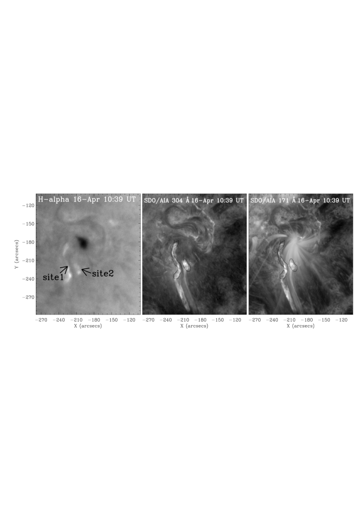
Figure 1.: Jets J₅ and J^′₅ from site 1 and site 2 respectively in the south of the main sunspot of AR 12035 on 16 April 2014 i.e. from left to right in H$\alpha$, observed in Nainital, India (ARIES), in 304 Å and in 171 Å observed with SDO/AIA. The contours of H$\alpha$ are over-plotted on to 304 Å and 171 Å. The jets look to be overlapping according to the scale resolution of the images. fig:hal

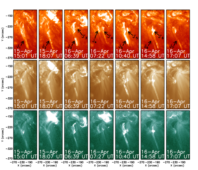
Figure 2.: Recurrent jets in the active region AR 12035 on 15 and 16 April 2014. Upper, middle and bottom panels are images of AIA filters at 304 Å, 193 Å, and 94 Å respectively. The arrows indicate the bright emission of the jets in two different locations mentioned as site 1 and site 2 in Figure fig:hal.fig:jet/morpho

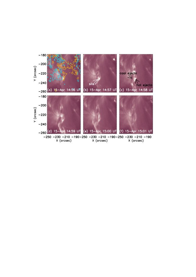
Figure 3.: Evolution of jet J₁ initiated in site 1 observed by AIA 211 Å. The contours on the first image are HMI longitudinal magnetic field with yellow and cyan colors for positive and negative polarities respectively. The contour levels are $\pm$100 Gauss. The site 1 is indicated by a white arrow. The cool and hot part of the ejected jet J₁ are indicated by black arrows.fig:jet1

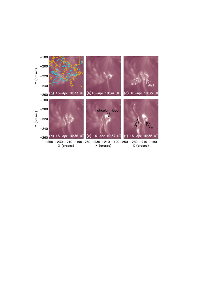
Figure 4.: Evolution of jets J₅ and J^′₅ from site 1 and site 2 (indicated by white arrows) observed by AIA 211 Å. The contours on the first image are HMI longitudinal magnetic field. Yellow and cyan colors are for positive and negative polarities respectively. The contour levels are $\pm$100 Gauss. The positions of jets J₅, J^′₅ and the circular ribbon are indicated by black arrows.fig:jet5

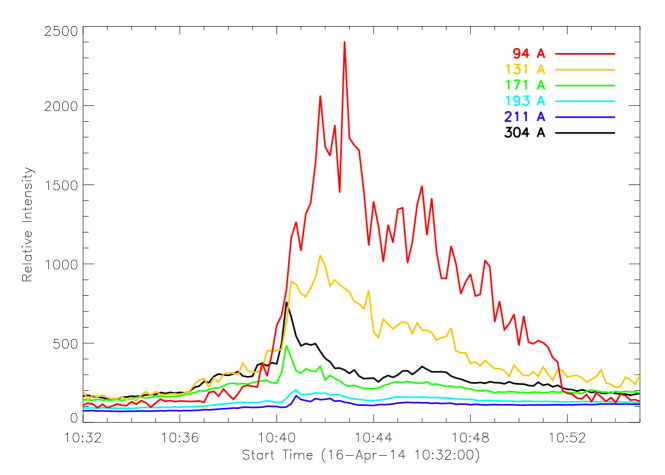
Figure 5.: Intensity profile of jet J₅ at base location. Different colors represent different SDO/AIA wavelengths. The peak of the cooler component is earlier (304 Å: longer wavelength) than the peak of the hotter component (94 Å: shorter wavelength).fig:inten

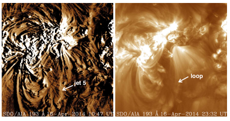
Figure 6.: Sigmoidal orientation of the loops in the active region in the AIA 193 Å  filter (right panel) and in the difference image (left panel). The jet J₅ follows the path of the loop.fig:loop

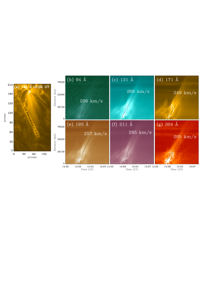
Figure 7.: Time-slice analysis of jet J₁ on 15 April 2014. Left: position of slit along the jet, right: velocity comparison at different wavelengths.fig:slice1

Figure 8.: An example of a height–time plot for Jet J₁ derived using the leading edge procedure.fig:leading˙edge

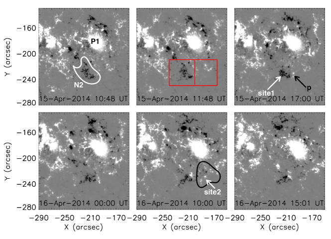
Figure 9.: Magnetic field evolution of NOAA active region 12035. The two jet locations (site 1 between N2 and p, site 2 at the edge of the supergranule indicated by the black contour) are indicated by white arrows. The red boxes in the left of the bottom panel show the site 1 (left) and site 2 (right) locations respectively and the field of view of Figures fig:mag1 and fig:mag2.fig:mag

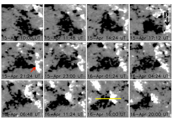
Figure 10.: Evolution of magnetic field at the site 1 location. The flux cancellation at site 1 between the negative polarity and the positive polarity (p) is shown by a red arrow. The horizontal yellow line indicates the location of the slit, where the time-distance evolution of flux is calculated (see Figure fig:mag_slice).fig:mag1

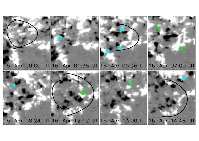
Figure 11.: Evolution of magnetic field at the site 2 location. The positive (negative) flux emergence is shown by green (cyan) arrows respectively. The roundish black curve indicate kind of supergranule cell.fig:mag2

Figure 12.: Magnetic field evolution along the slice shown in Figure 9 at site 1. Two vertical lines in the image indicate the time of jet activity.fig:mag˙slice

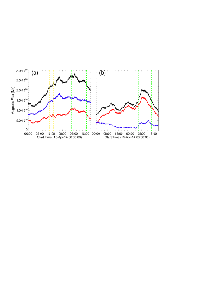
Figure 13.: Magnetic flux as a function of time calculated over the red box of Figure fig:mag for the site 1 (a) and site 2 (b) location. Black, red and blue curves are for total, positive and negative magnetic flux respectively. Jets on 15 April and 16 April occur in between the yellow and green dashed lines respectively.fig:mag˙evo

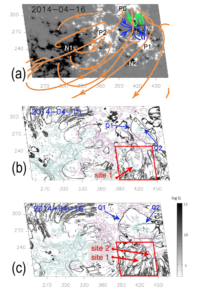
Figure 14.: Magnetic field (line of sight component) of AR 12035 for 16 April 2014. Panel (a) shows the two leading positive polarities P1 and P2 and the following negative polarity N1. The magnetic field is overlaid by magnetic field lines obtained from a potential extrapolation. Panels (b) and (c): Contours of the magnetic field overlaid by the footprints of the QSL at z=0.4 Mm above the photosphere, respectively for 15 April (b) and 16 April (c). Q1 and Q2 indicate the QSLs related to the flares, The magenta/cyan contours are drawn for levels of the magnetic field equal to $\pm 100,\pm 300,\pm 500,\pm 700,\pm 900$ Gauss. The red boxes indicate the region of the jets, site 1 on 15 April and both sites on 16 April. (adapted from Zuccarello et al. (2017)).fig:top

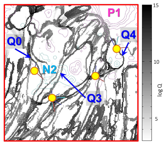
Figure 15.: Zoom of the jet region inside the red box of 16 April (see panel (c) in Figure fig:top). Q1 and Q2 indicate the QSLs related to the flares, Q3 and Q4 to the site 1 and site 2 of the jets respectively. The vertical color bar indicates the value of the squashing degree Q. The yellow circles indicate the positions of four null points. fig:null

Acknowledgments

The authors are thankful to the referee for the constructive comments and suggestions which improved the manuscript significantly. We acknowledge the SDO/AIA and HMI open data policy. RJ acknowledges the Department of Science and Technology (DST), Government of India for an INSPIRE fellowship. This work was initiated during the one month stay of RC at the Observatoire de Paris, LESIA, Meudon, France. RC also acknowledges the support from SERB–DST project no. SERB/F/7455/ 2017-17.

Disclosure of Potential Conflicts of Interest The authors declare that they have no conflicts of interest.

References

- Adams et al. (2014) Adams, M., Sterling, A.C., Moore, R.L., Gary, G.A.: 2014, A Small-scale Eruption Leading to a Blowout Macrospicule Jet in an On-disk Coronal Hole. ApJ 783, 11. DOI.
- Alexander and Fletcher (1999) Alexander, D., Fletcher, L.: 1999, High-resolution Observations of Plasma Jets in the Solar Corona. Sol. Phys. 190, 167. DOI.
- Alissandrakis (1981) Alissandrakis, C.E.: 1981, On the computation of constant alpha force-free magnetic field. A&A 100, 197.
- Archontis and Hood (2013) Archontis, V., Hood, A.W.: 2013, A Numerical Model of Standard to Blowout Jets. ApJ 769, L21. DOI.
- Asai, Ishii, and Kurokawa (2001) Asai, A., Ishii, T.T., Kurokawa, H.: 2001, Plasma Ejections from a Light Bridge in a Sunspot Umbra. ApJ 555, L65. DOI.
- Aulanier, Pariat, and Démoulin (2005) Aulanier, G., Pariat, E., Démoulin, P.: 2005, Current sheet formation in quasi-separatrix layers and hyperbolic flux tubes. A&A 444, 961. DOI.
- Berlicki et al. (2004) Berlicki, A., Schmieder, B., Vilmer, N., Aulanier, G., Del Zanna, G.: 2004, Evolution and magnetic topology of the M 1.0 flare of October 22, 2002. A&A 423, 1119. DOI.
- Chae et al. (1999) Chae, J., Qiu, J., Wang, H., Goode, P.R.: 1999, Extreme-Ultraviolet Jets and H Surges in Solar Microflares. ApJ 513, L75. DOI.
- Chandra et al. (2015) Chandra, R., Gupta, G.R., Mulay, S., Tripathi, D.: 2015, Sunspot waves and triggering of homologous active region jets. MNRAS 446, 3741. DOI.
- Chandra et al. (2017) Chandra, R., Mandrini, C.H., Schmieder, B., Joshi, B., Cristiani, G.D., Cremades, H., Pariat, E., Nuevo, F.A., Srivastava, A.K., Uddin, W.: 2017, Blowout jets and impulsive eruptive flares in a bald-patch topology. A&A 598, A41. DOI.
- Chen et al. (2015) Chen, J., Su, J., Yin, Z., Priya, T.G., Zhang, H., Liu, J., Xu, H., Yu, S.: 2015, Recurrent Solar Jets Induced by a Satellite Spot and Moving Magnetic Features. ApJ 815, 71. DOI.
- Cheung et al. (2015) Cheung, M.C.M., De Pontieu, B., Tarbell, T.D., Fu, Y., Tian, H., Testa, P., Reeves, K.K., Martínez-Sykora, J., Boerner, P., Wülser, J.P., Lemen, J., Title, A.M., Hurlburt, N., Kleint, L., Kankelborg, C., Jaeggli, S., Golub, L., McKillop, S., Saar, S., Carlsson, M., Hansteen, V.: 2015, Homologous Helical Jets: Observations By IRIS, SDO, and Hinode and Magnetic Modeling With Data-Driven Simulations. ApJ 801, 83. DOI.
- Dalmasse et al. (2012) Dalmasse, K., Pariat, E., Antiochos, S.K., DeVore, C.R.: 2012, Coronal jets in an inclined coronal magnetic field : a parametric 3D MHD study. In: Faurobert, M., Fang, C., Corbard, T. (eds.) EAS Publications Series, EAS Publications Series 55, 201. DOI.
- Dalmasse et al. (2015) Dalmasse, K., Chandra, R., Schmieder, B., Aulanier, G.: 2015, Can we explain atypical solar flares? A&A 574, A37. DOI.
- Demoulin (1998) Demoulin, P.: 1998, Magnetic Fields in Filaments (Review). In: Webb, D.F., Schmieder, B., Rust, D.M. (eds.) IAU Colloq. 167: New Perspectives on Solar Prominences, Astronomical Society of the Pacific Conference Series 150, 78.
- Demoulin et al. (1996) Demoulin, P., Henoux, J.C., Priest, E.R., Mandrini, C.H.: 1996, Quasi-Separatrix layers in solar flares. I. Method. A&A 308, 643.
- Dudík et al. (2012) Dudík, J., Aulanier, G., Schmieder, B., Zapiór, M., Heinzel, P.: 2012, Magnetic Topology of Bubbles in Quiescent Prominences. ApJ 761, 9. DOI.
- Fang, Fan, and McIntosh (2014) Fang, F., Fan, Y., McIntosh, S.W.: 2014, Rotating Solar Jets in Simulations of Flux Emergence with Thermal Conduction. ApJ 789, L19. DOI.
- Gu et al. (1994) Gu, X.M., Lin, J., Li, K.J., Xuan, J.Y., Luan, T., Li, Z.K.: 1994, Kinematic characteristics of the surge on March 19, 1989. A&A 282, 240.
- Guo et al. (2013a) Guo, Y., Démoulin, P., Schmieder, B., Ding, M.D., Vargas Domínguez, S., Liu, Y.: 2013a, Recurrent coronal jets induced by repetitively accumulated electric currents. A&A 555, A19. DOI.
- Guo et al. (2013b) Guo, Y., Démoulin, P., Schmieder, B., Ding, M.D., Vargas Domínguez, S., Liu, Y.: 2013b, Recurrent coronal jets induced by repetitively accumulated electric currents. A&A 555, A19. DOI.
- Hong et al. (2011) Hong, J., Jiang, Y., Zheng, R., Yang, J., Bi, Y., Yang, B.: 2011, A Micro Coronal Mass Ejection Associated Blowout Extreme-ultraviolet Jet. ApJ 738, L20. DOI.
- Innes, McIntosh, and Pietarila (2010) Innes, D.E., McIntosh, S.W., Pietarila, A.: 2010, STEREO quadrature observations of coronal dimming at the onset of mini-CMEs. A&A 517, L7. DOI.
- Innes et al. (2016) Innes, D.E., Bučík, R., Guo, L.-J., Nitta, N.: 2016, Observations of solar X-ray and EUV jets and their related phenomena. Astronomische Nachrichten 337, 1024. DOI.
- Jiang et al. (2007) Jiang, Y.C., Chen, H.D., Li, K.J., Shen, Y.D., Yang, L.H.: 2007, The H surges and EUV jets from magnetic flux emergences and cancellations. A&A 469, 331. DOI.
- Joshi et al. (2017) Joshi, N.C., Chandra, R., Guo, Y., Magara, T., Zhelyazkov, I., Moon, Y.-J., Uddin, W.: 2017, Investigation of recurrent EUV jets from highly dynamic magnetic field region. Ap&SS 362, 10. DOI.
- Kamio et al. (2007) Kamio, S., Hara, H., Watanabe, T., Matsuzaki, K., Shibata, K., Culhane, L., Warren, H.P.: 2007, Velocity Structure of Jets in a Coronal Hole. PASJ 59, S757. DOI.
- Kim, Kim, and Jang (2001) Kim, Y.-H., Kim, K.-S., Jang, M.: 2001, High-Speed x-ray Jets Associated with the 18 June 1999 Limb Flares. Sol. Phys. 203, 371. DOI.
- Lemen et al. (2012) Lemen, J.R., Title, A.M., Akin, D.J., Boerner, P.F., Chou, C., Drake, J.F., Duncan, D.W., Edwards, C.G., Friedlaender, F.M., Heyman, G.F., Hurlburt, N.E., Katz, N.L., Kushner, G.D., Levay, M., Lindgren, R.W., Mathur, D.P., McFeaters, E.L., Mitchell, S., Rehse, R.A., Schrijver, C.J., Springer, L.A., Stern, R.A., Tarbell, T.D., Wuelser, J.-P., Wolfson, C.J., Yanari, C., Bookbinder, J.A., Cheimets, P.N., Caldwell, D., Deluca, E.E., Gates, R., Golub, L., Park, S., Podgorski, W.A., Bush, R.I., Scherrer, P.H., Gummin, M.A., Smith, P., Auker, G., Jerram, P., Pool, P., Soufli, R., Windt, D.L., Beardsley, S., Clapp, M., Lang, J., Waltham, N.: 2012, The Atmospheric Imaging Assembly (AIA) on the Solar Dynamics Observatory (SDO). Sol. Phys. 275, 17. DOI.
- Liu et al. (2011) Liu, C., Deng, N., Liu, R., Ugarte-Urra, I., Wang, S., Wang, H.: 2011, A Standard-to-blowout Jet. ApJ 735, L18. DOI.
- Madjarska et al. (2013) Madjarska, M., Huang, Z., Subramanian, S., Doyle, G.: 2013, Jets from coronal holes - possible source of the slow solar wind. In: EGU General Assembly Conference Abstracts, EGU General Assembly Conference Abstracts 15, EGU2013.
- Mandrini et al. (1996) Mandrini, C.H., Démoulin, P., van Driel-Gesztelyi, L., Schmieder, B., Cauzzi, G., Hofmann, A.: 1996, 3D Magnetic Reconnection at an X-Ray Bright Point. Sol. Phys. 168, 115. DOI.
- Masson et al. (2009) Masson, S., Pariat, E., Aulanier, G., Schrijver, C.J.: 2009, The Nature of Flare Ribbons in Coronal Null-Point Topology. ApJ 700, 559. DOI.
- Moore et al. (2010) Moore, R.L., Cirtain, J.W., Sterling, A.C., Falconer, D.A.: 2010, Dichotomy of Solar Coronal Jets: Standard Jets and Blowout Jets. ApJ 720, 757. DOI.
- Moore et al. (2013) Moore, R.L., Sterling, A.C., Falconer, D.A., Robe, D.: 2013, The Cool Component and the Dichotomy, Lateral Expansion, and Axial Rotation of Solar X-Ray Jets. ApJ 769, 134. DOI.
- Moreno-Insertis and Galsgaard (2013) Moreno-Insertis, F., Galsgaard, K.: 2013, Plasma Jets and Eruptions in Solar Coronal Holes: A Three-dimensional Flux Emergence Experiment. ApJ 771, 20. DOI.
- Moreno-Insertis, Galsgaard, and Ugarte-Urra (2008) Moreno-Insertis, F., Galsgaard, K., Ugarte-Urra, I.: 2008, Jets in Coronal Holes: Hinode Observations and Three-dimensional Computer Modeling. ApJ 673, L211. DOI.
- Nisticò et al. (2009) Nisticò, G., Bothmer, V., Patsourakos, S., Zimbardo, G.: 2009, Characteristics of EUV Coronal Jets Observed with STEREO/SECCHI. Sol. Phys. 259, 87. DOI.
- Panesar, Sterling, and Moore (2017) Panesar, N.K., Sterling, A.C., Moore, R.L.: 2017, Magnetic Flux Cancelation as the Origin of Solar Quiet Region Pre-Jet Minifilaments. ArXiv e-prints. ADS.
- Pariat and Démoulin (2012) Pariat, E., Démoulin, P.: 2012, Estimation of the squashing degree within a three-dimensional domain. A&A 541, A78. DOI.
- Pariat, Antiochos, and DeVore (2009) Pariat, E., Antiochos, S.K., DeVore, C.R.: 2009, A Model for Solar Polar Jets. ApJ 691, 61. DOI.
- Pariat, Antiochos, and DeVore (2010) Pariat, E., Antiochos, S.K., DeVore, C.R.: 2010, Three-dimensional Modeling of Quasi-homologous Solar Jets. ApJ 714, 1762. DOI.
- Pariat et al. (2015) Pariat, E., Dalmasse, K., DeVore, C.R., Antiochos, S.K., Karpen, J.T.: 2015, Model for straight and helical solar jets. I. Parametric studies of the magnetic field geometry. A&A 573, A130. DOI.
- Pesnell, Thompson, and Chamberlin (2012) Pesnell, W.D., Thompson, B.J., Chamberlin, P.C.: 2012, The Solar Dynamics Observatory (SDO). Sol. Phys. 275, 3. DOI.
- Priest and Démoulin (1995) Priest, E.R., Démoulin, P.: 1995, Three-dimensional magnetic reconnection without null points. 1. Basic theory of magnetic flipping. J. Geophys. Res. 100, 23443. DOI.
- Priest and Forbes (1992) Priest, E.R., Forbes, T.G.: 1992, Magnetic flipping - Reconnection in three dimensions without null points. J. Geophys. Res. 97, 1521. DOI.
- Raouafi et al. (2016) Raouafi, N.E., Patsourakos, S., Pariat, E., Young, P.R., Sterling, A.C., Savcheva, A., Shimojo, M., Moreno-Insertis, F., DeVore, C.R., Archontis, V., Török, T., Mason, H., Curdt, W., Meyer, K., Dalmasse, K., Matsui, Y.: 2016, Solar Coronal Jets: Observations, Theory, and Modeling. Space Sci. Rev. 201, 1. DOI.
- Savcheva et al. (2009) Savcheva, A., Cirtain, J.W., DeLuca, E.E., Golub, L.: 2009, Does a Polar Coronal Hole’s Flux Emergence Follow a Hale-Like Law? ApJ 702, L32. DOI.
- Schmieder et al. (1983) Schmieder, B., Mein, P., Vial, J.-C., Tandberg-Hanssen, E.: 1983, Dynamics of a surge observed in the C IV and H alpha lines. A&A 127, 337.
- Schmieder et al. (2013) Schmieder, B., Guo, Y., Moreno-Insertis, F., Aulanier, G., Yelles Chaouche, L., Nishizuka, N., Harra, L.K., Thalmann, J.K., Vargas Dominguez, S., Liu, Y.: 2013, Twisting solar coronal jet launched at the boundary of an active region. A&A 559, A1. DOI.
- Schou et al. (2012) Schou, J., Scherrer, P.H., Bush, R.I., Wachter, R., Couvidat, S., Rabello-Soares, M.C., Bogart, R.S., Hoeksema, J.T., Liu, Y., Duvall, T.L., Akin, D.J., Allard, B.A., Miles, J.W., Rairden, R., Shine, R.A., Tarbell, T.D., Title, A.M., Wolfson, C.J., Elmore, D.F., Norton, A.A., Tomczyk, S.: 2012, Design and Ground Calibration of the Helioseismic and Magnetic Imager (HMI) Instrument on the Solar Dynamics Observatory (SDO). Sol. Phys. 275, 229. DOI.
- Shen et al. (2012) Shen, Y., Liu, Y., Su, J., Deng, Y.: 2012, On a Coronal Blowout Jet: The First Observation of a Simultaneously Produced Bubble-like CME and a Jet-like CME in a Solar Event. ApJ 745, 164. DOI.
- Shibata et al. (1992) Shibata, K., Ishido, Y., Acton, L.W., Strong, K.T., Hirayama, T., Uchida, Y., McAllister, A.H., Matsumoto, R., Tsuneta, S., Shimizu, T., Hara, H., Sakurai, T., Ichimoto, K., Nishino, Y., Ogawara, Y.: 1992, Observations of X-ray jets with the YOHKOH Soft X-ray Telescope. PASJ 44, L173.
- Shimojo and Shibata (2000) Shimojo, M., Shibata, K.: 2000, Physical Parameters of Solar X-Ray Jets. ApJ 542, 1100. DOI.
- Shimojo, Shibata, and Harvey (1998) Shimojo, M., Shibata, K., Harvey, K.L.: 1998, Magnetic Field Properties of Solar X-Ray Jets. Sol. Phys. 178, 379. DOI.
- Shimojo et al. (1996) Shimojo, M., Hashimoto, S., Shibata, K., Hirayama, T., Hudson, H.S., Acton, L.W.: 1996, Statistical Study of Solar X-Ray Jets Observed with the YOHKOH Soft X-Ray Telescope. PASJ 48, 123. DOI.
- Sterling and Moore (2016) Sterling, A.C., Moore, R.L.: 2016, A Microfilament-eruption Mechanism for Solar Spicules. ApJ 828, L9. DOI.
- Sterling et al. (2015) Sterling, A.C., Moore, R.L., Falconer, D.A., Adams, M.: 2015, Small-scale filament eruptions as the driver of X-ray jets in solar coronal holes. Nature 523, 437. DOI.
- Sterling et al. (2017) Sterling, A.C., Moore, R.L., Falconer, D.A., Panesar, N.K., Martinez, F.: 2017, Solar Active Region Coronal Jets II: Triggering and Evolution of Violent Jets. ArXiv e-prints. ADS.
- Titov, Hornig, and Démoulin (2002) Titov, V.S., Hornig, G., Démoulin, P.: 2002, Theory of magnetic connectivity in the solar corona. Journal of Geophysical Research (Space Physics) 107, 1164. DOI.
- Török et al. (2009) Török, T., Aulanier, G., Schmieder, B., Reeves, K.K., Golub, L.: 2009, Fan-Spine Topology Formation Through Two-Step Reconnection Driven by Twisted Flux Emergence. ApJ 704, 485. DOI.
- Uddin et al. (2012) Uddin, W., Schmieder, B., Chandra, R., Srivastava, A.K., Kumar, P., Bisht, S.: 2012, Observations of Multiple Surges Associated with Magnetic Activities in AR 10484 on 2003 October 25. ApJ 752, 70. DOI.
- Wang and Liu (2012) Wang, H., Liu, C.: 2012, Circular Ribbon Flares and Homologous Jets. ApJ 760, 101. DOI.
- Wyper, Antiochos, and DeVore (2017) Wyper, P.F., Antiochos, S.K., DeVore, C.R.: 2017, A universal model for solar eruptions. Nature 544, 452. DOI.
- Yokoyama and Shibata (1995) Yokoyama, T., Shibata, K.: 1995, Magnetic reconnection as the origin of X-ray jets and H surges on the Sun. Nature 375, 42. DOI.
- Yokoyama and Shibata (1996) Yokoyama, T., Shibata, K.: 1996, MHD Simulation of Solar Coronal X-ray Jets: Emerging Flux Reconnection Model. Astrophysical Letters and Communications 34, 133.
- Young and Muglach (2014) Young, P.R., Muglach, K.: 2014, Solar Dynamics Observatory and Hinode Observations of a Blowout Jet in a Coronal Hole. Sol. Phys. 289, 3313. DOI.
- Zhang et al. (2000) Zhang, J., Wang, J., Lee, C.-Y., Wang, H.: 2000, Macrospicules Observed with H Against the Quiet Solar Disk. DOI.
- Zhang et al. (2012) Zhang, Q.M., Chen, P.F., Guo, Y., Fang, C., Ding, M.D.: 2012, Two Types of Magnetic Reconnection in Coronal Bright Points and the Corresponding Magnetic Configuration. ApJ 746, 19. DOI.
- Zuccarello et al. (2017) Zuccarello, F.P., Chandra, R., Schmieder, B., Aulanier, G., Joshi, R.: 2017, The transition from eruptive to confined flares in the same active region. A&A 601, A26. DOI.