Anisotropy in the equation of state of strongly magnetized quark matter within the Nambu–Jona-Lasinio model Model

Abstract

In this article, we calculate the magnetization and other thermodynamical quantities for strongly magnetized quark matter within the Nambu-Jona-Lasinio model at zero temperature. We assume two scenarios, chemically equilibrated charge neutral matter present in the interior of compact stars and zero-strangeness isospin-symmetric matter created in nuclear experiments. We show that the magnetization oscillates with density but in a much more smooth form than what was previously shown in the literature. As a consequence, we do not see the unphysical behavior in the pressure in the direction perpendicular to the magnetic field that was previously found. Finally, we also analyze the effects of a vector interaction on our results.

I Introduction

Understanding dense and/or hot matter in the presence of strong magnetic fields is one of the most important challenges of nuclear physics today. At low chemical potentials, extremely high magnetic fields have been estimated to be breafly created in relativistic heavy-ion collisions Fukushima et al. (2008); Kharzeev and Warringa (2009); Kharzeev (2009); Skokov et al. (2009); Voronyuk et al. (2011), with strengths of up to $10^{19}$ and $10^{20}$ G expected to be generated during non-central heavy-ion collisions at the BNL Relativistic Heavy Ion Collider (RHIC) and at European Organization for Nuclear Research (CERN), respectively. In this regime, the role played by magnetic fields in quark deconfinement and chiral symmetry restoration can, to some extent, be extracted from lattice QCD data.

At low temperatures, high magnetic fields have been measured on the surface of neutron stars and extremely high magnetic fields have been inferred to exist in their interior. More specifically, measurements using anharmonic precession of star spin down have estimated surface magnetic fields to be of the order of $10^{15}$ G for the sources 1E 1048.1-5937 and 1E 2259+586 Melatos (1999) and data for slow phase modulations in star hard x-ray pulsations (interpreted as free precession) suggest internal magnetic fields to be on the magnitude of $10^{16}$ G for the source 4U 0142+61 Makishima et al. (2014). Together, these estimates have motivated a large amount of research on the issue of how magnetic fields modify the microscopic structure (represented in the equation of state) and the macroscopic structure (obtained from the solution of the Einstein-Maxwell’s equations) of neutron stars. Unfortunately, in this regime, there is no guidance from lattice QCD concerning the effect of magnetic fields on deconfined quark matter.

At high enough baryonic chemical potential/density a deconfinement transition to quark matter takes place and, when the temperature is low enough, other more complex phases such as color superconducting phases or inhomogeneous chiral condensates become energetically favorable. Much effort has been made to understand the physics of these phases in the presence of strong magnetic fields Ferrer and de la Incera (2013). The most favored phase of QCD at high densities is the color-flavor-looked (CFL) superconducting phase Alford et al. (1999) and, for a magnetic field strength of the order of the quark energy gap, a magnetic-CFL phase is preffered Ferrer and de La Incera (2007); de La Incera (2007); Ferrer et al. (2005, 2006a, 2006b). For field strengths comparable to the magnetic masses of charged gluons, the formation of a gluon-vortex state can take place Ferrer and de La Incera (2006); Ferrer and de la Incera (2007) and, as explained in Ferrer and de La Incera (2007), the vortex formation corresponds to a phase transition from a magnetic-CFL to a Paramagnetic-CFL phase. There are many other effects produced by a strong magnetic fields in combination with superconductivity Ferrer and de La Incera (2007); Noronha and Shovkovy (2007); Fukushima and Warringa (2008); Feng et al. (2011a, b, 2012), such as the BEC-BCS crossover Wang et al. (2011); Duarte et al. (2016); Fukushima et al. (2008); Duarte et al. (2017, 2016) and the modification of chiral inhomogeneous phases Frolov et al. (2010); Tatsumi et al. (2015); Ferrer et al. (2012); Carignano et al. (2015).

For simplicity, in this article we make use of the Nambu-Jona-Lasinio (NJL) model without pairing to describe zero strangeness isospin-symmetric matter (such as that created in nuclear experiments) and chemically equilibrated charge neutral matter (such as that present in the interiors of compact stars) to study how magnetic fields influence cold quark matter. We find that, unlike what was previously stated in the literature for this version of the model Menezes et al. (2015); Peres Menezes and Laércio Lopes (2016), strong magnetic fields do not generate unphysical behavior of thermodynamical quantities, such as the magnetization and pressure in the direction perpendicular to the magnetic field. In addition, we verify that our conclusions hold even when vector interactions (which allow us to reproduce astrophysical constraints) are added to the model.

II The Model

The description of matter in this work includes three-flavored quark matter and leptons (electrons and muons). While the leptons are described by a free Fermi gas under the influence of magnetic fields (which includes the quantization of Landau levels, see Ref. Strickland et al. (2012) and references therein for details), the description of strongly interacting quarks is much more complicated. The Lagrangian density for the SU(3) NJL model reads Nambu and Jona-Lasinio (1961a, b); Buballa (2005):

$${\pazocal L}_{f}={\pazocal L}_{Dir}+{\pazocal L}_{sym}+{\pazocal L}_{det}\ ,$$ (1)

where the different terms stand for the Dirac, symmetric (four-point interaction) and t’Hooft (six-point interaction) terms:

$${\pazocal L}_{Dir}={\bar{\psi}}_{f}\left[\gamma_{\mu}\left(i\partial^{\mu}-{\hat{q}}_{f}A^{\mu}\right)-{\hat{m}}_{c}\right]\psi_{f}\ ,$$ (2)

$${\pazocal L}_{sym}=G\sum_{a=0}^{8}\left[({\bar{\psi}}_{f}\lambda_{a}\psi_{f})^{2}+({\bar{\psi}}_{f}i\gamma_{5}\lambda_{a}\psi_{f})^{2}\right]\ ,$$ (3)

$${\pazocal L}_{det} = -K\big{\{}{\rm det}_{f}\left[{\bar{\psi}}_{f}(1+\gamma_{5})\psi_{f}\right]$$ (4)

$$+ {\rm det}_{f}\left[{\bar{\psi}}_{f}(1-\gamma_{5})\psi_{f}\right]\big{\}}\ ,$$

where $\psi_{f}=(u,d,s)^{T}$ represents the three-flavored quark field, while ${\hat{m}}_{c}={\rm diag}_{f}(m_{u},m_{d},m_{s})$ and ${\hat{q}}_{f}={\rm diag}(q_{u},q_{d},q_{s})$ are the quark mass and charge matrices. The interaction with the electromagnetic field appears in the Dirac term through the vector potential $A_{\mu}$. The coupling constants $G$ and $K$ are to be determined, $\lambda_{0}=\sqrt{2/3}I$ with $I$ being the unit matrix in the three flavor space, and $1<\lambda_{a}\leq 8$ denote the Gell-Mann matrices. For the leptons, we use the mass values $m_{e}=0.511$ MeV and $m_{\mu}=105.66$ MeV.

As the NJL model is non renormalizable, we apply a sharp ultraviolet cut-off $\Lambda$ in three-momentum space. The parameters of the model, $\Lambda$, $G$ and $K$, and the current quark masses, $m_{u}=m_{d}$ and $m_{s}$, are determined by fitting $f_{\pi}$, $m_{\pi}$, $m_{K}$, and $m_{\xi^{\prime}}$ to their empirical values. In this work, we adopt the parametrization proposed in Ref. Hatsuda and Kunihiro (1994) with $\Lambda=631.4$ MeV, $G=1.835/\Lambda^{2}$, $K=9.29/\Lambda^{5}$, $m_{u}=m_{d}=5.5$ MeV, and $m_{s}=135.7$ MeV.

The thermodynamical potential for the quark sector at zero temperature reads:

$$\Omega=-P={\pazocal E}-\sum_{f}{\mu}_{f}{\rho}_{f}\ ,$$ (5)

where $P$ (also referred to as $P_{\parallel}$) is the pressure in the direction of the magnetic field, ${\pazocal E}$ the energy density, $\mu_{f}$ the quark flavor chemical potential, and $\rho_{f}$ the quark flavor number density. A similar expression can be written for the leptonic sector. In the following results, normalization terms are implied in order to have $\Omega=0$ (and also $\Omega_{l}=0$ for the leptons) when the quark and leptonic chemical potentials are set to zero.

It is important to stress that in this work, as a result of the normalization described above, we do not account for the pure electromagnetic contribution in the Lagrangian density or in other thermodynamical quantities. The pure electromagnetic contribution is independent of any matter contribution, unless one is concerned with equilibrium configurations of macroscopic properties of stars and is solving Einstein s equations coupled to Maxwell’s equations, which is not the case in this work. For detailed analyses that compare pure magnetic field contributions with the ones from magnetized matter inside individual stars, see Refs. Chatterjee et al. (2015); Franzon et al. (2016).

II.1 Number density

In the mean field approximation, the quark number density for one quark flavor at zero temperature in the presence of an external magnetic field with strength $B$ in one direction is simply:

$$\rho_{f}=\sum_{\nu=0}^{\nu_{f,max}}\alpha_{\nu}\frac{|q_{f}|BN_{c}}{2\pi^{2}}p_{f}\ ,$$ (6)

where the sum over Landau levels $\nu$ goes until $\nu_{f,max}$ defined as the largest integer less than or equal to $({\mu_{f}^{2}-M_{f}^{2}})/({2|q_{f}|B})$. The degeneracy factor for each Landau level is $\alpha_{0}=1,\,\alpha_{k>0}=2$. $N_{c}$ is the number of colors and the energy dispersion is given by $\mu_{f}=\sqrt{p_{f}^{2}+s_{f}(\nu,B)^{2}}$, with $p_{f}$ being the Fermi momentum in the direction of the magnetic field and $s_{f}(\nu,B)=\sqrt{M_{f}^{2}+2|q_{f}|B\nu}$ the quark effective mass modified by the magnetic field.

II.2 Pressure

In the mean field approximation, the quark thermodynamical pressure can be written as:

$$P=\theta_{u}+\theta_{d}+\theta_{s}-2G(\phi_{u}^{2}+\phi_{d}^{2}+\phi_{s}^{2})+4K\phi_{u}\phi_{d}\phi_{s}\ ,$$

(7)

where the free terms containing the quark momenta and effective masses are:

$$\theta_{f}=-\frac{i}{2}{\rm tr}\int\frac{d^{4}p}{(2\pi)^{4}}\ln\left(-p^{2}+M_{f}^{2}\right)\ ,$$ (8)

while the scalar condensates are:

$$\phi_{f}=\langle{\bar{\psi}}_{f}\psi_{f}\rangle=-i\int\frac{d^{4}p}{(2\pi)^{4}}{\rm tr}\frac{1}{(\not\!p-M_{f}+i\epsilon)}\ ,$$ (9)

with traces taken over three colors and Dirac space (but not flavors). The quark effective masses can be obtained self consistently from:

$$M_{i}=m_{i}-4G\phi_{i}+2K\phi_{j}\phi_{k}\ ,$$ (10)

with $(i,j,k)$ being any permutation of flavors $(u,d,s)$.

We can rewrite Eq. (8) in terms of a vacuum, a medium and a magnetic contribution Menezes et al. (2009a, b):

$$\theta_{f}=\theta^{vac}_{f}+\theta^{med}_{f}+\theta^{mag}_{f}\ ,$$ (11)

which at zero temperature are given by:

$$\theta^{vac}_{f}=-\frac{N_{c}}{8\pi^{2}}\left\{M_{f}^{4}\ln\left[\frac{(\Lambda+\epsilon_{\Lambda})}{M_{f}}\right]-\epsilon_{\Lambda}\,\Lambda\left(\Lambda^{2}+\epsilon_{\Lambda}^{2}\right)\right\}\ ,$$

where $\epsilon_{\Lambda}=\sqrt{\Lambda^{2}+M_{f}^{2}}$,

$$\theta^{med}_{f} = \sum_{\nu=0}^{\nu_{f,max}}\alpha_{\nu}\frac{|q_{f}|BN_{c}}{4\pi^{2}}\Bigg{[}\mu_{f}\sqrt{\mu_{f}^{2}-s_{f}(\nu,B)^{2}}$$

$$- s_{f}(\nu,B)^{2}\ln\Bigg{(}\frac{\mu_{f}+\sqrt{\mu_{f}^{2}-s_{f}(\nu,B)^{2}}}{s_{f}(\nu,B)}\Bigg{)}\Bigg{]}\,,$$

and

$$\theta^{mag}_{f}=\frac{N_{c}(|q_{f}|B)^{2}}{2\pi^{2}}\left[\zeta^{\prime}(-1,x_{f})-\frac{1}{2}(x_{f}^{2}-x_{f})\ln x_{f}+\frac{x_{f}^{2}}{4}\right],$$

where we have $x_{f}=M_{f}^{2}/(2|q_{f}|B)$ and $\zeta^{\prime}(-1,x_{f})=d\zeta(z,x_{f})/dz|_{z=-1}$, with $\zeta(z,x_{f})$ being the Riemann-Hurwitz zeta function.

We can also rewrite Eq. (9) in terms of a vacuum, a medium and a magnetic contribution Menezes et al. (2009a, b), where the four-dimensional integrals gave rise to the sum over Landau levels in the medium contribution:

$$\phi_{f}=\phi_{f}^{vac}+\phi_{f}^{med}+\phi_{f}^{mag}\ ,$$ (15)

which at zero temperature are given by:

$$\phi_{f}^{vac} = -\frac{M_{f}N_{c}}{2\pi^{2}}\left[\Lambda\epsilon_{\Lambda}-{M_{f}^{2}}\ln\left(\frac{\Lambda+\epsilon_{\Lambda}}{{M_{f}}}\right)\right]\ ,$$ (16)

$$\phi_{f}^{med} = \sum_{\nu=0}^{\nu_{f,max}}\alpha_{\nu}\frac{M_{f}|q_{f}|BN_{c}}{2\pi^{2}}$$ (17)

$$\times \left[\ln\left(\frac{\mu_{f}+\sqrt{\mu_{f}^{2}-s_{f}(\nu,B)^{2}}}{s_{f}(\nu,B)}\right)\right]\ ,$$

$$\phi_{f}^{mag} = -\frac{M_{f}|q_{f}|BN_{c}}{2\pi^{2}}\Bigg{[}\ln\Gamma(x_{f})$$ (18)

$$- \frac{1}{2}\ln(2\pi)+x_{f}-\frac{1}{2}\left(2x_{f}-1\right)\ln(x_{f})\Bigg{]}\ .$$

In the direction perpendicular to the magnetic field, the pressure receives an extra contribution due to the quantization of the charged particles into the Landau levels Ferrer et al. (2010); Strickland et al. (2012):

$$P_{\perp}=P+{\cal M}B\ ,$$ (19)

where the magnetization ${\cal M}$ is going to be calculated in the following section.

For charge neutral $\beta$-equilibrated matter, an additional contribution to the pressure due to the leptons (electrons and muons) is added:

$$P_{l} = \theta^{med}_{l}=\sum_{\nu=0}^{\nu_{f,max}}\alpha_{\nu}\frac{B}{4\pi^{2}}\Bigg{[}\mu_{l}\sqrt{\mu_{l}^{2}-s_{l}(\nu,B)^{2}}$$ (20)

$$- s_{l}(\nu,B)^{2}\ln\Bigg{(}\frac{\mu_{l}+\sqrt{\mu_{l}^{2}-s_{l}(\nu,B)^{2}}}{s_{l}(\nu,B)}\Bigg{)}\Bigg{]}\ ,$$

where in the latter expression $s_{l}=\sqrt{m_{l}^{2}+2eB\nu}$. Note that only medium terms contribute to the pressure when a degenerate free gas of leptons is considered.

II.3 Vector interaction

One of the options for including a vector interaction in the NJL model gives the following extra term to be added to the Lagrangian Kitazawa et al. (2002); Fukushima (2008); Bratovic et al. (2013); Shao et al. (2013); Sasaki et al. (2013); Masuda et al. (2013):

$${\pazocal L}_{\rm{vec}}=-G_{V}({\bar{\psi}}\gamma^{\mu}\psi)^{2}\ ,$$ (21)

which was chosen because it reproduces a stiffer equation of state (EoS) and, consequently, more massive compacts stars Menezes et al. (2014). The constant $G_{V}$ was chosen to be equal to $G$ in order to maximize the effects of the vector interaction and allow one to test their effects in the presence of magnetic fields.

The pressure receives the following extra term due to the chosen vector interaction:

$$P_{\rm{vec}}=G_{V}(\rho_{u}+\rho_{d}+\rho_{s})^{2}\ ,$$ (22)

where $\rho=\rho_{u}+\rho_{d}+\rho_{s}=3\rho_{B}$ is the total quark density. As explained in Ref. Vogl and Weise (1991), in the mean field approximation, the role of the vector interaction is to introduce a shift in the quark chemical potential $\mu_{f}$ producing an effective quark chemical potential, $\tilde{\mu}_{f}=\mu_{f}-2G_{V}\rho$ to be taken into account in all thermodynamical quantities.

III Magnetization

In this section, we discuss the calculation of the magnetization emphasizing some fundamental points, which have been inappropriately considered in some recent publications Peres Menezes and Laércio Lopes (2016); Menezes et al. (2015). As explained in detail in Refs. Landau et al. (1984); Chaichian et al. (2000); Martinez et al. (2003); Ferrer et al. (2010); Strickland et al. (2012); D. Manreza Paret , the magnetization can be calculated simply by taking the partial derivative of the parallel pressure or, equivalently, minus the thermodynamical potential with respect to B:

$${\cal M}=\frac{\partial P}{\partial B}=-\frac{\partial\Omega}{\partial B}\ .$$ (23)

Next, we consider the magnetization calculation for the SU(3) NJL quark model including a vector interaction, since the extension to the simpler cases SU(2) and $G_{V}$=0 are trivial. As discussed in the previous section, the introduction of a vector interaction in the SU(3) NJL model within the mean field approximation is achieved by replacing the quark chemical potential $\mu_{f}$ by the corresponding quark effective chemical potential $\tilde{\mu}_{f}=\mu_{f}-2G_{V}\rho$. Thus, the grand potential for the quarks $\Omega(T,\{\mu_{f}\},B;\{\phi_{f}\},\rho)$ can be rewritten using Eq. (22):

$$\Omega = \sum_{f=u,d,s}\Omega_{f}+2G(\phi_{u}^{2}+\phi_{d}^{2}+\phi_{s}^{2})-4K\phi_{u}\phi_{d}\phi_{s}$$

$$+ G_{V}\rho^{2},$$

with each flavor contribution $\Omega_{f}(T,M_{f},\tilde{\mu}_{f},B)$ given by:

$$\Omega_{f}=-\left[\theta_{f}^{vac}+\theta_{f}^{med}\right.+\left.\theta_{f}^{mag}\right]\ .$$ (25)

The thermodynamically consistent solutions (discussed in Ref. Buballa (2005)) correspond to the stationary solutions of $\Omega$ as a function of $\phi_{f}$ and $\rho$ and are the key for the correct calculation of the magnetization, as shown in the following. It is easy to verify that one of the stationary solutions of the grand potential, Eq. (LABEL:omega1), is:

$$\frac{\partial\Omega}{\partial\phi_{f}}=0\ ,$$ (26)

where the condensate is given by:

$$\phi_{f}=\frac{\partial\Omega}{\partial m_{f}}=\frac{\partial\Omega}{\partial M_{f}}\ ,$$ (27)

with the corresponding gap equation, Eq. (10). Due to presence of the vector interaction, the grand potential becomes an explicit function of the total quark density and, once more, in order to assure thermodynamical consistency Vogl and Weise (1991); Buballa (2005), we have to impose a second stationary condition:

$$\frac{\partial\Omega}{\partial\rho}=0=\sum_{f=u,d,s}\frac{\partial\Omega}{\partial{\tilde{\mu}_{f}}}\frac{\partial{\tilde{\mu}_{f}}}{\partial\rho}+2G_{V}\rho\ ,$$ (28)

where we have used Eq. (LABEL:omega1) and:

$$\rho_{f}=-\frac{\partial\Omega}{\partial\mu_{f}}=-\frac{\partial\Omega}{\partial\tilde{\mu}_{f}}\ .$$ (29)

The constraint in the latter equation simply means that the total quark density has to satisfy the condition: $\rho=\rho_{u}+\rho_{d}+\rho_{s}$ in equilibrium. Both the gap equation and the latter constraint have to be simultaneously and self-consistently solved.

From Eq. (23), one may write:

$${\cal M}=-\left.\frac{\partial\Omega}{\partial B}\right|_{\{\phi_{f}\},\rho}-\frac{\partial\Omega}{\partial\phi_{f}}\frac{\partial\phi_{f}}{\partial B}-\frac{\partial\Omega}{\partial\rho}\frac{\partial\rho}{\partial B}\ ,$$ (30)

which can be simplified using Eq. (25) and the constraints given by Eqs. (26 and 29), yielding the following expression:

$${\cal M}=\sum_{f}\left[\frac{\partial\theta_{f}^{med}}{\partial B}+\frac{\partial\theta_{f}^{mag}}{\partial B}\right]\ .$$ (31)

This expression shows that only two terms contribute to the magnetization. Note that in Refs. Peres Menezes and Laércio Lopes (2016); Menezes et al. (2015) the derivatives of the $\phi^{\prime}s$ were incorrectly taken as being non-zero. Hence, a spurious increase of orders of magnitude was found in the magnetization in these references, which generated incorrect results for the perpendicular pressure leading the authors to erroneously conclude that strong anisotropy effects could exist for magnetic fields as small as 10¹⁷ Gauss.

The (non-zero) derivatives $\theta^{\prime}$ at $T=0$ are as in Ref. Menezes et al. (2015)

$$\theta^{\prime\,med}_{f} = \frac{\theta_{f}^{med}}{B}-\frac{N_{c}B|q_{f}|^{2}}{2\pi^{2}}\sum_{\nu=0}^{\nu_{max}}\alpha_{\nu}$$ (32)

$$\times \ln\left(\frac{\tilde{\mu}_{f}+\sqrt{\tilde{\mu}_{f}^{2}-s_{f}^{2}}}{s_{f}}\right)\nu\ ,$$

$$\theta^{\prime\,mag}_{f} = 2\frac{\theta^{mag}_{f}}{B}-\frac{N_{c}|q_{f}|M_{f}^{2}}{4\pi^{2}}\Bigg{[}\ln\Gamma(x_{f})-\frac{1}{2}\ln(2\pi)$$ (33)

$$+ x_{f}-(x_{f}-\frac{1}{2})\ln(x_{f})\Bigg{]}\ .$$

Note that, for the calculation within the SU(2) NJL model, we have only to take the summation over the flavors $u$ and $d$ in magnetization expression, Eq. (31).

For charge neutral $\beta$-equilibrated matter, the presence of the free gas of leptons gives an additional contribution to the magnetization, $\theta^{\prime}_{l}$,

$$\theta^{\prime\,med}_{l} = \frac{\theta_{l}^{med}}{B}-\frac{B}{2\pi^{2}}\sum_{\nu=0}^{\nu_{max}}\alpha_{\nu}\nu\ln\left(\frac{\mu_{l}+\sqrt{\mu_{l}^{2}-s_{l}^{2}}}{s_{l}}\right)\ ,$$

where only the medium term appears.

IV Results and discussion

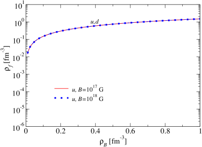
Figure 1: (Color online) Number density of each quark flavor for zero-strangeness isospin-symmetric matter. The different curves show density-independent magnetic field strengths of $10^{17}$ G and $10^{18}$ G. All curves overlap.

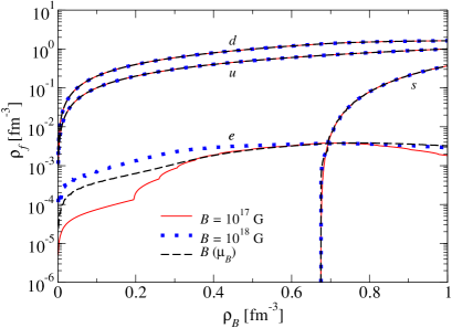
Figure 2: (Color online) Same as Fig. 1 but for charge neutral $\beta$-equilibrated neutron-star matter with electrons (the muons do not appear) also showing a realistic stellar chemical potential-dependent magnetic field from Ref. Dexheimer et al. (2016).

To exemplify the differences that appear when taking the derivatives of the $\phi^{\prime}s$ as (correctly) being zero, we remake some of the figures from Refs. Peres Menezes and Laércio Lopes (2016); Menezes et al. (2015) and point out the differences we find. In each figure we show different quantities as a function of baryon number density $\rho_{B}=\sum_{f}\rho_{f}/3$.

In different figures we show results for zero-strangeness isospin-symmetric matter and charge-neutral $\beta$-equilibrated neutron-star matter with leptons. In the first case, zero-strangeness is enforced at zero temperature simply by not including the strange quark. Isospin-symmetric matter is enforced by using the same chemical potential for up and down quarks $\mu_{u}=\mu_{d}=\mu_{B}/3$, where $\mu_{B}$ is the baryon chemical potential. In the second case, charge neutral matter is enforced by

$$\sum_{i}q_{i}\rho_{i}=0\ ,$$ (35)

where the index $i$ runs over quarks and leptons. $\beta$-equilibrium allows us to rewrite the fermion chemical potentials as a function of the chemical potentials related to the conserved quantities in the system, baryon and charge chemical potentials

$$\mu_{u}=\frac{1}{3}\mu_{B}+\frac{2}{3}\mu_{q}\ ,$$ (36)

$$\mu_{d}=\frac{1}{3}\mu_{B}-\frac{1}{3}\mu_{q}\ ,$$ (37)

$$\mu_{s}=\frac{1}{3}\mu_{B}-\frac{1}{3}\mu_{q}\ ,$$ (38)

$$\mu_{e}=\mu_{\mu}=-\mu_{q}\ ,$$ (39)

In different figures we show results for a density-independent magnetic field of strength $10^{17}$ G, a density-independent magnetic field of strength $10^{18}$ G, and a realistic (polar) stellar chemical potential-dependent field Dexheimer et al. (2016)

$$B^{*}(\mu_{B})=\frac{(a+b\mu_{B}+c\mu_{B}^{2})}{B_{c}^{2}}\ \mu,$$ (40)

with the baryon chemical potential $\mu_{B}$ given in MeV and the dipole magnetic moment $\mu$ in Am² in order to produce $B^{*}$ in units of the critical field of the electron $B_{c}=4.414\times 10^{13}$ G. The value of the coefficients for a star with baryon mass $M_{B}=1.6$ M_⊙(that gives a gravitational mass $\sim 1.4$ M_⊙) are $a=-1.02$ G²/(A m²), $b=1.58\times 10^{-3}$ G²/(A m² MeV), and $c=-4.85\times 10^{-7}$ G²/(A m² MeV²). We choose $\mu=2\times 10^{32}$ Am², which reproduces field strengths between $1.03\times 10^{17}$ and $5.31\times 10^{17}$ G in a $M_{B}=1.6$ M_⊙ star in the presence of a vector interaction.

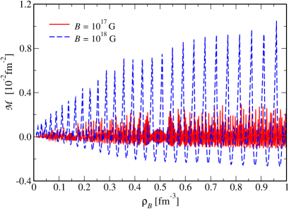
Figure 3: (Color online) Magnetization for zero-strangeness isospin-symmetric matter. The different curves show density-independent magnetic field strengths of $10^{17}$ G and $10^{18}$ G.

Figures 1 and 2 show the number density of each quark flavor (and leptons) for isospin-symmetric matter and neutron-star matter. In both cases, the effect of realistic magnetic fields (we did not include the case of a density-independent magnetic field with $10^{19}$ G) practically cannot be seen in the plots, in agreement with Refs. Peres Menezes and Laércio Lopes (2016); Menezes et al. (2015). As expected, in the zero-strangeness isospin-symmetric matter case, the amount of up and down quarks is the same for any baryon number density.

Figures 3 and 4 show the magnetization of the system for isospin-symmetric matter and neutron-star matter. In both cases, the effect of realistic magnetic fields produce magnetizations about three orders of magnitude lower in strength than in Refs. Peres Menezes and Laércio Lopes (2016); Menezes et al. (2015) and that oscillate (as in Ref. Huang et al. (2010)) but much less than in Refs. Peres Menezes and Laércio Lopes (2016); Menezes et al. (2015). The oscillations in the magnetization are unavoidable as Eqs. (32) and (33) have positive and negative terms. Note that even a free-Fermi gas produces oscillations in the magnetization with positive and negative values (for large enough magnetic field strength and density, see Refs. Strickland et al. (2012) and references therein for details). Note that the magnetization for the chemical-potential-dependent profile in Fig. 4 lies between the ones for fixed values $B=10^{17}$ and $B=10^{18}$ G.

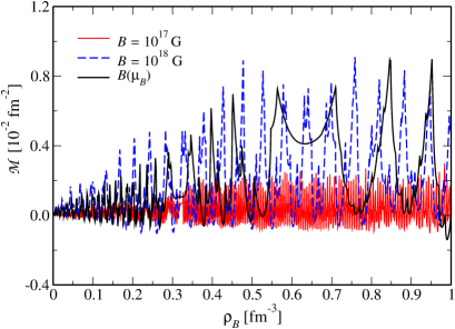
Figure 4: (Color online) Same as Fig. 3 but for charge neutral $\beta$ equilibrated neutron-star matter with electrons also showing a realistic stellar chemical potential-dependent magnetic field from Ref. Dexheimer et al. (2016).

Figures 5 and 6 show the parallel pressure of the system for isospin-symmetric matter and neutron-star matter. In both cases, the effect of realistic magnetic fields cannot be seen in the plots. This is in agreement with results from Refs. Peres Menezes and Laércio Lopes (2016); Menezes et al. (2015), except for the case with density-independent magnetic field with strength of $10^{19}$ G (not shown in our plots), in which case we would see the unphysical behavior of pressure going up and down with the increase of baryon number density or energy density, which means that the NJL model is unstable under those unphysical conditions. The reduction in the increase of pressure around $0.7$ fm^-3 in Fig. 6 is related to the appearance of the strange quarks in the system. The negative pressures at low densities in Figs. 5 and 6, on the other hand, indicate the presence of coexisting phases and associated phase transitions at those densities or, in other words, a crust is required for star stability Hanauske et al. (2001).

Figure 5: (Color online) Parallel and perpendicular pressures for zero-strangeness isospin-symmetric matter. The different curves show density-independent magnetic field strengths of $10^{17}$ G and $10^{18}$ G. All curves overlap.

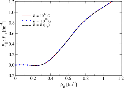
Figure 6: (Color online) Same as Fig. 5 but for charge neutral $\beta$ equilibrated neutron-star matter with electrons also showing a realistic stellar chemical potential-dependent magnetic field from Ref. Dexheimer et al. (2016). All curves overlap.

The perpendicular pressure of the system for isospin-symmetric matter and neutron-star matter is almost equal to the respective parallel pressures (Figs. 5 and 6), when using realistic magnetic fields (as already shown in Ref. Dexheimer et al. (2014) using the bag model). This is in disagreement with results from Refs. Peres Menezes and Laércio Lopes (2016); Menezes et al. (2015), in which case the perpendicular pressures are different for different magnetic field strengths, different from the respective parallel pressures and, most importantly, discontinuous.

Figure 7 shows that for magnetic field strengths slightly larger than of $10^{18}$ G, the pressure in the direction of the magnetic field (parallel) and perpendicular to it start to be different at any baryon number density. As already discussed in detail in Refs. Chatterjee et al. (2015); Franzon et al. (2016); Dexheimer et al. (2016), self-consistent general-relativity calculations assuming poloidal magnetic fields do not present solutions for stars that posses central magnetic fields beyond $1$ or $2$ times $10^{18}$ G. In this case, there would be no difference in using an EoS with magnetic field effects as input for those calculations (unlike what was stated in Refs. Peres Menezes and Laércio Lopes (2016); Menezes et al. (2015)). Note, however, that there are no consistent general relativity calculations of such kind using the NJL model with a vector interaction, in which case a much stiffer EoS might allow larger stellar central magnetic fields. This issue will be addressed in a future publication.

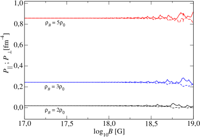
Figure 7: (Color online) Parallel (solid lines) and perpendicular (dotted lines) pressures for charge neutral $\beta$ equilibrated neutron-star matter with electrons as a function of magnetic field strength. The different curves show the pressures at different baryon number densities.

Figure 8: (Color online) Same as Fig. 2 but including a vector interaction.

Next, we present some results for charge neutral $\beta$-equilibrated matter including a vector interaction. These results are of special importance for magnetars and to our knowledge the magnetization study in this case has not yet been done in the literature. The change in the population due to the inclusion of a vector interaction is very small as can be seen in Fig. 8 (when compared with Fig. 2). Once more, the effect of all magnetic field strengths analyzed in this work practically does not modify the population. The changes in the magnetization with the inclusion of a vector interaction, on the other hand, are considerable, as can be seen in Fig. 9 (when compared with Fig. 4). The interaction leads the magnetization to oscillate more as a function of baryon number density, although it still has a low magnitude.

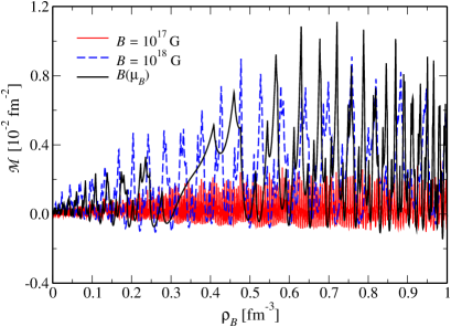
Figure 9: (Color online) Same as Fig. 4 but including a vector interaction.

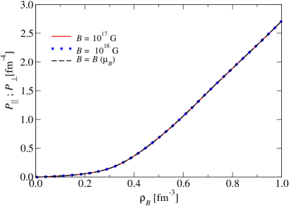
Figure 10: (Color online) Same as Fig. 6 but including a vector interaction.

As already discussed in the beginning of the section, when calculated correctly, the parallel and perpendicular pressures are almost equal when considering realistic magnetic fields. This does not change with the inclusion of a vector interaction as seen in Fig. 10. When compared with Fig. 6, it can be seen that the interaction makes the EoS of neutron star matter much stiffer, which is exactly why it is necessary to reproduce massive neutron stars. Note however that it has been shown that, for small chemical potentials, zero or a small vector interaction in quark matter is required in order to be in agreement with lattice QCD and perturbative QCD concerning baryon number susceptibilities Steinheimer and Schramm (2014); Bazavov et al. (2013); Haque et al. (2014). Nevertheless, whether or not those constraints are required at large chemical potentials is still an open question. Finally, we note that our results for the parallel pressures are in agreement with the results from Ref. Menezes et al. (2014), which includes magnetic field effects but does not calculate the magnetization.

V Conclusions and Outlook

In this work, we showed that the inclusion of magnetic fields in quark matter within the Nambu-Jona-Lasinio formalism does not generate the unphysical behavior previously found in Refs. Menezes et al. (2015); Peres Menezes and Laércio Lopes (2016) for the magnetization and pressure in the direction perpendicular to the magnetic field. We showed this for realistic magnetic fields, for zero-strangeness isospin-symmetric and neutron star (chemically equilibrated and charge neutral) matter, including or not a vector interaction. We found that up to magnetic field strengths of $10^{18}$ G, there is no change in population and there is no pressure anisotropy generated by the magnetic field (the pure electromagnetic contribution is not accounted for due to the normalization of the pressure). Although the magnetization oscillates with baryon number density, its magnitude is very small. A careful discussion on the calculation of the magnetization is presented and, in particular, the case where a vector interaction is present is analyzed, since, to our knowledge, this has not been done in the literature and is very important for the study of magnetars.

In a future publication, we are going to include our results with a strong vector interaction in a fully self-consistent general-relativity calculation to investigate if the interaction can increase the maximum stable stellar central magnetic field strength. A magnetic field strength of about $3\times 10^{18}$ G will already generate effects of the magnetic field in the equation of state.

References

References

- Fukushima et al. (2008) K. Fukushima, D. E. Kharzeev, and H. J. Warringa, Phys. Rev. D 78, 074033 (2008).
- Kharzeev and Warringa (2009) D. E. Kharzeev and H. J. Warringa, Phys. Rev. D 80, 034028 (2009).
- Kharzeev (2009) D. E. Kharzeev, Nuclear Physics A 830, 543c (2009), quark Matter 2009.
- Skokov et al. (2009) V. V. Skokov, A. Y. Illarionov, and V. D. Toneev, International Journal of Modern Physics A 24, 5925 (2009).
- Voronyuk et al. (2011) V. Voronyuk, V. D. Toneev, W. Cassing, E. L. Bratkovskaya, V. P. Konchakovski, and S. A. Voloshin, Phys. Rev. C 83, 054911 (2011).
- Melatos (1999) A. Melatos, Astrophys. J. 519, L77 (1999).
- Makishima et al. (2014) K. Makishima, T. Enoto, J. S. Hiraga, T. Nakano, K. Nakazawa, S. Sakurai, M. Sasano, and H. Murakami, Phys. Rev. Lett. 112, 171102 (2014).
- Ferrer and de la Incera (2013) E. J. Ferrer and V. de la Incera, in Lecture Notes in Physics, Berlin Springer Verlag, Lecture Notes in Physics, Berlin Springer Verlag, Vol. 871, edited by D. Kharzeev, K. Landsteiner, A. Schmitt, and H.-U. Yee (2013) p. 399, arXiv:1208.5179 [nucl-th] .
- Alford et al. (1999) M. Alford, K. Rajagopal, and F. Wilczek, Nuclear Physics B 537, 443 (1999), hep-ph/9804403 .
- Ferrer and de La Incera (2007) E. J. Ferrer and V. de La Incera, Phys. Rev. D 76, 045011 (2007), nucl-th/0703034 .
- de La Incera (2007) V. de La Incera, in VII LATIN American Symposium on Nuclear Physics and Applications, American Institute of Physics Conference Series, Vol. 947, edited by R. Alarcon, P. L. Cole, C. Djalali, and F. Umeres (2007) pp. 395–400, arXiv:0708.1619 [nucl-th] .
- Ferrer et al. (2005) E. J. Ferrer, V. de La Incera, and C. Manuel, Physical Review Letters 95, 152002 (2005), hep-ph/0503162 .
- Ferrer et al. (2006a) E. J. Ferrer, V. de la Incera, and C. Manuel, Nuclear Physics B 747, 88 (2006a), hep-ph/0603233 .
- Ferrer et al. (2006b) E. J. Ferrer, V. de la Incera, and C. Manuel, Journal of Physics A Mathematical General 39, 6349 (2006b), hep-ph/0511342 .
- Ferrer and de La Incera (2006) E. J. Ferrer and V. de La Incera, Physical Review Letters 97, 122301 (2006), hep-ph/0604136 .
- Ferrer and de la Incera (2007) E. J. Ferrer and V. de la Incera, Journal of Physics A Mathematical General 40, 6913 (2007), astro-ph/0611460 .
- Ferrer and de La Incera (2007) E. J. Ferrer and V. de La Incera, Phys. Rev. D 76, 114012 (2007), arXiv:0705.2403 [hep-ph] .
- Noronha and Shovkovy (2007) J. L. Noronha and I. A. Shovkovy, Phys. Rev. D 76, 105030 (2007), arXiv:0708.0307 [hep-ph] .
- Fukushima and Warringa (2008) K. Fukushima and H. J. Warringa, Phys. Rev. Lett. 100, 032007 (2008).
- Feng et al. (2011a) B. Feng, E. J. Ferrer, and V. de la Incera, Nuclear Physics B 853, 213 (2011a), arXiv:1105.2498 [nucl-th] .
- Feng et al. (2011b) B. Feng, E. J. Ferrer, and V. de la Incera, Physics Letters B 706, 232 (2011b), arXiv:1109.3100 [nucl-th] .
- Feng et al. (2012) B. Feng, E. J. Ferrer, and V. de la Incera, Phys. Rev. D 85, 103529 (2012), arXiv:1203.1630 [hep-th] .
- Wang et al. (2011) J.-C. Wang, V. de La Incera, E. J. Ferrer, and Q. Wang, Phys. Rev. D 84, 065014 (2011), arXiv:1012.3204 [nucl-th] .
- Duarte et al. (2016) D. C. Duarte, P. G. Allen, R. L. S. Farias, P. H. A. Manso, R. O. Ramos, and N. N. Scoccola, Phys. Rev. D 93, 025017 (2016), arXiv:1510.02756 [hep-ph] .
- Duarte et al. (2017) D. C. Duarte, P. G. Allen, R. L. S. Farias, P. H. A. Manso, and N. N. Scoccola, Proceedings, 7th International Workshop on Astronomy and Relativistic Astrophysics (IWARA 2016): Gramado, Brazil, October 9-13, 2016, Int. J. Mod. Phys. Conf. Ser. 45, 1760066 (2017).
- Duarte et al. (2016) D. C. Duarte, R. L. S. Farias, P. H. A. Manso, and R. O. Ramos, Proceedings, 13th International Workshop on Hadron Physics: Angra dos Reis, Rio de Janeiro, Brazil, March 22-27, 2015, J. Phys. Conf. Ser. 706, 052010 (2016).
- Frolov et al. (2010) I. E. Frolov, V. C. Zhukovsky, and K. G. Klimenko, Phys. Rev. D 82, 076002 (2010), arXiv:1007.2984 [hep-ph] .
- Tatsumi et al. (2015) T. Tatsumi, K. Nishiyama, and S. Karasawa, Physics Letters B 743, 66 (2015), arXiv:1405.2155 [hep-ph] .
- Ferrer et al. (2012) E. J. Ferrer, V. de la Incera, and A. Sanchez, Three days on quarkyonic islands. Proceedings, HIC for FAIR Workshop and 28th Max Born Symposium, Wroclaw, Poland, May 19-21, 2011, Acta Phys. Polon. Supp. 5, 679 (2012), arXiv:1205.4492 [nucl-th] .
- Carignano et al. (2015) S. Carignano, E. J. Ferrer, V. de la Incera, and L. Paulucci, Phys. Rev. D 92, 105018 (2015), arXiv:1505.05094 [nucl-th] .
- Menezes et al. (2015) D. P. Menezes, M. B. Pinto, and C. Providência, Phys. Rev. C91, 065205 (2015).
- Peres Menezes and Laércio Lopes (2016) D. Peres Menezes and L. Laércio Lopes, Eur. Phys. J. A52, 17 (2016), [Eur. Phys. J.A52,17(2016)], arXiv:1505.06714 [nucl-th] .
- Strickland et al. (2012) M. Strickland, V. Dexheimer, and D. P. Menezes, Phys. Rev. D86, 125032 (2012), arXiv:1209.3276 [nucl-th] .
- Nambu and Jona-Lasinio (1961a) Y. Nambu and G. Jona-Lasinio, Phys. Rev. 124, 246 (1961a).
- Nambu and Jona-Lasinio (1961b) Y. Nambu and G. Jona-Lasinio, Phys. Rev. 122, 345 (1961b).
- Buballa (2005) M. Buballa, Phys. Rept. 407, 205 (2005), arXiv:hep-ph/0402234 [hep-ph] .
- Hatsuda and Kunihiro (1994) T. Hatsuda and T. Kunihiro, Phys. Rept. 247, 221 (1994), arXiv:hep-ph/9401310 [hep-ph] .
- Chatterjee et al. (2015) D. Chatterjee, T. Elghozi, J. Novak, and M. Oertel, Mon. Not. Roy. Astron. Soc. 447, 3785 (2015), arXiv:1410.6332 [astro-ph.HE] .
- Franzon et al. (2016) B. Franzon, V. Dexheimer, and S. Schramm, Mon. Not. Roy. Astron. Soc. 456, 2937 (2016), arXiv:1508.04431 [astro-ph.HE] .
- Menezes et al. (2009a) D. P. Menezes, M. Benghi Pinto, S. S. Avancini, A. Perez Martinez, and C. Providência, Phys. Rev. C79, 035807 (2009a), arXiv:0811.3361 [nucl-th] .
- Menezes et al. (2009b) D. P. Menezes, M. Benghi Pinto, S. S. Avancini, and C. Providência, Phys. Rev. C80, 065805 (2009b), arXiv:0907.2607 [nucl-th] .
- Ferrer et al. (2010) E. J. Ferrer, V. de la Incera, J. P. Keith, I. Portillo, and P. L. Springsteen, Phys. Rev. C 82, 065802 (2010).
- Kitazawa et al. (2002) M. Kitazawa, T. Koide, T. Kunihiro, and Y. Nemoto, Prog. Theor. Phys. 108, 929 (2002), arXiv:hep-ph/0207255 [hep-ph] .
- Fukushima (2008) K. Fukushima, Phys. Rev. D77, 114028 (2008), [Erratum: Phys. Rev.D78,039902(2008)], arXiv:0803.3318 [hep-ph] .
- Bratovic et al. (2013) N. M. Bratovic, T. Hatsuda, and W. Weise, Phys. Lett. B719, 131 (2013), arXiv:1204.3788 [hep-ph] .
- Shao et al. (2013) G. Y. Shao, M. Colonna, M. Di Toro, Y. X. Liu, and B. Liu, Phys. Rev. D87, 096012 (2013), arXiv:1305.1176 [nucl-th] .
- Sasaki et al. (2013) T. Sasaki, N. Yasutake, M. Kohno, H. Kouno, and M. Yahiro, (2013), arXiv:1307.0681 [hep-ph] .
- Masuda et al. (2013) K. Masuda, T. Hatsuda, and T. Takatsuka, PTEP 2013, 073D01 (2013), arXiv:1212.6803 [nucl-th] .
- Menezes et al. (2014) D. P. Menezes, M. B. Pinto, L. B. Castro, P. Costa, and C. Providência, Phys. Rev. C89, 055207 (2014), arXiv:1403.2502 [nucl-th] .
- Vogl and Weise (1991) U. Vogl and W. Weise, Prog. Part. Nucl. Phys. 27, 195 (1991).
- Landau et al. (1984) L. D. Landau, E. M. Lifshitz, and L. P. Pitaevskii, Electrodynamics of Continuous Media. Vol. 8 (ButterworthÐHeinemann, 1984).
- Chaichian et al. (2000) M. Chaichian, S. S. Masood, C. Montonen, A. Pérez Martínez, and H. Pérez Rojas, Phys. Rev. Lett. 84, 5261 (2000).
- Martinez et al. (2003) A. P. Martinez, H. P. Rojas, and H. J. Mosquera Cuesta, Eur. Phys. J. C29, 111 (2003), arXiv:astro-ph/0303213 [astro-ph] .
- (54) A. P. M. D. Manreza Paret, J. E. Horvath, arXiv:1407.2280 [astro-ph.HE] .
- Dexheimer et al. (2016) V. Dexheimer, B. Franzon, R. O. Gomes, R. L. S. Farias, S. S. Avancini, and S. Schramm, (2016), arXiv:1612.05795 [astro-ph.HE] .
- Huang et al. (2010) X.-G. Huang, M. Huang, D. H. Rischke, and A. Sedrakian, Phys. Rev. D81, 045015 (2010), arXiv:0910.3633 [astro-ph.HE] .
- Hanauske et al. (2001) M. Hanauske, L. M. Satarov, I. N. Mishustin, H. Stoecker, and W. Greiner, Phys. Rev. D64, 043005 (2001), arXiv:astro-ph/0101267 [astro-ph] .
- Dexheimer et al. (2014) V. Dexheimer, D. P. Menezes, and M. Strickland, J. Phys. G41, 015203 (2014), arXiv:1210.4526 [nucl-th] .
- Steinheimer and Schramm (2014) J. Steinheimer and S. Schramm, Phys. Lett. B736, 241 (2014), arXiv:1401.4051 [nucl-th] .
- Bazavov et al. (2013) A. Bazavov, H. T. Ding, P. Hegde, F. Karsch, C. Miao, S. Mukherjee, P. Petreczky, C. Schmidt, and A. Velytsky, Phys. Rev. D88, 094021 (2013), arXiv:1309.2317 [hep-lat] .
- Haque et al. (2014) N. Haque, J. O. Andersen, M. G. Mustafa, M. Strickland, and N. Su, Phys. Rev. D89, 061701 (2014), arXiv:1309.3968 [hep-ph] .