Semantic Preserving Embeddings for Generalized Graphs

1 Introduction

In this work we present a new approach to the treatment of property graphs using neural encoding techniques derived from machine learning. Specifically, we will deal with the problem of embedding property graphs in vector spaces.

Throughout this paper we will use the term embedding as an operation that allows to consider a mathematical structure, $X$, inside another structure $Y$, through a function, $f:X\rightarrow Y$. We are interested on embeddings capable of capturing, within the characteristics of a vector space (distance, linearity, clustering, etc.), the interesting features of the graph.

For example, it would be interesting to get embeddings that, when projecting the nodes of the graph into points of a vector space, keep edges with the same type of the graph into the same vectors. In this way, we can interpret that the semantic associated to the relation has been captured by the embedding. Another option is to check if the embedding verifies clustering properties with respect to the types of nodes, types of edges, properties, or some of the metrics that can be measured on the graph.

Subsequently, we will use these good embedding features to try to obtain prediction / classification / discovery tools on the original graph.

This paper is structured as follows: we will start by giving some preliminary definitions necessary for the presentation of our proposal and a brief introduction to the use of artificial neural networks as encoding machines. After this review, we will present our embedding proposal based on neural encoders, and we will verify if the topological and semantic characteristics of the original graph have been maintained in the new representation. After evaluating the properties of the new representation, it will be used to carry out machine learning and discovery tasks on real databases. Finally, we will present some conclusions and future work proposals that have arisen during the implementation of this work.

2 Previous Definitions

2.1 Generalized Graphs

The definition of Generalized Graph that we present below unifies different graph definitions that can be found in the literature, and allows to have a general framework to support the data structures necessary for our proposal. More information about generalized graphs can be found in [1].

Definition 1.

A Generalized Graph is a tuple $G=(V,E,\mu)$ where:

• $V$ and $E$ are sets, called, respectively, set of nodes and set of edges of $G$.

• $\mu$ is a relation (usually functional, but not necessarily) that associates each node or edge in the graph with a set of properties, that is, $\mu:(V\cup E)\times R\rightarrow S$, where $R$ represents the set of possible keys for available properties, and $S$ the set of possible values associated.

Usually, for each $\alpha\in R$ and $x\in V\cup E$, we write $\alpha(x)=\mu(x,\alpha)$.

In addition, we require the existence of a special key for the edges of the graph, called incidences and denoted by $\gamma$, which associates to each edge of the graph a tuple, ordered or not, of vertices of the graph.

Although the definition that we have presented here is more general than those from related literature, we will also call them Property Graphs, since they are a natural extension of this type of graphs.

It should be noted that in generalized graphs, unlike traditional definitions, the elements in $E$ are symbols representing the edges, and not pairs of elements of $V$ and $\gamma$ is the function that associates to each edge the set of vertices that it relates. Generalized graphs represent a simple and powerful generalization for most existing graph definitions and allow for working with broader concepts, such as hypergraphs, in a natural way.

2.2 Encoding Neural Networks

Prediction-related tasks represent the most common application of feedforward neural networks. In this section we present this kind of networks from a diferent perspective, using them in a way that will be (and has been) of fundamental importance for the new results that have been obtained with them.

A neural encoder is a neural network used for learning codings for datasets. Note that when a feedforward neural network has hidden layers, all the communication that occurs between input and output layer passes through each of the hidden layers. Thus, if we are trying to approximate a function by means of a feedforward network, after setting the parameters of the network we can interpret that a given hidden layer keeps the information required from the input data for the calculation of the function. Therefore, always from the point of view of the function that calculates the network, we can say that the section of the network from the input layer to the hidden layer encodes the input data, and the weights (and bias) of this section of the network define the encoding function between both spaces [13]. Similarly, we can understand that the part of the original network that goes from this hidden layer to the output layer defines a decoding function (see Figure 1).

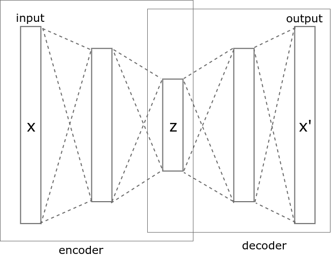
Figure 1: Neural Encoder

If we leave aside the posterior layers (including the original output layer) and the associated parameters, we obtain a new neural network that produces as output a representation of the input space into a specific dimension vector space (the number of neurons in the hidden layer). We must remember that this representation is achieved as partial application of a complete feedforward network that approximates a prefixed function and, consequently, this coding is relative to this function (and, of course, to the approximation process).

An autoencoder is a specific neural encoder where the function to learn is the identity function and, consequently, the input and output layers have the same number of neurons. As with normal encoders, when the network reaches an acceptable state (it is able to show an output similar enough to the input), the activations in the units of the hidden layers represent the encoding of the original data presented in the input layer [2].

If the number of units in the hidden layer differs from the number of units in the input layer (and output) we are also making a dimensional change when performing the encoding. In fact, this is one of the available methods to perform dimensionality changes by maintaining the structural characteristics (eg, proximity or similarity relations) of the training sets.

In this work we use neural encoders as a tool to perform generalized graph embeddings into vector spaces. Neural networks trained on adequate functions are used in order to verify to what extent semantic structures of the graph are conserved in the new vector space representation.

3 Related Works

The application of neural encoders to texts has provided very interesting results. In 2013, T. Mikolov et al. [16] presented two new architectures, under the generic name of word2vec, to learn vector representations of words trying to minimize computational complexity while maintaining the grammatical properties present in the texts from which they are extracted: Continuous bag-of-words (CBOW) and Skip-gram. In this task the context of a word in a text is defined as the set of words that appear in adjacent positions to it. The two architectures presented in [16] consist of feedforward artificial neural networks with $3$ layers: an input layer, a hidden layer (encoding layer) and an output layer, but they differ in the objective function they try to approximate. On the one hand, neural encoders with CBOW architecture receive the context of a given word as input and try to predict the word in its output. By contrast, encoders with Skip-gram architecture receive the word as input and try to predict the context associated with it. The main objective of the work of Mikolov et al. is to reduce the complexity in the neural model allowing the system to learn from a large volume of textual data. Until the arrival of word2vec, none of the available architectures had been able to train with more than a few million words. Through the relationship established between vocabulary words and their contexts, the model captures different types of similarity [17], both functional and structural, and provides an embedding of words in vector space that reflects these similarities.

In recent years different methods that try to learn vector representations of entities and relations in knowledge databases have been developed [11, 4, 21]. All of them represent the entities as elements of a given vector space and the relationships as a combination of the representations of the entities that participate in it.

In [4], embeddings of multi-relational data in vector space trying to verify some additional properties are proposed. Specifically, they look for a projection of nodes and types of edges, $\pi$, in vector space with two goals:

1. To minimize the distance $d(\pi(s)+\pi(l),\pi(t))$ from each existing (observed) relation $(s\xrightarrow{l}t)$ in the dataset, where $s$ represents the source element of the relation, $l$ represents the relationship type, and $t$ represents the target element of the relation.

2. To maximize the distances $d(\pi(s^{\prime})+\pi(l),\pi(t))$, $d(\pi(s)+\pi(l^{\prime}),\pi(t))$ and $d(\pi(s)+\pi(l),\pi(t^{\prime}))$, where $s^{\prime}$ and $t^{\prime}$ represent graph nodes, and $l^{\prime}$ represents a type of relationship of the graph, for which the relations $s^{\prime}\xrightarrow{l}t$, $s\xrightarrow{l}t^{\prime}$ and $s\xrightarrow{l^{\prime}}t$ do not exist (unobserved relationships) in the graph.

To improve the efficiency of the algorithm, the authors randomly sample the original graph for both existing and non-existing relationships. In [11], and in order to achieve better results in the projection, the authors follow a similar procedure but making use of a Siamese Neural Network . In [23] some of these techniques are grouped together on the same general theoretical framework making it possible to compare the complexity of the models and the obtained results.

Despite the relationship between these works and our approach, the requirement to maximize unobserved relationships (essential for the results they obtain) works against one of the objectives we pursue, since we do not assume that the original graph has complete information and, in our context, random unobserved links creation is not a good idea. Moreover, the prediction of this kind of links is one of the task that we pursue.

In other cases, works that perform vector embedding of entities and relations in knowledge databases learns representation of the entities using the prediction of unobserved links (Link Prediction) as objective function, conditioning the embedding with a supervised learning. In our case, the encoding is only conditioned by the similarity of the contexts in which the entities are immersed, opening the possibility of using these representations to a wider range of tasks.

DeepWalk [18] is a recent methodology that uses neural encoders to obtain vector representations nodes in uni-relational graphs using a very similar idea to word2vec. In this work the uni-relational graph is linearized using truncated random paths, interpreting the obtained paths as sentences. Subsequently, and completely equivalent to word2vec, they use these paths to train a neural encoder with Skip-gram architecture and to obtain an embedding of the nodes of the uni-relational graph in a vector space. This method does not allow to work with large uni-relational graphs efficiently, nor with multi-relational graphs.

LINE [22] is able to learn $d$-dimensional representations of uni-relational graph nodes through two phases: first it learns $d/2$ dimensions generating random paths in Breath-First Search mode, then it learns the remaining $d/2$ dimensions by sampling the nodes that are strictly at distance 2 from the embedding node.

Node2vec [12] groups and extends the ideas presented in DeepWalk and LINE. Specifically, the authors develop a flexible algorithm that, through two hyperparameters, allows to modify the generation of random paths that explore the environment of the nodes and that become their contexts. Based on two standard search strategies, Breath-First Sampling (BFS) and Depth-First Sampling (DFS), the two hyperparameters allow to control whether the random paths tend to a BFS or DFS strategy. In particular, they assert that a sampling guided by a BFS strategy results in embeddings reflecting structural equivalence between entities and that a sampling driven by a DFS strategy results in a embedding in which the homophilia is reflected. In this sense, DeepWalk is a specific case of this model. Node2vec have been evaluated in Multi-Label Classification and Link Prediction tasks.

In recent years, some works that use convolutional neural networks (CNN) to create vector representations of the nodes of uni-relational graphs have been published. In [15], the objective is to learn a function that encodes nodes by constructing descriptions of them. Outputs that represent the complete graph can also be obtained by applying some pooling operation [9]. In [8], the authors work with the convolution operator in the Fourier field, and generalize the convolutional networks to go from their original definition in low-dimensional regular euclidean spaces (where we work with images, videos or audio) to be able to work with high-dimensional irregular domains (multi-relational graphs obtained from social networks or biological phenomena). In [20] an extension of the Graph Convolutional Network [15] called the Relational Graph Convolutional Network is presented, which allows learning through the convolution and pooling operations typical of convolutional networks on multi-relational graphs.

In [19], the Graph Neural Network Model is defined, which converts the data graph into a recurrent neural network, and each node in a multi-layer feedforward network. The combination of these structures allows supervised learning where many of the weights of the network are shared, reducing the learning cost.

In Heterogeneous Network Embedding [7], a framework to perform network embeddings connecting data of different types in low-dimensional spaces is presented. As the model perform unsupervised learning, the new representation is adequate for any prediction task since it has not be conditioned. Using these representations, in [14] they face the task of automatically assign tags to nodes of different types in a heterogeneous network that has no types in the edges. The algorithm is designed to learn dependencies between node tags and to infer them exploiting the properties of the global graph and the characteristics of the neighbours of nodes. They impose two objectives: (1) grouping nodes of the same type that are connected (with less intensity as longer is the path connecting them), and (2) grouping nodes of different types if they share contexts. When working with property graphs, properties are represented as nodes.

As we have shown, there are numerous methodologies that allows to perform vector embedding of graphs, some of them are limited to working with uni-relational graphs, others are conditioned through the generation of unobserved relationships or do not capture the global semantic characteristics of a property graph. Our proposal, which we detail below, aims to obtain embeddings that are not affected by these limitations.

4 Generalized Graph Embeddings

The selected architecture for our neural encoder is CBOW because, despite its simplicity and the low computational training cost, it obtains good results capturing both syntactical and semantic relations [16].

In a first approximation, and in order to evaluate to what extent the semantic structure given by the edges is maintained, we will make a projection on the vector space using only the set of nodes, $V$. In this way, following the analogy offered by the word2vec algorithm, our vocabulary will be the set of nodes of the graph and their associated properties values, $S$.

A context, $C$, associated to a node $n\in V$ is obtained by randomly selecting a number of neighbouring nodes to $n$ and their properties (selecting elements from $\mathcal{N}(n)\cup\mu(n,\cdot)$), regardless of the edges that connects them and of the type of property. The number of selected nodes/properties determines the selection window size.

Following a similar methodology to those from the previous section, we will generate a training set consisting of pairs $(n,C)$, where $n\in V$ and $C$ is one of its associated contexts. The neural encoder is trained using this training set and then the activations of the hidden layer of the neural network are used as vector representation of each node. Algorithm 1, GG2Vec, shows the followed procedure.

1:  $training\_set=\{\}$

2:  for each $0<i\leq N$ do

3:     $n$ = randomly selected element from $V_{G}$

4:     $C=\{\}$

5:     for each $0<i\leq ws$ do

6:        $e$ = randomly selected element from $\mathcal{N}(n)\cup\mu_{G}(n)$

7:        $C=C\cup\{e\}$

8:     end for

9:     $training\_set=training\_set\cup\{(v,C)\}$

10:  end for

11:  Train a $CBOW$-like architecture with $D$ neurons in hidden layer using $training\_set$

12:  return  The resulting encoding for each element in $V$

Algorithm 1 GG2Vec($G$,$N$,$ws$,$D$)

We will use these vector representations trying to solve some classification and discovery tasks in the original graph. The results of these tasks will provide a measure of reliability on the achieved embedding (Fig. 2).

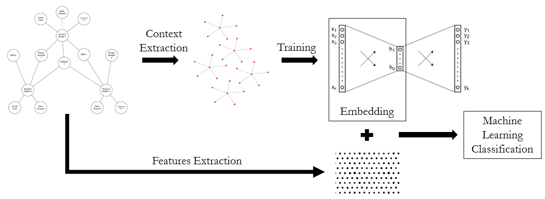
Figure 2: Proposed Methodology Representation

In the embedding procedure the free parameters of the model, which will have to be adjusted in the various experiments to analyze its effectiveness and viability, are:

• $D$, number of neurons in the hidden layer, determines the dimension of the vector space where we will embed the elements of the graph.

• $N$, size of the training set, number of pairs $(n,C)$ used to train the encoder.

• $ws$, selection window size, number of neighbours and properties considered to construct the contexts of nodes in $V$.

In what follows, we will note by $\pi:V\to\mathbb{R}^{D}$ the embedding obtained from the trained neural encoder.

Despite generalized graphs allow hypergraph definition, next we present the embedding procedure for binary links because the databases that we use in the experiments represent binary relational data. After obtaining an embedding of the nodes of the graph, an embedding of the edges in the same vector space is induced (which will also be noted by $\pi$) in the following way:

Definition 2.

If $G=(V,E,\tau,\mu)$ is a binary Generalized Graph, and $\pi:V\to\mathbb{R}^{D}$ is a node embedding, we extend $\pi:E\to\mathbb{R}^{D}$ by:

$$e\in E,\ s\overset{e}{\rightarrow}t\mbox{, then }\pi(e)=\overrightarrow{\pi(s)\pi(t)}$$

Since the usual operations in vector spaces are widely used in current computation units (processors and GPUs), this new representation can be used to analyze, repair and extract information from multi-relational datasets efficiently. Some tasks that can improve with this type of embeddings are:

• Clusters formed by nodes/edges in the new vector space can be used to induce missing properties in the elements of the graph (making use of distance, linearity or clustering relationships, for example).

• Vector representations of the elements of a graph can help to obtain measures of similarity between them.

• Analysis of vectors associated with the different families of relations (those sharing a common type, or verifying similar properties, for example) can help to detect missing relationships in the original dataset that in the new representation become evident. If the position of two nodes complies with the representative vector of some type of relation, maybe those nodes should be connected by an edge with this type although that relation does not appear in the graph.

• The representation of graph paths in the new space can help to develop more efficient ways to perform multi-relational queries.

5 Empirical Evaluation

Let us perform some empirical evaluations of our method with two differentiated objectives:

1. To analyse that the obtained vectorial representations maintain semantic characteristics of the original graphs.

2. To perform classification and discovery tasks making use of the resulting embeddings.

We will say that an embedding respects the semantics of a property graph if, from the new representation, it is possible to obtain the types associated with nodes and edges despite them have not being present during the embedding process. The type of each node or edge will be determined by a key $\tau\in R$. In order to perform this verification, the several embeddings we will calculate will not receive information about types of nodes or edges in the original the graph (formally, they will not receive information about $\tau$). Hence, contexts associated with nodes of the graph, which are used to create the training set, are generated by randomly selecting a number ($ws$) of neighbouring nodes and values of their different properties in $\mu$ excluding $\tau$.

5.1 Implementation details and experiments

Python has been chosen as programming language to perform the experimental evaluation . CBOW architecture implementation of Gensim toolkit (version 0.12.4) has been used. In addition, Neo4j has been used as a persistence system.

Each embedding experiment, has been repeated 10 times, obtaining a standard deviation smaller than $2\%$ in type prediction experiments. In the case of tasks related to Entity Retrieval these deviation is bounded by $8\%$ and in the case of obtaining the target nodes of a typed path is bounded by $8.9\%$.

Machine learning models used to learn from the new data representations are$k$-NN, Random Forest and Neural Networks. For the general classification tests, and unless otherwise is indicated, $k$-NN with $k=3$ has been used as base comparison model.

5.2 Datasets

The experiments were carried out in 3 different graph databases, two of them widely known by the data analysis community: WordNet and TheMovieDB. The third is a data set about the ecuadorian intangible cultural heritage.

Datasets have been partially manipulated to reduce their size and complexity. Below we give some details about each of these graphs in order to contextualize the characteristics that we will find in the results.

WordNet® [10] is a database of english nouns, verbs, adjectives and adverbs. It is one of the most important resources in the area of computational linguistics, and has been built as a combination of dictionary and thesaurus, designed to be intuitive. Each element in the database represents a list of synonymous words (which they call synset), and the relationships that are established between the elements occur both at lexical and semantic level. In this work we have used a section of the 3.0 version, considering only entities and relations that are shown in Figure 3 (in a similar way to [11]), obtaining a graph with 97,593 nodes and 240,485 relations, with the distribution of types shown in Figure 4.

Figure 3: WordNet Schema

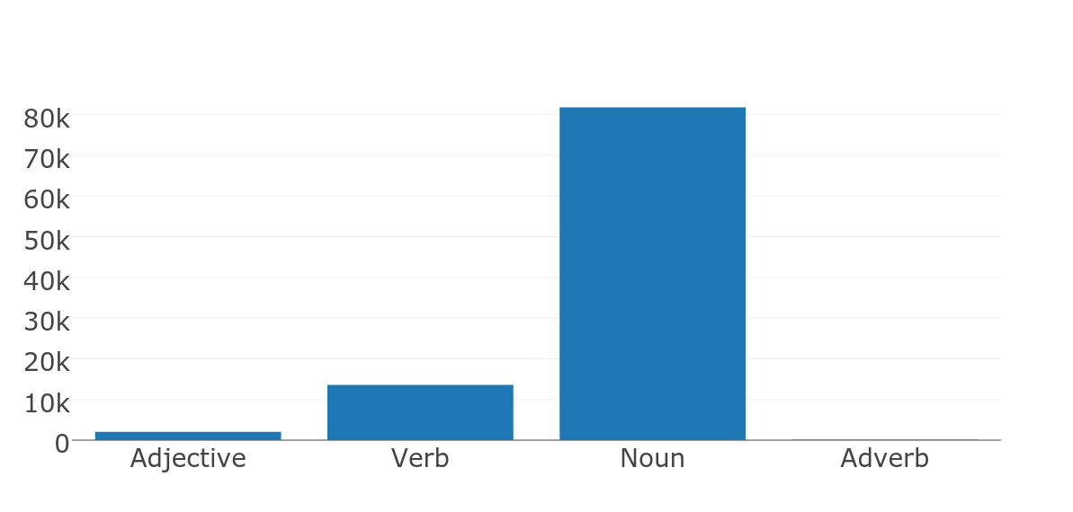
(a) Node types distribution

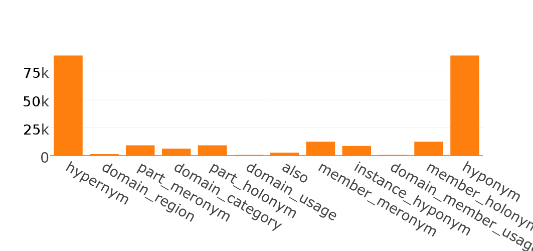
(b) Edge types distribution

Figure 4: Nodes and edges distribution in WordNet

TheMovieDB (TMDb) is a dataset with information about actors, movies and television content. For our experiments we have considered all the TMDb entities that are connected by relations belonging to the types acts_in, directed, genre and studio, obtaining a graph with 66,020 nodes and 125,624 relations. Figure 5 shows a graphical representation of the data schema, and Figure 6 shows the distribution by types of nodes and edges of this dataset.

Figure 5: TMDb schema

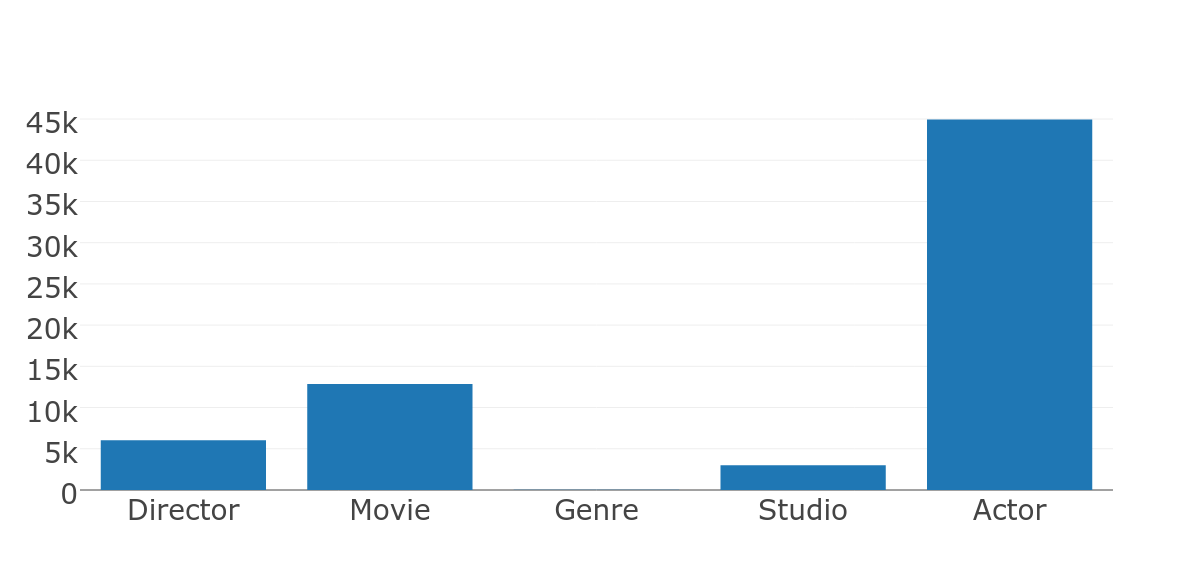
(a) Node types distribution

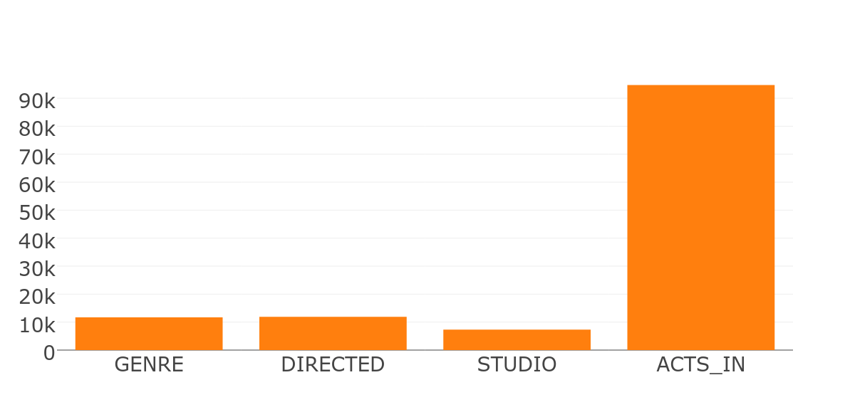
(b) Edge types distribution

Figure 6: Nodes and edges distribution in TMDb.

It should be noted that Actor and Director types are overlapping, specifically in our dataset there are 44,097 nodes associated only to Actor type, 5,191 nodes associated only to Director type, and 846 nodes with both types simultaneously (multi-type nodes).

Ecuadorian Intangible Cultural Heritage (EICH Database of Ecuador) corresponds to a section of the National Institute of Ecuadorian Cultural Heritage database which contains 38,990 nodes and 55,358 relations distributed through 11 types of nodes and 10 types of edges, with information about the intangible cultural heritage of Ecuador. This database is the most heterogeneous of the three analysed, presenting more typology in both nodes and edges, and also its elements have more properties than the other two considered datasets. Figures 7 and 8 show the schema and distribution of nodes and edges in this graph, respectively.

Figure 7: EICH schema

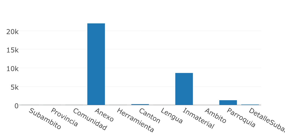
(a) Node types distribution

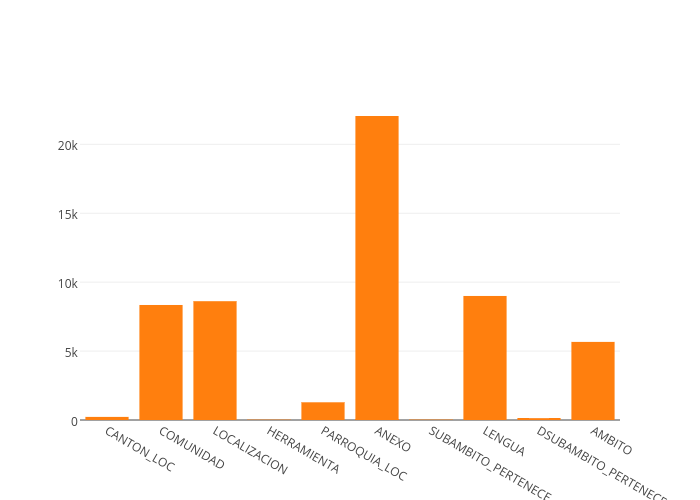
(b) Edge types distribution

Figure 8: Nodes and edges distribution in EICH

If we define the semantic richness of a node as the sum of the number of relations it participates in and the number of properties it possesses, we can construct the histogram of semantic richness for each dataset (Fig. 9). In the case of WordNet, the average semantic richness is 5.56, in the case of TMDb it is 3.21, and in the case of EICH it is 7.86. The different behaviour of this distribution in the studied cases may be help to understand the results.

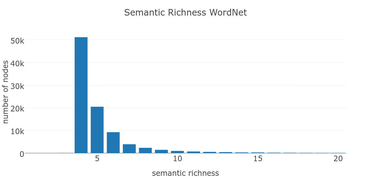
(a) WordNet

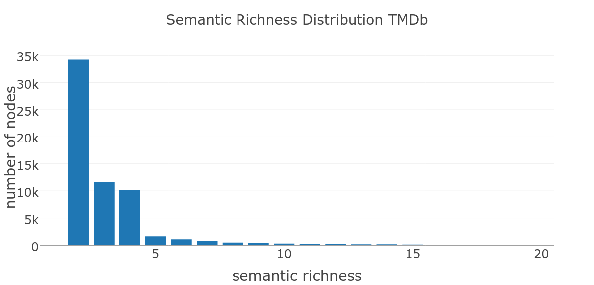
(b) TMDb

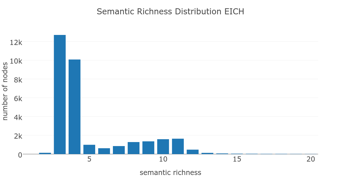
(c) EICH

Figure 9: Semantic Richness (less than 20)

5.3 Node Types Prediction

Our first experiment aims to predict $\tau$ function. In a similar way, we could try to predict any property of $\mu$, always being careful that it is not used during training.

A first intuition about how the achieved embeddings maintain the semantic structures can be obtained by analysing how the various types are distributed in the vector space.

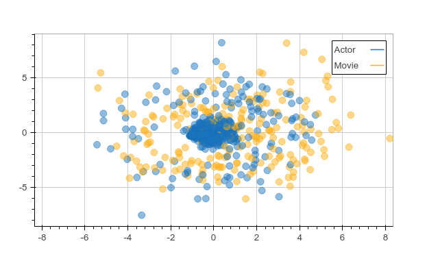
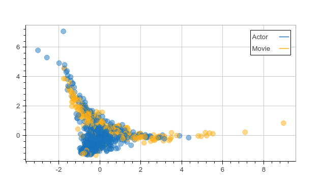
Figure 10: 2D representations of Movie and Actor nodes in TMDb

Figure 10 shows two projections of a section of TMDb graph embedding. The representation on the left shows a random selection of Movie and Actor nodes using a embedding in a space of 200 dimensions (which has been projected later on a two-dimensional space using Multi-Dimensional Scaling [5]), while the representation on the right shows the same section of the graph making use of an embedding on a 2 dimension space. Although the dimensionality reduction considered is clearly excessive (but necessary to visualize the data in these pages), both representations show that the TMDb nodes are not randomly distributed with respect to the types, which shows that, the embedding maintains information relative to the type of nodes, and we consider that the embedding process captures the semantic associated to node types.

In addition to the freedom of choice over the parameters involved in the encoding, we find some additional degrees of freedom when deciding which machine learning methiod will be used to learn from the vector representation of the nodes in a graph. As a first approximation, an exhaustive study of the free parameters of the model has been made using the classification method $k$-NN. The reason for choosing this model focuses on two fundamental aspects: it depends only on its own parameter (the value of $k$, which is known to work relatively well for $k=3$) and, in spite of its simplicity, provides robust results that serve as a comparative basis for other more sophisticated classification models.

Table 1: Embedding optimal parameters

	$N$	$D$	Selection Window Size	Prediction
TMDb	400.000	150	3	$\simeq 72\%$
WordNet	1.000.000	50	8	$\simeq 96\%$
EICH	300.000	20	2	$\simeq 83\%$

Table 1 shows optimal values of free parameters of the embedding using $k$-NN as a later learning model (with $k=3$). Figure 11 shows the results of this analysis for the three considered graphs, where prediction rates above 70 % are obtained for all of them.

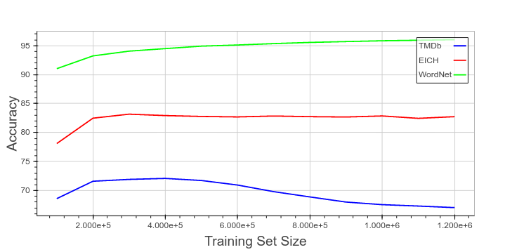
(a) Depending on the the training set size

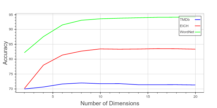
(b) Depending on the number of dimensions

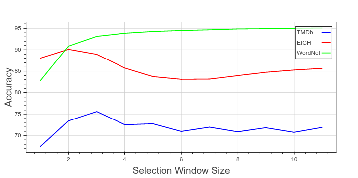
(c) Depending on the selection window size

Figure 11: Immersion analysis (node type prediction)

In all cases, the optimal training set size to perform the automatic prediction of node types is proportional to the number of nodes in the graph. Both EICH and TMDb (for WordNet we do not know the optimal value, because it is increasing in the analysed range) show a reduction in the prediction rate from the optimum value, this can be due to an overfitting related to the existence of nodes of different types with the same label.

Regarding the vector space dimension, no big changes can be observed when we increase $D$ above 10-15, a relatively low dimension, but it is almost imperceptible. We can interpret that around 10-15 dimensions are enough to capture the complexity of the analysed graphs.

The study of the influence of the selection window size ($ws$) shows that small values of this parameter are required to obtain good results in the prediction of node types. It is important to note that the best prediction is not achieved in any case with $ws=1$, since this would mean that the system does not need to receive node-context pairs as elements of the training set but would suffice to show instances of the relations present in each node.

5.3.1 Using other prediction models

Once the parameters of the embedding shown in Table 1 are set, we proceed to compare the predictive capacity with some other classification methods on the same task. Specifically, we will compare the results of $k$-NN with those obtained through Random Forest and Feedforward Neural Networks.

Figure 12 shows obtained results. (a) Shows the variation of the results provided by $k$-NN depending on $k$. In (b), results obtained varying the number of trees using Random Forest as a later machine learning are shown. Finally, in (c) the results of the neural network are shown when the number of neurons in the hidden layer is modified.

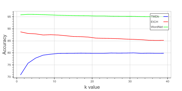
(a) k-Nearest Neighbor

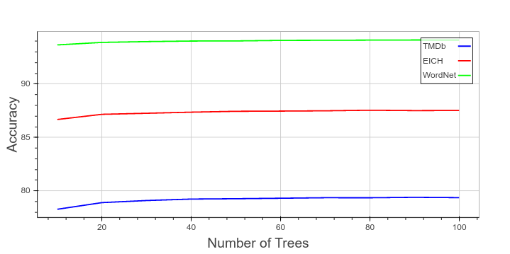
(b) Random Forest

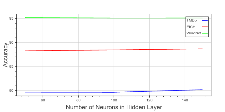
(c) Feddforward Neural Network

Figure 12: Analysis of the node types classification using different Machine Learning methods

We also present averaged confusion matrices after performing 10 experiments using the optimal parameters indicated above and $k$-NN: WordNet (Table 2), TMDb (Table 3), and EICH (Table 8). These matrices capture the semantic similarities between node types. In EICH, for example, Canton, Parroquia and Provincia show overlapping behaviour because they all represent highly correlated geospatial information. In TMDb something similar occurs, ACTOR and DIRECTOR nodes appear related because, as we mentioned, there are numerous nodes in this database having both types simultaneously.

Table 2: Confusion Matrix: Node types prediction (WordNet)

	adjective	verb	noun	adverb
adjective	90.01%	1.75%	8.2%	0.05%
verb	0.44%	88.36%	11.19%	0.0%
noun	0.2%	1.56%	98.23%	0.01%
adverb	10.16%	1.63%	29.27%	58.94%

Table 3: Confusion Matrix: Node types prediction (TMDb)

	Director	Movie	Genre	Studio	Actor
Director	11.45%	9.54%	0.02%	1.48%	77.51%
Movie	6.51%	65.8%	0.02%	0.29%	27.37%
Genre	9.66%	33.79%	2.07%	3.45%	51.03%
Studio	9.66%	8.49%	0.01%	1.23%	80.61%
Actor	5.77%	7.87%	0.0%	0.7%	85.66%

5.4 Edge Types Prediction

The second experiment aims to determine the goodness of the embedding in edge types prediction task.

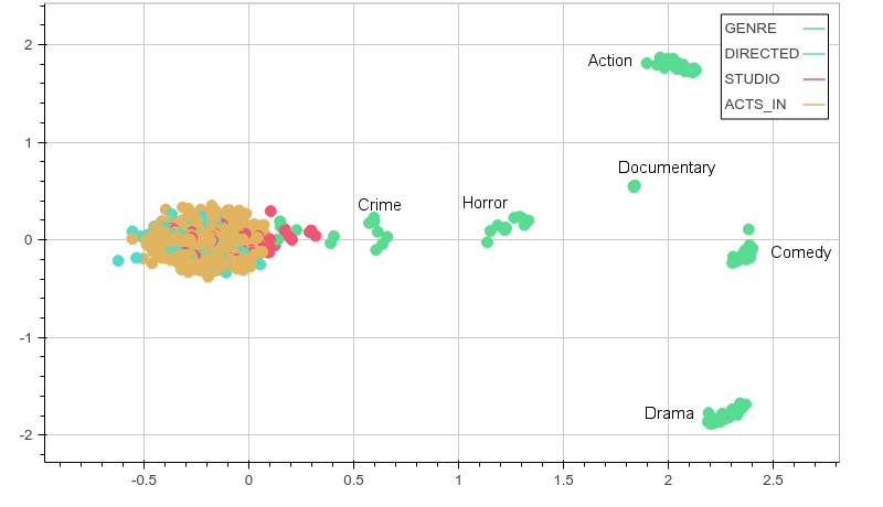
Figure 13: 2D Representation of edges in TMDb

Figure 13 shows a two-dimensional projection from a randomly selected set of edges of the TMDb dataset. It can be observed that Genre edges do not form a single cluster, but a collection of peripheral ones that corresponding to values Action, Comedy, Drama, Documentary, Horror and Crime, showing a different semantic behaviour respect other edge types. This might indicate that Genre may not form a semantically unique edge type, and that its behaviour reflects some heterogeneity in design decisions when constructing the original database model. It is here where this type of analysis shows unique characteristics that can make it suitable to be used as an additional normalizer to databases covering also semantic and not only structural information.

In Figure 14, results of edge type prediction using $k$-NN method are shown. Taking into account that the percentage of correctness is above 80 % in all the studied datasets (even over 95 % in some of them), we can conclude that our embedding methodology maintains the semantic properties of the edges.

In general, we can observe that the training set size necessary to obtain good results when predicting edge types is superior to that required to make a good prediction of the node types for the three analysed graphs. In addition, although WordNet is the dataset with best results when predicting node types, in the case of edge types the best results are obtained for EICH.

As in the previous case, embeddings require a relatively low dimension, $D\simeq 15$.

The behaviour of edge types prediction tasks according to $ws$ shows values higher than those required for nodes. In any case, it is important to note that, again, the best prediction is not achieved in any case with $ws=1$.

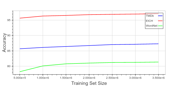
(a) Depending on the training set size

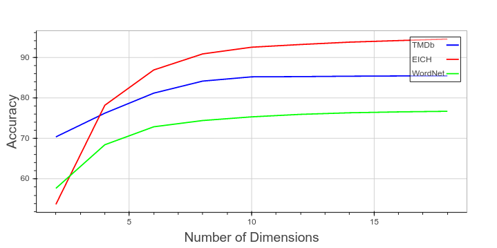
(b) Depending on the number of dimensions

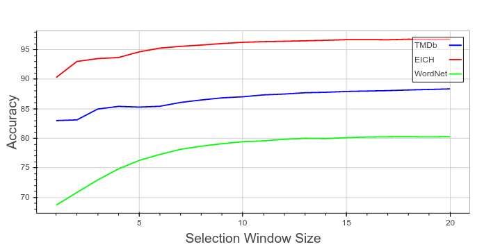
(c) Depending on the selection window size

Figure 14: Embedding Analysis (link types prediction)

5.4.1 Using other prediction models

Following the same methodology as for node types, Figure 15 shows results obtained by the three same automatic classification methods in the edge types prediction case. These classification tasks were performed with embeddings using the parameters presented in Table 1.

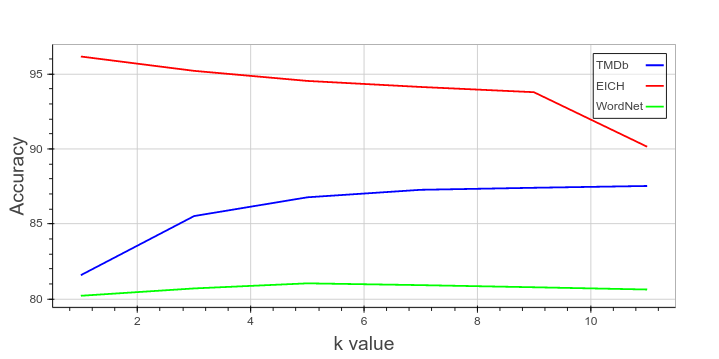
(a) k-Nearest Neighbor

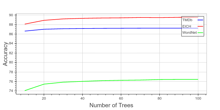
(b) Random Forest

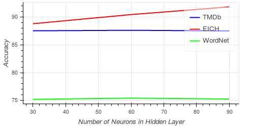
(c) Feedforward Neural Network

Figure 15: Edge types classification analysis using different Machine Learning methods

Confusion matrices after averaging 10 experiments and using $k$ are shown in tables 4, 8, and 8. Results show that the embeddings capture similarities between different types of edges. In the case of EICH, edge types related to geospatial information show an overlapping behaviour with edges of type LENGUA, because there is a correlation between the languages and the territories where they are spoken. WordNet shows similar behaviour between hypernym and hyponim types. In the case of TMDb, as expected, DIRECTED edges are confused with ACTED_IN edges due to the overlapping between ACTOR and DIRECTOR nodes.

Table 4: Confusion Matrix: Edge types prediction(TMDb)

	GENRE	DIRECTED	STUDIO	ACTS_IN
GENRE	99.51%	0.02%	0.21%	0.26%
DIRECTED	0.01%	15.28%	2.04%	82.67%
STUDIO	0.13%	7.22%	62.87%	29.79%
ACTS_IN	0.01%	4.75%	0.94%	94.3%

Experimental results show that for the analysed datasets and with the proposed methodology, the obtained embedding preserves the semantics associated with edge types, and it is able to detect semantic similarities between them.

It should be noted that, since there may be edges of different types between the same pair of nodes, the results in edge types prediction may have been affected. This fact has not been taken into account in our experiments, so the results in edge types prediction could be improved. Undoubtedly, using this method we can never obtain absolute reliability about the results, but it can be taken into account for additional data normalization tasks, aproximate solution method or as a filtering method for other options.

5.5 Entity Retrieval

In order to show the goodness and usefulness of our embeddings in other prediction tasks, we will try to recover missing relations. Let us consider a subset of edges, $E^{\prime}\in E$, that belong to the original graph $G$ and consider the subgraph $G^{\prime}=(V,E\setminus E^{\prime},\tau,\mu)$, that will be used to learn an embedding, $\pi$. We will try to obtain the target node associated with each edge in $E^{\prime}$ using only its source node and $\pi$.

Formally, given an edge $e=(s,t)\in E^{\prime}$ of type $\tau(e)$, which has been eliminated before the embedding process, we will try to obtain $t$ from $\pi$, $\tau(e)$ and $s$. This task is known as Entity Retrieval [6].

To obtain the target node of the missing relations we will use the representative vector of edge type which we define as:

Definition 3.

Given a property graph $G=(V,E,\tau,\mu)$, the representative vector, $\pi(\omega)$, associated to an edge type $\omega\in\tau(E)$, is the mean vector of all vectors representing edges of type $\omega$.

If we denote $E_{\omega}=\tau^{-1}(\{\omega\})=\{e\in E:\ \tau(e)=\omega\}$, then:

$$\pi(\omega)=\frac{1}{\#(E_{\omega})}\sum_{e\in E_{\omega}}\pi(e)$$

A candidate of the target of a relation $e$ from the source node can be obtained through the representative vector by:

$$\pi(t_{e})=\pi(s)+\pi(\tau(e))$$

Then, we obtain a ranking of the nodes of the graph by using the distances to $\pi(t_{e})$.

Table 5 shows the first ten ranked results after applying this method to query nodes related by hypernym type to different source nodes in WordNet graph. The results are filtered to show only nodes of type NOUN.

Table 5: Entity Retrieval ranking using hypernym relation in WordNet

	foam	spasm	justification	neconservatism
1	hydrazine	ejection	reading	pruritus
2	pasteboard	rescue	explanation	conservatism
3	silicon dioxide	putting to death	analysis	sight
4	humate	sexual activity	proposition	hawkishness
5	cellulose ester	behavior modification	religious doctrine	coma
6	synthetic substance	disturbance	accusation	scientific method
7	silver nitrate	mastectomy	assay	autocracy
8	cast iron	sales event	confession	judiciousness
9	sulfide	instruction	research	reverie
10	antihemorrhagic factor	debasement	discouragement	racism

It is possible that in some cases the source node of the relation has not been sampled furing the embedding process and, therefore, we can not construct its vector representation. In these cases the edge can not be evaluated and it will not be considered.

To evaluate the goodness of the embedding with respect to this task we will use the Mean Reciprocal Rank metric, a usual metric in Information Retrieval [6, 24].

Definition 4.

The Reciprocal Rank associated with a particular result with a list of possible answers given a query, is the inverse of the position that the correct result occupies in that list. The Mean Reciprocal Rank (MRR) is the average of the Reciprocal Ranks for a set of queries, $Q$:

$$MRR=\frac{1}{|Q|}\sum_{i=1}^{|Q|}\frac{1}{\text{rank}_{i}}$$

where $rank_{i}$ is the position of the correct answer in each ranking.

In Figure 16 results obtained using MRR metric on EICH, TMDb and WordNet are shown (after removing from the ranking the nodes with wrong type). As it can be seen, our method produces excellent results that are improved when we increase the size of the training set used to perform the embedding.

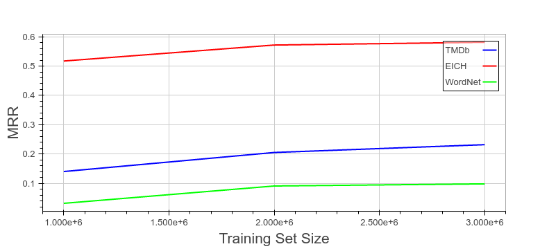
Figure 16: MRR analysis for Entity Retrieval

5.6 Typed Paths Prediction

Finally, to show the possibilities offered by a generalized graph embedding, we present a technique to obtain the target node of a given typed path, using the type of the path and the source node of the same.

A typed path is a sequence of node and edge types that correspond to one path in the graph (in some context, those typed paths are known as traversals):

Definition 5.

A typed path of a generalized graph $G=(V,E,\tau,\mu)$ is a sequence

$$T=t_{1}\overset{r_{1}}{\rightarrow}t_{2}\overset{r_{2}}{\rightarrow}\ldots\overset{r_{q}}{\rightarrow}t_{q+1}$$

where $t_{i}\in\tau(V)$ and $r_{i}\in\tau(E)$. We denote $Tp(G)$ the set of typed paths in $G$.

Definition 6.

We define an application, $Tp$, that associates to each possible typed path in $G$ the set of paths that verify it, such that if $T=t_{1}\overset{r_{1}}{\rightarrow}t_{2}\overset{r_{2}}{\rightarrow}\ldots\overset{r_{q}}{\rightarrow}t_{q+1}$, then for each $\rho\in Tp(T)$, $(t_{1},\dots,t_{q+1})$ is the ordered sequence of node types in $\rho$, and $(r_{1}\dots,r_{q})$ is the ordered sequence of edge types in $\rho$.

Our goal is to obtain the target node of a path, just from the source node representation and the representative vector of the type that such path verifies. In this case we are not removing the paths before performing the embedding because we only pursue a new way to perform long distance queries in graph databases (not prediction tasks). It should be noted that this kind of queries in the current persistence systems are computationally expensive and that, with methods like the presented here, better performance can be reached by sacrificing optimality.

We will define the representative vector of a path as we did before for edges (indeed, edges can be seen as a particular case of types paths with length 1).

Definition 7.

The representative vector of a path, $n_{1}\overset{\rho}{\rightsquigarrow}n_{k}$, is the vector separating the representations of the source node of the path, $\pi(n_{1})$, and the target node of the path, $\pi(n_{k})$. Then:

$$\pi(\rho)=\overrightarrow{\pi(n_{1})\pi(n_{k})}=\pi(n_{k})-\pi(n_{1})$$

The representative vector of a typed path, $T$, is the average vector of all representative vectors of paths of type $T$:

$$\pi(T)=\frac{1}{|Tp(T)|}\sum_{\rho\in Tp(T)}\pi(\rho)$$

Similarly as in the case of edge types, it is possible that some source nodes have not been sampled by the embedding process and thus their representation do not exist. In those cases, such path will not be evaluated.

We have performed typed path entity retrieval experiments using a similar approach as in the edge case. We have filtered target nodes depending on the type of the last element in the node sequence of the path and we have used the MRR metric again. Experiments have been performed on EICH dataset since this dataset represents a more complex schema and allows more complex typed paths queries.

Figure 17 shows some results obtained using the following typed paths (edge types are omitted as they can be directly inferred from the schema in Figure 7):

1. $T1=(Inmaterial\overset{r_{1}}{\rightarrow}DetSubambito\overset{r_{2}}{\rightarrow}Subambito\overset{r_{3}}{\rightarrow}Ambito)$

   It is associated to paths of length 3 and contains information about Ambito nodes (there are 5 of this type in EICH) associated with Inmaterial nodes in the graph.

2. $T2=(Inmaterial\overset{r_{1}}{\rightarrow}Parroquia\overset{r_{2}}{\rightarrow}Canton\overset{r_{3}}{\rightarrow}Provincia)$

   It is associated to paths of length 3 and contains information about Provincia nodes (there are 24 of this type in EICH) associated with Inmaterial nodes in the graph.

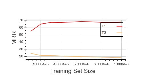
Figure 17: Typed paths MRR Analysis

As Figure 17 shows, this methodology performs well in obtaining the target node of $T1$ paths, obtaining results near to $70\%$ in MRR metric for a training set with more than 3 million pairs. In the case of $T2$, its results tends to be worst when we increase the training set size over a million pairs. The problem associated to $T_{2}$ is more complex, because of the number of Provincia nodes in the graph and the big confusion with this kind of nodes.

We need to perform more tests to validate it, but this application shows that it can be used to approximate long distance queries in databases, a task specially inefficient in classic persistence systems.

6 Conclusions and Future Work

The main goal of this work has been to allow traditional machine learning algorithms to learn from multi-relational data through vector space embedding of generealized graphs, performing automatic feature extraction, and maintaining semantic structures in the obtained representation. We have analysed the different options that a semantic preserving embedding for property graphs (generalized graphs) in vector spaces allows.

If there exists an element (a subgraph) that is immersed in a graph database (a generalized graph), the task of manual feature extraction to characterize it can be very complex. The approximation presented in this work automatically obtains a vectorial representation of such relational data through a sampling of the network information. In this way, this work aliviate the process of feature extraction in multi-relational data and takes into account the global information available during the embedding process.

There are not many works that use neural encoders to perform multi-relational graph embeddings in vector spaces. Our methodology uses simple architectures to obtain vector representations of nodes and edges that maintain (to some extend) the structural and semantic characteristics of the original graph. In addition, it has been experimentally demonstrated that unobserved semantic connections in the original graph (due to lack of information or inconsistency) can be recovered and that it is possible to perform normalization tasks in graph databases or to optimize some kind of queries using our methodology.

Evaluation tests have shown that the accuracy and precision of machine learning algorithms on the new vector representation can inform about the quality of the semantic structure of the dataset. For example, confusion between some nodes / edges in classification tasks can inform about some adjustments to be done in the dataset in order to reflect the semantic characteristics correctly (and to improve classification or prediction tasks). A detailed report about how different node and edge types clusters are overlapping in the new space would be very useful when normalizing graph database data schemas.

The training set and selection window size positively influence the applicability of the obtained embedding, but these facts must be studied in greater depth, since they can be crucial in the automatic tunning of the encoding paremeters.

We have explored how vector structures can be used to retrieve information from generalized graphs, as shown by Entity Retrieval and typed paths experiments. It is likely that looking for complex structures in the projected space will be simpler than in the original one. In fact, the use of a second layer of learning models after neural encoding can improve the results of various tasks related to information retrieval tasks in semantic graphs. Results show that it is worth considering this line of research. Although not enough experiments have been carried out on typed path queries, the results obtained show that executing query time can be reduced dramatically by sacrificing optimality. This type of queries are very expensive in classical databases, and although graph databases help to reduce their computational cost they still present hard efficiency problems when the path to query is longer than 3.

Compared to other approaches in the same direction, this paper presents the novelty of working with more general semantic contexts, and not only with random paths, which suppose a linearisation of the original graph structure. But these are not the only options to carry out generalized graph encodings through neural networks, as future work, we could achieve vectorial encodings by using neural autoencoders, so that the neural encoder will learn the identity function for the elements of the graph, avoiding the bias imposed by the function that relates the elements to their context.

It should be noted that during the revision of this document new tools optimizing word2vec related learning procedures have been published [3]. In spite of the probable improvement that these tools would suppose in our methodology, we have decided not to take them into account since they do not modify the essence of our proposal, although it would alleviate the computational costs associated to the performed experiments.

Efficiency improvements in long-distance queries shown in section 5.6 deserve to be evaluated in greater depth and compared with other similar methods. Some results related to the semantic analysis of generalized graphs have not been presented in this paper although they are expected to be in later works. Options such as sampling the context of edges, performing their embedding and infer from it an embedding for nodes have not been taken into account and can offer interesting results. Even embeddings of the both sets simultaneously should be considered.

Also as a future line of work, to analyse the characteristics of the embeddings should be considered. A first step is about how to construct the training set to be consumed by the neural encoder. In a first approximation the construction of the training set has been totally random, ie, all nodes have the same probability of being sampled, as well as all their properties and neighbours. This may not be the most appropriate way depending on the type of activity to be performed with the obtained embedding. For example, it may be beneficial that nodes with a greater semantic richness are more likely to be in the training set, this option may contribute to explore regions initially less likely to be considered.

It should also be noted that the possibility of working with continuous properties in nodes and edges is open, and should be considered to expand the capacity of our methodology. There are direct mechanisms to include the presence of continuous properties, it remains as work to begin by testing them and to measure later to what extent other approaches can be taken into account.

Similarly, it would be interesting to think about neural encoders that make use of recurrent neural networks to analyse the behaviour of dynamic relational information, an area practically unexplored today.

Table 6: Confusion matrix: Link types prediction (WordNet)

	hyper	dom_reg	part_mero	dom_cat	part_holo	dom_usage	also	memb_mero	inst_hypo	dom_memb_usage	memb_holo	hypo
hyper	83.67%	0.01%	1.14%	0.76%	0.43%	0.02%	0.56%	1.96%	0.13%	0.02%	2.77%	8.52%
dom_reg	2.08%	65.58%	25.0%	0.33%	0.93%	0.0%	0.21%	3.27%	0.24%	0.0%	1.12%	1.25%
part_mero	29.21%	0.74%	44.47%	1.1%	3.54%	0.01%	0.79%	4.12%	0.34%	0.0%	4.47%	11.2%
dom_cat	14.88%	0.02%	1.19%	78.91%	0.11%	0.01%	0.44%	0.18%	0.04%	0.0%	0.25%	3.97%
part_holo	15.53%	0.09%	3.28%	0.34%	45.36%	0.01%	0.78%	2.25%	1.24%	0.0%	6.67%	24.45%
dom_usage	4.28%	0.0%	0.06%	0.39%	0.03%	93.41%	0.99%	0.06%	0.0%	0.0%	0.11%	0.68%
also	8.0%	0.0%	0.38%	0.43%	0.19%	0.03%	78.0%	1.92%	0.07%	0.01%	4.64%	6.35%
memb_mero	11.7%	0.18%	1.76%	0.2%	0.77%	0.0%	0.93%	50.72%	0.21%	0.0%	24.67%	8.87%
inst_hypo	2.47%	0.06%	0.87%	0.05%	1.81%	0.0%	0.2%	0.53%	80.42%	0.0%	1.56%	12.02%
dom_memb_usage	1.1%	0.0%	0.03%	0.03%	0.14%	0.0%	1.13%	0.09%	0.06%	93.62%	0.09%	3.73%
memb_holo	11.24%	0.05%	0.67%	0.09%	1.83%	0.0%	0.91%	14.01%	0.21%	0.0%	62.37%	8.61%
hypo	10.52%	0.01%	0.42%	0.31%	1.18%	0.02%	0.57%	1.23%	1.18%	0.01%	3.67%	80.88%

Table 7: Confusion matrix: Node types prediction (EICH)

	Subambito	Provincia	Comunidad	Anexos	Herramienta	Canton	Lengua	Inmaterial	Ambito	Parroquia	DetalleSubambito
Subambito	14.53%	0.0%	0.0%	2.56%	0.0%	0.0%	0.0%	47.86%	0.0%	0.85%	34.19%
Provincia	0.0%	7.14%	2.04%	0.0%	0.0%	69.39%	5.1%	1.02%	0.0%	15.31%	0.0%
Comunidad	0.0%	0.0%	0.0%	7.91%	0.0%	1.44%	0.0%	25.18%	0.0%	65.47%	0.0%
Anexos	0.0%	0.0%	0.0%	81.16%	0.0%	0.0%	0.0%	18.63%	0.0%	0.21%	0.0%
Herramienta	0.0%	0.0%	0.0%	0.68%	36.99%	0.0%	0.0%	62.33%	0.0%	0.0%	0.0%
Canton	0.0%	3.74%	0.1%	5.27%	0.0%	12.18%	0.0%	24.26%	0.0%	54.27%	0.19%
Lengua	0.0%	0.0%	0.0%	6.25%	0.0%	0.0%	0.0%	21.25%	0.0%	72.5%	0.0%
Inmaterial	0.01%	0.0%	0.0%	9.44%	0.19%	0.0%	0.01%	89.77%	0.0%	0.56%	0.01%
Ambito	44.0%	0.0%	0.0%	0.0%	0.0%	0.0%	0.0%	28.0%	0.0%	0.0%	28.0%
Parroquia	0.02%	0.42%	0.08%	2.34%	0.02%	2.11%	0.35%	29.67%	0.0%	64.82%	0.18%
DetalleSubambito	1.63%	0.0%	0.0%	5.42%	0.0%	0.18%	0.0%	49.37%	0.0%	4.52%	38.88%

Table 8: Confusion matrix: Link types prediction (EICH)

	CANTON_L	COM	LOC	HERRAM	PARROQ_L	ANEXO	SUBAMBITO_P	LENGUA	AMBITO	DSUBAMBITO_P
CANTON_L	25.05%	1.94%	12.62%	0.0%	26.8%	6.99%	0.0%	22.91%	3.69%	0.0%
COM	0.0%	97.92%	0.18%	0.0%	0.09%	0.37%	0.0%	1.4%	0.04%	0.0%
LOC	0.0%	0.12%	96.77%	0.04%	1.08%	1.51%	0.0%	0.33%	0.15%	0.0%
HERRAM	0.0%	0.0%	1.49%	44.03%	2.24%	48.51%	0.0%	3.73%	0.0%	0.0%
PARROQ_L	0.89%	0.99%	13.95%	0.02%	59.11%	3.34%	0.0%	19.2%	2.45%	0.05%
ANEXO	0.14%	0.14%	0.49%	0.02%	2.46%	95.87%	0.0%	0.73%	0.11%	0.05%
SUBAMBITO_P	0.81%	0.0%	10.57%	0.0%	8.13%	9.76%	30.89%	14.63%	5.69%	19.51%
LENGUA	0.0%	1.06%	0.09%	0.0%	0.01%	0.39%	0.0%	98.34%	0.1%	0.0%
AMBITO	0.01%	0.04%	0.28%	0.01%	0.04%	1.9%	0.0%	2.38%	95.33%	0.02%
DSUBAMBITO_P	0.18%	0.18%	1.96%	0.0%	2.67%	3.21%	0.89%	22.46%	7.66%	60.78%

References

- [1] P. Almagro-Blanco and F. Sancho-Caparrini. Generalized Graph Pattern Matching. arXiv e-prints arXiv:1708.03734.
- [2] Yoshua Bengio et al. Learning deep architectures for ai. Foundations and trends® in Machine Learning, 2(1):1–127, 2009.
- [3] Piotr Bojanowski, Edouard Grave, Armand Joulin, and Tomas Mikolov. Enriching word vectors with subword information. arXiv preprint arXiv:1607.04606, 2016.
- [4] Antoine Bordes, Nicolas Usunier, Alberto Garcia-Duran, Jason Weston, and Oksana Yakhnenko. Translating embeddings for modeling multi-relational data. In C. J. C. Burges, L. Bottou, M. Welling, Z. Ghahramani, and K. Q. Weinberger, editors, Advances in Neural Information Processing Systems 26, pages 2787–2795. Curran Associates, Inc., 2013.
- [5] I. Borg and P.J.F. Groenen. Modern Multidimensional Scaling: Theory and Applications. Springer, 2005.
- [6] Kai-Wei Chang, Scott Wen-tau Yih, Bishan Yang, and Chris Meek. Typed tensor decomposition of knowledge bases for relation extraction. In Proceedings of the 2014 Conference on Empirical Methods in Natural Language Processing. ACL – Association for Computational Linguistics, October 2014.
- [7] Shiyu Chang, Wei Han, Jiliang Tang, Guo-Jun Qi, Charu C. Aggarwal, and Thomas S. Huang. Heterogeneous network embedding via deep architectures. In Proceedings of the 21th ACM SIGKDD International Conference on Knowledge Discovery and Data Mining, KDD ’15, pages 119–128, New York, NY, USA, 2015. ACM.
- [8] Michaël Defferrard, Xavier Bresson, and Pierre Vandergheynst. Convolutional neural networks on graphs with fast localized spectral filtering. CoRR, abs/1606.09375, 2016.
- [9] David K Duvenaud, Dougal Maclaurin, Jorge Iparraguirre, Rafael Bombarell, Timothy Hirzel, Alan Aspuru-Guzik, and Ryan P Adams. Convolutional networks on graphs for learning molecular fingerprints. In C. Cortes, N. D. Lawrence, D. D. Lee, M. Sugiyama, and R. Garnett, editors, Advances in Neural Information Processing Systems 28, pages 2224–2232. Curran Associates, Inc., 2015.
- [10] C. Fellbaum. WordNet: An Electronic Lexical Database. Language, speech, and communication. MIT Press, 1998.
- [11] Xavier Glorot, Antoine Bordes, Jason Weston, and Yoshua Bengio. A semantic matching energy function for learning with multi-relational data. CoRR, abs/1301.3485, 2013.
- [12] Aditya Grover and Jure Leskovec. node2vec: Scalable feature learning for networks, 2016. cite arxiv:1607.00653Comment: In Proceedings of the 22nd ACM SIGKDD International Conference on Knowledge Discovery and Data Mining, 2016.
- [13] G E Hinton and R R Salakhutdinov. Reducing the dimensionality of data with neural networks. Science, 313(5786):504–507, July 2006.
- [14] Yann Jacob, Ludovic Denoyer, and Patrick Gallinari. Learning latent representations of nodes for classifying in heterogeneous social networks. In Proceedings of the 7th ACM International Conference on Web Search and Data Mining, WSDM ’14, pages 373–382, New York, NY, USA, 2014. ACM.
- [15] Thomas N Kipf and Max Welling. Semi-supervised classification with graph convolutional networks. arXiv preprint arXiv:1609.02907, 2016.
- [16] Tomas Mikolov, Kai Chen, Greg Corrado, and Jeffrey Dean. Efficient estimation of word representations in vector space. CoRR, abs/1301.3781, 2013.
- [17] Tomas Mikolov, Scott Wen-tau Yih, and Geoffrey Zweig. Linguistic regularities in continuous space word representations. In Proceedings of the 2013 Conference of the North American Chapter of the Association for Computational Linguistics: Human Language Technologies (NAACL-HLT-2013). Association for Computational Linguistics, May 2013.
- [18] Bryan Perozzi, Rami Al-Rfou, and Steven Skiena. Deepwalk: Online learning of social representations. In Proceedings of the 20th ACM SIGKDD International Conference on Knowledge Discovery and Data Mining, KDD ’14, pages 701–710, New York, NY, USA, 2014. ACM.
- [19] Franco Scarselli, Marco Gori, Ah Chung Tsoi, Markus Hagenbuchner, and Gabriele Monfardini. The graph neural network model. IEEE Trans. Neural Networks, 20(1):61–80, 2009.
- [20] Michael Schlichtkrull, Thomas N Kipf, Peter Bloem, Rianne van den Berg, Ivan Titov, and Max Welling. Modeling relational data with graph convolutional networks. arXiv preprint arXiv:1703.06103, 2017.
- [21] Richard Socher, Danqi Chen, Christopher D Manning, and Andrew Ng. Reasoning with neural tensor networks for knowledge base completion. In C. J. C. Burges, L. Bottou, M. Welling, Z. Ghahramani, and K. Q. Weinberger, editors, Advances in Neural Information Processing Systems 26, pages 926–934. Curran Associates, Inc., 2013.
- [22] Jian Tang, Meng Qu, Mingzhe Wang, Ming Zhang, Jun Yan, and Qiaozhu Mei. Line: Large-scale information network embedding. In Proceedings of the 24th International Conference on World Wide Web, WWW ’15, pages 1067–1077, New York, NY, USA, 2015. ACM.
- [23] Bishan Yang, Wen-tau Yih, Xiaodong He, Jianfeng Gao, and Li Deng. Embedding entities and relations for learning and inference in knowledge bases. CoRR, abs/1412.6575, 2014.
- [24] Bishan Yang, Wen-tau Yih, Xiaodong He, Jianfeng Gao, and Li Deng. Learning multi-relational semantics using neural-embedding models. CoRR, abs/1411.4072, 2014.