2017 222 29 August

The ALICE Transition Radiation Detector

ALICE Collaboration ALICE Collaboration

The Transition Radiation Detector (TRD) was designed and built to enhance the capabilities of the ALICE detector at the Large Hadron Collider (LHC). While aimed at providing electron identification and triggering, the TRD also contributes significantly to the track reconstruction and calibration in the central barrel of ALICE. In this paper the design, construction, operation, and performance of this detector are discussed. A pion rejection factor of up to 410 is achieved at a momentum of 1 GeV/$c$ in p–Pb collisions and the resolution at high transverse momentum improves by about 40% when including the TRD information in track reconstruction. The triggering capability is demonstrated both for jet, light nuclei, and electron selection.

1 Introduction

A Large Ion Collider Experiment (ALICE) [1, 2] is the dedicated heavy-ion experiment at the Large Hadron Collider (LHC) at CERN. In central high energy nucleus–nucleus collisions a high-density deconfined state of strongly interacting matter, known as quark–gluon plasma (QGP), is supposed to be created [3, 4, 5]. ALICE is designed to measure a large set of observables in order to study the properties of the QGP. Among the essential probes there are several involving electrons, which originate, e.g. from open heavy-flavour hadron decays, virtual photons, and Drell-Yan production as well as from decays of the $\psi$ and $\rm\Upsilon$ families. The identification of these rare probes requires excellent electron identification, also in the high multiplicity environment of heavy-ion collisions. In addition, the rare probes need to be enhanced with triggers, in order to accumulate the statistics necessary for differential studies. The latter requirement concerns not only probes involving the production of electrons, but also rare high transverse momentum probes such as jets (collimated sprays of particles) with and without heavy flavour. The ALICE Transition Radiation Detector (TRD) fulfils these two tasks and thus extends the physics reach of ALICE.

Transition radiation (TR), predicted in 1946 by Ginzburg and Frank [6], occurs when a particle crosses the boundary between two media with different dielectric constants. For highly relativistic particles ($\gamma\gtrsim 1000$), the emitted radiation extends into the X-ray domain for a typical choice of radiator [7, 8, 9]. The radiation is extremely forward peaked relative to the particle direction [7]. As the TR photon yield per boundary crossing is of the order of the fine structure constant ($\alpha=1/137$), many boundaries are needed in detectors to increase the radiation yield [10]. The absorption of the emitted X-ray photons in high-$Z$ gas detectors leads to a large energy deposition compared to the specific energy loss by ionisation of the traversing particle.

Since their development in the 1970s, transition radiation detectors have proven to be powerful devices in cosmic-ray, astroparticle and accelerator experiments [11, 12, 13, 14, 10, 15, 16, 17, 18, 19, 20]. The main purpose of the transition radiation detectors in these experiments was the discrimination of electrons from hadrons via, e.g. cluster counting or total charge/energy analysis methods. In a few cases they provided charged-particle tracking. The transition radiation photons are in most cases detected either by straw tubes or by multiwire proportional chambers (MWPC). In some experiments [10, 13, 21, 16] and in test setups [22, 23, 24, 25], short drift chambers (usually about $1\text{\,}\mathrm{cm}$) were employed for the detection. Detailed reviews on the transition radiation phenomenon, detectors, and their application to particle identification can be found in [10, 26, 27, 28].

The ALICE TRD, which covers the full azimuth and the pseudorapidity range $-0.84<\eta<0.84$ (see next section), is part of the ALICE central barrel. The TRD consists of 522 chambers arranged in 6 layers at a radial distance from $2.90\text{\,}\mathrm{m}$ to $3.68\text{\,}\mathrm{m}$ from the beam axis. Each chamber comprises a foam/fibre radiator followed by a Xe-CO₂-filled MWPC preceded by a drift region of $3\text{\,}\mathrm{cm}$. The extracted temporal information represents the depth in the drift volume at which the ionisation signal was produced and thus allows the contributions of the TR photon and the specific ionisation energy loss of the charged particle $\mathrm{d}E/\mathrm{d}x$ to be separated. The former is preferentially absorbed at the entrance of the chamber and the latter distributed uniformly along the track. Electrons can be distinguished from other charged particles by producing TR and having a higher $\mathrm{d}E/\mathrm{d}x$ due to the relativistic rise of the ionisation energy loss. The usage of the temporal information further enhances the electron-hadron separation power. Due to the fast read-out and online reconstruction of its signals, the TRD has also been successfully used to trigger on electrons with high transverse momenta and jets (3 or more high-$p_{\mathrm{T}}$ tracks). Last but not least, the TRD improves the overall momentum resolution of the ALICE central barrel by providing additional space points at large radii for tracking, and tracks anchored by the TRD will be a key element to correct space charge distortions expected in the ALICE TPC in LHC Run 3 [29]. A first version of the correction algorithm is already in use for Run 2.

In this article the design, construction, operation, and performance of the ALICE TRD is described. Section 2 gives an overview of the detector and its construction. The gas system is detailed in Section 3. The services required for the detector are outlined in Section 4. In Section 5 the read-out of the detector is discussed and the Detector Control System (DCS) used for reliable operation and monitoring of the detector is presented in Section 6. The detector commissioning and its operation are discussed in Section 7. Tracking, alignment, and calibration are described in detail in Sections 8, 9, and 10, while various methods for charged hadron and electron identification are presented in Section 11. The use of the TRD trigger system for jets, electrons, heavy-nuclei, and cosmic-ray muons is described in Section 12.

2 Detector overview

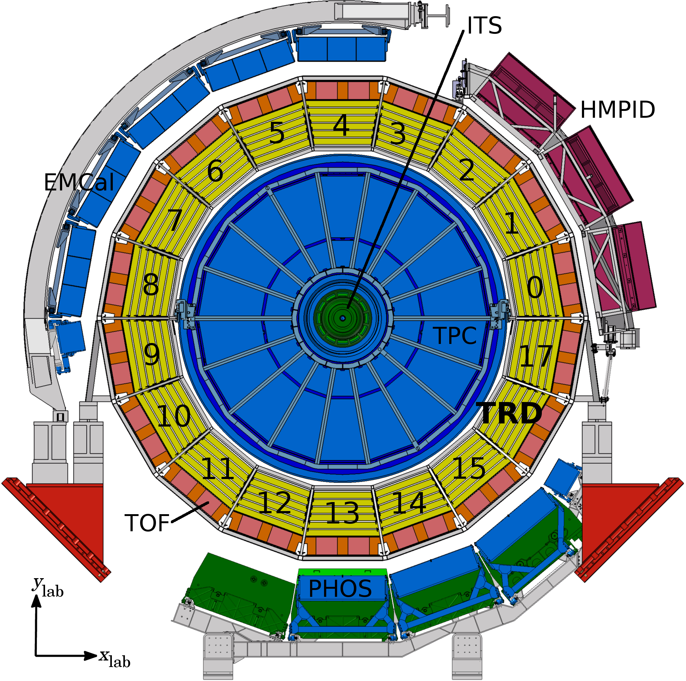
Figure 1: Schematic cross-section of the ALICE detector perpendicular to the LHC beam direction (status of the detector since the start of LHC Run 2). The central barrel detectors cover the pseudorapidity range $|\eta|\lesssim 0.9$ and are located inside the solenoid magnet, which provides a magnetic field with strength $B$ = $0.5\text{\,}\mathrm{T}$ along the beam direction.

A cross-section of the central part of the ALICE detector [1, 2], installed at Interaction Point 2 (IP2) of the LHC, is shown in Fig. 1. The central barrel detectors cover the pseudorapidity range $|\eta|\lesssim 0.9$ and are located inside a solenoid magnet, which produces a magnetic field of $B$ = $0.5\text{\,}\mathrm{T}$ along the beam direction. The Inner Tracking System (ITS) [30], placed closest to the nominal interaction point, is employed for low momentum tracking, particle identification (PID), and primary and secondary vertexing. The Time Projection Chamber (TPC) [31], which is surrounded by the TRD, is used for tracking and PID. The Time-Of-Flight detector (TOF) [32] is placed outside the TRD and provides charged hadron identification. The ElectroMagnetic Calorimeter (EMCal) [33], the PHOton Spectrometer (PHOS) [34], and the High Momentum Particle Identification Detector (HMPID) [35] are used for electron, jet, photon and hadron identification. Their azimuthal coverage is shown in Fig. 1. Not visible in the figure are the V0 and T0 detectors [36, 37], as well as the Zero Degree Calorimeters (ZDC) [38], which are placed at small angles on both sides of the interaction region. These detectors can be employed, e.g. to define a minimum-bias trigger, to determine the event time, the centrality and event plane of a collision [2, 39, 40]. Likewise, the muon spectrometer [41, 42] is outside the view on one side of the experiment, only, covering $-$4 $<\eta<$ $-$2.5.

Figure 1 also shows the definition of the global ALICE coordinate system, which is a Cartesian system with its point of origin at the nominal interaction point ($x_{\rm lab}$, $y_{\rm lab}$, $z_{\rm lab}$ = 0); the $x_{\rm lab}$-axis pointing inwards radially to the centre of the LHC ring and the $z_{\rm lab}$-axis coinciding with the direction of one beam and pointing in direction opposite to the muon spectrometer. According to the (anti-)clock-wise beam directions, the muon spectrometer side is also called C-side, the opposite side A-side.

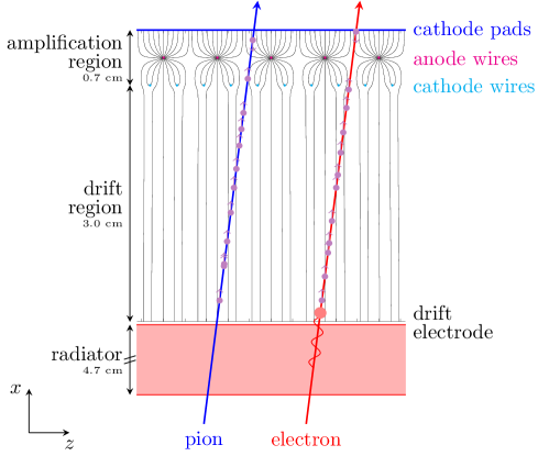
Figure 2: Schematic cross-section of a TRD chamber in the $x$-$z$ plane (perpendicular to the wires) with tracks of a pion and an electron to illustrate the ionisation energy deposition and the TR contribution. The large energy deposition due to the TR photon absorption is indicated by the large red circle in the drift region. The drift lines (solid lines) are calculated with Garfield [43] and correspond to the nominal voltage settings for chamber operation. The radiator is not drawn to scale.

The design of the TRD is a result of the requirements and constraints discussed in the Technical Design Report [44]. It has a modular structure and its basic component is a multiwire proportional chamber (MWPC). Each chamber is preceded by a drift region to allow for the reconstruction of a local track segment, which is required for matching of TRD information with tracks reconstructed with ITS and TPC at high multiplicities. TR photons are produced in a radiator mounted in front of the drift section and then absorbed in a xenon-based gas mixture. A schematic cross-section of a chamber and its radiator is shown in Fig. 2. The shown local coordinate system is a right-handed orthogonal Cartesian system, similar to the global coordinate system, rotated such that the $x$-axis is perpendicular to the chamber. Six layers of chambers are installed to enhance the pion rejection power. An eighteen-fold segmentation in azimuth ($\varphi$), with each segment called ‘sector’, was chosen to match that of the TPC read-out chambers. In the longitudinal direction ($z_{\rm lab}$), i.e. along the beam direction, the coverage is split into five stacks, resulting in a manageable chamber size. The five stacks are numbered from 0 to 4, where stack 4 is at the C-side and stack 0 at the A-side. Layer 0 is closest, layer 5 farthest away from the collision point in the radial direction. In each sector, 30 read-out chambers (arranged in 6 layers and 5 stacks) are combined in a mechanical casing, called a ‘supermodule’ (see Fig. 3 and Section 2.3).

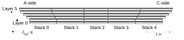
Figure 3: Cross-section (longitudinal view) of a supermodule.

In total the TRD can host 540 read-out chambers (18 sectors $\times$ 6 layers $\times$ 5 stacks), however in order to minimise the material in front of the PHOS detector in three sectors (sectors 13–15, for numbering see Fig. 1) the chambers in the middle stack were not installed. This results in a system of 522 individual read-out chambers. The main parameters of the detector are summarised in Table 1.

Parameter	Value
Pseudorapidity coverage	$-$0.84 $<\eta<$ +0.84
Azimuthal coverage $\varphi$	$360\mathrm{°}$
Radial position	$2.90\text{\,}\mathrm{m}3.68\text{\,}\mathrm{m}$
Length of a supermodule	$7.02\text{\,}\mathrm{m}$
Weight of a supermodule	$1.65\text{\,}\mathrm{t}$
Segmentation in $\varphi$	18 sectors
Segmentation in $z_{\rm lab}$	5 stacks
Segmentation in $r$	6 layers
Total number of read-out chambers	522
Size of a read-out chamber (active area)	$0.90\text{\,}\mathrm{m}$ $\times$ $1.06\text{\,}\mathrm{m}$ to $1.13\text{\,}\mathrm{m}$ $\times$ $1.43\text{\,}\mathrm{m}$
Radiator material	fibre/foam sandwich
Depth of radiator	$4.7\text{\,}\mathrm{cm}$
Depth of drift region	$3.0\text{\,}\mathrm{cm}$
Depth of amplification region	$0.7\text{\,}\mathrm{cm}$
Number of time bins ($100\text{\,}\mathrm{ns}$)	30 (22–24)
Total number of read-out pads	$1\,150\,848$
Total active area	$673.4\text{\,}{\mathrm{m}}^{2}$
Detector gas	Xe-CO2 (85-15)
Gas volume	$27\text{\,}{\mathrm{m}}^{3}$
Drift voltage (nominal)	${\sim}$$2150\text{\,}\mathrm{V}$
Anode voltage (nominal)	${\sim}$$1520\text{\,}\mathrm{V}$
Gas gain (nominal)	${\sim}3200$
Drift field	${\sim}$$700\text{\,}\mathrm{V}\mathrm{/}\mathrm{c}\mathrm{m}$
Drift velocity	${\sim}$$1.56\text{\,}\mathrm{c}\mathrm{m}\mathrm{/}\mathrm{\SIUnitSymbolMicro}\mathrm{s}$
Avg. radiation length along $r$ $\langle X/X_{0}\rangle$	24.7%

Table 1: General parameters of the TRD. The indicated weight corresponds to a supermodule with 30 read-out chambers; the length of the supermodule does not include the connected services. At maximum 30 time bins can be read out, typical values used in Run 1 and Run 2 are 22–24 (see Section 5.2).

At the start of the first LHC period (Run 1) in 2009 the TRD participated with seven supermodules. Six further supermodules were built and integrated into the experiment during short winter shutdown periods of the accelerator, three in each winter shutdown period of 2010 and 2011. The TRD was completed during the Long Shutdown 1 (LS) of the LHC in 2013–2014. With all 18 supermodules installed, full coverage in azimuth was accomplished for the second LHC period (Run 2) starting in 2015.

2.1 Read-out chambers

The size of the read-out chambers changes radially and along the beam direction (see Fig. 3). The active area per chamber thus varies from $0.90\text{\,}\mathrm{m}$ $\times$ $1.06\text{\,}\mathrm{m}$ to $1.13\text{\,}\mathrm{m}$ $\times$ $1.43\text{\,}\mathrm{m}$ ($x\times z$). The optimal design of a read-out chamber (see Fig. 2) was found considering the requirements on precision and mechanical stability, and minimisation of the amount of material.

The construction of the radiator, discussed in the following sub-section, is essential for the mechanical stability of the chamber. The drift electrode, an aluminised mylar foil ($25\text{\,}\mathrm{\SIUnitSymbolMicro m}$ thick), is an integral part of the radiator. To ensure a uniform drift field throughout the entire drift volume, a field cage with a voltage divider chain is employed [44]. The current at nominal drift voltage is about $170\text{\,}\mathrm{\SIUnitSymbolMicro A}$. The grounded cathode wires are made of Cu-Be and have a diameter of $75\text{\,}\mathrm{\SIUnitSymbolMicro m}$, while the anode wires are made of Au-plated tungsten with a diameter of $20\text{\,}\mathrm{\SIUnitSymbolMicro m}$. The pitch for the cathode and anode wires are $2.5\text{\,}\mathrm{mm}$ and $5\text{\,}\mathrm{mm}$, respectively; the tensions at winding were $1\text{\,}\mathrm{N}$ and $0.45\text{\,}\mathrm{N}$ [45]. The wire lengths vary from $1.08\text{\,}\mathrm{m}$ to $1.45\text{\,}\mathrm{m}$. The maximum deformation of the chamber frame was $150\text{\,}\mathrm{\SIUnitSymbolMicro m}$ under the wire tension indicated, leading to a maximum 10% loss in wire tension. Even with an additional $1\text{\,}\mathrm{mbar}$ overpressure in the gas volume (see Section 3), the deformation of the drift electrode can be kept within the specification of less than $1\text{\,}\mathrm{mm}$. The segmented cathode pad plane is manufactured from thin Printed Circuit Boards (PCB) and glued on a light honeycomb and carbon fibre sandwich to ensure planarity and mechanical stiffness. The design goal of having a maximum deviation from planarity of $150\text{\,}\mathrm{\SIUnitSymbolMicro m}$ was achieved with only a few chambers exceeding slightly this value. The PCBs of the pad plane were produced in two or three pieces. The PCBs are segmented into 12 (stack 2) or 16 pads along the $z$-direction, and 144 pads in the direction of the anode wires ($r\varphi$). The pad area varies from $0.635\text{\,}\mathrm{cm}$ $\times$ $7.5\text{\,}\mathrm{cm}$ to $0.785\text{\,}\mathrm{cm}$ $\times$ $9\text{\,}\mathrm{cm}$ [45] to achieve a constant granularity with respect to the distance from the interaction point. The pad width of $0.635\text{\,}\mathrm{cm}$ to $0.785\text{\,}\mathrm{cm}$ in the $r\varphi$ direction was chosen so that charge sharing between adjacent pads (typically three), which is quantified by the pad response function (PRF) [46], is achieved. As a consequence, the position of the charge deposition can be reconstructed in the $r\varphi$-direction with a spatial resolution of $\lesssim$ $400\text{\,}\mathrm{\SIUnitSymbolMicro m}$ [46]. In the longitudinal direction, the coarser segmentation is sufficient for the track matching with the inner detectors. In addition, the pads are tilted by $\pm$ $2\mathrm{°}$ (sign alternating layer-by-layer) as shown in Fig. 4, which improves the $z$-resolution during track reconstruction without compromising the $r\varphi$ resolution. For clusters confined within one pad row, a $z$ position at the row centre is assumed, $z_{\rm cluster}=z_{0}$. The honeycomb structure also acts as a support for the read-out boards. The pads are connected to the read-out boards by short polyester ribbon cables via milled holes in the honeycomb structure.

The original design of the TRD was conceived such that events with a multiplicity of d$N_{\rm ch}$/d$\eta$ = $8000$ would have lead to an occupancy of 34% in the detector [44]. The fast read-out and processing of such data on $1.15\cdot 10^{6}$ read-out channels required the design and production of fully customised front-end electronics (see Section 5).

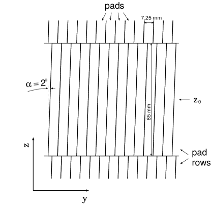
Figure 4: Pad geometry of a TRD read-out chamber in layer 3 (not stack 2). The pad tilt is $\pm$ $2\mathrm{°}$ with respect to the $z$-axis (along the beam direction), with the sign alternating between layers.

Figure 5: Average pulse height as a function of drift time for pions and electrons (with and without radiator). The time axis is shown with an arbitrary offset of $0.3\text{\,}\mathrm{\SIUnitSymbolMicro s}$. The measurements were performed at the CERN PS with prototype read-out chambers that were smaller in overall size (active area $25\text{\,}\mathrm{cm}$ $\times$ $32\text{\,}\mathrm{cm}$) but otherwise similar in construction to that of the final detector. Figure taken from [47].

The positive signal induced on the cathode pad plane is amplified using a charge-sensitive PreAmplifier-ShAper (PASA) (see Section 5) and the signals on the cathode pads are sampled in time bins of 100 ns inside the TRAcklet Processor (TRAP, see Section 5). For LHC Run 1 and Run 2 running conditions (see Section 7.2), the probability for pile-up events is small. The averaged time evolution of the signal is shown in Fig. 5 for pions and electrons, with and without radiator. In the amplification region (early times), the signal is larger, because the ionisation from both sides of the anode wires contributes to the same time interval. The contribution of TR is seen as an increase in the measured average signal at times corresponding to the entrance of the chamber (around $2.5\text{\,}\mathrm{\SIUnitSymbolMicro s}$ in Fig. 5), where the TR photons are preferentially absorbed. At large times (beyond $2.5\text{\,}\mathrm{\SIUnitSymbolMicro s}$), the effect of the slow ion movement becomes visible as a tail. Various approximations of the time response function, the convolution of the long tails with the shaping of the PASA, were studied in order to optimally cancel the tails in data, see Section 8.

Figure 6: Distributions of the ionisation energy loss of pions and electrons with momenta of 2 $\mathrm{GeV}\!/c$. The symbols represent the measurements obtained at the CERN PS with prototype read-out chambers that were smaller in overall size (active area  $25\text{\,}\mathrm{cm}$ $\times$ $32\text{\,}\mathrm{cm}$) but otherwise similar in construction to that of the final detector. The lines are simulations accounting (continuous line) or not (dashed line) for the long range of $\delta$-electrons as compared to the chamber dimensions. Figure taken from [48].

The knowledge of the ionisation energy loss is important for the control of the detector performance and for tuning the Monte Carlo simulations. A set of measurements was performed with prototype read-out chambers with detachable radiators for pions and electrons at various momenta [48]. An illustration of the measured data is shown in Fig. 6 for pions and electrons with a momentum of 2 $\mathrm{GeV}\!/c$. The simulations describe the Landau distribution of the total ionisation energy deposition, determined from the calibrated time-integrated chamber signal. A compilation of such measurements over a broad momentum range including data obtained with cosmic-ray muons and from collisions recorded with ALICE is shown in Section 11, Fig. 37.

Measurements of the position resolution in the $r\varphi$-direction ($\sigma_{y}$) and angular resolution $\sigma_{\varphi}$, conducted with prototype chambers, established that the required performance of the detector and electronics ($\sigma_{y}$ $\lesssim$$400\text{\,}\mathrm{\SIUnitSymbolMicro m}$ and $\sigma_{\varphi}$ $\leq$ $1\mathrm{°}$) is reached for signal-to-noise values of about 40, which corresponds to a moderate gas gain of about 3500 [46].

The production of a chamber was performed in several steps [49] and completed in one week on average. First, the aluminium walls of the chamber were aligned on a precision table and glued to the radiator panel. The glueing table was custom-built to ensure the required mechanical precision and time-efficient handling of the components. For almost all junctions the two-component epoxy glue Araldite^® AW 116 with hardener HV 953BD was used. In a few places, where a higher viscosity glue was needed, Araldite^® AW 106 was applied. In a second step, the cathode and anode wires were wound on a custom-made winding machine and glued onto a robust aluminium frame in order to keep the wire tension. This aluminium frame was subsequently placed on top of the chamber body, and the cathode and anode wires were transferred to the G10 ledges glued to the chamber body. After gluing of the anode and cathode wire planes, the tension of each wire was checked by moving a needle valve with pressurised air across the wires. The induced resonance frequency in each wire was determined by measuring the reflected light of an LED [50]. Afterwards the pad plane and honeycomb structure were placed on top of the chamber body. Following this production process, each chamber was subjected to a series of quality control tests with an Ar-CO₂ (70-30) gas mixture. The tests were performed once before the chamber was sealed with epoxy (closed with clamps) and repeated after chamber validation and glueing. In the following the requirements are described [51]. The anode leakage current was required not to exceed a value of 10 nA. The gas leak rate was determined by flushing the chamber with the Ar-CO₂ gas mixture and measuring the O₂ content of the outflowing gas. It was required to be less than $1\text{\,}\mathrm{mbar}$ $\cdot$ $\mathrm{l}\mathrm{/}\mathrm{h}$. In addition, the leak conductance was measured at an underpressure of 0.4–$0.5\text{\,}\mathrm{mbar}$ in the chamber. The underpressure test was only introduced at a later stage of the mass production after viscous leaks were found, see Section 3.4.1 for more details. Comparisons of the anode current induced by a ¹⁰⁹Cd source placed at 100 different positions across the active area allowed determinations of the gain uniformity. The step size for this two-dimensional scan was about 10 cm in both directions and the measured values were required to be within $\pm$ 15% of the median. Electrically disconnected wires were detected by carrying out a one-dimensional scan perpendicular to the wires with a step size of $1\text{\,}\mathrm{cm}$. This scan clearly identified any individual wire that was not connected due to the visible gas gain anomaly in the vicinity of this wire, and allowed for repair. For one position the absolute gas gain was determined by measuring the anode current and by counting the pulses of the ¹⁰⁹Cd source. The long term stability was characterised by monitoring the gas gain in intervals of 15 minutes over a period of 12 hours.

2.2 Radiator

Figure 7: Side (left) and top (right) view of the design of the TRD sandwich radiator [44].

The design of the radiator is shown in Fig. 7. Polypropylene fibre mats of $3.2\text{\,}\mathrm{cm}$ total thickness are sandwiched between two plates of Rohacell^® foam HF71, which are mechanically reinforced by lamination of carbon fibre sheets of $100\text{\,}\mathrm{\SIUnitSymbolMicro m}$ thickness. Aluminised kapton foils are glued on top, to ensure gas tightness and to also serve as the drift electrode. For mechanical reinforcement, cross-bars of Rohacell^® foam of $0.8\text{\,}\mathrm{cm}$ thickness are glued between the two foam sheets of the sandwich, with a pitch of 20–$25\text{\,}\mathrm{cm}$ depending on the chamber size. After construction the transmission of the full radiator was measured using the K_α line of Cu at $8.04\text{\,}\mathrm{keV}$ to ensure the homogeneity of the radiators [52]. This line was chosen as its energy is close to the most probable value of the TR spectrum (see Fig. 8).

Measurements with prototypes [53] indicated that such a sandwich radiator produces 30–40% less TR compared to a regularly spaced foil radiator. However, constructing a large-area detector with radiators made out of 100 regularly spaced foils each is infeasible. The impact of various radiators constructed from fibres and/or foam on, e.g. particle identification is discussed in [53, 47]. Based on these measurements the fibre/foam sandwich radiator design was chosen for the final detector.

Figure 8: Measured and simulated spectra of TR produced by electrons with a momentum of 2 $\mathrm{GeV}\!/c$ for the ALICE TRD sandwich radiator. Figure adapted from [53].

The spectra of TR produced by electrons with a momentum of 2 $\mathrm{GeV}\!/c$ as measured with the ALICE TRD sandwich radiator is shown in Fig. 8. Such a measurement is important for the tuning of simulations in the ALICE setup. As the production of TR is not included in GEANT3 [54], which is used to propagate generated particles through the ALICE apparatus for simulations, we have explicitly added it to our simulations in AliRoot [55], the ALICE offline framework for simulation, reconstruction and analysis. An effective parameterisation of the irregular radiator in terms of a regular foil radiator is employed as an approximation. The simulations describe the data satisfactorily including the momentum dependence [53].

2.3 Supermodule

The detector is installed in the spaceframe (the common support structure for most of the central barrel detectors) in 18 supermodules, each of which can host 30 read-out chambers arranged in 5 stacks and 6 layers (see Fig. 3). The overall shape of the supermodule is a trapezoidal prism with a length of $7.02\text{\,}\mathrm{m}$ ($8\text{\,}\mathrm{m}$ including services). Its height is $0.78\text{\,}\mathrm{m}$ and the shorter (longer) base of the trapezoid is $0.95\text{\,}\mathrm{m}$ ($1.22\text{\,}\mathrm{m}$). The weight of a supermodule with 30 read-out chambers is about $1.65\text{\,}\mathrm{t}$. Mechanical stability is provided by a hull of aluminium profiles and sheets, connected with stainless steel screws. The materials were chosen to minimise the interference with the magnetic field in the solenoid magnet. In front of PHOS, where minimal radiation length is required, the aluminium sheets of the short and long base of the trapezoid were replaced by carbon-fibre windows.

All service connections must be routed internally to the end-caps of the supermodule. Those that require materials with large radiation length are placed at the sidewalls, outside the active area of the TRD and most other detectors in ALICE. This includes the low-voltage power distribution bus bars as well as other copper wires for the Detector Control System (DCS) board power, network and high-voltage (HV) connections between the fanout boxes and read-out chambers, and the rectangular cooling pipes (see Section 4 for more details).

Low-voltage (LV) power for the read-out boards is provided via copper power bus bars (2 for each layer and voltage as described in Table 3) with a cross-section of $6\text{\,}\mathrm{mm}$ $\times$ $6\text{\,}\mathrm{mm}$ (per channel) running along the sidewalls of the supermodule. Each read-out board is connected directly to the power bus bars. Heat generated by ohmic losses in the power bus bars is partially transferred to the adjacent cooling pipes (see Section 4.2). The power bus bars protrude about $30\text{\,}\mathrm{cm}$ from each side of the supermodule hull, where they are equipped with capacitors for voltage stabilisation. On one end-cap of the supermodule the power-bus bars are connected via a low-voltage patch panel to the long supply lines to the power supplies outside of the magnet.

Each read-out chamber is equipped with 6 or 8 read-out boards (see Section 2.1) and one DCS board (see Section 4.4). Power is provided and controlled separately for each DCS board by a power distribution box. The DCS boards are connected via twisted-pair cables to Ethernet patch panels at the end-caps and the boards of two adjacent layers are connected via flat-ribbon cables in a daisy chain loop to provide low-level Joint Test Action Group (JTAG) access to neighbouring boards.

For each chamber, three optical fibres are routed to the end-cap on the C-side. Two fibres connect the optical read-out interfaces to a patch panel, where they are linked via the Global Tracking Unit (GTU) (see Section 5) to the Data AcQuisition (DAQ) systems. One trigger fibre connects the DCS board to the trigger distribution box (see Section 5.1), which receives the trigger signals from the pretrigger system or its back-up system and splits them into 30 fibres (+ 2 spares).

The supermodules were constructed from 2006 to 2014. In the following, we discuss the sequence of required steps. After the construction of the supermodule hulls, the power bus bars and patch panels for the distribution of low voltage for the read-out boards and the cooling bars for the water cooling were mounted on the sidewalls. Next the power distribution box (DCS board power), the box for trigger signal distribution, a patch panel for the optical read-out fibres, and the high-voltage distribution boxes were installed at the end-caps.

Before integrating the read-out chambers into a supermodule, they were equipped with electronics (read-out boards, DCS boards) and cooling pipes. After a series of tests were performed to ensure stable operation [56, 57], the chambers were then inserted layer by layer. The first connection established during the installation was the gas link between the chambers (using polyether ether ketone connectors). The chambers were fixed to the hull with three screws on each of the long sides after performing a manual physical alignment. As demonstrated by later measurements (Section 9), the alignment in $r\varphi$ between the chambers is of the order of 0.6–$0.7\text{\,}\mathrm{mm}$ (r.m.s.).

The cables to and from the read-out boards used for JTAG, low-voltage sensing, Ethernet, and DCS power were routed along one side of the chambers. The cable lengths in the active area on top of the chambers were minimised, avoiding cables from the read-out pads to cross. On the other side of the chambers, only the high voltage cables were routed. They were soldered at two separate HV distribution boxes for anode and drift voltage at one end-cap of the supermodule. Each read-out board (38 per layer) was connected to the power bus bars (low voltage) using pre-mounted cables. The cooling pipes (4 per read-out board) were connected by small Viton tubes. In the $z$-direction across the read-out chambers, only optical fibres for the trigger distribution (1 per chamber) and data read-out (2 per chamber) were routed.

In addition to layer-wise tests during installation, a final test was done after completion. The test setup consisted of low-voltage and high-voltage supplies, a cooling plant, a gas system [58], as well as a full trigger setup and read-out equipment. Also a trigger for cosmic rays was built and installed [59, 60]. It was used for first measurements of the gas gain and the chamber alignment, and to also study the zero suppression during assembly [61, 62, 50, 63, 64, 65].

After transport to CERN pre-installation tests were performed (see Section 7.1 and [66]) and the supermodules were installed in the space frame with a precision of $1\text{\,}\mathrm{cm}$ (r.m.s.) in $z_{\rm lab}$-direction. The maximum tolerance in $\varphi$ is $2\text{\,}\mathrm{cm}$ due to constraints given by the space frame.

In addition to the sequential assembly and installation, four supermodules were completely disassembled again in 2008 and 2009. The initial tests were not sensitive to viscous leaks of the read-out chambers and thus the supermodules were rebuilt after improving the gas tightness (see Section 3.4.1). Furthermore, in 2013 during LS 1, one supermodule was disassembled in order to improve the high-voltage stability of the read-out chambers (see Section 7.3).

2.4 Material budget

A precise knowledge of the material budget of the detector is important to obtain a precise description of the detector in the Monte Carlo simulations, which are used, e.g. to compute the track reconstruction efficiencies.

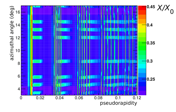
Figure 9: The radiation length map in units of $X/X_{0}$ in a zoomed-in part of the active detector area as a function of the pseudorapidity and the azimuthal angle, calculated from the geometry in AliRoot (the colour scale has a suppressed zero). The positions of the MCMs and the cooling pipes are visible as hot spots. The radiation length was calculated for particles originating from the collision vertex. Therefore the cooling pipes of the six layers overlap for small, but not large $\eta$.

The TRD geometry, as implemented in the simulation part of AliRoot, consists of the read-out chambers, the services, and the supermodule frame. All these parts are placed inside the space frame volume. The material of a read-out chamber is obtained including several material components. A general overview of the various components is given in Table 2.

Description	$\textit{X}/\textit{X}_{0}$ (%)
Radiator	0.69
Chamber gas and amplification region	0.21
Pad plane	0.77
Electronics (incl. honeycomb structure)	1.18
Total	2.85

Table 2: Parts of one read-out chamber, radiator, electronics, and their average contribution to the radiation length in the active area for particles with normal incidence.

The material budget in the simulation was adjusted to match the estimate based on measurements during the construction phase of the final detector. The supermodule frames consist of the aluminium sheets on the sides, top, and bottom of a supermodule together with the traversing support structures, such as the LV power bus bars and cooling arteries. Additional electronics equipment is represented by aluminium boxes that contain the corresponding copper layers to mimic the present material. The services are also introduced, including, e.g. the gas distribution boxes, cooling pipes, power and read-out cables, and power connection panels.

Figure 9 shows the resulting radiation length map, quantified in units of radiation length ($X/X_{0}$), in a zoomed-in part of the active detector area. It is clearly visible that the Multi-Chip Modules (MCM)s on the read-out boards (see Section 5) and the cooling pipes introduce hot spots in $X/X_{0}$. After averaging over the shown area, the mean value is found to be $\langle X/X_{0}\rangle=$ 24.7% for a supermodule with aluminium profiles and sheets and 30 read-out chambers (6 chambers per stack with the material budget as indicated in Table 2). The reduced material budget of the supermodules in front of the PHOS detector (carbon fibre inserts instead of aluminium sheets and no read-out chambers in stack 2) is likewise modelled in the simulation. In regions directly in front of PHOS $\langle X/X_{0}\rangle$ is only 1.9%.

The total weight of a single fully equipped TRD supermodule as described in the AliRoot geometry, including all services, is $1595\text{\,}\mathrm{kg}$, which is about 3.3% less than its real weight. This discrepancy can be attributed to material of service components, such as the gas manifold (see Section 3.3) and the patch panel, outside the active area, which were not introduced in the AliRoot geometry.

3 Gas

At atmospheric pressure, a total of $27\text{\,}{\mathrm{m}}^{3}$ of a xenon-based gas mixture must be circulated through the TRD detector. This expensive gas cannot be flushed through, but rather has to be re-circulated in a closed loop by using a compressor and independent pressure and flow regulation systems. The gas system of the TRD follows a pattern in construction, modularisation, control, and supervision which is common to all LHC gaseous detectors, with emphasis on the regulation of a very small overpressure on the read-out chambers and on the minimisation of leaks. The basic modules such as mixer, purification, pump, exhaust, analysis, etc., are based on a set of equal templates applied to the hardware and the software. A Programmable Logic Controller (PLC) controls each system and the user interacts with it through a supervision panel. Upon a global command, the PLC executes a sequence that configures all elements of the gas system for a given operation mode and continuously regulates the active elements of the system. In this manner the modules and operational conditions can be customised to the specific requirements of each detector, from the control of the stability of the overpressure in the detectors, the circulation flow, and the gas purification, recuperation and distillation, to the monitoring of the gas composition and quality (Xe-CO₂ (85-15), and as little O₂, H₂O and N₂ as possible).

3.1 Gas choice

As well as being an array of tracking drift chambers, the TRD is an electron identification device, achieved through the detection of TR photons. In order to efficiently absorb these several keV photons, a high $Z$ gas is necessary. Figure 10 shows, for three noble gases, the absorption length of photons of energies in the range of typical TR production. At around $10\text{\,}\mathrm{keV}$ the absorption length in Xe is less than a $\mathrm{cm}$, whereas for Kr it is several cm. This argues for the choice of Xe as noble gas for the operating mixture. CO₂ is selected as the quenching gas, since hydrocarbons are excluded for flammability and ageing reasons. The choice of the exact composition is in this case rather flexible, since the design of the wire chambers leaves enough freedom in the choice of the drift field and anode potential. The best compromise for the CO₂ concentration corresponds to the mixture Xe-CO₂ (85-15), which ensures a very good efficiency of TR photon absorption by Xe and provides stability against discharges to the detector.

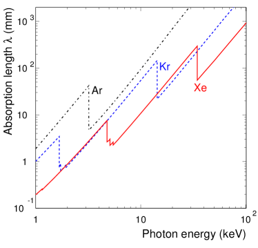
Figure 10: Absorption length of X-rays in noble gases in the relevant energy range of TR production.

Furthermore, this mixture exhibits a nice stability of the drift velocity, at the nominal drift field, also with the inevitable contamination of small amounts of N₂ that accumulates in the gas through leaks (see Section 3.2).

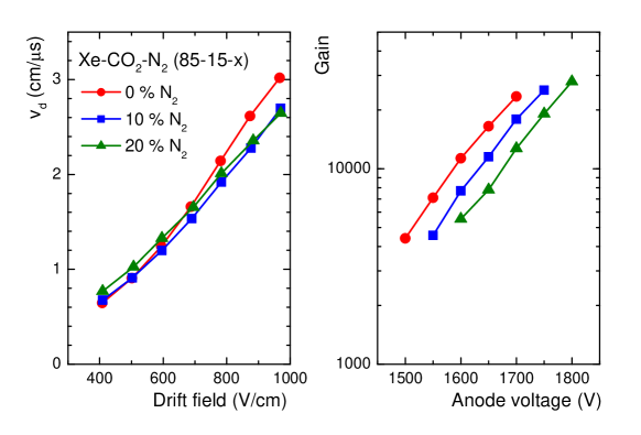
Figure 11: Left: Drift velocity as a function of the drift field for the nominal gas mixture Xe-CO₂ and different admixtures of N₂. Right: Gain as a function of the anode voltage for the same gas mixtures.

The drift velocity of the Xe-CO₂ (85-15) mixture, pure and with substantial admixtures of N₂, as a function of the drift field, is shown in Fig. 11 (left). The drift velocity does not depend on the N₂ contamination at the nominal drift field of $700\text{\,}\mathrm{V}\mathrm{/}\mathrm{c}\mathrm{m}$. On the other hand, as illustrated in Fig. 11 (right), the anode voltage would need a $50\text{\,}\mathrm{V}$ readjustment to keep the gain constant when increasing the concentration of N₂ by 10% in the mixture. It should be noted that intakes of less than 5% N₂ are typically observed in one year of operation. After 2–3 years of operation, the N₂ is cryogenically separated from the Xe (see Section 3.3.9).

The operation of the chambers in a magnetic field of $0.5\text{\,}\mathrm{T}$, perpendicular to the electric drift field ($700\text{\,}\mathrm{V}\mathrm{/}\mathrm{c}\mathrm{m}$), forces the drifting electrons on a trajectory, which is inclined with respect to the electric field. The so-called Lorentz angle is about $9\text{\,}\mathrm{\SIUnitSymbolDegree}$ for this gas mixture (see Section 10).

For commissioning purposes, where TR detection is not necessary, the read-out chambers are flushed with Ar-CO₂ (82-18), which is available in a premixed form at low cost.

3.2 Requirements and specifications

The TRD consists of read-out chambers with an area of about $1\text{\,}{\mathrm{m}}^{2}$ which are built with low material budget. This poses a severe restriction on the maximum overpressure that the detector can hold. Therefore, while in operation, the pressure of each supermodule is regulated by the gas system to a fraction of a mbar above atmospheric pressure and the safety bubblers, installed close to the supermodules, are adjusted to release gas at about $1.3\text{\,}\mathrm{mbar}$ overpressure. The detector can hold an overpressure in excess of $5\text{\,}\mathrm{mbar}$.

Another tight constraint arises from the highly disadvantageous surface-to-volume ratio of the detector, which enhances the challenge of keeping the gas losses through leaks to a minimum. Cost considerations drive the criterion for the maximum allowable leak rate of the system: a reasonable target is to lose less than 10% of the total gas volume through leaks in one year. This translates into a total leak conductance of $1\text{\,}\mathrm{m}\mathrm{l}\mathrm{/}\mathrm{h}$ per supermodule at $0.1\text{\,}\mathrm{mbar}$ overpressure. As a result, unlike in other gas systems, gas is not continuously vented out to the atmosphere. Furthermore, the filling and emptying of the system must be performed with marginal losses of xenon. Adequate gas separation and cryogenic distillation techniques are therefore implemented. Furthermore, any pulse-height measuring detector must be operated with a gas free of electronegative substances, such as O₂, which is continuously removed from the gas stream. Precautions are taken by chromatographic analyses of both the supply xenon and of the air inside the volume of the solenoid magnet to avoid any SF₆ contamination of the gas through gas supply cylinders or from neighbouring detectors.

3.3 Description of the gas system

The TRD gas system follows the general architecture of all closed loop systems of the LHC detectors, but is customised to meet the requirements specified above. The various modules of the gas system are distributed, as shown schematically in Fig. 12, on the surface, in a location halfway down the cavern shaft, and in the cavern. The gas is circulated by compressors that suck the gas from the detector and compresses it to a high pressure value. This pumping action is regulated to keep the desired overpressure at the detector. In the high-pressure part of the system, at the surface, gas purification, mixing, and other operations are carried out. On its way to the cavern, the gas is distributed to individual supermodules using pressure regulators. The gas circulates through the detector and at the outlet of each sector a gas manifold is used to return the gas through a single line and to hold the pressure regulation hardware. Halfway to the surface, a set of pneumatic valves is used to regulate the flow from each supermodule in order to keep the desired overpressure. The gas is then compressed into a high pressure buffer prior to circulation back to the surface.

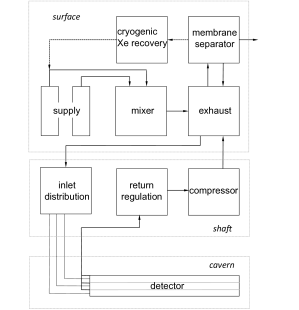
Figure 12: Schematic view of the TRD gas system. The gas circulates in a closed loop pushed by a compressor. The flow for each supermodule is determined by the pressure set at individual pressure reducers in the inlet distribution modules. The overpressure is regulated with individual pneumatic valves at the return modules. The gas is purified at the surface and, when needed, supply gas is mixed and added to the loop. For the filling and the removing of the expensive xenon, semipermeable membranes are used to separate it from the CO₂. The recovered xenon can be treated in a cryogenic plant in order to remove accumulated N₂, prior to storage.

3.3.1 Distribution

Xenon is a heavy gas; its standard condition density at ambient conditions is $5.76\text{\,}\mathrm{k}\mathrm{g}\mathrm{/}\mathrm{{}^{3}}\mathrm{m}$, 4.7 times that of air. This means that over the $7\text{\,}\mathrm{m}$ height-span of the TRD in the experiment, the total hydrostatic pressure difference between the top and the bottom supermodules would be about $2.8\text{\,}\mathrm{mbar}$. In order to overcome this, gas is circulated separately through each supermodule (except the top three and the bottom three, which are installed at similar heights) and the pressure is thus individually regulated to equal values everywhere. In addition, due to the different heights of the supermodules, the gas, supplied from the surface, would flow unevenly through the different supermodules, the lower ones being favoured over the higher ones. This second inconvenience is overcome by supplying the gas to each supermodule from the distribution area (half way down the cavern shaft) through $4\text{\,}\mathrm{mm}$ thin lines over a length of about $100\text{\,}\mathrm{m}$. The pressure drop of the circulating gas in these lines, of several tens of mbar, is much larger than the difference in hydrostatic pressure between supermodules, and therefore nearly equal flow, at equal overpressure, is assured in all supermodules.

The six layers of the supermodules are supplied from one side (A-side) with three inlet lines, each of them serving two consecutive layers. Small bypass bellows connect two consecutive layers on the opposite side. In the A-side, a manifold arrangement is used to connect the gas outlets and a common safety bubbler, pressure sensors and back-up gas. The return outlets in each supermodule are connected together into one line which returns to the pump module. The three top and three bottom supermodules are connected to one single return line each. This arrangement results into 14 independently regulated circulation loops. Each supermodule has its own two-way bubbler, which provides the ultimate safety against over- or underpressure.

3.3.2 Pump

In the distribution area, the flow through each return line is regulated by a pneumatic valve per loop driven by the pressure sensors located at the detector. In this area, the gas is kept at a pressure slightly below atmospheric pressure, and it is stored in a $0.8\text{\,}{\mathrm{m}}^{3}$ buffer container before it is compressed by two pumps which operate at a constant frequency. The compressor module drives a bypass valve in order to maintain a calculated pressure set point at its inlet. In this manner, a dual regulation concept is used to handle the 14 loops. The role of the inlet buffer is to act as a damper of possible regulation oscillations. This pressure regulation system keeps the overpressure in the supermodule stable at $0.1\text{\,}\mathrm{mbar}$ above atmospheric pressure (set point) within $0.03\text{\,}\mathrm{mbar}$.

A $0.93\text{\,}{\mathrm{m}}^{3}$ high pressure buffer at the compressor outlet is used as a storage volume. Its content varies according to the atmospheric pressure, either by providing gas to the detectors, or by receiving it from them. The overpressure in this buffer typically ranges between 0.8 and $2\text{\,}\mathrm{bar}$. Knowledge of all the system volumes allows the pressure in the buffer to be predicted for any atmospheric pressure value. Gas leaks ultimately result in a reduction of this pressure, in that case the dynamic regulation of the high pressure triggers the injection of fresh gas from the mixer until the high pressure is restored. From this buffer, the pressurised gas is circulated up to the gas building at the surface.

3.3.3 Purifier

The purifier module consists of two 3 litre cartridges each filled with a copper catalyser which is efficient in chemically removing oxygen by oxidising the copper, and mechanically removing water by absorption. Upon saturation, the PLC switches between cartridges at the pre-defined frequency, and launches an automatic regeneration cycle where CuO₂ is reduced at high temperatures with a flow of H₂ diluted in argon. As the detector is rather gas tight, the O₂ intake through leaks is moderate, and the purifier keeps it between 0 and 3 ppm. However, H₂O diffusion, probably through the aluminised Mylar foil which constitutes the drift electrode of every read-out chamber, makes it necessary to switch between purifiers about every 3.5 days, in order to keep the H₂O content below a few hundred ppm.

3.3.4 Recirculation

The surface module is used to recirculate the gas at high enough pressure to the distribution modules in the cavern shaft area. It also contains provisions for extracting gas samples for analysis, and a bypass loop to allow for the installation of containers such as a krypton source for gain calibration (see Section 10).

3.3.5 Mixer

Under normal operation and since the gas is only exhausted through leaks, gas injection into the system happens only if the pressure in the high pressure buffer falls below a dynamic threshold, as explained above. On such occasions, the mixer is activated and injects the nominal gas mixture at a rate of a few tens of $\mathrm{l}\mathrm{/}\mathrm{h}$ until the high pressure buffer is replenished. The amount of gas injected by the mixer during a given period provides a direct measurement of the leak rate.

In addition, a second set of mass flow controllers provides flows in the $\mathrm{{}^{3}}\mathrm{m}\mathrm{/}\mathrm{h}$ range and is used for filling and emptying the detector.

3.3.6 Backup system

When the gas system is in stop mode, e.g. when there is a power failure, the safety bubbler installed on each supermodule ensures that the detector pressure always remains within about $\pm$$1.3\text{\,}\mathrm{mbar}$ relative to atmospheric pressure. In order to avoid that air, i.e. oxygen, enters the detector, the external side of the bubbler is connected to a continuous flow of neutral gas, in this case N₂, that flows through the bubbler in case of a large detector underpressure. The choice of N₂ is driven by the small influence on the gas properties that this admixture has (see Fig. 11). The full TRD is served by three independent backup lines, each with connections to six supermodule bubblers, and arranged such that the flow points downwards. In this way, if the xenon mixture is exhausted through the bubblers, it falls down the back-up line, relieving its high hydrostatic pressure. A differential pressure transmitter measures the pressure difference between the detector and the backup gas.

3.3.7 Analysis

The control of the gas quality is perhaps the most demanding aspect of running detectors where both signal amplitude and drift time information are important. This control is even more crucial for the ALICE TRD, where accurate and uniform drift velocity and gain values are needed for triggers based on online tracking and particle identification. Thus, in addition to effective tightness of the system and continuous removal of O₂ and H₂O, constant monitoring of the gas composition and in particular of the N₂ is necessary. Although for a large volume system such as that of the TRD the changes in composition are obviously slow, the precision and stability requirement of the measuring instruments are quite challenging. Furthermore, constantly measuring analysers, such as O₂, H₂O and CO₂ sensors, must be installed in the gas loop, since xenon must not be exhausted. Therefore they must be free of outgassing of contaminants into the gas.

The analysis module samples the return gas from individual supermodules in a bypass mode, before it is compressed. For this, a fraction of the gas is pushed through the analysis chain by a small pump, and returned to the loop at the compressor inlet. Usually, the PLC is programmed to continuously sample one supermodule after the other, for about 10 minutes each.

An external gas chromatograph is used to periodically measure the gas composition. This device is not in the gas loop; rather, the gas is exhausted while purging and sampling a small stream for a few seconds every few hours.

3.3.8 Membranes

One system volume of xenon is injected for operation and, typically every two or three years, removed for cleaning and storage. This means that it must be possible to separate CO₂ from Xe. This separation is achieved with a set of two semipermeable membrane cartridges. Each cartridge consists of a bundle of capillary polyimide tubes through which the mixture flows. The bundle is in turn enclosed in the cartridge case. While the CO₂ permeates through the polyimide walls, most of the xenon is contained and continues to flow into the loop. The permeating gas can be circulated through the second membrane cartridge to further separate and recover most of the Xe.

During the filling, the detector is first flushed with CO₂ and then, in closed-loop circulation, the xenon is injected as the CO₂ is removed through the membranes. The reverse process is used for the recuperation of the xenon into a cryogenic plant.

3.3.9 Recuperation

N₂ inevitably builds up in the gas through small leaks and cannot be removed by the purifier cartridges. Therefore, after each long period (2–3 years) of operation, the N₂ is cryogenically separated from the Xe. A cryogenic buffer is filled with xenon after separating it from CO₂. At the same time, CO₂ is injected into the gas system in order to replace the removed gas.

The cryogenically isolated buffer is surrounded by a serpentine pipe with a regulated flow of liquid nitrogen (LN₂) in order to keep its temperature at $-170\text{\,}\mathrm{\SIUnitSymbolCelsius}$, just above the N₂ boiling point ($-195.8\text{\,}\mathrm{\SIUnitSymbolCelsius}$). At this temperature Xe (and CO₂) freezes whereas N₂ stays in the gaseous phase. Once the buffer is full, the stored gas is pumped away. After this, the buffer is heated up in a regulated way, and the evaporating Xe is compressed into normal gas cylinders. The resulting Xe has typically a N₂ contamination of <1%, and the total Xe loss (due to the efficiency of the membranes and the cryogenic recovery process) is about $1\text{\,}{\mathrm{m}}^{3}$ for a full recovery operation.

3.4 Operational challenges

The gas system has been operating reliably over several years in several modes, but mainly in so-called run mode. Aside from minor incidents, a number of important leaks have been dealt with, which deserve a brief description.

3.4.1 Viscous leaks

As part of the standard quality assurance procedure, a leak test was performed on each chamber prior to installation in the supermodule. The leak test consisted of flushing the chamber with gas and measuring the O₂ contamination at the exhaust, where the overpressure was typically about $1\text{\,}\mathrm{mbar}$. It was found, however, that a supermodule would lose gas even if the O₂ content was very low. The reason turned out to be the particular construction of the pad planes, which are glued to a reinforcement honeycomb panel with a carbon fibre sheet. Viscous leaks would develop between the glued surfaces and gas would find its way out through the cut-outs for the signal connections machined in the honeycomb sandwich. The impedance of this kind of leak is large enough that gas can escape the detector with no intake of air through back-diffusion. The concerned read-out chambers were then extracted and repaired, and the leak tests on subsequent chambers were modified such that the O₂ was measured both at over- and underpressure in the read-out chamber, resulting in a tight system.

3.4.2 Argon contamination

At one point, the routine gas analysis with the gas chromatograph showed increasing levels of Ar in the Xe-CO₂ mixture. This elusive leak came from a faulty pressure regulator which was pressurised with argon on the atmospheric side. Occasionally, depending on the pressure, the membrane of the regulator would leak and let Ar enter the gas volume. A total of 1% Ar accumulated in the mixture and was removed by cryogenic distillation, together with N₂.

3.4.3 Leak in pipe

The last major leak in the system was detected when suddenly the pressure at the high pressure buffer started to steadily decrease. Any leak of the system would appear, while running, as a decrease in the high pressure buffer, because the system always ensures the right overpressure at the read-out chambers. By stopping the system and isolating all of its modules, it was found that the source of the leak was a long, stainless steel pipe which connected the compressor module, half way down the cavern shaft, to the surface, where the gas, still at high pressure, is cleaned and recirculated. It was not possible to find the exact location of the leak. This was solved by replacing the pipe by a spare.

4 Services

The supermodules installed in the space frame require service infrastructure for their operation. To reduce the weight, the connections (low and high voltage, cooling, gas, read-out, and control lines) are routed via dedicated frames on the A- and C-side, respectively. Both frames are $2\text{\,}\mathrm{m}$ extensions of the space frame with similar geometry, but mechanically independent except for the flexible services. Most of the equipment, such as the low-voltage power supplies, is placed in the cavern underground and thus inaccessible during beam operation. Some devices are situated in counting rooms in the cavern shaft, which are supervised radiation areas but accessible.

4.1 Low voltage

The low voltage system supplies power to various components of the TRD. The largest consumer is the Front-End Electronics (FEE), i.e. the electronics of the Read-Out Boards (ROB) mounted on the chamber (see Section 5). To minimise noise, separate (floating) voltage rails are used for analogue and digital components. The power supply channels for analogue $1.8\text{\,}\mathrm{V}$, analogue $3.3\text{\,}\mathrm{V}$, and digital $1.8\text{\,}\mathrm{V}$ are grouped such that one power supply channel supplies two layers of a supermodule. For the digital $3.3\text{\,}\mathrm{V}$ there is one channel per supermodule. For each supermodule, this results in the supply channels listed in Table 3. The DCS boards (see Section 4.4) are powered by a power distribution box (PDB), two of which (in two adjacent supermodules) are supplied by a dedicated channel. The PDBs are controlled by Power Control Units (PCU) over a redundant serial interface.

Channel	$\mathbf{U_{\mathrm{nom}}(\mathrm{V})}$	$\mathbf{I_{\mathrm{typ}}(\mathrm{A})}$
3 x Analogue $1.8\text{\,}\mathrm{V}$	2.5	125
3 x Analogue $3.3\text{\,}\mathrm{V}$	4.0	107
3 x Digital $1.8\text{\,}\mathrm{V}$	2.5	95–150
Digital $3.3\text{\,}\mathrm{V}$	4.0	110
DCS boards	4.0	2 $\times$ 30

Table 3: Number of low voltage channels, nominal voltages and typical currents for the electronics on the chamber-mounted read-out boards of one supermodule. The current for the TRAP cores (digital 1.8 V) increases with the trigger rates. The current for the DCS boards is 2 $\times$ $30\text{\,}\mathrm{A}$ for two adjacent sectors.

Because of the high currents, the intrinsic resistances of the cables and connections are critical and are constantly monitored by measuring the voltage drop between the power supply unit (terminal voltage) and the patch panel at each supermodule (sense voltage). Typical values are 6–$8\text{\,}\mathrm{m\SIUnitSymbolOhm}$, depending on the cable length. In addition, the voltages at the end of each power bus bar are monitored.

The Global Tracking Unit (GTU) (see Section 5.3) uses additional power supplies which are shared with the PCUs. The pretrigger system (see Section 5.1) is powered by separate power supplies, laid out in a fail-safe redundant architecture.

Different customizations of the Wiener PL512 power supply units are used. The power supplies feeding the FEE are connected to a PLC-based interlock based on the status of the cooling. Power is automatically cut in case of a cooling failure.

During the Run 1 operation, several low-voltage connections on the supermodules showed increased resistivity resulting in excessive heat dissipation, which in some cases required to switch off part of the detector until the problem could be fixed during an access. Later, during LS 1, the affected supermodules were pulled out of the experiment and the connections were reworked in the cavern. The supermodules were re-inserted and re-commissioned immediately after the rework. The complete procedure took about one day per supermodule.

4.2 Cooling

The complexity of the cooling system, whose cooling medium is deionised water, is driven by the large amount of heat sources (more than $100\,000\text{\,}$) distributed over the complete active area of the detector. Heat is produced by the MCMs and the Voltage Regulators (VR) on the read-out boards, the DCS boards, and the power bars. The total heat dissipation in a supermodule amounts to about $3.3\text{\,}\mathrm{kW}$, of which about $2.6\text{\,}\mathrm{kW}$ are produced in the FEE, the remaining $700\text{\,}\mathrm{W}$ originate from the voltage regulators and the bus bars. The DCS boards contribute with about $130\text{\,}\mathrm{W}$ per supermodule. Overall, the rate of heat to be carried away during detector operation amounts to $55\text{\,}\mathrm{kW}$ and $70\text{\,}\mathrm{kW}$ in Pb–Pb and pp collisions, respectively, due to different read-out rates. Apart from the power bus bars, the heat sources are positioned on top of the read-out boards.

In the cooling system the pressure is kept below atmospheric pressure. Thus a leak leads to air entering in the system but no water is spilled onto the detector. The cooling plant [67] consists of a $1500\text{\,}\mathrm{l}$ storage tank positioned at the lowest point outside the solenoid magnet, which is able to contain all the water of the installation, the circulation pump, the 18 individual circuits that supply cooling water to the 6 layers of each supermodule, and the heat exchanger connected to the CERN chilled water network. The reservoir is kept at 300–$350\text{\,}\mathrm{mbar}$ below atmospheric pressure by means of a vacuum pump that also removes any air collected through small leaks. In addition, the pressure of the circulation pump ($1.8\text{\,}\mathrm{bar}$) and the diameter of all pipes are chosen such that a sub-atmospheric pressure is maintained in all places of the detector, despite a difference in height of about $7\text{\,}\mathrm{m}$ between the lowest and the highest supermodule. Each circuit is equipped with individual heaters and balancing valves in order to control the temperature and the flow in each loop separately. The heaters are regulated by a proportional-integral-derivative controller. A temperature stability in the cooling water of $\pm$$0.2\text{\,}\mathrm{\SIUnitSymbolCelsius}$ is achieved. The typical water flow is about $1300\text{\,}\mathrm{l}\mathrm{/}\mathrm{h}$ per supermodule. To avoid corrosion a fraction of the total water flow is passed by a deioniser to keep the water conductivity low. As the water is in contact with similar materials (stainless steel and aluminium), the TRD cooling system also supplies the water to the cooling panels of the thermal screening between TPC and TRD [31].

The loop regulations and cooling plant control is done by a PLC. Warnings and alarms are issued by the PLC if the parameters are outside the allowed intervals and read out by the Detector Control System (see Section 6). Two independent security levels were implemented in each loop. The first continuously monitors the pressure of each loop and stops the water circulation of the cooling plant if any value reaches atmospheric pressure. Secondly, large safety valves were installed at the entrance to each supermodule. They will open in case an overpressure of $50\text{\,}\mathrm{mbar}$ is reached, providing a low resistance path for the water evacuation in case of emergency.

The cold water is supplied in the lowest point of each supermodule and the warm water is collected on the highest point in order to have more homogeneous water flow in all pipes. A water manifold at one end-cap of the supermodule distributes the water in parallel to the 6 layers inside each supermodule, and on the opposite side a similar manifold collects the warm water. In each layer, two rectangular pipes along the $z$-direction (65 $\times$ 8 $\times$ $7500\text{\,}{\mathrm{}}^{3}\text{\,}\mathrm{mm}$) supply (collect) water to (from) the meanders, 76 individual cylindrical aluminium pipes ($3\text{\,}\mathrm{mm}$ in diameter) running across the $y$-direction where the heat sources are. A total of 17 meander types were designed for the system. To bring the water from the rectangular pipes to the individual meanders, the rectangular pipe has small stainless steel pipes ($3\text{\,}\mathrm{mm}$ diameter and $5\text{\,}\mathrm{cm}$ length) soldered at the proper position for each MCM row. A Viton tube of about $2\text{\,}\mathrm{cm}$ length is used to connect the small stainless steel pipes and the meanders as well as for the connections between the two meanders (one per ROB) in $y$-direction. A total of about 25000 Viton tube connectors were used in the system. This kind of connector was previously used in the CERES/NA45 leakless cooling system [68] because of its low price and reliability.

The cooling pad mounted on top of the heat source consists of an $0.4\text{\,}\mathrm{mm}$ thick aluminium plate. The meander is glued on top of the pad by aluminium-filled epoxy (aluminium powder: Araldite^® 130:100 by weight) to increase the thermal conductivity. In order to maximise the heat transfer, the longest possible path was chosen. The choice of aluminium was driven by the necessity of keeping the material budget as low as possible in the active area of the detector.

4.3 High voltage

The high voltage distribution for the drift field and the anode-wire plane is made separately for each chamber, reducing the affected area to one chamber in case of failure. The power supplies for the drift channels and anode-wires were purchased from ISEG [69] (variants of the model EDS 20025). Each module has 32 channels, which are grouped in independent 16-channel boards. Each channel is independently controllable in terms of the voltage setting and current limit as well as monitoring of current and voltage. Eight modules are placed into each crate and remotely controlled via CANbus (Controller Area Network) from DCS (see Section 6). The HV crates are placed in one of the counting rooms in the cavern shaft, which allows access even during beam operation.

For each of the 30 read-out chambers in a supermodule one power supply is needed for the drift field and one for the anode-wire plane. A multiwire HV cable connects the 32 channel HV module with a 30 channel HV fanout box (patch box) located at one end of the supermodule, where the output is redistributed to single wire HV cables (see Section 2.3). The individual HV cables are then connected to a HV filter box, mounted along the side of the read-out chamber. The HV filter box supplies the HV to the 6 anode segments and the drift cathode of the read-out chamber, and in addition it allows connection of the HV ground to the chamber ground. It consists of a network of a resistor and capacitors ($2.2\text{\,}\mathrm{nF}$ and $4.7\text{\,}\mathrm{nF}$) to suppress load-induced fluctuations of the voltages in the chamber.

The HV crates are equipped with an Uninterruptible Power Supply (UPS) and a battery to bridge short term power failures. In case of a longer power failure (> $10\text{\,}\mathrm{s}$) a controlled ramp-down is initiated, i.e. the HV of the individual drift and anode-wire channels is slowly ramped down. Details on maximum applied voltages, channel equalisation, ramp speed as well as high-voltage instability observed during data taking are discussed in Sections 6 and 7.3.

4.4 Slow control network

The slow control of the TRD is based on Detector Control Systemboards [70]. They communicate with the DCS (see Section 6) by a $10\text{\,}\mathrm{M}\mathrm{bit}\mathrm{/}\mathrm{s}$ Ethernet interface, mostly using Distributed Information Management (DIM) as protocol for information exchange. The use of Ethernet allows the use of standard network equipment, but a dedicated network restricted to the ALICE site is used. The DCS boards are used as end points for the DCS to interact with subsystems of the detector. Later sections will discuss how the DCS boards are used as interface to the various components, e.g. the front-end electronics or the GTU.

The DCS boards were specifically designed for the control of the detector components and are used by several detectors in ALICE. At the core, the board hosts an Altera Excalibur EPXA1 (ARMv4 core + FPGA), which hosts a Linux operating system on the processor and user logic in the FPGA fabric depending on the specific usage of the board. The DCS board also contains the Trigger and Timing Control receiver (TTCrx) for clock recovery and trigger reception. The Ethernet interface is implemented with a hardware PHY (physical layer) and a soft-Media Access Controller (MAC) in the FPGA fabric. In case of the boards mounted on the detector chambers, the FPGA also contains the Slow Control Serial Network (SCSN) master used to configure the front-end electronics. Further general purpose I/O lines are, e.g. used for JTAG and I²C communication.

Since the Ethernet connections are used for configuration and monitoring of the detector components, reliable operation is crucial. All DCS boards are connected to standard Ethernet switches installed in the experimental cavern outside of the solenoid magnet. Because of the stray magnetic field and the special Ethernet interface of the DCS board (no inductive coupling), there are limitations on the usable switches. Since the failure of an individual switch would result in the loss of connectivity to a large number of DCS boards, a custom-designed Ethernet multiplexer was installed in front of the switches in the second half of Run 1. This allows the connection of each DCS board to be remotely switched between two different switches with separate uplinks to the DCS network. The multiplexers themselves are implemented with fully redundant power supplies and control interfaces.

5 Read-out

The read-out chain transfers both raw data and condensed information for the level-1 trigger. While the former requires sufficient bandwidth to minimise dead time, the latter depends on a low latency, i.e. a short delay of the transmission. The data from the detector are processed in a highly parallelised read-out tree. Figure 13 provides an overview and relates entities of the read-out system to detector components. In the detector-mounted front-end electronics, the data are processed in Multi-Chip Modules grouped on Read-Out Boards (ROB) and eventually merged per half-chamber. Then, they are transmitted optically to the Track Matching Units (TMU) as the first stage of the Global Tracking Unit (GTU). The data from all stacks of a supermodule are combined on the SuperModule Unit (SMU) and eventually sent to the Data AcQuisition system (DAQ) through one Detector Data Link (DDL) per supermodule.

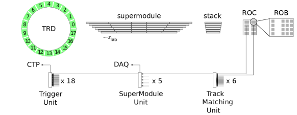
Figure 13: Detector structures and corresponding read-out stages [71]. The top row of the figure represents the detector and the bottom row the GTU components. The dimensions are not to scale.

The read-out of the detector is controlled by trigger signals distributed to both the FEE and the GTU. The ALICE trigger system is based on three hardware-level triggers (level-0, 1, 2) and a High Level Trigger (HLT) [72] implemented as a computing farm. In addition to these levels, the FEE requires a dedicated wake-up signal as described in the next subsection.

5.1 Pretrigger and LM system

Both FEE and GTU must receive clock and trigger signals, which are provided by the Central Trigger Processor (CTP) [73] using the Trigger and Timing Control (TTC) protocol over optical fibres. While the GTU only needs the level-0/1/2 and is directly connected to the CTP, the FEE requires a more complicated setup. To reduce power consumption, it remains in a sleep mode when idle and requires a fast wake-up signal before the reception of a level-0 trigger to start the processing. During Run 1, an intermediate pretrigger system was installed within the solenoid magnet [74, 75]. Besides passing on the clock and triggers received from the CTP, it generated the wake-up signal from copies of the analogue V0 and T0 signals (reproducing the level-0 condition) and distributed it to the front-end electronics. In addition, the signals from TOF were used to generate a pretrigger and level-0 trigger on cosmic rays. Because of limitations of this setup, the latencies of the contributing trigger detectors at the CTP were reduced for Run 2 (also by relocating the respective detector electronics) such that the functionality of the pretrigger system could be integrated into the CTP. The latter now issues an LM (level minus 1) trigger for the TRD before the level-0 trigger. An interface unit (LTU-T) was developed for protocol conversion [76] in order to meet the requirements of the TRD front-end electronics. A comparison of the two designs is shown in Fig. 14. The new system has been used since the beginning of collision data taking in Run 2.

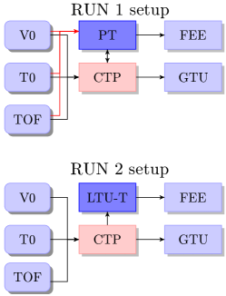
Figure 14: In Run 1, the wake-up signal required for the front-end electronics was generated by a dedicated pretrigger system. In Run 2, the functionality was implemented in the central trigger processor and the LTU-T serves as an interface to the TRD FEE.

5.2 Front-end electronics

The FEE is mounted on the back-side of the read-out chamber. It consists of MCMs which are connected to the pads of the cathode plane with flexible flat cables. An MCM comprises two ASICs, a PASA and a TRAP, which feature a large number of configuration settings to adapt to changing operating conditions. The signals from 18 pads are connected to the charge-sensitive inputs of the PASA on one MCM. An overview of the connections is shown in Fig. 15.

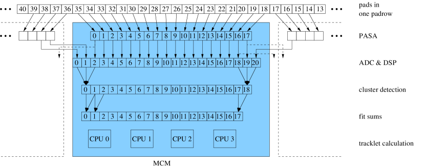
Figure 15: Connections in one MCM [66].

The very small charges induced on the read-out pads (typically $7\text{\,}\mathrm{\SIUnitSymbolMicro A}$ during $1\text{\,}\mathrm{ns}$) are not amenable to direct signal processing. Therefore, the signal is first integrated and amplified by a Charge Sensitive Amplifier (CSA). Its output is a voltage signal with an amplitude proportional to the total charge. The CSA has a relatively long decay time, which makes it vulnerable to pile-up. A differentiator stage removes the low frequency part of the pulse. The exponential decay of the CSA feedback network, in combination with the differentiator network, leads to an undershoot at the shaper output with the same time constant as the CSA feedback network. A Pole-Zero network is used to suppress the undershoot. A shaper network is required to limit the bandwidth of the output signal and avoid aliasing in the subsequent digitisation process. At the same time the overall signal-to-noise ratio must be optimised. These objectives are achieved by a semi-Gaussian shaper, implemented with two low-pass filter stages. Each stage consists of two second-order bridged-T filters connected in cascade. The second shaper consists of a fully differential amplifier with a folded cascode configuration and a common-mode feedback circuit. This circuit network was implemented to prevent the output of the fully differential amplifier from drifting to either of the two supply voltages. It establishes a stable common-mode voltage. The last stage in the chain comprises a pseudo-differential amplifier with a gain of 2. This stage adapts the DC voltage level of the PASA output to the input DC-level of the TRAP ADC [77].

Parameter	Value
PASA gain	$12\text{\,}\mathrm{m}\mathrm{V}\mathrm{/}\mathrm{f}\mathrm{C}$
PASA power	$15\text{\,}\mathrm{m}\mathrm{W}\mathrm{/}\mathrm{c}\mathrm{h}\mathrm{a}\mathrm{n}\mathrm{n}\mathrm{e}\mathrm{l}$
PASA pulse width (FWHM)	$116\text{\,}\mathrm{ns}$
PASA noise (equivalent charge)	$1000~{}\mathrm{e}$
TRAP power	$12.5\text{\,}\mathrm{m}\mathrm{W}\mathrm{/}\mathrm{c}\mathrm{h}\mathrm{a}\mathrm{n}\mathrm{n}\mathrm{e}\mathrm{l}$
TRAP ADC depth	10 bit
TRAP sampling frequency	$10\text{\,}\mathrm{MHz}$

Table 4: Achieved PASA and TRAP characteristics.

The differential PASA outputs are fed into the ADCs of the TRAP, the second ASIC on the same MCM. The PASA and TRAP parameters are listed in Table 4. The TRAP is a custom-designed digital chip produced in the UMC $0.18\text{\,}\mathrm{\SIUnitSymbolMicro m}$ process. The TRAP comprises cycling 10-bit ADCs for 21 channels, a digital filter chain, a hardware preprocessor, four two-stage pipelined CPUs with individual single-port, Hamming-protected instruction memories (IMEM, 4k x 24 bit), about 400 configuration registers usable by the hardware components, a quad-port Hamming-protected data memory (DMEM, 1k x 32 bit), and an arbitrated Hamming-protected data bank (DBANK, 256 x 32 bit) [78]. Three excess ADC channels are fed with the amplified analogue signal from the two adjacent MCMs to avoid tracking inefficiencies at the MCM boundaries. The signals of all 21 channels are sampled and processed in time bins of $100\text{\,}\mathrm{ns}$. The number of time bins to be read out, can be configured in the FEE. At the beginning of Run 1 24 time bins were conservatively read out. At a later stage the number of time bins was reduced to 22 in order to reduce the readout time and the data volume.

The first step in the TRAP is the digitisation of the incoming analogue signals. In order to avoid rounding effects, the ADC outputs are extended by two binary digits and fed into the digital filter chain. First, the pedestal of the signal is equilibrated to a configurable value. Then, a gain filter is used to correct for local variations of the gain, arising either from detector imperfections or the electronics themselves. A tail cancellation filter can be used to suppress the ion tails. The filtered data are fed into a pre-processor which contains hardware units for the cluster finding. The four CPUs (MIMD architecture) are used for the further processing. The local tracking procedure is discussed in detail in Section 12.1.

The MCMs are mounted on the ROB. On each board, 16 chips are used to sample and process the detector signals. A full detector chamber is covered by 8 ROBs (6 for chambers in stack 2). The read-out is organised in a multi-level tree. First, the data from four chips are collected by so-called column merger chips. The latter, in addition to processing the data from their own inputs, receive the data from three more MCMs. The data are merged and forwarded to the board merger, which combines the data from all chips of one ROB. One ROB per half-chamber carries an additional MCM which acts as half-chamber merger (without processing data of its own). It forwards the data to the Optical Read-out Interface (ORI) from where it is transmitted through an optical link (DDL) to the GTU. The link is operated at 2.5 Gbit/s and is implemented for uni-directional transmission without handshaking, i.e. the receiving side must be able to handle the incoming data for a complete event as it arrives. As the FEE does not provide multi-event buffering, the detector is busy until the transmission from the FEE is finished. The slowest half-chamber determines the contribution to the dead time of the full detector.

5.3 Global Tracking Unit

The GTU receives data via 1044 links from the FEE. The aggregate net bandwidth amounts to $261\text{\,}\mathrm{G}\mathrm{B}\mathrm{/}\mathrm{s}$. The two main tasks of the GTU are the calculation of level-1 trigger contributions from a large number of track properties in about $2\text{\,}\mathrm{\SIUnitSymbolMicro s}$ and the preparation of the event data for read-out. Accordingly, the data processing on the GTU features a trigger path, which is optimised for low latency, and a data path, which equips the detector with the capability to buffer up to 4 events (multi-event buffering, MEB). The derandomisation of the incoming data rate fluctuations with multiple event buffers minimises the read-out related dead time. The data transfer from the GTU to the DAQ contributes to the dead time only when the read-out rate approaches the rate which saturates the output bandwidth as shown in Fig. 16.

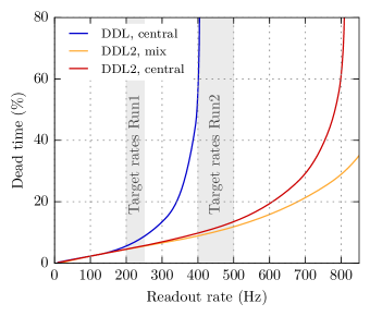
Figure 16: Simulation of the dead time as function of the read-out rate in Pb–Pb collisions for the effective DDL bandwidth in Run 1 (DDL) and Run 2 (DDL2). The simulation assumes a 5% L1/L0 accept ratio and no L2 rejects. The scenarios central and mix correspond to an event size of 470 kB and 310 kB per supermodule, respectively, mimicking thus different event multiplicities.

The GTU consists of three types of FPGA-based processing nodes organised in a three-layer hierarchy (see Fig. 17). The central component of all nodes is a Virtex-4^© FX100 FPGA, supplemented by a $4\text{\,}\mathrm{MB}$ source-synchronous DDR-SRAM, $64\text{\,}\mathrm{MB}$ DDR2-SDRAM and optical transceivers. Depending on the type, the nodes are equipped with different optical parts and supplementary modules. 90 TMUs and 18 SMUs are organised in 18 segments of 5+1 nodes (corresponding to the 18 sectors). The TMUs and SMU of a segment are interconnected using a custom LVDS backplane, which is optimised for high-bandwidth transmissions at low latency. A single top-level Trigger Unit (TGU) is connected to the SMUs of the individual segments via LVDS transmission lines.

Figure 17: Major design blocks of the TMU and SMU stages of the GTU and data flow. The busy and trigger logic information are combined on the TGU before transmission to the CTP.

The data from one stack is received by the corresponding TMU. Each TMU implements the global online tracking, which combines pre-processed track segments to tracks traversing the corresponding detector stack, as first stage of the trigger processing (see Section 12). The TMUs furthermore implement the initial handling and buffering of incoming events as a pipelined data push architecture. Input shaper units monitor the structural integrity of the incoming data and potentially restore it to a form that allows for stable operation of all downstream entities. Dual-port, dual-clock BRAMs in the FPGA are utilised to compactify data of the 12 incoming link data streams to dense, wide lines suitable for storage in the SRAM. The SRAM provides buffer space for multiple events and its controller implements the required write-over-read prioritisation to ensure that data can be handled at full receiver bandwidth. On the read side, a convenient interface is provided to read out or discard stored events in accordance to the control signals generated by the segment control on the SMU.

Via its DCS board the SMU receives relayed trigger data issued by the CTP to synchronise the operation of the experiment. The trigger sequences are decoded, and converted to suitable control signals and time frames to steer the operation of the segment. The segment control on the SMU supports operation with multiple, interlaced trigger sequences in order to support the concurrent handling and buffering of multiple events. Upon reception of a level-2 trigger, the SMU requests the corresponding event data from the event buffers and initiates the building of the event fragment for read-out. The built fragment contains, in addition to the data originating from the detector, intermediate and final results from tracking and triggering relevant for offline verification, as well as checksums to quickly assess its integrity. The SMU implements the read-out interface to the DAQ/HLT with one DDL. The endpoint of the DDL is a Source Interface Unit (SIU), which in Run 1 was a dedicated add-on card mounted on the SMU backside that operates at a line rate of $2.125\text{\,}\mathrm{G}\mathrm{bit}\mathrm{/}\mathrm{s}$. The read-out upgrade for Run 2 integrates the functionality of the SIU into the SMU FPGA and employs a previously unused transceiver on the SMU at a line rate of $4\text{\,}\mathrm{G}\mathrm{bit}\mathrm{/}\mathrm{s}$. The elimination of the interface between SMU and SIU add-on card, the higher line rate as well as data path optimisations resulted in an increase of the effective DDL output bandwidth from $189\text{\,}\mathrm{M}\mathrm{B}\mathrm{/}\mathrm{s}$ to $370\text{\,}\mathrm{M}\mathrm{B}\mathrm{/}\mathrm{s}$ in Run 2. Figure 16 illustrates the performance improvement for the assumed data taking scenarios. With the upgrade the read-out-related dead time can be kept at an acceptable level. The almost linear increase at low rates is due to the dead time associated with the L0–L1 interval and the FEE-GTU transmission. The typical aggregate output bandwidth for all 18 supermodules is $126\text{\,}\mathrm{M}\mathrm{B}\mathrm{/}\mathrm{s}$, $202\text{\,}\mathrm{M}\mathrm{B}\mathrm{/}\mathrm{s}$, and $1260\text{\,}\mathrm{M}\mathrm{B}\mathrm{/}\mathrm{s}$ in pp, p–Pb, and Pb–Pb collisions (see also Section 7.3).

The top-level TGU consolidates the status of the segments, which operate independently in terms of read-out, as well as the segment-level contributions of the triggers. It constitutes the interface to the CTP, to which it communicates the detector busy status and the TRD-global trigger contributes for various signatures (see Section 12).

6 Detector Control System

The purpose of the DCS is to ensure safe detector conditions, to allow fail-safe, reliable and consistent monitoring and control of the detector, and to provide calibration data for offline reconstruction. In addition it provides detailed information on subsystem conditions and full functionality for expert monitoring and detector operation. Tools were implemented to reduce the operational complexity and the information on detector conditions to a level that allows operators to monitor and handle the detector in an intuitive and safe way. The TRD DCS is integrated with the rest of the ALICE detector control systems into one system which is operated by one operator.

6.1 Architecture

Figure 18: Overview of the DCS software architecture. The tree structure consists of device units (boxes) and logical control units (ellipses). The abbreviations PT, DR and AN correspond to the pretrigger, the drift and anode channels, respectively.

The hardware architecture of the DCS can be divided into three functional layers. The field layer contains the actual hardware to be controlled (power supplies, FEE, etc). The control layer consists of devices which collect and process information from the field layer and make it available to the supervisory layer. Finally, the devices of the control layer receive and process commands from the supervisory layer and distribute them to the field layer.

The software on the supervisory layer is distributed over 11 server computers. It is based on the commercial Supervisory Control and Data Acquisition (SCADA) system PVSS II from the company ETM [79], now called Symatic WinCC [80]. The implementation uses the CERN JCOP control framework [81], shared by all major LHC experiments. This framework provides high flexibility and allows for easy integration of separately developed components in combination with dedicated software developed for the TRD, including Linux-based processes.

The software architecture is a tree structure that represents (sub-)systems of the detector and its devices, as shown in Fig. 18. The entities at the bottom of the hierarchy represent the devices (device units), logical entities are represented by control units. The DCS system monitors and controls 89 low voltage (LV) power supplies with more than 200 channels, and 1044 high voltage channels. The system also monitors the electronics configuration of more than one million read-out channels, the GTU, and the cooling and gas systems.

6.2 Detector safety

To ensure the safety of the equipment, nominal operating conditions are maintained by a hierarchical structure of alerts and interlocks. Whenever applicable, internal mechanisms of devices (e.g. power supply trip) are used to guarantee the highest level of reliability and security. Thresholds and status of the interlocks are controlled by the system, but the functioning of the device is independent of the communication between hardware and software. The possible range of applied settings (e.g. anode channel high voltage) is limited to a nominal range to prevent potential damage due to operator errors.

In addition, the system employs a three-level alert system, which is used to warn operators and detector experts of any unusual detector condition.

On the control and supervisory layer, cross system interlocks protect the devices and ensure consistent detector operation. These are a few examples:

• In case of a failure of the cooling plant for the FEE, a PLC-based interlock disables the LV power supplies.

• The temperature of the FEE is monitored at the control and supervisory level and interlocked with the PCU to switch off the devices in case of overheating or loss of communication to the SCADA system.

• In case of a single LV channel trip, the corresponding FEE channels are consistently switched off.

• Unstable LHC beam conditions, e.g. during injection or adjustment of the beam optics, pose a potential danger to gas-filled detectors. Therefore the HV settings are adapted to the LHC status (see Section 7.2). At injection, the anode voltages are decreased automatically to an intermediate level to reduce the chamber gain. Restoring the nominal gain is inhibited until the LHC operators declare stable beams via a data interchange protocol.

6.3 High voltage

The HV system comprises 36 HV modules in 5 crates. The 1044 HV channels, 1 of each polarity providing anode and drift voltage to each chamber, are controlled via a 250 kbit/s CAN bus through a dedicated Linux-based DIM server [82]. The published DIM services, commands and remote procedure calls (RPC) resemble the logical structure of items used in commercial process control servers: the command to change a setting is confirmed by the server via a read back setting. In addition, the actual measured value from the device is published. Update rates for different services can be adjusted independently.

The HV gain and drift velocity are equilibrated for each chamber individually to compensate for small differences in the chamber geometry. Changes of environmental conditions (atmospheric pressure and temperature) as well as small variations of the gas composition cause changes in gas gain and drift velocity. To ensure stable conditions for the level-1 trigger (see Section 12), these dynamic variations are compensated by automatic adjustments of the anode and drift voltages which are performed in between runs. These and other automatic actions on the HV are described in Section 7.2.

6.4 Detector operation

The DCS employs a dedicated Graphical User Interface (GUI) and a Finite State Machine (FSM). The FSM allows experts and operators intuitive monitoring and operation of the detector. The FSM hierarchy reflects the structure of subsystems and devices shown in Fig. 18. Detector conditions are mapped to FSM states, and these are propagated from the device level upwards to the FSM top node. Standard operational procedures (configuration of read-out and trigger electronics, ramping voltages etc.) are carried out via FSM commands which propagate down to the devices and cause a transition to a different state.

The GUI for detailed monitoring and expert operation comprises a dedicated panel for each node in the FSM tree. An example is shown in Fig. 19. Detector subsystem ‘ownership’, i.e. the right to execute FSM commands and change the detector state, is only granted to a single operator at a time, and is represented by symbolic ‘locks’. Operators can work on-site or access the DCS system remotely through appropriate gateways.

Figure 19: Graphical User Interface: example panel (FSM top node) representing the status in the year 2010 (i.e. with 10 installed TRD sectors). The FSM state of the main systems of each sector is represented by the corresponding colour; run status and alarm summary are displayed. The panel gives quick access to emergency actions and detailed monitoring panels via single mouse clicks.

The monitoring data acquired by the DCS system are stored in dedicated databases. Dedicated trending GUIs allow the experts to visualise the time dependence of the detector conditions. During data taking, the monitoring data needed for detector calibration is queried and made available for offline analysis (see Section 7.3).

7 Operation

In this section, first the commissioning steps for the detector and the required infrastructure and then the operation and performance for different collision systems are described.

7.1 Commissioning

The service connections in the cavern were prepared and tested in parallel to the construction of the supermodules. The low-voltage connections were tested with dummy loads and the leak tightness of the cooling loops was verified. The Ethernet connections were checked using both cable testers and stand-alone DCS boards. The optical fibres for the read-out were controlled for connectivity and mapping. These tests were crucial in order to identify connection problems prior to the detector installation when all connections were still well accessible.

The supermodules were installed in different installation blocks as described in Section 2. Prior to the installation the supermodules were tested at the surface site. They were rotated along the $z_{\rm lab}$-axis to the orientation corresponding to their foreseen installation position (e.g. relevant for cooling). A test setup provided all relevant services (low/high voltage, cooling, Ethernet, read-out, …) to allow a full system test of each supermodule. The testing procedure included basic functionality tests, such as water and gas tightness, front-end electronic stress tests, read-out tests as well as checks of the noise level [66].

After successful surface testing, the supermodules were installed into the space frame in the cavern (see Section 2.3). Subsequently, the services were connected and the basic tests described above repeated to verify operation in the final setup. At this stage, also the full read-out of the detector with the experiment-wide trigger and data acquisition systems was commissioned. To check the data integrity of the read-out chain, test pattern data, generated either in the FEE or in the GTU, were used. Errors observed during those tests, e.g. bitflips on individual connections on a read-out board, were cured by switching to spare lines or by masking channels from the read-out if a correction was not possible. After establishing the read-out, pedestal runs (without zero suppression) were recorded to determine the baseline and noise of each channel. If needed, further data were recorded to perform a Fourier analysis in order to identify and fix noise sources, e.g. caused by missing ground connections. In addition, these runs were used to identify inactive channels which cannot be read out.

After each installation block of new supermodules, a dedicated calibration run was performed before the actual data taking. The detector is read out with radioactive ^83mKr distributed through the gas system (see Section 10.2). Since this was usually the first high-rate data taking after the end-of-year shutdown (and installation), these runs and the preparations for them were an important step to get ready for the real data taking.

Before each physics production run, periods of cosmic-ray data taking were scheduled to study the performance of the detector system, to align individual detector components (see Section 9.1) and to provide reference spectra for particle identification (see Section 11). Data were obtained with and without magnetic field. A two-level trigger condition was used to ensure sufficient statistics in the detector acceptance, even when only the first supermodules were installed in the horizontal plane (see Section 12.3).

7.2 High voltage operation

To avoid HV trips during the critical phases of beam injection (e.g. a possible kicker failure), the anode voltages are reduced to values with very low gain. After the injection is completed, the anode voltages are ramped up from ${\sim}$$1030\text{\,}\mathrm{V}$ (gain of about a factor ${\sim}100$ lower than nominal) to an intermediate voltage of ${\sim}$$1230\text{\,}\mathrm{V}$ (gain ${\sim}6.5\%$ of nominal). The ramp speed is $6\text{\,}\mathrm{V}\mathrm{/}\mathrm{s}$. After the declaration of stable beams, the anode voltages are ramped to the nominal voltages ($U_{\mathrm{anode}}\simeq$$1520\text{\,}\mathrm{V}$) for data taking. The drift voltages always remain at nominal settings.

To equalise the gain and drift velocity of all chambers, the results from the calibration (see Section 10) are used. The nominal voltages and r.m.s. variations for drift and anode voltages are 2150$\pm$$22\text{\,}\mathrm{V}$ and 1520$\pm$$14\text{\,}\mathrm{V}$, respectively.

Based on measurements in pp, p–Pb and Pb–Pb collisions in Run 1, it has been estimated that the chambers had a time averaged current of about 200 nA. This led to a total accumulated charge of less than $0.2\text{\,}\mathrm{mC}$ per $\mathrm{cm}$ of wire for Run 1. As the chambers were validated for charges above $10\text{\,}\mathrm{m}\mathrm{C}\mathrm{/}\mathrm{c}\mathrm{m}$, it is expected that no ageing effect occurs during the time the TRD is going to be operated. Up to now, in fact no deterioration in the performance of tracking, track matching and energy resolution was observed.

The average anode current as a function of the interaction rate as measured by the T0 detectors used for the ALICE luminosity measurement has a linear dependence with a slope of $1\text{/}200\text{\,}\mathrm{n}\mathrm{A}\mathrm{/}\mathrm{H}\mathrm{z}$ for p–Pb collisions at $\sqrt{s_{\mathrm{NN}}}$ = 5.02 TeV. The slope parameter was obtained from different LHC fills ranging from minimum-bias data taking up to high rate interaction running, where the LHC background conditions can be different. Under the vacuum conditions in Run 1, about 1/3 of the current was due to the background rate, which is nearly negligible in Run 2.

The expected dependence of the measured current on detector occupancy was found. The probability for pile-up events in, e.g. p–Pb collisions at $\sqrt{s_{\mathrm{NN}}}$ = 5.02 TeV at $200\text{\,}\mathrm{kHz}$ interaction rate is about 14% when averaged over time, with a maximum of ${\sim}$24% as calculated from the bunch spacing and the number of bunch crossings in the LHC filling scheme [2, 83] as well as the integration time of the read-out chamber (drift length/drift velocity).

For the level-1 trigger it is crucial to reduce the time dependence of the drift velocity and the gain to a minimum. The former impacts the track matching, the latter the electron identification. To ensure the required stability, the anode and drift voltages are adjusted to compensate for pressure changes (the temperature is sufficiently stable). The parameters for the correction were obtained by correlating the calibration constants with pressure (see Section 10). A relative pressure change d$p/p$ results in a change of gain of d$G/G=-6.76\pm 0.04$ and drift velocity of d$v_{\mathrm{d}}$/$v_{\mathrm{d}}$ = $-1.41\pm 0.01$ [84]. In addition, the dependences of the gain and drift velocity on the anode and drift voltage, respectively, as obtained from test beam measurements [85] were used (from Run 2 onwards the dependence of gain on voltage was taken from the krypton calibration runs). This results in voltage changes of about $0.83\text{\,}\mathrm{V}$ and $1.4\text{\,}\mathrm{V}$ for a pressure change of $1\text{\,}\mathrm{mbar}$. During Run 1 the gain and the drift velocity could be kept constant within about 2.5% and 1%, respectively. These values include the precision of the determination of the calibration constants (see Section 10). The variations can be further reduced by measuring and correcting for the gas composition using a gas chromatograph installed during LS 1.

During Run 1, 10% of the anode and 5.5% of the drift channels turned out to be problematic (see Fig. 35). The respective channels had to either be reduced in anode voltage or switched off. As the detector is segmented into 5 stacks along the beam direction and 6 layers in radial direction, the loss of a single chamber in a stack is tolerable and excellent performance is still achieved for tracking and particle identification (see Sections 8 and 11). Most of the problematic chambers showed strange current behaviours (trending vs time). The de-installation of a supermodule and disassembly of the individual read-out chambers followed by detailed tests revealed that the inspected problematic anode and drift channels had broken filter capacitors ($4.7\text{\,}\mathrm{nF}$/$3\text{\,}\mathrm{kV}$). Thus, the $4.7\text{\,}\mathrm{nF}$ capacitors (see Section 4.3) were removed from the resistor chain in the last supermodules built and installed during the LS 1 (5 supermodules).

7.3 In-beam performance

After commissioning with cosmic-ray tracks and krypton calibration runs in 2009, the detector went into operation and worked reliably during the first collisions at the LHC on December 6^th 2009. Since then, the detector has participated in data taking for all collision systems and energies provided by the LHC [2]:

• pp collisions from $\sqrt{s}$ = 0.9 to 13 TeV at low interaction rates (minimum-bias data taking) and high intensities (minimum-bias data taking and rare triggering) with a maximum interaction rate of 200–$500\text{\,}\mathrm{kHz}$. During the rare trigger periods, the detector contributed level-1 triggers on high-$p_{\mathrm{T}}$ electrons and jets (see Section 12).

• p–Pb collisions at $\sqrt{s_{\mathrm{NN}}}$ = 5.02 TeV and 8 TeV with interaction rates at the level of $10\text{\,}\mathrm{kHz}$ (minimum-bias data taking) and at maximum $200\text{\,}\mathrm{kHz}$ (rare triggering). The detector contributed the same triggers as in the pp running scenario.

• Pb–Pb collisions at $\sqrt{s_{\mathrm{NN}}}$ = 2.76 TeV and 5.02 TeV with maximum interaction rates of up to $8\text{\,}\mathrm{kHz}$ (minimum-bias and rare triggering).

At the beginning of a fill, once all detectors within ALICE are ready for data taking, a global physics run is started. A run is defined in ALICE as an uninterrupted period of data taking, during which the conditions (trigger setup, participating detectors, etc.) do not change. A run can last from a few minutes to several hours until either the experimental setup or conditions have to be changed or the beam is dumped. An additional end-of-run (EOR) reason is given by the occurrence of a problem related to a given detector or system. The detector parameters measured during a run, such as the voltages and currents of the anode and drift channels as well as temperatures of the FEE, are dumped at the EOR to the Offline Conditions Database (OCDB) via the Shuttle framework [86, 87]. The relevant parameters can then be used in the offline reconstruction and analysis.

In order to ensure sufficiently stable conditions during a run, any change, such as the failure of a part of the detector, e.g. due to a LV/HV trip, triggers the ending of the run. In order to avoid too frequent interruptions, the failure of a single chamber within a stack is ignored. Technically, this is realised using the so-called Majority Unit within DCS.

All subcomponents of the TRD detector (infrastructure and gas system) are monitored via DCS (see Section 6). In case any entity deviates from nominal running conditions by pre-defined thresholds a warning is issued. The single entity is either recovered by the DCS operator in the ALICE Run Control Centre or by an expert intervention. During Run 1 data taking, most interventions were related to the recovery of single event upsets (SEU) and HV trips of problematic channels by re-configuration of the FEE or ramping up of the anode/drift channels. For Run 2 an automatic recovery of the FEE and HV was put in place.

7.3.1 Read-out performance

The event size depends on the charged-particle multiplicity. It is therefore influenced by the collision system and the background conditions of the LHC. The event size vs. charged-particle multiplicity is shown for various collision systems for one supermodule in Fig. 20. For the most central Pb–Pb collisions an event size of 800 kB per supermodule is found.

The dead time per event is composed of the front-end processing and transmission time to the GTU and a potential contribution from the shipping to DAQ. On average the former scales approximately linearly with the event size and rate, the latter is suppressed by the MEB as long as the read-out data rate stays sufficiently below the effective link bandwidth. The typical event sizes of $7\text{\,}\mathrm{kB}$, $14\text{\,}\mathrm{kB}$, $200\text{\,}\mathrm{kB}$ in minimum-bias data taking for pp, p–Pb, and Pb–Pb collisions result in front-end contributions of $20\text{\,}\mathrm{\SIUnitSymbolMicro s}$, $25\text{\,}\mathrm{\SIUnitSymbolMicro s}$, $50\text{\,}\mathrm{\SIUnitSymbolMicro s}$, respectively. This does not include the read-out induced part. However, as illustrated by the Pb–Pb case shown in Fig. 16, the detector is typically operated in the linear range of the curve, indicating that input rate fluctuations are absorbed by the MEB and that the read-out does not contribute significantly to the dead time.

The read-out rate during Run 1 and until now in Run 2 ranged from about $100\text{\,}\mathrm{Hz}$ in rare trigger periods to about $850\text{\,}\mathrm{Hz}$ in minimum-bias data taking in pp and p–Pb collisions. In Pb–Pb collisions, the read-out rate was about $100\text{\,}\mathrm{Hz}$ and $350\text{\,}\mathrm{Hz}$ for minimum-bias data taking in Pb–Pb collisions in Run 1 and up to now in Run 2, respectively.

Figure 20: Event size vs charged-particle multiplicity for various collision systems for one supermodule. To obtain the charged-particle multiplicity, global tracks (see Section 8) fulfilling minimum tracking quality criteria were counted on an event-by-event basis.

7.3.2 Radiation effects

The radiation on the TRD was for Run 1 and Run 2 (until the end of 2016) rather low both in terms of flux and dose. The following radiation calculations for the inner radius of the TRD are based on simulations obtained using the FLUKA transport code [88] and taking into account the measured multiplicities of Pb–Pb, p–Pb and pp collisions [89, 90, 91, 92, 93, 94] as well as the running scenarios (luminosities, running time, and interaction rate). For the indicated time range the Total Ionisation Dose (TID) and the Non-Ionising Energy Loss (NIEL), quoted in 1-MeV-neq fluence, were $7\cdot 10^{-3}$ krad and $2\cdot 10^{9}\rm{cm^{-2}}$, respectively. The flux of hadrons is highest in Pb–Pb collisions, because it is proportional to the product of the interaction rate and the particle multiplicity. For Pb–Pb collisions at $\sqrt{s_{\mathrm{NN}}}$ = 5.02 TeV, the flux of hadrons with $>20$ keV energy and charged particles is about $3.8\cdot 10^{-2}\rm{kHz/cm^{2}}$ and $2.5\cdot 10^{-2}\rm{kHz/cm^{2}}$, respectively. The radiation load in terms of flux and dose are far below the values, for which the experiment was designed for [1].

In the radiation environment described above, very few SEUs are observed in the electronics. The most affected device is the DCS board, for which SEUs result in occasional reboots (a few DCS boards per LHC fill). The DCS board is needed for control and monitoring but is not part of the read-out chain meaning that the reboots do not affect the data taking. The external RAM on the DCS board can be monitored for SEUs by writing and verifying known patterns in unused areas of the $\sim$13 MB memory per chamber. During 2.5 months of pp data taking at LHC luminosities of about $5\cdot 10^{30}\rm{cm^{-2}s^{-1}}$, 20 SEUs as shown in Fig. 21 were observed in the external RAM, i.e. a negligible amount compared to the occasional reboots of a few DCS boards.

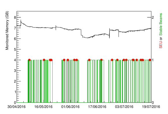
Figure 21: Monitored external DCS memory and occurrences of SEUs as a function of time. The periods of stable beam are indicated as well.

The memories of the TRAPs are Hamming-protected and, thus, resilient to SEUs. However, the configuration registers are not protected and can be affected by radiation. Therefore, the configuration is compressed and written to a Hamming-protected memory area. In this way, the registers can be checked (and corrected) against the compressed configuration.

7.3.3 Data quality assurance

The Data Quality Monitoring framework (DQM) provides online feedback on the data and allows problems to be quickly spotted and identified during data taking. The Automatic MOnitoRing Environment (AMORE) was developed for ALICE [95] and allows run-based, detector-specific analyses on the raw data. The results are visualised in a dedicated user interface. The monitored observables, such as noise level, event size per supermodule, trigger timing, FEE not sending data, are compared with reference values or diagrams (depending on the data taking scenario). Deviations from the references indicate a problem to the operator. Based on the information obtained from the online DQM all runs are directly marked with a quality flag, both globally and for the individual ALICE subdetectors. For the offline physics analyses, lists of runs are selected based on these flags according to the physics case under study.

7.3.4 Pretrigger performance

A dedicated wake-up signal is required for the FEE (see Section 5.1). It should reflect the level-0 trigger condition as closely as possible. However, as it needs to be generated before the actual level-0 trigger, it cannot use the same information. This introduces some inefficiency into the TRD read-out. In the early Run 1 LHC filling schemes (e.g. during the LHC ramp-up in 2009) with only a few colliding bunches per orbit, it was possible to send a wake-up signal for all of the bunch crossings with potential interactions. This resulted in a fully efficient operation [71]. During this time, the pretrigger system was commissioned to use the V0 and T0 signals as inputs. They could then also be used for filling schemes with many bunches. The trigger condition was configured as closely as possible to the ALICE level-0 interaction trigger, i.e. a coincidence of either the V0 or the T0 detectors (simultaneous signals in the A- and C-side, see Section 2). The efficiency of the V0- and T0-derived wake-up signals depends on the discrimination thresholds used for those detectors and on the inherent dead time between pretrigger and the abort or end of the read-out (see Section 5). The latter is particularly important when subsequent collisions are close in time, e.g. in LHC filling schemes that have bunch trains with 25 or 50 ns bunch spacing [96]. For runs taken at low interaction rates the pretrigger efficiency is above 97%; for higher rates the efficiency depends on the colliding bunch structure of the filling scheme and reaches average values down to about 83% in Run 1 [71]. These inefficiencies were avoided with the LM system used in Run 2 (see Section 5.1).

The analysis of electrons from heavy-flavour hadron decays in p–Pb collisions at $\sqrt{s_{\mathrm{NN}}}$ = 5.02 TeV in events satisfying the pretrigger condition showed no bias compared to results from events triggered with the ALICE level-0 minimum-bias interaction trigger [97].

8 Tracking

The charged particle tracking in the ALICE central barrel is based on a Kalman filtering [98]. Track finding and fitting are performed simultaneously [2]. The algorithm operates on clusters of track hits from the individual detectors. The clusters carry position information and, depending on the detector, the amount of charge from the ionisation signal. The cluster parameters are calculated locally from the raw data, implying that the cluster finding can be parallelised.

The global tracking starts from seed clusters at the outer radius of the TPC (see Fig. 1). During the first inward propagation of the tracks previously unassigned TPC clusters are attached while updating the track parameterisation at the same time. If possible, the track is further propagated to the ITS. Subsequently, an outward propagation adds information from TRD, TOF, and HMPID. A second inward propagation is used to obtain the final track parameters, which are stored at a few important detector positions, most importantly at the primary vertex.

The TRD contributes to the tracking in various ways. First, it adds roughly $70\text{\,}\mathrm{cm}$ to the lever arm, which improves significantly the momentum resolution for high-$p_{\mathrm{T}}$ tracks. Second, it increases the precision and efficiency of assigning clusters from the detectors at larger radii, in particular the TOF, to propagated tracks. In addition, the TRD is used as reference to obtain correction maps for distortions in the TPC, which arise from the build up of space charge at high interaction rates. For this the TRD and ITS track segments are reconstructed using as seeds the TPC tracks (with relaxed tolerances accounting for potential distortions). Then, the estimate of the real track position is built as a weighted average of the ITS and TRD refitted tracks (without TPC information). The TPC distortions are deconvoluted from the residuals between these interpolations and the measured TPC cluster positions.

The tracking in the TRD can be subdivided into the formation of tracklets (track segments within one read-out chamber) from clusters and the updating of the global tracks based on the tracklets. These steps are performed layer-by-layer. The chambers within a layer can be treated in parallel. For each layer, a seed track is prepared by propagation from the TPC and used to calculate the intersection with a chamber. Based on this information a tracklet is formed from the clusters in the vicinity of this intersection and then the track parameterisation is updated accordingly. In the following, details of the individual steps will be given.

8.1 Clusterisation

Primary ionisation in the detector gas leads to a signal that spreads over several pads. Because of the slower ion drift, the charge carries over into subsequent time bins, resulting in a correlation between time bins (see Section 2.1). The cluster algorithm combines the data from adjacent pads in the same time bin, producing clusters with information on position and total charge. The former is calculated from the weighted mean of the charge shared between adjacent pads (up to 3). Look-Up Tables (LUT) are used to relate the measured charge distribution to the actual position. These LUTs are the result of calculations for the different pad width sizes, based on measurements in a test beam [46]. The cluster position can deviate from the LUT values because of detector parameters which are subject to calibration (see Section 10), most importantly the drift velocity $v_{\mathrm{d}}$ and the time offset $t_{0}$ (time corresponding to the position of the anode wires, see Fig. 30). In addition, a correction for the $E\times B$ effect is applied. The complete position characterisation also includes the estimated uncertainty, which determines the weight for updating the global track. The uncertainties are derived from differential analyses of Monte Carlo simulations. Cluster properties such as the deposited energy, time bin, and reconstructed position relative to the pad with the maximum charge are taken into account as well as particle level characteristics such as electrical charge and incident angle. A linear model relates all uncertainties with parameters being defined by all conditions determining a cluster.

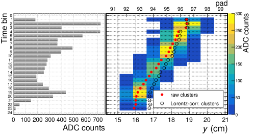
Figure 22: Signal produced by a positively charged particle ($p_{\mathrm{T}}=0.5~{}\mathrm{GeV}\!/c$). Left: Total charge per time bin used for particle identification. Right: Ionisation signal vs. pad number and time bin. The cluster positions are shown as reconstructed from the charge distribution (raw clusters) and after correction for the $E\times B$ effect (Lorentz-corr. clusters).

8.2 Track reconstruction

For the preparation of the TPC-based track seed used to match with the TRD clusters, the Kalman parameterisation (at the outer radius of the TPC) is propagated to the radial position of the anode wires of a given chamber. At this radius the position is least affected by variations in calibration parameters. If a chamber is rotated with respect to the tracking frame, the radial position of the anode wires depends on the intersection point of the track in the $y$-$z$ plane. As this is only known after the propagation, the preparation of the track seed is an iterative process.

The clusters that are assigned to the seed track in a given layer are combined into tracklets. A straight line fit is sufficient for their description since the negligible sagitta of the trajectory is only of the order of tens of microns.

Since in the read-out chamber the electrons drift in the radial direction, that is approximately parallel to the track, and due to the long ion tails, the signals pile up. The measured charges, sampled in time intervals of $100\text{\,}\mathrm{ns}$, are therefore correlated between different time samples. Since such correlations degrade the angular resolution, a tail cancellation correction is applied [46]. It subtracts an exponential tail proportional to the current signal from the subsequent samples for each read-out pad.

The number of pads on the the read-out plane onto which a track is projected depends on the track incident angle. For decreasing transverse momentum, more pads will carry a signal. The Lorentz angle also affects this spread. For negatively (positively) charged particles the Lorentz drift is along (opposite to) the track inclination, independent of the polarity of the magnetic field. On average, negatively charged particles are thus spread over fewer pads than positively charged ones. In the right panel of Fig. 22, an example of a positively charged particle of $p_{\mathrm{T}}=0.5~{}\mathrm{GeV}\!/c$ (worst case) is shown. Its projection spans over 6 pads.

The procedure to find candidates for seeds involves a preliminary stage in which clusters are searched in the neighbourhood of the propagated seed. In Fig. 23 the mean and width of the residuals are shown for the arising tracklets in $\Delta y$ in layer 0 as a function of the seed $p_{\mathrm{T}}$. The imperfect tail cancellation results in different position biases for tracklets from positive and negative tracklets, the signal spreading over more pads for the former.

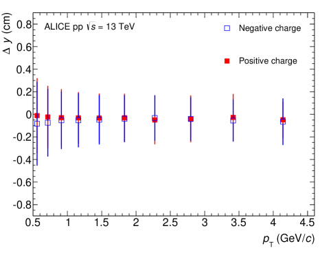
Figure 23: Residuals in $\Delta y$ of tracklets with respect to global tracks as a function of $p_{\mathrm{T}}$ in pp collisions at $\sqrt{s}=13~{}\mathrm{TeV}$. For every bin the mean (marker) and r.m.s. width (error bar) of the distribution are shown.

8.3 Performance

The relative frequencies of the number of tracklets assigned to a track are shown in Fig. 24 for pp collisions at $\sqrt{s}=13~{}\mathrm{TeV}$. Tracks consisting of 6 layers account for more than 50% (60%) for $p_{\mathrm{T}}<$1\text{\,}\mathrm{G}\mathrm{eV}\mathrm{/}\mathrm{c}$$ ($p_{\mathrm{T}}>$1\text{\,}\mathrm{G}\mathrm{eV}\mathrm{/}\mathrm{c}$$). Tracks with 4 and 5 layers are mainly produced by particles crossing dead areas of the detector.

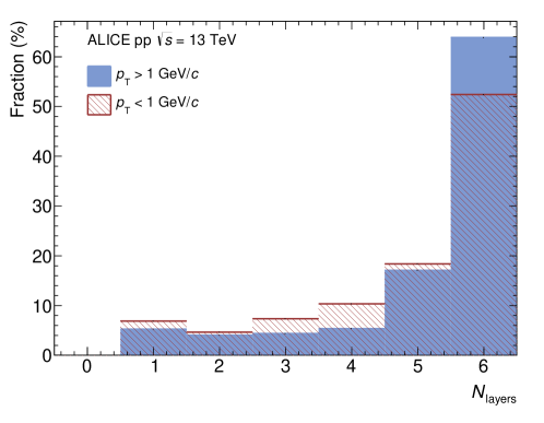
Figure 24: Fraction of tracks, originating from the primary vertex, consisting of a given number of layers in pp collisions at $\sqrt{s}=13~{}\mathrm{TeV}$.

A crucial figure of merit for the tracking is the fraction of global tracks matched to the TRD. This includes acceptance effects, between the TPC and the TRD as well as the TRD and the TOF detector. The momentum dependence is shown in Fig. 25 for tracks with at least 4 layers (about 75% of all tracks). For positively charged particles, the Lorentz drift of the electrons is opposite to the track inclination, which (together with the tail cancellation) results in a slightly higher efficiency.

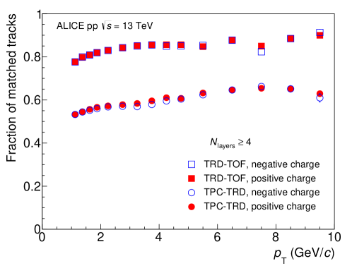
Figure 25: Fraction of tracks matched between the TPC and the TRD (TPC-TRD) and further the TOF detector (TRD-TOF) as a function of transverse momentum in pp collisions at $\sqrt{s}=13~{}\mathrm{TeV}$.

A systematic analysis of the position resolution in the bending plane ($r\varphi$) is presented in Fig. 26. The resolution ($\sigma_{\Delta y}$) is expressed as the width of a Gaussian fit to the difference between the position reconstructed via tracklets and different references ($\Delta y$). It is shown as a function of the inverse transverse momentum scaled with the particle charge ($q/p_{\mathrm{T}}$). First, the ideal position resolution is derived from Monte Carlo simulations by comparing the reconstructed tracklet position with the true particle position at the reference radial point (anode wire plane of the read-out chamber). This is shown as the red curve in Fig. 26, calculated in local chamber coordinates to decouple residual misalignment effects from the result. A parabolic best fit is performed for which the parameters show the best position resolution of close to $200\text{\,}\mathrm{\SIUnitSymbolMicro m}$ at $p_{\mathrm{T}}$ = 1.8 $\mathrm{GeV}\!/c$. The best performance is achieved for tracks where the inclination angle cancels the $E\times B$ effect. In the case of real data, the comparison can be performed only against a measured estimator, i.e. against the reconstructed global (ITS + TPC) track. The black curve shows the distribution for pp collisions at $\sqrt{s}=8~{}\mathrm{TeV}$. The combined position resolution of the TRD and global tracks is around $700\text{\,}\mathrm{\SIUnitSymbolMicro m}$ at very large transverse momentum. In order to bridge the two results, observables at the level of reconstruction and simulation are compared. The blue curve shows the position resolution of the global tracks as reconstructed against the true position from the Monte Carlo simulation. The green line represents the theoretical value for the combined resolution for TRD and global tracks, given by the quadratic sum of the dependencies described by the red and the blue distributions. These tracks from simulation yield a slightly worse resolution because the theoretical limit does not consider the pad tilting. It is worth noting that the simulated position resolution describes the measured dependency reasonably well. Effects of remaining miscalibration and misalignment of all central barrel detectors lead to a degradation of about $500\text{\,}\mathrm{\SIUnitSymbolMicro m}$ for the resolution in the TRD.

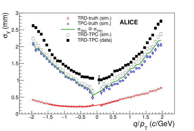
Figure 26: Dependence of the position resolution on charge over transverse momentum for simulated tracks in the TRD (red) and in the TPC (blue), reconstructed global tracks from simulation (gray) and from pp collisions at $\sqrt{s}=13~{}\mathrm{TeV}$ (black). The label TRD-TPC indicates global tracks reconstructed with the ITS and TPC that were extrapolated to the TRD. The green line represents the theoretical value for the combined resolution of TRD and global tracks. The red line shows a parabolic fit to the corresponding points.

The good position resolution capabilities demonstrated by the TRD detector can be used in the central barrel tracking of ALICE to improve the transverse momentum resolution of reconstructed particles. Figure 27 shows the $q/$$p_{\mathrm{T}}$ resolution of the combined ITS-TPC tracking with and without the TRD for various running scenarios. In all considered cases the TRD was also used as reference to obtain the correction maps for the distortions in the TPC. The inclusion of the TRD in tracking in addition improves the resolution by about 40% at high transverse momentum for pp collisions recorded at both low (12 kHz) and high interaction (230 kHz) rates. For example in the low interaction scenario of pp collisions, the achieved $p_{\mathrm{T}}$ resolution is 3% at 40 GeV. In addition the inclusion of the TRD in the track reconstruction improves the impact parameter resolution and the reconstruction of tracks that pass at the edges of the TPC sectors, i.e. increasing the acceptance of the experiment.

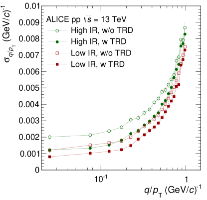
Figure 27: Improvement of the $q/$$p_{\mathrm{T}}$ resolution in data when TRD information is included as compared with the performance of tracking without TRD information for various running scenarios. The labels low and high IR indicate interaction rates of 12 and 230 kHz, respectively.

9 Alignment

The physical alignment of the detectors during installation (see Section 2.3) has a finite precision of the order of $1\text{\,}\mathrm{mm}$ for chambers within a supermodule and of $1\text{\,}\mathrm{cm}$ for supermodules in the spaceframe. The subsequent software alignment, i.e. accounting for the actual positions of supermodules and chambers in the reconstruction and simulation software, is the subject of this section. The alignment parameters (three shifts and three rotation parameters per alignable volume) are deduced from optical survey data and/or from reconstructed tracks. In the latter case, the obtained values have to be added to those already used during the reconstruction. The obtained alignment sets are stored in the OCDB and used in the subsequent reconstructions.

The different alignment steps are described in the following subsections. The alignment is checked and, if necessary, redone after shutdown periods and/or interventions that may affect the detector positions, e.g. installations of new supermodules.

9.1 Internal alignment of chambers with cosmic-ray tracks

The internal detector alignment, i.e. the relative alignment of the read-out chambers within one stack, is performed with cosmic-ray tracks recorded without magnetic field (Fig. 28, left).

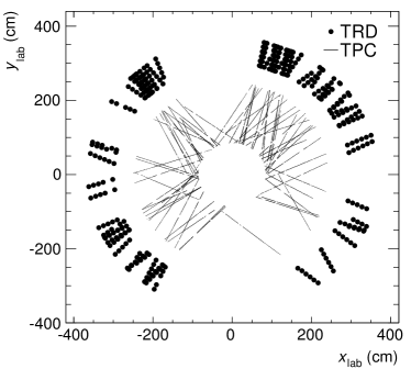
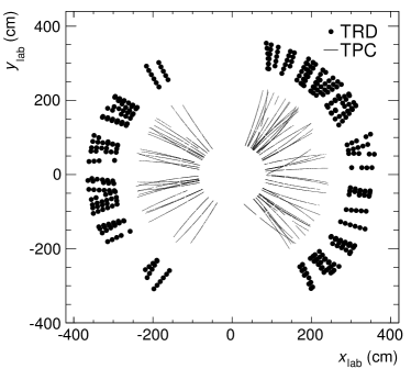
Figure 28: Left: Cosmic-ray tracks with at least 100 TPC clusters and 5 TRD layers, recorded without magnetic field, used for the relative $r\varphi$ alignment of the TRD chambers within stacks (internal alignment). Right: Charged-particle tracks with at least 100 TPC clusters and 4 TRD layers from pp collisions at $\sqrt{s}=8$ TeV, used for the alignment of the TRD with respect to the TPC (external alignment). Both figures show data from 2012 (setup with 13 supermodules).

The local $y$ coordinates (see Section 2) of the chambers of the intermediate layers L1–L4 (tracklet) are varied to minimise the $\chi^{2}$ of straight tracks calculated from the hits in layers L0 and L5. The coordinates of the first and last chamber, L0 and L5, are kept constant. Any misalignment of a stack, such as a tilt, possibly resulting from this constraint is removed later during the stack alignment. Chamber tilts are neglected. The typical spread (Gaussian $\sigma$) of the residual between tracklet and straight track is about $1\text{\,}\mathrm{mm}$ for a single chamber (see Table 5). The initial chamber misalignments of 0.6–$0.7\text{\,}\mathrm{mm}$ are reduced to 0.2–$0.3\text{\,}\mathrm{mm}$ (r.m.s.). The minimum required statistics is $O(10^{3})$ tracks per read-out chamber (i.e. per stack). For a few stacks, located around $\varphi=0$ and $\varphi$ = $180\text{\,}\mathrm{\SIUnitSymbolDegree}$, with low statistics of cosmic-ray tracks, charged tracks from pp collisions taken without magnetic field are used instead.

Alignment volumes	Input data set	Residual width ($\sigma$)
L0	cosmics	$2\text{\,}\mathrm{mm}$
L2	cosmics	$1\text{\,}\mathrm{mm}$
L5	cosmics	$2\text{\,}\mathrm{mm}$
L0	pp collisions	2–$3\text{\,}\mathrm{mm}$
L2	pp collisions	1–$2\text{\,}\mathrm{mm}$
L5	pp collisions	2–$3\text{\,}\mathrm{mm}$

Table 5: Typical width of the tracklet-to-track residuals in $y$ observed during the internal alignment procedure. The residuals are between a tracklet (measured by a single chamber) and track (defined by the remaining chambers of the stack). L0–L5 refer to the six TRD chambers within a stack. The L0 and L5 resolutions are given only for comparison purposes as the positions of these two chambers are fixed during the minimisation.

The internal $y$ alignment sets deduced from cosmic-ray tracks and from pp collisions agree within 0.18 mm (Gaussian $\sigma$). From this, the accuracy of the internal alignment is estimated to be about $\Delta y=0.18~{}{\rm mm}/\sqrt{2}=0.13~{}{\rm mm}$. Similar agreement exists between cosmic-ray runs taken in different periods.

9.2 Survey-based alignment of supermodules

The supermodules are subject to an optical survey after installation and, subsequently, after every hardware intervention that may affect the geometry of the detector. For this measurement, survey targets are inserted into precision holes existing at each end of every supermodule.

Because of poor accessibility of the muon-arm side, the supermodules are only surveyed on one side (A-side). Four of the six alignment parameters, $x$, $y$, $z$ shifts and the rotation around the $z$-axis, are then determined for each supermodule by fitting the survey results. The typical survey precision is $1\text{\,}\mathrm{mm}$. The survey-based alignment procedure reduces the supermodule misalignment from its initial value of 1–$2\text{\,}\mathrm{cm}$ to a few $\mathrm{mm}$.

9.3 External alignment with tracks from beam–beam collisions

The external alignment, i.e. the alignment of TRD volumes with respect to the TPC, is performed with charged-particle tracks recorded with magnetic field (Fig. 28, right). Only tracks with $p_{\mathrm{T}}>1.5~{}\mathrm{GeV}\!/c$ are used. First, all six alignment parameters of each TRD supermodule are varied to minimise the residuals. Subsequently, the alignment of each stack is refined by adjusting its $x$ and $y$ positions and its rotation around the $z$-axis. The tracklet-to-track residuals in $y$ before and after alignment are shown in Fig. 29 for two supermodules. As can be seen, the initial misalignment and the degree of improvement vary supermodule by supermodule. The typical width of the residuals (Gaussian $\sigma$) is about $2\text{\,}\mathrm{mm}$ (see Table 6). In the limit of low number of tracks per stack $N_{\rm track}$, the alignment precision is statistical: $\sigma/\sqrt{N_{\rm track}}$. With $N_{\rm track}=O(10^{3})$, systematic effects start to dominate.

Alignment volumes	Residual width ($\sigma$)
L0 chamber	$1\text{\,}\mathrm{mm}$
L5 chamber	$3\text{\,}\mathrm{mm}$
stack	$2\text{\,}\mathrm{mm}$
supermodule	$2\text{\,}\mathrm{mm}$

Table 6: Typical width of the tracklet-to-track residuals observed during the external alignment procedure with $p_{\mathrm{T}}>1.5$ $\mathrm{GeV}\!/c$ tracks from pp collisions. The residuals are between a TRD chamber, stack, or supermodule and the TPC track. L0 and L5 denote the first and the last (radially) TRD chambers within a stack.

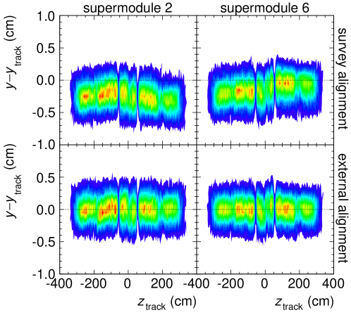
Figure 29: TRD tracklet to TPC track residuals in $y$ as a function of the $z$ coordinate of the TPC track ($z_{\rm track}$) for supermodules 2 (left) and 6 (right). The colour code is linear in the number of tracks. The upper and lower panels show the situation with the survey alignment and with in addition the external alignment, respectively. The data are from a 2012 run of pp collisions with B = $-$$0.5\text{\,}\mathrm{T}$. The alignment set used for the lower plots was deduced from the same run. The internal alignment is applied in all four cases.

Figure 29 shows the effect of an alignment procedure applied to the same data set from which it was deduced. However, one single alignment set is used for runs of a complete year. This raises the question of the universality and temporal stability of the alignment, which can be addressed by comparing alignment sets deduced from various portions of data. Separate analyses of positive and negative tracks yield two alignment sets that agree within $1\text{\,}\mathrm{mm}$ (r.m.s. of the $y$ shifts). A larger difference ($2\text{\,}\mathrm{mm}$) is seen between the two magnetic field polarities. Such differences can result from mechanical displacements and/or from the fact that the TPC calibration is performed separately for the two polarities. The presence of a step in the middle of the central TRD stack, at $z=0$, in Fig. 29 indicates the latter. Several iterations of the TRD to TPC alignment and the TPC calibration with respect to the TRD are needed to achieve the best possible precision. In order to address the entanglement of the alignment and calibration of the central barrel detectors, an alternative approach was developed during LS 1. It is based on a combined alignment and calibration fit performed using the Millepede algorithm [99]. The new method allows for a simultaneous alignment and calibration of the ITS, TRD, and TOF, followed by the calibration of the TPC. The procedure is being used successfully in Run 2.

10 Calibration

The ALICE calibration scheme is explained in [2]. Here the calibration procedures for the TRD are described. The four basic calibration parameters for the TRD – time offset, drift velocity, gain, and noise – are illustrated in Fig. 30. The position of the anode wires and the entrance window are visible in the measured drift time spectrum as a peak (around $0.5\text{\,}\mathrm{\SIUnitSymbolMicro s}$, caused by charges coming from both sides of the anode wires) and an edge (around $2.8\text{\,}\mathrm{\SIUnitSymbolMicro s}$), respectively. Since the calibrated time represents the distance from the anode wires, the position of the anode peak provides the time offset. The time span between the anode peak and the entrance-window edge is inversely proportional to the drift velocity. The mean pulse height is proportional to the gain and the width of the pedestal is proportional to the pad noise.

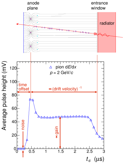
Figure 30: Average pulse height vs. drift time plot (derived from Fig. 5) illustrating the main calibration parameters. For better understanding, a sketch of the chamber cross-section with field lines from Fig. 2 is shown at the top. The peak at the left and the edge on the right of the drift time spectrum correspond to the anode wires and the chamber entrance window. The temporal difference between them depends on the drift velocity. The anode-peak position defines the time offset. The mean pulse height and the pedestal width are related to the gain and the pad noise, respectively.

While ionisation electrons are attracted to the anode wires by an electric field $E$, the presence of a magnetic field perpendicular to it, $|E\times B|>0$, leads to a Lorentz angle of about 9^∘ between the electron drift direction and the direction of the electric field. Knowledge of the Lorentz angle is necessary for the reconstruction of the tracklets, described in Section 8.2 (see Fig. 22 and Fig. 46).

The complete list of the calibration parameters, organised according to the source from which they are determined, is given in Table 7.

Input data	Parameters
pedestal runs	pad noise, pad status
runs with ${}^{83{\rm m}}{\rm Kr}$ in the gas	relative pad gain
physics runs (cpass0/1)	chamber status, time offset, drift velocity, Lorentz angle, gain

Table 7: Sources of input data and the derived calibration parameters.

Once determined for a given run, the calibration parameters are stored in the OCDB and used in the subsequent reconstructions. In the following, the methods used to determine the values of the calibration parameters are discussed.

10.1 Pad noise and pad status calibration using pedestal runs

Short pedestal runs are taken roughly once per month during data taking. In these runs, events are triggered at random instants and the data are recorded without zero suppression. At the end of the run, an automatic analysis of the pedestal data is performed on the computers of the DAQ system [100]. Hundred events are sufficient to calculate the position of the baseline of the analogue pre-amplifier and shaper output (pedestal) and its fluctuation (noise) for all electronics channels. The results are subsequently collected by the Shuttle system [87] and transported to the OCDB. The mean noise is 1.2 ADC counts, corresponding to an equivalent of 1200 electrons. The pad-by-pad r.m.s. value is 0.17 counts. The precision of the measurement is 0.015 counts (r.m.s.). Pads that have a faulty connection to the FEE, are connected to a non working FEE channel, have excessive noise, or are bridged with a neighbour are marked in the OCDB and treated correspondingly during the data taking and reconstruction chain (pad status).

10.2 Pad gain calibration using ${}^{83{\rm m}}{\rm Kr}$ decays

Pad-by-pad gain calibration of the TRD chambers is performed after every installation of new supermodules. It is done by injecting radioactive gas into the chambers and measuring the signals of the decay electrons. The method, developed by ALEPH [101, 102] and DELPHI [103], is also used to calibrate the ALICE TPC [31].

Solid ⁸³Rb decays by electron capture into gaseous Kr and populates, among others, the isomeric state ${}^{83{\rm m}}{\rm Kr}$ with an excitation energy of $41.6\text{\,}\mathrm{keV}$ and a half-life of 1.8 hours. The radioactive krypton is injected into the gas circulation system and is distributed over the sensitive volumes of all installed chambers. The krypton nuclei decay to their ground state by electron emission. The decay energy, comparable to the energy lost by a minimum-ionising particle traversing the sensitive volume of a read-out chamber (20–$30\text{\,}\mathrm{keV}$), gets deposited within $1\text{\,}\mathrm{cm}$ from the decay point. For each decay, the total signal is calculated by integrating over $y$ (pad column), $z$ (pad row) and $x$ (drift time), and filled into the histogram associated with the pad of maximum signal.

With three gas inlets to each supermodule (see Section 3), groups of 10 chambers are connected in series. The difference between the decay rates seen in the first and last chamber of the chain was reduced to a factor of ${\sim}$3 by increasing the gas flow during the krypton calibration run. With an ⁸³Rb source intensity of $5\text{\,}\mathrm{MBq}$ and a measurement time of one week, the collected statistics is of the order of thousand counts per pad. This is sufficient to identify the expected decay lines in the distribution. An example is shown in Fig. 31. The histogram of each pad is fitted by stretching horizontally the reference distribution. The stretching factor is the measure of the pad gain. The energy resolution at $41.6\text{\,}\mathrm{keV}$ is 10%.

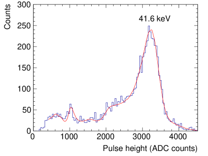
Figure 31: Pulse height spectrum accumulated for one pad during the Kr-calibration run [104, 105]. The smooth solid line represents the fit from which the gain is extracted.

The resulting pad gain factors for one particular chamber are shown in Fig. 32.

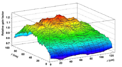
Figure 32: Relative pad gains for one chamber calibrated with electrons from ${}^{83{\rm m}}{\rm Kr}$ decays.

The short-range variations of up to 10% reflect the differences between electronics channels. The long-range inhomogeneities originate from chamber geometry and are typically within $\pm$15% (peak to peak). A detailed description of the krypton calibration can be found in [104] and [105].

The improvement of the chamber resolution achieved by the krypton-based pad-by-pad calibration is presented in Fig. 33. The histograms show the pulse height spectrum before calibration, after one and after two iterations (calibrations performed in consecutive years), respectively.

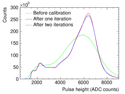
Figure 33: Pulse height spectrum before the krypton-based calibration, after one and after two iterations (calibrations performed in consecutive years) for one read-out chamber.

10.3 Chamber calibration using physics data

The anode and drift voltages of the individual chambers are adjusted periodically (once a year) to equalise the chamber gains and drift velocities. Moreover, an automatic procedure is in place that continuously adjusts the voltages depending on the atmospheric pressure, compensating the impact of the environment on the gas properties (see Section 7.2). This is important because the pulse height and the tracklet angle are used for triggering (see Section 12).

In order to achieve the ultimate resolution for physics data analysis, the chamber status, time offset, drift velocity, Lorentz angle, and gain are calibrated run-by-run offline, using global tracks from physics runs. A sample of events of each run is reconstructed for this purpose. The required statistics is equivalent to $10^{5}$ pp interaction events. The first reconstruction pass (cpass0) provides input for the calibration. The second pass (cpass1) applies the calibration and the reconstructed events are used as input for the data quality assurance analysis, and for the second iteration of the calibration. The read-out chamber status and the chamber-wide time offset, drift velocity, Lorentz angle, and gain values are extracted from cpass0 and updated after cpass1. The time offset is obtained as indicated in Fig. 30. The drift velocity and the Lorentz angle are derived from the correlation between the derivative of the local tracking $y$ coordinate with respect to the drift time, and the azimuthal inclination angle of the global track (see Fig. 34). The former represents the uncalibrated estimate of the tracklet angle. The latter is obtained from the extrapolation of the global track to the TRD. The correlation is fitted by a straight line. The effect of the pad tilt ($\mathrm{d}y/\mathrm{d}z=\tan(\alpha)$, $\alpha=\pm$ $2\text{\,}\mathrm{\SIUnitSymbolDegree}$, see Section 2) is taken into account by adding the respective term to the global track inclination. The slope and the offset parameters give the drift velocity and the Lorentz angle, respectively.

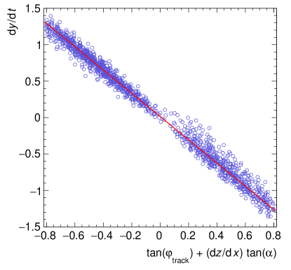
Figure 34: The derivative of the local tracking $y$ coordinate with respect to the drift time $t$ vs. the tangent of the azimuthal track inclination angle from global tracking. The slope and the offset of the fit (red line) give the drift velocity and the Lorentz angle, respectively.

The gain calibration factor is determined by histogramming, for each chamber, the deposited charge divided by the path length and taking the mean of this distribution. The last stage of the chamber calibration is to identify chambers for which a satisfactory calibration cannot be obtained or whose parameter values are very different from the mean. These chambers are masked in the data analysis and in the respective simulation.

The typical mean values, chamber-by-chamber variations, stability, and precision of the calibration parameters are shown in Table 8.

Parameter	Mean	Variations	Stability	Precision
$t_{\mathrm{0}}$	$145.2\text{\,}\mathrm{ns}$	$2.7\text{\,}\mathrm{ns}$	$\pm$$3.4\text{\,}\mathrm{ns}$	$1\text{\,}\mathrm{ns}$
$v_{\mathrm{d}}$	$1.56\text{\,}\mathrm{c}\mathrm{m}\mathrm{/}\mathrm{\SIUnitSymbolMicro}\mathrm{s}$	1–14%	$\pm$3%	0.4%
$\Psi_{\rm L}$	$8.8\text{\,}\mathrm{\SIUnitSymbolDegree}$	$0.3\text{\,}\mathrm{\SIUnitSymbolDegree}$–$0.5\text{\,}\mathrm{\SIUnitSymbolDegree}$	$\pm$$0.4\text{\,}\mathrm{\SIUnitSymbolDegree}$	$0.05\text{\,}\mathrm{\SIUnitSymbolDegree}$
gain	1.0 (a.u.)	3–16%	$\pm$7%	1.4%

Table 8: The typical mean values, chamber-by-chamber variations, stability (in the second half of 2012), and precision of the chamber calibration parameters $t_{\mathrm{0}}$ (drift time offset), $v_{\mathrm{d}}$ (drift velocity), $\Psi_{\rm L}$ (Lorentz angle for $B$ = $0.5\text{\,}\mathrm{T}$), and gain. For the chamber-by-chamber variations, which are subject to equalisation by adjusting the voltages, ranges are indicated.

The chamber-by-chamber variation is quantified by the r.m.s. of the chamber distribution within one run. The stability is described via the maximum variations observed in one read-out chamber during half a year of running. The precision is defined as 1/$\sqrt{2}$ of the r.m.s. difference between the calibration parameters deduced from two high-statistics data sets taken under identical conditions.

10.4 Quality assurance

As described before, during cpass1 reconstructed events are subject to a quality assurance (QA) analysis in which control histograms monitoring the quality of the calibrated data are filled. The analogous monitoring of raw data, performed online, is described in Section 7.3. As an example, two such QA histograms, representing the efficiency and the mean number of layers in each stack (equivalent to the number of active layers) in one particular run of the pp data taking in 2015, are shown in Fig. 35. The efficiency drops at stack boundaries and the window in correspondence of the detector coverage of the PHOS detector are visible.

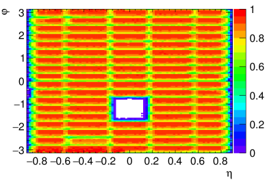
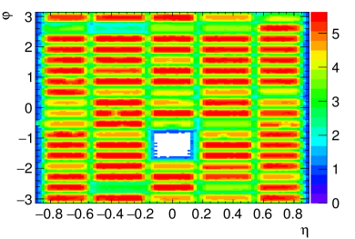
Figure 35: Two quality-assurance plots (data from pp collisions recorded in 2015 with all supermodules installed, tracks with at least 70 TPC clusters and $p_{\mathrm{T}}>0.5$ $\mathrm{GeV}\!/c$). Left: Efficiency of matching tracklets to TPC tracks. Right: Mean number of layers per track in each stack (cf. the discussion of inactive chambers in Section 7.2).

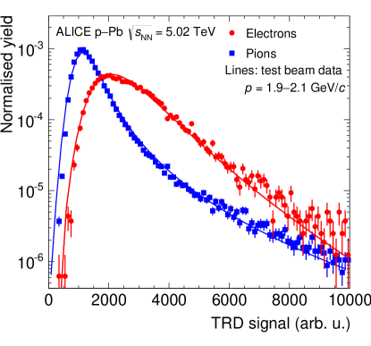
Figure 36: Total integrated charge, normalised to the tracklet length, measured in a single read-out chamber for electrons and pions in p–Pb collisions at $\sqrt{s_{\mathrm{NN}}}$ = 5.02 TeV, in comparison with results from test beam measurements (solid lines) [47, 106]. The electrons and pions from test beam measurements were scaled by one common factor to compensate the difference in gain of the two data sets.

11 Particle identification

The TRD provides electron and charged hadron identification based on the measurement of the specific energy loss and transition radiation. The total integrated charge measured in a tracklet [107], normalised to the tracklet length, is shown in Fig. 36 for electrons and pions in p–Pb collisions at $\sqrt{s_{\mathrm{NN}}}$ = 5.02 TeV. The electron and pion samples were obtained by selecting tracks originating from $\gamma\rightarrow e^{+}e^{-}$ conversions in material and from the decay K${}^{0}_{\rm s}\rightarrow\pi^{+}\pi^{-}$ via topological cuts and particle identification (PID) with the TPC and the TOF. The obtained electron sample has an impurity of less than 1%. Due to the larger specific energy loss and transition radiation, the average charge deposit of electrons is higher than that of pions. Charge deposit distributions recorded in test beam measurements at CERN PS in 2004 for electrons and pions in the momentum range 1 to 10  $\mathrm{GeV}\!/c$ [47, 106] describe the results from collision data well (see Fig. 36), and can thus also be used as references for particle identification.

The measured charge deposit distributions can be fitted by a modified Landau-Gaussian convolution: (Exponential $\times$ Landau) $\ast$ Gaussian [108, 109], where the Landau distribution is weighted by an exponential dampening (Landau$(x)~{}\rightarrow~{}e^{kx}$ Landau$(x)$). This function describes the specific charge deposit distributions for pions ($\mathrm{d}E/\mathrm{d}x$) and electrons ($\mathrm{d}E/\mathrm{d}x$ + TR) well and can thus be used to extract the most probable energy loss. The dependence of the most probable signal versus $\beta\gamma$ is shown in Fig. 37.

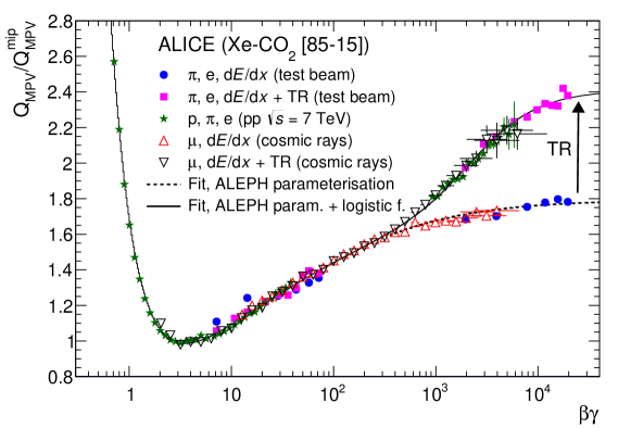
Figure 37: Most probable charge deposit signal normalised to that of minimum ionising particles as a function of $\beta\gamma$. The data are from measurements performed in test beam runs, pp collisions at $\sqrt{s}$ = 7 TeV, and cosmic-ray runs. Uncertainties in momentum and thus $\beta\gamma$ determination are drawn as horizontal and statistical uncertainties as vertical error bars. The shown fits correspond to the Equations 1 and 2 described in the text.

The data have been extracted from measurements (i) in a beam test at CERN PS in 2004 (pions and electrons) [106], (ii) with pp collisions at $\sqrt{s}=7$ TeV (protons, pions and electrons) [107] and (iii) with a cosmic-ray trigger in the ALICE setup (muons) [108]. The selection of the flight direction of the cosmic-ray muons allows only the specific energy loss ($\mathrm{d}E/\mathrm{d}x$) or the summed signal ($\mathrm{d}E/\mathrm{d}x$ + TR) to be measured by selecting muons that first traverse the drift region and then the radiator, and vice versa [108, 109]. To improve the momentum reconstruction of very high $p_{\mathrm{T}}$ cosmic-ray muons, a dedicated track fitting algorithm [108, 109] was developed, combining the clusters of the two individual tracks in the two hemispheres of the TPC. This yields a better momentum resolution by about a factor of 10, e.g. at 1 TeV$/c$ the 1/$p_{\mathrm{T}}$ resolution is 8.1$\cdot 10^{-4}$ (GeV/$c$)^-1 [108, 109].

The onset of the TR production is visible for $\beta\gamma\gtrsim 800$, both for electrons and high-energy (TeV scale) cosmic-ray muons. The signals for muons are consistent with those from electrons at the same $\beta\gamma$. The most probable signal (MPV) of the energy loss due to ionisation only, normalised to that of minimum ionising particles (mip), is well described by the parameterisation proposed by the ALEPH Collaboration [101, 110] (shown in Fig. 37):

$$\left(\frac{Q_{\rm MPV}}{Q_{\rm MPV}^{\rm mip}}\right)=0.2\cdot\frac{4.4-\beta^{2.26}-\ln\left[0.004-\frac{1}{\left(\beta\gamma\right)^{0.95}}\right]}{\beta^{2.26}}.~{}~{}$$ (1)

Minimum ionising particles are at a $\beta\gamma$ value of 3.5 and the $\mathrm{d}E/\mathrm{d}x$ in the relativistic limit is 1.8 times the minimum ionisation value. To describe the $\mathrm{d}E/\mathrm{d}x$ + TR signal, a parameterised logistic function is needed in addition. The formula, normalised to the signal for minimum ionising particles, is as follows:

$$\frac{\rm TR}{\rm TR^{\rm mip}}=\frac{0.706}{1+\exp(-1.85\cdot(\ln\gamma-7.80))}.$$ (2)

The saturated TR yield in the relativistic limit is 0.7 times the minimum ionisation value. At $\beta\gamma$ = $2.4\cdot 10^{3}$ the logistic function reaches half its maximum value.

11.1 Truncated mean method

The TRD can provide electron (described in the next section) and hadron identification. For the hadron identification, the truncated mean is calculated from the energy loss (+TR) signal stored in the clusters (see Section 8) [108]. For the particle identification, the deviation from the expected most probable signal for a given species is then used after normalisation to the expected resolution of the truncated mean signal for the track under study.

In order to obtain an approximately Gaussian shape, the long tail of the Landau distribution needs to be eliminated or at least strongly suppressed, which can be realised through a truncated-mean procedure. The PID signal of a charged hadron passing through the detector is calculated using all $M$ clusters along the up to six layers (see Section 8). The truncated mean is then calculated as the average over the $N$ lowest values: $N=f\cdot M$. The truncation fraction $f$ = 0.55 was chosen in order to maximise the separation power between minimum ionising pions with $p$ = 0.5 $\mathrm{GeV}\!/c$ and electrons with $p$ = 0.7 $\mathrm{GeV}\!/c$. The different momenta were chosen to maximise the statistics of the electron sample [108]. However, the cluster signal strength depends on the radial position of the cluster within the read-out chamber (see Fig. 5). Therefore, the cluster amplitudes are first weighted with time-bin dependent calibration factors, found and applied during the cpass0/cpass1 calibration steps (see Section 10). For example, for the cosmic-ray data sample, the weights are determined for tracks within the interval $1.65\leq{\rm log}_{10}(\beta\gamma)\leq 2.5$ to eliminate kinematic dependences. These $\beta\gamma$ are far below the onset of TR. After applying this procedure, some non-uniformity over time bins remains ($\pm$15%), which is due to the TR component [108].

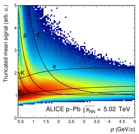
Figure 38: Truncated mean signal as a function of momentum for p–Pb collisions at $\sqrt{s_{\mathrm{NN}}}$ = 5.02 TeV. The solid lines represent the expected signals for various particle species.

Figure 38 shows the truncated mean signal as a function of momentum for p–Pb collisions at $\sqrt{s_{\mathrm{NN}}}$ = 5.02 TeV. The curves represent the expected signals for various particle species. These parameterisations were obtained by fitting the truncated mean signal ($\mathrm{d}E/\mathrm{d}x$ + TR) of electrons from conversion processes, pions from K${}^{0}_{\rm s}$ and protons from $\Lambda$ decays as a function of $\beta\gamma=\frac{p}{m}$ with a sum of the ALEPH parameterisation (Eq. 1) and logistic function (Eq. 2), see above.

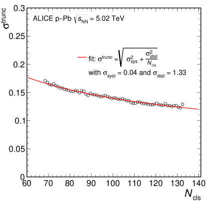
Figure 39: Resolution of the truncated mean signal as a function of the number of clusters in p–Pb collisions at $\sqrt{s_{\mathrm{NN}}}$ = 5.02 TeV.

The resolution of the truncated mean signal is shown in Fig. 39 as a function of the number of clusters ($N_{\rm cls}$), which is described by the function

$$\sigma^{\rm trunc}=\sqrt{\sigma_{\rm sys}^{2}+\frac{\sigma_{\rm stat}^{2}}{N_{\rm cls}}},$$ (3)

where $\sigma_{\rm sys}$ describes systematic uncertainties due to, e.g. residual calibration effects. The fit shows that the resolution is, as expected, mainly driven by a statistical scaling according to the law $\sigma^{\rm trunc}\propto 1/\sqrt{N_{\rm cls}}$. The results demonstrate a resolution of the truncated mean signal of 12% for tracks with signals in all six layers. It should be noted that the resolution is, in parts, limited by the ion tails in the late time bins leading to a correlation between individual time bins (see Section 8).

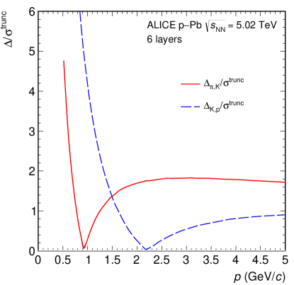
Figure 40: Measured separation power ($\frac{\Delta}{\sigma^{\rm trunc}}=\frac{S^{\rm trunc}_{\pi\rm,K}-S^{\rm trunc}_{\rm K,p}}{\sigma^{\rm trunc}}$) for $\pi$/K and K/p separation as a function of momentum.

Figure 40 shows the pion-kaon and kaon-proton separation power as a function of momentum. The separation power is calculated as the distance between the expected truncated mean signal $S^{\rm trunc}$ of pions (kaons) and kaons (protons) divided by the resolution of the response: $\frac{\Delta}{\sigma^{\rm trunc}}=\frac{S^{\rm trunc}_{\pi\rm,K}-S^{\rm trunc}_{\rm K,p}}{\sigma^{\rm trunc}}$. At low momenta an excellent separation power is achieved, at high momentum the separation power is about 2 for $\pi$/K and 1 for K/p.

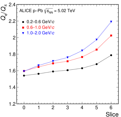
Figure 41: Ratio of the average signal of electrons to that of pions as a function of the depth in the detector (slice number; the lowest (highest) slice number is farthest away from (closest to) the radiator).

11.2 Electron identification

For the electron identification (eID), also the temporal evolution of the signal is used. For each TRD chamber the signal amplitudes of the clusters along a tracklet are redistributed into seven slices during the track reconstruction (see Section 8). Each slice corresponds to about 5 mm of detector thickness for a track with normal incidence. The ratio of the average signal for electrons and pions as a function of the slice number is shown in Fig. 41 for p–Pb collisions at $\sqrt{s_{\mathrm{NN}}}$ = 5.02 TeV. At large slice numbers, i.e. long drift times, the TR contribution is visible because the TR photon is predominantly absorbed at the entrance of the drift region.

The eID performance is expressed in terms of the electron efficiency (the probability to correctly identify an electron) and the corresponding pion efficiency (the fraction of pions that are incorrectly identified as electrons). The inverse of the pion efficiency is the pion rejection factor. The following methods are in use: i) truncated mean (see previous section), ii) a likelihood method with ‘dimensionality’ (one-dimensional, LQ1D, corresponds to the total integrated charge [107], two-dimensional, LQ2D, for two charge bins [111], etc.), iii) neural networks (NN) [112, 113, 114].

For the LQ2D method the signal is evaluated in two charge bins, i.e. the integrated signals of the first four slices and the last three slices are averaged. The latter sum contains most of the TR contribution. For the LQ3D method, the signals of the slices are combined as sums of the first three, the next two and the final two. Both the LQ7D and NN methods utilise 7 charge bins and thus benefit from the complete information contained in all 7 slices. While individual slices may be empty, the charge bins must contain a charge deposition. In physics analyses, this selection criterion does not introduce a loss of electrons when applying the LQ1D or the LQ2D methods, but causes a reduction in the number of electrons by about 40% when the LQ7D method is used. The clean samples of electrons and pions described above are used to obtain references in momentum bins for particle identification. For each particle traversing the TRD, the likelihood values for electrons and pions, muons, kaons and protons are then calculated for each chamber via interpolation between adjacent momentum references. The global track particle identification is finally determined as the product of the single layer likelihood values. In physics analyses, hadrons (e.g. pions) can be rejected with the TRD by applying either a cut on the likelihood or a pre-calculated momentum-dependent cut on the likelihood value for electrons. The latter provides a specified electron efficiency constant versus momentum. To cross-check the references and determine systematic uncertainties, electrons from photon conversions can be studied. In Pb–Pb collisions the mean of the charge deposit distributions shows a centrality (event multiplicity) dependence, of about 15% comparing central and peripheral collisions [111], and therefore centrality-dependent references were introduced.

The references can only be created after the relative gain calibration of the individual pads and the time-dependent gain calibration of the chambers as described in Section 10. After this, the detector response is uniform across the acceptance and in time, and thus it can be studied in detail by combining all chambers and the full statistics of 1–2 months of data taking. Since the reference creation requires a large data sample, the reference distributions are only produced after the full physics reconstruction pass. This means that the reference creation can only be done later, during data analysis rather than already during reconstruction. The references for the truncated mean and the likelihood methods are stored for this purpose in the Offline Analysis Database (OADB) and read from there in the initialisation phase of the analysis tasks [115].

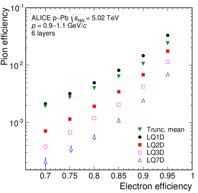
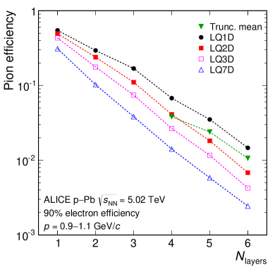
Figure 42: Pion efficiency as a function of electron efficiency (left, for 6 detector layers) and as a function of the number of detector layers (right, for 90% electron efficiency) for the various eID methods. The results are compared for the momentum interval 0.9–1.1 $\mathrm{GeV}\!/c$ in p–Pb collisions at $\sqrt{s_{\mathrm{NN}}}$ = 5.02 TeV. The results of the truncated mean method are only shown for a minimum of 4 tracklets, where the resolution is better than 18% (see Fig. 39).

The pion efficiency for 1 $\mathrm{GeV}\!/c$ tracks is shown as a function of the electron efficiency and as a function of the number of detector layers providing signals for the various methods in Fig. 42. For all methods the pion rejection factor decreases as expected with decreasing number of contributing layers and a lower electron selection efficiency corresponds to a better pion rejection factor for all methods.

A pion rejection factor of about 70 is obtained at a momentum of 1 $\mathrm{GeV}\!/c$ in p–Pb collisions with the LQ1D method, the most simple identification algorithm. The LQ2D method yields a pion rejection factor far better than the design goal of 100 at 90% electron efficiency found in test beams with prototypes [106]. When using the temporal evolution of the signal even better performance is achieved, reaching a rejection of up to 410.

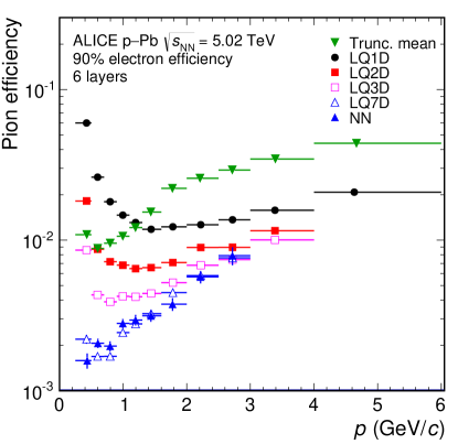
Figure 43: Pion efficiency (for 90% electron efficiency) as a function of momentum for the truncated mean, LQ1D, LQ2D, LQ3D, LQ7D and NN methods. The results are from p–Pb collisions at $\sqrt{s_{\mathrm{NN}}}$ = 5.02 TeV and for tracks with signals in six layers.

Figure 43 shows the momentum dependence of the pion efficiency for the different methods. At low momenta, the pion rejection with the LQ1D method improves with increasing momentum because of the onset of the transition radiation. From 1–2 $\mathrm{GeV}\!/c$ upwards, the electron–pion separation power gradually decreases due to the saturation of the TR production and the relativistic rise of the specific energy loss of pions. The other methods that make use of the temporal evolution of the signal provide substantial improvements, in particular for low and intermediate momenta. At high momenta (beyond 2 $\mathrm{GeV}\!/c$), the limitation in statistics for the reference distributions is reflected in the rather modest improvements in the pion rejection in the muti-dimensional methods. The similar momentum-dependent shape of the likelihood methods is in parts due to the usage of the same data sample for reference creation. The best performance is achieved for the LQ7D and NN methods. However these methods are sensitive to a residual miscalibration of the drift velocity, while the truncated mean and LQ1D method are more robust against small miscalibration effects. At low momentum, where the energy loss dominates the signal, the truncated-mean method provides very good pion rejection. The rejection power of the method decreases at higher momenta, because the TR contribution, yielding higher charge deposits, is likely to be removed in the truncation [108].

To visualise the strength of the TRD LQ2D electron identification method, the difference in units of standard deviations between the measured TPC energy loss of a given track and the expected energy loss of an electron for tracks with TOF and TOF+TRD particle identification is shown in Fig. 44. The results are compared for tracks with a momentum of 1.9–2.1 $\mathrm{GeV}\!/c$ within the TRD acceptance. In this momentum interval electrons cannot be discriminated from pions using TOF-only electron identification. After applying the TRD electron identification with 90% electron efficiency with the LQ2D method, hadrons are suppressed by about a factor of 130. The electron identification capabilities of the TRD thus allow selecting a very pure electron sample. This is important, e.g. for the measurement of electrons from heavy-flavour hadron decays. Details on the usage of the electron identification for the latter measurement in pp collisions at $\sqrt{s}$ = 7 TeV can be found in [116].

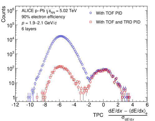
Figure 44: Difference in units of standard deviations between the measured TPC energy loss of a given track and the expected energy loss of an electron with TOF ($\pm 3\sigma^{\mathrm{TOF}}_{\mathrm{e}}$) and TRD (90% electron efficiency) electron identification. The distributions are shown for tracks with a momentum of 1.9–2.1 $\mathrm{GeV}\!/c$ within the TRD acceptance (6 layers in the TRD) in p–Pb collisions at $\sqrt{s_{\mathrm{NN}}}$ = 5.02 TeV.

In the Bayesian approach within ALICE [117], where the identification capabilities of several detectors are combined, the TRD particle identification contributes with its estimate of the probability for a given particle to belong to a given species. For this purpose, transverse momentum dependent ‘propagation factors’ for the priors, which represent the expected abundance of each particle species within the ITS and TPC acceptance, are calculated and stored in the analysis framework.

12 Trigger

ALICE features a trigger system with three hardware levels and a HLT farm [2]. Apart from the contributions from the pretrigger system (see Section 5.1), the TRD contributes to physics triggers at level-1. These are based on tracks reconstructed online in the GTU (see Section 5.3). The reconstruction is based on online tracklets (track segments corresponding to one read-out chamber) that are calculated locally in the FEE of each chamber. The local tracking in the FEE and the global online tracking in the GTU are discussed in the following.

As the trigger decision is based on individual tracks, a variety of signatures can be implemented, only limited by the complexity of the required calculations and the available time. In the following, the triggers on cosmic-ray muons, electrons, light nuclei, and jets are discussed.

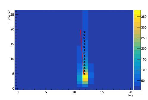
Figure 45: Example tracklet in one MCM. The ADC data for 26 time bins (100 ns each) from 21 channels are shown. The found clusters are marked as asterisks and the final tracklet, calculated as a straight line fit through the clusters, with Lorentz correction as a red line.

12.1 Local online tracking

The local online tracking is carried out in parallel in the FEE (see Section 5.2). Each of the $65\,000$ MCMs processes data from 21 pads, 3 of which are cross-fed from the neighbouring chips to avoid inefficiencies at the borders of the chip (see Fig. 15). For accurate online tracking, all relevant corrections and calibration steps must be applied online. After appending two digits to avoid rounding imprecisions, the digitised data are propagated through a chain of filters. First, a pedestal filter is used to compensate for variations in the baseline. A gain filter makes it possible to correct for local gain variations, either caused by the chamber or by the electronics. This equilibration is important for the evaluation of the specific energy loss, which is used for online particle identification. It uses correction factors derived from the krypton calibration (see Section 10.2). A tail cancellation filter can be used to reduce the bias from ion tails of signals in preceding time bins. This improves the reconstruction of the radial cluster positions and of the deflection in the transverse plane. The offline reconstruction takes the already applied online corrections into account. For that purpose, all configuration settings are stored in the OCDB and are, therefore, known during the offline processing.

After the filtering, the data for one event are searched time bin-wise for clusters by a hardware pre-processor. A cluster is found if the charge on three adjacent pads exceeds a configurable threshold and the center channel has the largest charge (see Fig. 45). For each MCM and time bin, transverse positions are calculated for up to six clusters. They are used to calculate and store the (channel-wise) sums required for a linear regression.

After the processing of all time bins, up to four channels with a minimum number of found clusters are further processed (if more than four channels exceed the threshold, the four of them with the largest number of clusters are used). For the selected channels, a straight line fit is computed from the pre-calculated sums. The fit results in information on the local transverse position $y$, the deflection in the bending plane $d_{y}$, the longitudinal position $z$, and a PID value. The transverse position and deflection are calculated from the fit, the longitudinal position is derived from the MCM position, and the PID from a look-up table using the accumulated charge as input.

The reconstructed values for $y$ and $d_{y}$ are corrected for systematic shifts caused by the Lorentz drift and the pad tilt. An example of a reconstructed tracklet is shown in Fig. 46. Eventually, the values (in fixed-point representation) are packed into one 32-bit word per tracklet for read-out.

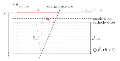
Figure 46: Sketch of the tracklet reconstruction. The tracklet reconstruction in the MCMs is performed in a local coordinate system. The tracklet comprises the information on $y$, $d_{y}$, $z$ and PID. The magnetic and electric field and the effect of the Lorentz angle ($\Psi_{\rm L}$) are indicated as well.

A realistic simulation of the local tracking was implemented in the ALICE software framework and is used in Monte Carlo productions based on event generators but can also be run on data recorded with the actual detector. This allows cross-validating hardware and simulation, and to study the effect of parameter changes on the tracklet finding. Therefore, Monte Carlo simulations are well-suited to study the performance of the online tracking algorithm with a given set of configuration options since tracklets can be compared to track references (track positions from Monte Carlo truth information). This allows tracklet efficiencies to be determined. An example is displayed in Fig. 47, which shows the efficiency of the tracklet finding process for a typical set of parameters as a function of $y$ and $q/p_{\mathrm{T}}$. The efficiency drops for large $y$ and negative $q/p_{\mathrm{T}}$, where the asymmetry in $y$ is caused by a combination of the Lorentz correction and the numerical range available for the deflection. The efficiency is close to 100% in the regime relevant for triggering. Furthermore, shifts in $y$ and $d_{y}$ are calculated with respect to the expectation from the Monte Carlo information. Besides a small systematic shift because of the uncorrected misalignment, the distributions show widths of about $300\text{\,}\mathrm{\SIUnitSymbolMicro m}$ and $1700\text{\,}\mathrm{\SIUnitSymbolMicro m}$ in $y$ and $d_{y}$ [71], respectively.

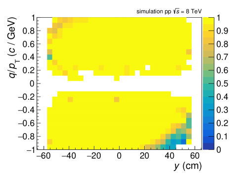
Figure 47: Reconstruction efficiencies for tracklets as a function of $y$ and $q/p_{\mathrm{T}}$ for Monte Carlo simulations. The $z$-axis entries are zero-suppressed.

12.2 Global online tracking

The global online tracking in the GTU operates stack-wise on the tracklets reconstructed and transmitted by the FEE. It is divided into a track matching and a reconstruction stage. The algorithm used for the matching of the tracklets is optimised for the high multiplicity environment of Pb–Pb collisions [118]. It is implemented in the FPGAs of the GTU (see Section 5.3) and operates in parallel on subsets of tracklets that are compatible with a track in the $x$-$z$ plane. Groups of tracklets which fall into ‘roads’ pointing to the nominal primary vertex are pre-selected. The tracklets are propagated to a virtual plane in the middle of the stack. Those which are close enough on this plane are considered to belong to the same track. The algorithm exploits a fixed read-out order of the tracklets to limit the number of comparisons for the matching, meaning that a linear scaling of the tracking time with the number of tracklets can be achieved.

Global online tracks consist of at least four matching tracklets. The reconstruction stage uses the positions of the contributing tracklets to calculate a straight line fit (see Fig. 48). The computation is simplified by the use of pre-calculated and tabulated coefficients, which depend on the layer mask. The approximation of a straight line is adequate for the trigger-relevant tracks above 2 $\mathrm{GeV}\!/c$. The transverse offset $a$ from the nominal vertex position is then used to estimate the transverse momentum [118]. The PID value for the track is calculated as the average over the contributing tracklets. A precise simulation of all the tracking steps was implemented and validated in AliRoot. It was used for systematic studies of the tracking performance, see below.

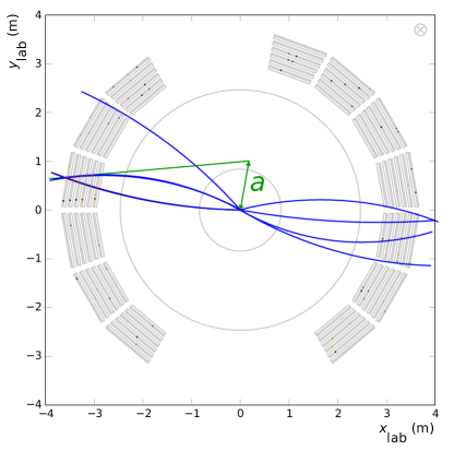
Figure 48: Event display showing the tracks available for the level-1 trigger from the online reconstruction (green) in comparison with helix fits to the contributing tracklets (blue). The offset $a$ from the primary vertex used as measure for $1/p_{\mathrm{T}}$ is shown as well. The colour coding of the tracklets (small boxes) is according to stacks.

Figure 49 shows the timing of the online tracking together with the constraints for the trigger contributions. Between interactions, the FEE is in a sleep mode [78]. In this mode only the ADCs, the digital filters, and the pipeline stages are active. The latter makes it possible to process the data from the full drift time upon arrival of a wake-up signal (see Section 5.1). The processing can be aborted if it is not followed by a level-0 trigger. In this case, a clear sequence is executed for resetting and putting the FEE back to sleep mode. If a level-0 trigger was received, processing continues and the tracklets are sent to the GTU. Here, the track matching and reconstruction runs as the tracklets arrive. The tracks are used to evaluate the trigger conditions (see next sections) until the contribution for the level-1 trigger must be issued to the CTP (about $6\text{\,}\mathrm{\SIUnitSymbolMicro s}$ after the level-0 trigger). The tracking can continue beyond the contribution time for the trigger; the resulting tracks are ignored for the decision but are available for offline analysis (flagged as out-of-time).

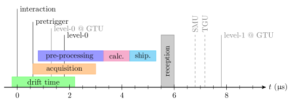
Figure 49: Timing of the various phases for the online tracking with respect to the interaction.

Figure 50 shows the tracking time measured during data taking in p–Pb collisions. It shows the expected linear scaling with the number of tracklets.

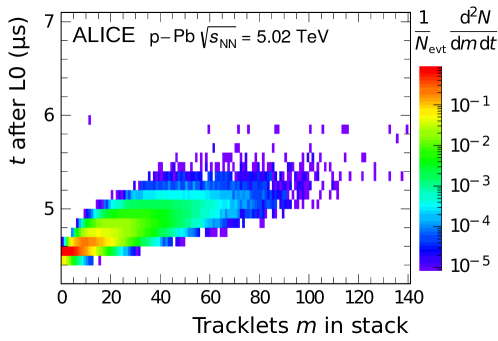
Figure 50: Dependence of the time required for the global online tracking on the tracklet multiplicity in a single stack.

The efficiency of the global online tracking is shown in Fig. 51. In order to separate the efficiency of the online tracking from the acceptance and geometrical limitations, the normalisation is done once for all primary tracks and once for those which are findable, i.e. which have at least 4 tracklets assigned in one stack in the offline tracking (TRD acceptance). The efficiency starts to rise at about 0.6 $\mathrm{GeV}\!/c$, reaches half of its asymptotic value at 1 $\mathrm{GeV}\!/c$, and saturates above about 1.5 $\mathrm{GeV}\!/c$. Lower transverse momenta are not relevant for the trigger operation and corresponding tracks are suppressed at various stages. For comparison, the curve obtained from an ideal Monte Carlo simulation shows slightly higher efficiencies. The difference is caused by non-operational parts of the real detector (see Section 7) not being reflected in the ideal simulation.

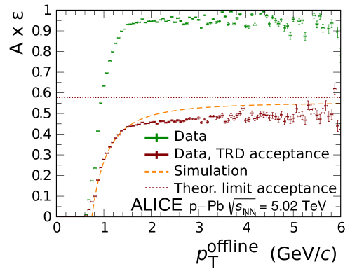
Figure 51: Acceptance times efficiency of the global online tracking for primary tracks (Data) and tracks in the detector acceptance (Data, TRD acceptance) as function of the transverse momentum of the global offline track (trigger threshold at 2–3 $\mathrm{GeV}\!/c$). The results of an ideal simulation, not considering non-operational parts of the real detector, are drawn for comparison. The dotted line shows the theoretical limit of the acceptance with $13$ out of $18$ supermodules installed during the p–Pb data taking period in Run 1.

The correlation of the inverse transverse momentum from online and offline tracking is established by matching global online tracks to global offline tracks, reconstructed with ITS and TPC, based on a geometrical distance measure. An example for pp collisions at $\sqrt{s}=8~{}\mathrm{TeV}$ is shown in Fig. 52. The online estimate correlates well with the offline value in the transverse momentum range relevant for the trigger thresholds, i.e. 2–3 $\mathrm{GeV}\!/c$. The width of the correlation corresponds to an online measured resolution of about 10% for momenta of $1.5-5~{}\mathrm{GeV}\!/c$.

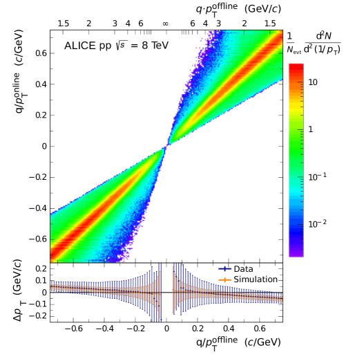
Figure 52: Top: Correlation between $1/p_{\textrm{T}}$ obtained from the online tracking and from a matched offline track for pp collisions at $\sqrt{s}=8~{}\mathrm{TeV}$. Bottom: Difference (points) of the online and offline track $p_{\mathrm{T}}$ for data and simulation. The error bars indicate the corresponding width of the difference in $p_{\textrm{T}}$.

The $p_{\mathrm{T}}$ resolution is crucial for the trigger since it determines the sharpness of the threshold. It is shown in Fig. 53 for a $p_{\mathrm{T}}$ threshold of 3 $\mathrm{GeV}\!/c$, where a width (10–90%) of about 0.6 $\mathrm{GeV}\!/c$ is found. This is also well reproduced by simulations.

As a further development, the online tracking can benefit from taking the chamber alignment into account in the local tracking, and also by enabling the tail cancellation filter in the FEE. This will allow the use of tighter windows for the track matching and, thus, a reduction in combinatorial background while maintaining the same tracking efficiency. This is relevant for the online tracking in the high-multiplicity environment of Pb–Pb collisions. At the time of writing, these improvements are under development.

12.3 Trigger on cosmic-ray muons

Cosmic-ray tracks are used for several purposes in the experiment, e.g. for detector alignment after installation, and before physics runs (see Section 9). Recording sufficient statistics requires a good and clean trigger, in particular for tracks passing the experiment horizontally, for which the rates are very low. Therefore, the first level-1 trigger in ALICE was contributed by the TRD (even before the LHC start-up) in order to select events containing tracks from cosmic rays. It was operated on top of a level-0 trigger from TOF (TOF back-to-back coincidence). At first, when the online tracking was still under commissioning, the selection was based on coincident charge depositions in multiple layers of any stack. Later, it used the full tracking infrastructure with the condition requiring the presence of at least one track in the event. This was sufficient to suppress the background from the impure level-0 input from TOF.

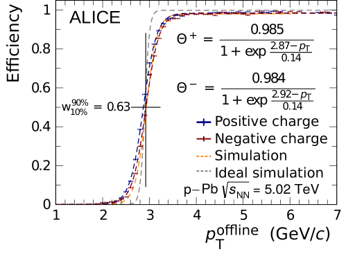
Figure 53: Turn-on curve of the trigger with a $p_{\mathrm{T}}$ threshold of 3 $\mathrm{GeV}\!/c$ for positively and negatively charged particles in comparison to the same variable computed in simulation with a realistic detector geometry (active channels). Also shown is the corresponding distribution for an ideal detector geometry (ideal simulation, not considering misalignment). The onset is characterised by a fit with a Fermi function.

12.4 Trigger on jets

Jets are commonly reconstructed by algorithms which cluster tracks that are close in pseudorapidity and azimuth ($\eta$-$\varphi$ plane). The area covered by a TRD stack roughly corresponds to that of a jet cone of radius $R=0.2$. This allows the presence of several tracks above a $p_{\mathrm{T}}$ threshold within one stack to be used as a signature for a high-$p_{\mathrm{T}}$ jet. The TRD is only sensitive to the charged tracks of the jet, which is also the part that is reconstructed using global offline tracking in the central barrel detectors.

In pp collisions at $\sqrt{s}$ = 8 TeV and p–Pb collisions at $\sqrt{s_{\mathrm{NN}}}$ = 5.02 TeV, the trigger sampled the anticipated integrated luminosity of about 200 nb^-1 and 1.4 nb^-1 in Run 1, respectively. Figure 54 shows the rejection observed in pp collisions ($\sqrt{s}=8~{}\mathrm{TeV}$) for the condition of a certain number of global online tracks above a $p_{\mathrm{T}}$ threshold within any stack. As a compromise between rejection and efficiency for the triggering on jets, 3 tracks above 3 $\mathrm{GeV}\!/c$ were chosen as a trigger condition. This results in a very good rejection, of about $1.5\cdot 10^{-4}$. The jet trigger was also used in p–Pb collisions, where a good performance was achieved as well. However, the higher multiplicity reduces the rejection slightly.

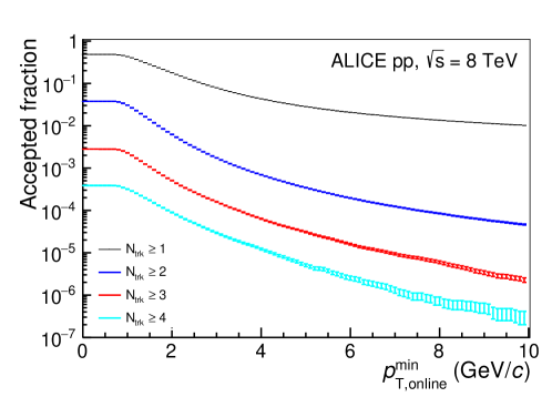
Figure 54: Rejection by the level-1 trigger for requiring 1–4 tracks in any stack ($N_{\rm trk}$) above varying $p_{\mathrm{T}}$ thresholds for pp collisions at $\sqrt{s}$ = 8 TeV [71]. The error bars indicate the statistical uncertainties. The distributions were obtained by counting the number of tracks in a stack above a given threshold and normalised by the number of sampled events.

In Fig. 55 the jet $p_{\mathrm{T}}$ spectra from the TRD-triggered data sample are shown. The jets were reconstructed using the anti-kt jet finder from the Fastjet package [119] with a resolution parameter of $R=0.4$. As expected it extends to significantly larger jet $p_{\mathrm{T}}$ than the one from the minimum-bias data sample. In order to judge the bias on the shape of the spectrum, it is compared to an EMCal-triggered sample. At sufficiently high $p_{\mathrm{T}}$ above about 50 $\mathrm{GeV}\!/c$, the shapes of the spectra agree.

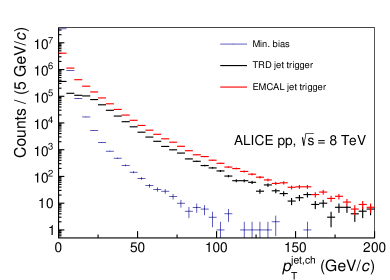
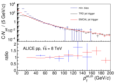
Figure 55: Left: $p_{\mathrm{T}}$ spectra of leading jets for the minimum-bias and triggered samples of pp collisions at $\sqrt{s}$ = 8 TeV [71]. The leading jets are defined as the jets with the highest $p_{\mathrm{T}}$ in the event. Right: For comparison the $p_{\mathrm{T}}$ spectra were scaled to the same yield between 60 and 80 $\mathrm{GeV}\!/c$. The spectra were re-binned to calculate the ratios.

To further judge the bias on the fragmentation, the raw fragmentation function is shown as reconstructed from the jets in the TRD-triggered data sample in Fig. 56. The commonly used variable $\xi$ is defined as

$$\xi=-\log\frac{p_{\mathrm{T}}^{\mathrm{trk}}}{p_{\mathrm{T}}^{\mathrm{jet}}}.$$ (4)

For the lower jet $p_{\mathrm{T}}$ intervals, a clear distortion can be seen at $\xi$ values corresponding to the $p_{\mathrm{T}}$ threshold (in the given jet $p_{\mathrm{T}}$ interval). It disappears for higher jet $p_{\mathrm{T}}$, and agreement with fragmentation functions obtained from an EMCal-triggered sample is found for jet $p_{\mathrm{T}}$ above about 80 $\mathrm{GeV}\!/c$ [71].

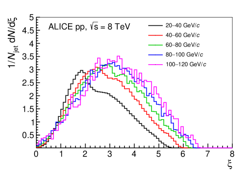
Figure 56: Fragmentation functions of leading jets from the TRD-triggered sample for jets in different $p_{\mathrm{T}}$ intervals in pp collisions at $\sqrt{s}$ = 8 TeV [71]. The leading jets are defined as the jets with the highest $p_{\mathrm{T}}$ in the event.

In order to improve the efficiency of the jet trigger, the counting of tracks can be extended over stack boundaries and, thus, avoid the acceptance gaps introduced between sectors and stacks. Corresponding studies are ongoing.

12.5 Trigger on electrons

During the tracklet reconstruction stage an electron likelihood is assigned to each tracklet allowing for an electron identification (see Section 12.1). It was calculated using a one-dimensional look-up table based on the total accumulated charge (the hardware also allows a two-dimensional LUT). The tracklet length is taken into account as a correction factor applied to the charge, making the actual look-up table universal across the detector. The look-up table is created from reference charge distributions of clean electron and pion samples obtained through topological identification (see Section 11).

In order to select electrons at the trigger level, a combination of a $p_{\mathrm{T}}$ threshold and a PID threshold can be used. The thresholds were optimised for different physics cases. For electrons from semileptonic decays of heavy-flavour hadrons, the goal was to extend the $p_{\mathrm{T}}$ reach at high values. Thus, a $p_{\mathrm{T}}$ threshold of 3 $\mathrm{GeV}\!/c$ was chosen and the PID threshold was adjusted to achieve a rejection of minimum-bias events by a factor of about 100. For the measurement of quarkonia in the electron channel, a $p_{\mathrm{T}}$ threshold of 2 $\mathrm{GeV}\!/c$ was chosen to cover most of the total cross-section. The PID threshold was increased to achieve a similar rejection as for the heavy-flavour trigger. Both triggers were used in pp and p–Pb (and Pb–p) collisions and share a large fraction of the read-out bandwidth. For example in p–Pb collisions at $\sqrt{s_{\mathrm{NN}}}$ = 5.02 TeV recorded during Run 2, about 45% of the events of both electron triggers with late conversion rejection (see below) overlap.

The main background of the electron triggers is caused by the conversion of photons in the detector material at large radii just in front of or at the beginning of the TRD. The emerging electron-positron pairs look like high-$p_{\mathrm{T}}$ tracks and are likely to also be identified as electrons as well. This background is suppressed by requiring (in addition to the thresholds explained above) at least five tracklets, one of which must be in the first layer. The background can be further reduced by requiring that the online track can be matched to a track in the TPC. However, this can not be done during the online tracking, but only during the offline analysis or in the HLT during data taking.

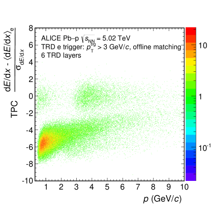
Figure 57: $n_{\sigma^{\mathrm{TPC}}_{\mathrm{e}}}$ as a function of momentum for Pb–p collisions at $\sqrt{s_{\mathrm{NN}}}$ = 5.02 TeV recorded with the electron trigger ($p_{\mathrm{T}}$ threshold at 3 $\mathrm{GeV}\!/c$). Electrons from photon conversions in the detector material were rejected by matching the online track with a track in the TPC.

To judge the performance of the triggers, electron candidates are identified using the signals from TPC, TOF, and TRD. For TPC and TOF the selection is based on $n_{\sigma_{\mathrm{e}}}$, i.e. the deviation of the measured signal from the expected signal normalised to the expected resolution. Figure 57 shows the distribution of this variable for the TPC as a function of the track momentum $p$. The data sample was derived using an electron trigger with a $p_{\mathrm{T}}$ threshold of 3 $\mathrm{GeV}\!/c$ and cleaned in the offline analysis by requiring matching with TPC tracks, i.e. rejecting electrons from photon conversions. Above 3 $\mathrm{GeV}\!/c$ the enhancement of electrons is clearly visible in the region around $n_{\sigma^{\mathrm{TPC}}_{\mathrm{e}}}=0$.

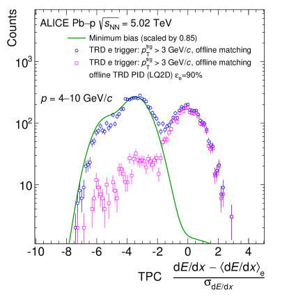
Figure 58: Electron selection for triggered data with and without the TRD offline PID (see Section 11) in Pb–p collisions at $\sqrt{s_{\mathrm{NN}}}$ = 5.02 TeV. Electrons from photon conversions in the detector material were rejected by matching the online track with a track in the TPC. The corresponding distribution for minimum-bias data, scaled to the maximum of the distribution of the triggered data sample, is shown to visualise the TRD trigger capability to enhance electrons.

The enhancement due to the TRD electron trigger in comparison to the minimum-bias trigger is also clearly visible in Fig. 58, which shows a projection of $n_{\sigma^{\mathrm{TPC}}_{\mathrm{e}}}$ in a momentum interval for both data samples. A further suppression of hadrons can be achieved by exploiting the offline PID of the TRD (see Section 11). Figure 59 shows the $p_{\mathrm{T}}$ spectra of electron candidates with 6 layers identified using the TPC and the TOF in the minimum-bias and triggered data sample. The expected onset at the trigger threshold of 3 $\mathrm{GeV}\!/c$ is observed for the triggered events and shows in comparison to the corresponding spectrum from minimum-bias collisions an enhancement of about 700.

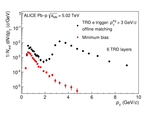
Figure 59: $p_{\mathrm{T}}$ spectra of identified electrons for the minimum-bias and TRD-triggered data sample of Pb–p collisions at $\sqrt{s_{\mathrm{NN}}}$ = 5.02 TeV. For the result of the TRD-triggered sample, electrons from photon conversions in the detector material were rejected by matching the online track with a track in the TPC.

The dominant background for the electron triggers, i.e. the conversion of photons at large radii close to the TRD entrance and in the first part of the TRD, was addressed before RUN 2. The $p_{\mathrm{T}}$ reconstruction in the online tracking assumes tracks originating from the primary vertex, which results in a too-high momentum for the electrons and positrons from ‘late conversions’ as shown in Fig. 60. An online rejection based on the calculation of the sagitta in the read-out chambers was implemented and validated. For a sagitta cut of $\Delta 1/p_{\rm T}=0.2$ $c/\rm{GeV}$ an increased rejection of a factor of 7 at the same efficiency was achieved in pp collisions at $\sqrt{s}$ = 13 TeV [120]. For this selection criterion about 90% of the late conversions are removed, while about 70% of the good tracks are kept. This improvement allows only those tracks to be used for the electron trigger which are not tagged as late conversions. This setting was already successfully used in Run 2.

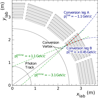
Figure 60: Photon converting into an e⁺ e^- pair at a large radius resembling a high-$p_{\mathrm{T}}$ track for the online tracking (green dashed line) since the offset to the primary vertex is small.

12.6 Trigger on nuclei

A trigger on light nuclei was used for the first time in the high-interaction p–Pb and Pb–p data taking at $\sqrt{s_{\mathrm{NN}}}$ = 5.02 TeV in 2016. It exploits the much higher charge deposition from multiply-charged particles. The trigger enhances mainly the statistics of doubly-charged particles ($Z=2$), i.e. ³He and ⁴He. The trigger was operated with an estimated efficiency of about 30% at a rejection factor of about 600.

This trigger is also used in the pp data taking at 13 TeV during Run 2 to significantly enhance the sample of light nuclei. The trigger does not just enhance the sample of particles with $Z=2$, but also of deuteron, triton and hypertriton (a bound state of a proton, a neutron and a lambda hyperon, which decays weakly into a ³He and a pion) nuclei. This will allow a precise determination of the mass and the lifetime of the latter.

13 Summary

The physics objectives of the TRD together with the challenging LHC environment have led to an ambitious detector design. This required the development of a new chamber design with radiator and electronics. After extensive tests of individual components and the full system, as well as commissioning with cosmic-ray tracks, the detector was ready for data taking with the first collisions provided by the LHC in 2009. During Run 1, the original setup of 7 installed supermodules was further extended, reaching a maximum coverage of 13/18 in azimuth. The detector was completed in the LS 1 before Run 2. Since then it provides coverage of the full azimuthal acceptance of the central barrel. Read-out and trigger components were also upgraded. The developed gas system, services and infrastructure, read-out and electronics, and the Detector Control System allow the successful operation of the detector. The xenon-based gas mixture (over $27\text{\,}{\mathrm{m}}^{3}$) essential for the detection of the TR photons is re-circulated through the detector in order to reduce costs. To minimise the dead time and to cope with the read-out rates for heavy-ion data taking in Run 2, the data from the detector are processed in a highly parallelised read-out tree using a multi-event buffering technique, with link speeds to the DAQ of about 4 Gbit/s. Failsafe and reliable detector operation and its monitoring was achieved. The resulting running efficiencies are about 100% at read-out rates ranging from 100 Hz to 850 Hz in pp and p–Pb collisions, and up to 350 Hz in Pb–Pb collisions.

Robust schemes for calibration, alignment and tracking were established. The TRD adds roughly $70\text{\,}\mathrm{cm}$ to the lever arm of the other tracking detectors in ALICE. The $q/$$p_{\mathrm{T}}$ resolution of high transverse momentum tracks at 40 $\mathrm{GeV}\!/c$ is thus improved by about 40%. In addition, the TRD increases the precision and efficiency of track matching of the detectors that lie behind it. Tracks anchored to the TRD are essential to correct the space charge distortions in the ALICE TPC.

Several hadron and electron identification methods were developed. The electron identification performance is overall better than the design value. At 90% electron efficiency, a pion rejection factor of about 70 is achieved at a momentum of 1 $\mathrm{GeV}\!/c$ for simple identification algorithms. When using the temporal evolution of the signal, a pion rejection factor of up to 410 is obtained.

The complex and efficient design of the trigger allows the provision of triggers based on transverse momentum and electron identification in just about $6\text{\,}\mathrm{\SIUnitSymbolMicro s}$ after the level-0 trigger. This procedure successfully provides enriched samples of high-$p_{\mathrm{T}}$ electrons, light nuclei, and jets in pp and p–Pb collisions. In pp collisions, e.g. at $\sqrt{s}$ = 8 TeV, the jet trigger has efficiently sampled the foreseen integrated luminosity of about 200 nb^-1 during Run 1 with a constant rejection of around $1.5\cdot 10^{-4}$. The TRD will contribute further to the physics output of the experiment in various areas, giving enriched samples of electrons, light nuclei and jets due to the trigger capabilities as well as its contributions to tracking and particle identification.

Appendix A The ALICE Collaboration

S. Acharyaorg137&J. Adamorg96&D. Adamováorg93&C. Adlerorg103&J. Adolfssonorg32&M.M. Aggarwalorg98&G. Aglieri Rinellaorg33&M. Agnelloorg29&N. Agrawalorg46&Z. Ahammedorg137&N. Ahmadorg15&S.U. Ahnorg78&S. Aiolaorg141&A. Akindinovorg63&M. Al-Turanyorg106&S.N. Alamorg137&D. Antonczykorg69&A. Arendorg69&J.L.B. Albaorg111&D.S.D. Albuquerqueorg122&D. Aleksandrovorg89&B. Alessandroorg57&R. Alfaro Molinaorg73&A. Aliciorg11^,org25^,org52&A. Alkinorg3&J. Almeorg20&T. Altorg69&L. Altenkamperorg20&I. Altsybeevorg136&C. Alves Garcia Pradoorg121&C. Andreiorg86&D. Andreouorg33&H.A. Andrewsorg110&A. Andronicorg106&V. Anguelovorg103&C. Ansonorg96&T. Antičićorg107&F. Antinoriorg55&P. Antonioliorg52&R. Anwarorg124&L. Aphecetcheorg114&H. Appelshäuserorg69&S. Arcelliorg25&R. Arnaldiorg57&O.W. Arnoldorg104^,org34&I.C. Arseneorg19&M. Arslandokorg103&B. Audurierorg114&A. Augustinusorg33&R. Averbeckorg106&M.D. Azmiorg15&A. Badalàorg54&Y.W. Baekorg59^,org77&S. Bagnascoorg57&R. Bailhacheorg69&R. Balaorg100&A. Baldisseriorg74&M. Ballorg43&R.C. Baralorg66&A.M. Barbanoorg24&R. Barberaorg26&F. Barileorg31^,org51&L. Barioglioorg24&G.G. Barnaföldiorg140&L.S. Barnbyorg92&V. Barretorg131&P. Bartaliniorg7&K. Barthorg33&D. Bartosorg86&E. Bartschorg69&M. Basileorg25&N. Bastidorg131&S. Basuorg139&B. Bathenorg70&G. Batigneorg114&B. Batyunyaorg76&P.C. Batzingorg19&C. Baumannorg69&I.G. Beardenorg90&H. Beckorg103&C. Beddaorg62&N.K. Beheraorg59&I. Belikovorg133&F. Belliniorg25^,org33&H. Bello Martinezorg2&R. Bellwiedorg124&L.G.E. Beltranorg120&V. Belyaevorg82&G. Bencediorg140&S. Beoleorg24&I. Berceanuorg86&A. Bercuciorg86&Y. Berdnikovorg95&D. Berenyiorg140&R.A. Bertensorg127&D. Berzanoorg33&L. Betevorg33&A. Bhasinorg100&I.R. Bhatorg100&A.K. Bhatiorg98&B. Bhattacharjeeorg42&J. Bhomorg118&A. Bianchiorg24&L. Bianchiorg124&N. Bianchiorg49&C. Bianchinorg139&J. Bielčíkorg37&J. Bielčíkováorg93&A. Bilandzicorg104^,org34&G. Biroorg140&R. Biswasorg4&S. Biswasorg4&J.T. Blairorg119&D. Blauorg89&C. Blumeorg69&G. Bocaorg134&F. Bockorg81^,org33^,org103&A. Bogdanovorg82&L. Boldizsárorg140&M. Bombaraorg38&G. Bonomiorg135&M. Bonoraorg33&J. Bookorg69&H. Borelorg74&A. Borissovorg17&M. Borriorg126&E. Bottaorg24&C. Bourjauorg90&L. Bratrudorg69&P. Braun-Munzingerorg106&M. Bregantorg121&T.A. Brokerorg69&M. Brozorg37&E.J. Bruckenorg44&E. Brunaorg57&G.E. Brunoorg31&D. Bucherorg70&D. Budnikovorg108&H. Bueschingorg69&S. Bufalinoorg29&P. Buhlerorg113&P. Buncicorg33&O. Buschorg130&Z. Butheleziorg75&J.B. Buttorg14&J.T. Buxtonorg16&J. Cabalaorg116&D. Caffarriorg33^,org91&H. Cainesorg141&A. Calivaorg62&E. Calvo Villarorg111&P. Cameriniorg23&A.A. Caponorg113&G. Caragheorgheopolorg86&F. Carenaorg33&W. Carenaorg33&F. Carnesecchiorg25^,org11&J. Castillo Castellanosorg74&A.J. Castroorg127&E.A.R. Casulaorg53&V. Catanescuorg86&C. Ceballos Sanchezorg9&P. Cerelloorg57&S. Chandraorg137&B. Changorg125&S. Chapelandorg33&M. Chartierorg126&S. Chattopadhyayorg137&S. Chattopadhyayorg109&A. Chauvinorg34^,org104&S. Chernenkoorg76&M. Cherneyorg96&C. Cheshkovorg132&B. Cheynisorg132&V. Chibante Barrosoorg33&D.D. Chinellatoorg122&S. Choorg59&P. Chochulaorg33&M. Chojnackiorg90&S. Choudhuryorg137&T. Chowdhuryorg131&P. Christakoglouorg91&C.H. Christensenorg90&P. Christiansenorg32&T. Chujoorg130&S.U. Chungorg17&C. Cicaloorg53&L. Cifarelliorg11^,org25&F. Cindoloorg52&M. Ciobanuorg86&J. Cleymansorg99&F. Colamariaorg31&D. Colellaorg33^,org51^,org64&A. Colluorg81&M. Colocciorg25&M. Concasorg57orgI&G. Conesa Balbastreorg80&Z. Conesa del Valleorg60&M.E. Connorsorg141orgII&J.G. Contrerasorg37&T.M. Cormierorg94&Y. Corrales Moralesorg57&I. Cortés Maldonadoorg2&P. Corteseorg30&M.R. Cosentinoorg123&F. Costaorg33&S. Costanzaorg134&J. Crkovskáorg60&P. Crochetorg131&E. Cuautleorg71&L. Cunqueiroorg70&T. Dahmsorg34^,org104&A. Daineseorg55&M.C. Danischorg103&A. Danuorg67&D. Dasorg109&I. Dasorg109&S. Dasorg4&A. Dashorg87&S. Dashorg46&H. Dauesorg106&S. Deorg121^,org47&A. De Caroorg28&G. de Cataldoorg51&C. de Contiorg121&J. de CuvelandorgIII&A. De Falcoorg22&D. De Gruttolaorg28^,org11&N. De Marcoorg57&S. De Pasqualeorg28&R.D. De Souzaorg122&H.F. Degenhardtorg121&A. Deistingorg106^,org103&A. Delofforg85&C. Deplanoorg91&A. Devismesorg106&P. Dhankherorg46&D. Di Bariorg31&A. Di Mauroorg33&P. Di Nezzaorg49&B. Di Ruzzaorg55&T. Dietelorg99&P. Dillensegerorg69&R. Diviàorg33&Ø. Djuvslandorg20&A. Dobrinorg33&D. Domenicis Gimenezorg121&B. Dönigusorg69&O. Dordicorg19&L.V.V. Doremalenorg62&A.K. Dubeyorg137&A. Dublaorg106&L. Ducrouxorg132&A.K. Duggalorg98&P. Dupieuxorg131&V. Dutaorg86&R.J. Ehlersorg141&D. Eliaorg51&D. Emschermannorg103&E. Endressorg111&H. Engelorg68&E. Eppleorg141&B. Erazmusorg114&F. Erhardtorg97&B. Espagnonorg60&S. Esumiorg130&G. Eulisseorg33&J. Eumorg17&D. Evansorg110&S. Evdokimovorg112&L. Fabbiettiorg104^,org34&J. Faivreorg80&A. Fantoniorg49&M. Faselorg94^,org81&O. Fateevorg76&L. Feldkamporg70&A. Felicielloorg57&G. Feofilovorg136&J. Ferenceiorg93&A. Fernández Téllezorg2&A. Ferrettiorg24&A. Festantiorg33^,org27&V.J.G. Feuillardorg131^,org74&J. Figielorg118&M.A.S. Figueredoorg121&S. Filchaginorg108&D. Finogeevorg61&F.M. Fiondaorg20^,org22&M. Fleckorg103&M. Florisorg33&S. Foertschorg75&P. Fokaorg106&S. Fokinorg89&E. Fragiacomoorg58&A. Francesconorg33&A. Franciscoorg114&U. Frankenfeldorg106&S. Freuenorg103&G.G. Fronzeorg24&U. Fuchsorg33&C. Furgetorg80&A. Fursorg61&M. Fusco Girardorg28&J.J. Gaardhøjeorg90&M. Gagliardiorg24&A.M. Gagoorg111&K. Gajdosovaorg90&M. Gallioorg24&C.D. Galvanorg120&P. Ganotiorg84&C. Garabatosorg106&E. Garcia-Solisorg12&K. Gargorg26&C. Gargiuloorg33&P. Gasikorg34^,org104&H. Gatzorg70&E.F. Gaugerorg119&M.B. Gay Ducatiorg72&M. Germainorg114&J. Ghoshorg109&P. Ghoshorg137&S.K. Ghoshorg4&P. Gianottiorg49&G. Gioluorg86&P. Giubellinoorg106^,org57^,org33&P. Giubilatoorg27&E. Gladysz-Dziadusorg118&R. Glasoworg70org*&P. Glässelorg103&S. Gremmlerorg70&D.M. Goméz Coralorg73&A. Gomez Ramirezorg68&A.S. Gonzalezorg33&S. Gorbunovorg40&L. Görlichorg118&S. Gotovacorg117&D. Gottschalkorg103&H. Gottschlagorg70&V. Grabskiorg73&L.K. Graczykowskiorg138&K.L. Grahamorg110&R. Grajcarekorg103&L. Greinerorg81&A. Grelliorg62&C. Grigorasorg33&V. Grigorievorg82&A. Grigoryanorg1&S. Grigoryanorg76&H. Grimmorg70&N. Grionorg58&J.M. Gronefeldorg106&F. Grosaorg29&J.F. Grosse-Oetringhausorg33&R. Grossoorg106&L. Gruberorg113&F. Guberorg61&R. Guernaneorg80&B. Guerzoniorg25&K. Gulbrandsenorg90&T. Gunjiorg129&A. Guptaorg100&R. Guptaorg100&M. Gutfleischorg106&I.B. Guzmanorg2&R. Haakeorg33&C. Hadjidakisorg60&H. Hamagakiorg83&G. Hamarorg140&J.C. Hamonorg133&M.R. Haqueorg62&J.W. Harrisorg141&M. Hartigorg69&A. Hartonorg12&H. Hassanorg80&D. Hatzifotiadouorg11^,org52&S. Hayashiorg129&S.T. Heckelorg69&J. Hehnerorg106&M. Heideorg70&E. Hellbärorg69&H. Helstruporg35&A. Herghelegiuorg86&G. Herrera Corralorg10&F. Herrmannorg70&N. Herrmannorg103&B.A. Hessorg102&K.F. Hetlandorg35&H. Hillemannsorg33&C. Hillsorg126&B. Hippolyteorg133&J. Hladkyorg65&B. Hohlwegerorg104&D. Horakorg37&S. Hornungorg106&R. Hosokawaorg130^,org80&P. Hristovorg33&S. Huberorg106&C. Hughesorg127&T.J. Humanicorg16&N. Hussainorg42&T. Hussainorg15&D. Hutterorg40&D.S. Hwangorg18&S.A. Iga Buitronorg71&R. Ilkaevorg108&M. Inabaorg130&M. Ippolitovorg82^,org89&M. Irfanorg15&M.S. Islamorg109&M. Ivanovorg106&V. Ivanovorg95&V. Izucheevorg112&B. Jacakorg81&N. Jacazioorg25&P.M. Jacobsorg81&M.B. Jadhavorg46&J. Jadlovskyorg116&S. Jaelaniorg62&C. Jahnkeorg34&M.J. Jakubowskaorg138&M.A. Janikorg138&P.H.S.Y. Jayarathnaorg124&C. Jenaorg87&S. Jenaorg124&M. Jercicorg97&R.T. Jimenez Bustamanteorg106&P.G. Jonesorg110&A. Juskoorg110&P. Kalinakorg64&A. Kalweitorg33&J.H. Kangorg142&V. Kaplinorg82&S. Karorg137&A. Karasu Uysalorg79&O. Karavichevorg61&T. Karavichevaorg61&L. Karayanorg106^,org103&P. Karczmarczykorg33&E. Karpechevorg61&U. Kebschullorg68&R. Keidelorg143&D.L.D. Keijdenerorg62&M. Keilorg33&B. Ketzerorg43&Z. Khabanovaorg91&P. Khanorg109&S.A. Khanorg137&A. Khanzadeevorg95&Y. Kharlovorg112&A. Khatunorg15&A. Khuntiaorg47&M.M. Kielbowiczorg118&B. Kilengorg35&B. Kimorg130&D. Kimorg142&D.J. Kimorg125&H. Kimorg142&J.S. Kimorg41&J. Kimorg103&M. Kimorg59&M. Kimorg142&S. Kimorg18&T. Kimorg142&S. Kirschorg40&I. Kiselorg40&S. Kiselevorg63&A. Kisielorg138&E. Kislovorg76&G. Kissorg140&J.L. Klayorg6&C. Kleinorg69&J. Kleinorg33&C. Klein-Bösingorg70&M. Klein-Bösingorg70&M. Kliemantorg69&H. Klingenmeyerorg103&S. Klewinorg103&A. Klugeorg33&M.L. Knichelorg33^,org103&A.G. Knospeorg124&C. Kobdajorg115&M. Kofaragoorg140&M. Kohnorg70&T. Kolleggerorg106&V. Kondratievorg136&N. Kondratyevaorg82&E. Kondratyukorg112&A. Konevskikhorg61&M. Konnoorg130&M. Konyushikhinorg139&M. Kopcikorg116&M. Kourorg100&C. Kouzinopoulosorg33&O. Kovalenkoorg85&V. Kovalenkoorg136&M. Kowalskiorg118&G. Koyithatta Meethaleveeduorg46&I. Králikorg64&F. Kramerorg69&A. Kravčákováorg38&T. KrawutschkeorgIV&L. Kreisorg106&M. Krivdaorg64^,org110&F. Krizekorg93&D. Krumbhornorg103&E. Kryshenorg95&M. Krzewickiorg40&A.M. Kuberaorg16&V. Kučeraorg93&C. Kuhnorg133&P.G. Kuijerorg91&A. Kumarorg100&J. Kumarorg46&L. Kumarorg98&S. Kumarorg46&S. Kunduorg87&P. Kurashviliorg85&A. Kurepinorg61&A.B. Kurepinorg61&A. Kuryakinorg108&S. Kushpilorg93&M.J. Kweonorg59&Y. Kwonorg142&S.L. La Pointeorg40&P. La Roccaorg26&C. Lagana Fernandesorg121&Y.S. Laiorg81&I. Lakomovorg33&R. Langoyorg39&K. Lapidusorg141&C. Laraorg68&A. Lardeuxorg19^,org74&A. Lattucaorg24&E. Laudiorg33&R. Lavickaorg37&R. Leaorg23&L. Leardiniorg103&S. Leeorg142&F. Lehasorg91&T. Lehmannorg103&J. Lehnerorg69&S. Lehnerorg113&J. Lehrbachorg40&R.C. Lemmonorg92&V. Lentiorg51&E. Leograndeorg62&I. León Monzónorg120&F. LesserorgIII&P. Lévaiorg140&X. Liorg13&J. Lienorg39&R. Lietavaorg110&B. Limorg17&S. Lindalorg19&V. Lindenstruthorg40&S.W. Lindsayorg126&C. Lippmannorg106&M.A. Lisaorg16&V. Litichevskyiorg44&W.J. Llopeorg139&D.F. Lodatoorg62&D. Lohnerorg103&P.I. Loenneorg20&V. Loginovorg82&C. Loizidesorg81&P. Loncarorg117&X. Lopezorg131&E. López Torresorg9&A. Loweorg140&X. Luorg103&W. Ludolphsorg103&P. Luettigorg69&J.R. Luhderorg70&M. Lunardonorg27&G. Luparelloorg58^,org23&M. Lupiorg33&T.H. Lutzorg141&A. Maevskayaorg61&M. Magerorg33&C. Magureanuorg86&S. Mahajanorg100&T. Mahmoudorg103&S.M. Mahmoodorg19&A. Maireorg133&R.D. Majkaorg141&M. Malaevorg95&L. Malininaorg76orgV&D. Mal’Kevichorg63&P. Malzacherorg106&A. Mamonovorg108&V. Mankoorg89&F. Mansoorg131&V. Manzariorg51&Y. Maoorg7&M. Marchisoneorg75^,org128&J. Marešorg65&G.V. Margagliottiorg23&A. Margottiorg52&J. Marguttiorg62&A. Marínorg106&C. Markertorg119&M. Marquardorg69&N.A. Martinorg106&P. Martinengoorg33&J.A.L. Martinezorg68&M.I. Martínezorg2&G. Martínez Garcíaorg114&M. Martinez Pedreiraorg33&S. Masciocchiorg106&M. Maseraorg24&A. Masoniorg53&E. Massonorg114&A. Mastroserioorg51&A.M. Mathisorg34^,org104&A. Matyjaorg127&C. Mayerorg118&J. Mazerorg127&M. Mazzilliorg31&M.A. Mazzoniorg56&F. Meddiorg21&Y. Melikyanorg82&A. Menchaca-Rochaorg73&E. Meninnoorg28&J. Mercado Pérezorg103&M. Meresorg36&S. Mhlangaorg99&Y. Miakeorg130&M.M. Mieskolainenorg44&D.L. Mihaylovorg104&K. Mikhaylovorg63^,org76&J. Milosevicorg19&A. Mischkeorg62&A.N. Mishraorg47&D. Miśkowiecorg106&J. Mitraorg137&C.M. Mituorg67&N. Mohammadiorg62&B. Mohantyorg87&M. Mohisin Khanorg15orgVI&D.A. Moreira De Godoyorg70&L.A.P. Morenoorg2&S. Morettoorg27&Y. Morinoorg129&A. Morrealeorg114&A. Morschorg33&V. Mucciforaorg49&E. Mudnicorg117&D. Mühlheimorg70&S. Muhuriorg137&M. Mukherjeeorg4&J.D. Mulliganorg141&M.G. Munhozorg121&K. Münningorg43&R.H. Munzerorg69&H. Murakamiorg129&S. Murrayorg75&L. Musaorg33&J. Musinskyorg64&C.J. Myersorg124&J.W. Myrchaorg138&J. Mückeorg103&D. Nagorg4&B. Naikorg46&R. Nairorg85&B.K. Nandiorg46&R. Naniaorg11^,org52&E. Nappiorg51&A. Narayanorg46&M.U. Naruorg14&H. Natal da Luzorg121&C. Nattrassorg127&S.R. Navarroorg2&K. Nayakorg87&R. Nayakorg46&T.K. Nayakorg137&S. Nazarenkoorg108&A. Nedosekinorg63&R.A. Negrao De Oliveiraorg33&M. Neherorg103&L. Nellenorg71&S.V. Nesboorg35&F. Ngorg124&M. Nicassioorg106&M. Niculescuorg67&J. Niedzielaorg33^,org138&B.S. Nielsenorg90&S. Nikolaevorg89&S. Nikulinorg89&V. Nikulinorg95&F. Noferiniorg52^,org11&P. Nomokonovorg76&G. Noorenorg62&J.C.C. Norisorg2&J. Normanorg126&A. Nyaninorg89&J. Nystrandorg20&H. Oeschlerorg103org*&S. Ohorg141&A. Ohlsonorg33^,org103&T. Okuboorg45&L. Olahorg140&J. Oleniaczorg138&A.C. Oliveira Da Silvaorg121&M.H. Oliverorg141&J. Onderwaaterorg106&C. Oppedisanoorg57&R. Oravaorg44&M. Oravecorg116&A. Ortiz Velasquezorg71&A. Oskarssonorg32&J. Otwinowskiorg118&K. Oyamaorg83&Y. Pachmayerorg103&V. Pacikorg90&D. Paganoorg135&P. Paganoorg28&G. Paićorg71&Y. Panebratsevorg76&P. Palniorg7&J. Panorg139&A.K. Pandeyorg46&S. Panebiancoorg74&V. Papikyanorg1&G.S. Pappalardoorg54&P. Pareekorg47&J. Parkorg59&W. Parkorg106&S. Parmarorg98&A. Passfeldorg70&S.P. Pathakorg124&R.N. Patraorg137&B. Paulorg57&H. Peiorg7&T. Peitzmannorg62&X. Pengorg7&L.G. Pereiraorg72&H. Pereira Da Costaorg74&D. Peresunkoorg89^,org82&E. Perez Lezamaorg69&V. Peskovorg69&Y. Pestovorg5&V. Petráčekorg37&M. Petrisorg86&V. Petrovorg112&M. Petroviciorg86&C. Pettaorg26&R.P. Pezziorg72&S. Pianoorg58&M. Piknaorg36&P. Pillotorg114&L.O.D.L. Pimentelorg90&O. Pinazzaorg52^,org33&L. Pinskyorg124&N. Pitzorg69&D.B. Piyarathnaorg124&M. Płoskońorg81&M. Planinicorg97&F. Pliquettorg69&J. Plutaorg138&S. Pochybovaorg140&P.L.M. Podesta-Lermaorg120&M.G. Poghosyanorg94&B. Polichtchoukorg112&N. Poljakorg97&W. Poonsawatorg115&A. Poporg86&H. Poppenborgorg70&S. Porteboeuf-Houssaisorg131&V. Pozdniakovorg76&S.K. Prasadorg4&R. Preghenellaorg52&F. Prinoorg57&C.A. Pruneauorg139&I. Pshenichnovorg61&M. Puccioorg24&G. Pudduorg22&P. Pujahariorg139&V. Puninorg108&J. Putschkeorg139&S. Radomskiorg103&A. Rachevskiorg58&S. Rahaorg4&S. Rajputorg100&J. Rakorg125&A. Rakotozafindrabeorg74&L. Ramelloorg30&F. Ramiorg133&D.B. Ranaorg124&R. Raniwalaorg101&S. Raniwalaorg101&S.S. Räsänenorg44&B.T. Rascanuorg69&D. Ratheeorg98&V. Ratzaorg43&I. Ravasengaorg29&K.F. Readorg94^,org127&K. Redlichorg85orgVII&A. Rehmanorg20&P. Reicheltorg69&F. Reidtorg33&A. Reischlorg103&X. Renorg7&R. Renfordtorg69&A.R. Reolonorg49&A. Reshetinorg61&K. Reygersorg103&V. Riabovorg95&R.A. Ricciorg50&T. Richertorg62&M. Richterorg19&P. Riedlerorg33&W. Rieglerorg33&F. Riggiorg26&C. Risteaorg67&M. Rodríguez Cahuantziorg2&K. Røedorg19&E. Rogochayaorg76&D. Rohrorg40^,org33&D. Röhrichorg20&P.S. Rokitaorg138&F. Ronchettiorg49&E.D. Rosasorg71&P. Rosnetorg131&A. Rossiorg27^,org55&A. Rotondiorg134&F. Roukoutakisorg84&A. Royorg47&C. Royorg133&P. Royorg109&O.V. Ruedaorg71&R. Ruiorg23&B. Rumyantsevorg76&I. Rusanovorg103&A. Rustamovorg88&E. Ryabinkinorg89&Y. Ryabovorg95&A. Rybickiorg118&S. Saarinenorg44&S. Sadhuorg137&S. Sadovskyorg112&K. Šafaříkorg33&S.K. Sahaorg137&B. Sahlmullerorg69&B. Sahooorg46&P. Sahooorg47&R. Sahooorg47&S. Sahooorg66&P.K. Sahuorg66&J. Sainiorg137&S. Sakaiorg130&D. Sakataorg130&M.A. Salehorg139&J. Salzwedelorg16&S. Sambyalorg100&V. Samsonovorg95^,org82&A. Sandovalorg73&H. Sannorg106org*&M. Sanoorg130&R. Santoorg70&D. Sarkarorg137&N. Sarkarorg137&P. Sarmaorg42&M.H.P. Sasorg62&E. Scapparoneorg52&F. Scarlassaraorg27&B. Schaeferorg94&R.P. Scharenbergorg105&H.S. Scheidorg69&C. Schiauaorg86&R. Schickerorg103&C. Schmidtorg106&H.R. Schmidtorg102&M.O. Schmidtorg103&M. Schmidtorg102&N.V. Schmidtorg94^,org69&S. Schmiedererorg103&R. SchneiderorgIII&J. Schukraftorg33&R. Schulzeorg106&Y. Schutzorg33^,org133^,org114&K. Schwarzorg106&K. Schwedaorg106&G. Scioliorg25&E. Scomparinorg57&R. Scottorg127&S. Sedykhorg106&M. Šefčíkorg38&J.E. Segerorg96&Y. Sekiguchiorg129&D. Sekihataorg45&I. Selyuzhenkovorg82^,org106&K. Senosiorg75&S. Senyukovorg33^,org133^,org3&E. Serradillaorg73&P. Settorg46&A. Sevcencoorg67&A. Shabanovorg61&A. Shabetaiorg114&R. Shahoyanorg33&W. Shaikhorg109&A. Shangaraevorg112&A. Sharmaorg98&A. Sharmaorg100&M. Sharmaorg100&M. Sharmaorg100&N. Sharmaorg98^,org127&A.I. Sheikhorg137&K. Shigakiorg45&S. Shimanskyorg76&Q. Shouorg7&K. Shtejerorg24^,org9&P. Shuklaorg103&Y. Sibiriakorg89&E. Sickingorg70&S. Siddhantaorg53&K.M. Sielewiczorg33&T. Siemiarczukorg85&S. Silaevaorg89&D. Silvermyrorg32&C. Silvestreorg80&G. Simatovicorg97&R. Simonorg106&G. Simonettiorg33&R. Singarajuorg137&R. Singhorg87&V. Singhalorg137&T. Sinhaorg109&B. Sitarorg36&M. Sittaorg30&T.B. Skaaliorg19&M. Slupeckiorg125&N. Smirnovorg141&L. Smykovorg76&R.J.M. Snellingsorg62&T.W. Snellmanorg125&H. Solveitorg103&W. Sommerorg69&J. Songorg17&M. Songorg142&F. Soramelorg27&S. Sorensenorg127&F. Sozziorg106&E. Spiritiorg49&I. Sputowskaorg118&B.K. Srivastavaorg105&J. Stachelorg103&I. Stanorg67&P. Stankusorg94&H. Stelzerorg106&E. Stenlundorg32&J. Stillerorg103&D. Stoccoorg114&M. Stockmeyerorg103&M.M. Storetvedtorg35&P. Strmenorg36&A.A.P. Suaideorg121&T. Sugitateorg45&C. Suireorg60&M. Suleymanovorg14&M. Suljicorg23&R. Sultanovorg63&M. Šumberaorg93&S. Sumowidagdoorg48&K. Suzukiorg113&S. Swainorg66&A. Szaboorg36&I. Szarkaorg36&U. Tabassamorg14&J. Takahashiorg122&G.J. Tambaveorg20&N. Tanakaorg130&M. Tarhiniorg60&M. Tariqorg15&M.G. Tarzilaorg86&A. Tauroorg33&G. Tejeda Muñozorg2&A. Telescaorg33&K. Terasakiorg129&C. Terrevoliorg27&B. Teyssierorg132&D. Thakurorg47&S. Thakurorg137&D. Thomasorg119&F. Thoresenorg90&R. Tieulentorg132&A. Tikhonovorg61&H. Tilsnerorg103&A.R. Timminsorg124&A. Toiaorg69&S.R. Torresorg120&S. Tripathyorg47&S. Trogoloorg24&G. Trombettaorg31&L. Tropporg38&V. Trubnikovorg3&W.H. Trzaskaorg125&B.A. Trzeciakorg62&G. Tsiledakisorg103&T. Tsujiorg129&A. Tumkinorg108&R. Turrisiorg55&T.S. Tveterorg19&K. Ullalandorg20&E.N. Umakaorg124&A. Urasorg132&G.L. Usaiorg22&A. Utrobicicorg97&M. Valaorg116^,org64&J. Van Der Maarelorg62&J.W. Van Hoorneorg33&M. van Leeuwenorg62&T. Vanatorg93&H. Vargasorg69&P. Vande Vyvreorg33&D. Vargaorg140&A. Vargasorg2&M. Vargyasorg125&R. Varmaorg46&M. Vasileiouorg84&A. Vasilievorg89&A. Vauthierorg80&O. Vázquez Doceorg104^,org34&V. Vecherninorg136&A.M. Veenorg62&A. Velureorg20&E. Vercellinorg24&S. Vergara Limónorg2&R. Vernetorg8&R. Vértesiorg140&L. Vickovicorg117&S. Vigoloorg62&J. Viinikainenorg125&Z. Vilakaziorg128&O. Villalobos Baillieorg110&A. Villatoro Telloorg2&A. Vinogradovorg89&L. Vinogradovorg136&T. Virgiliorg28&V. Vislaviciusorg32&A. Vodopyanovorg76&M.A. Völklorg103^,org102&K. Voloshinorg63&S.A. Voloshinorg139&G. Volpeorg31&B. von Hallerorg33&I. Vorobyevorg104^,org34&D. Voscekorg116&D. Vranicorg33^,org106&J. Vrlákováorg38&B. Vulpescuorg103&B. Wagnerorg20&H. Wangorg62&M. Wangorg7&Y. Wangorg103&D. Watanabeorg130&K. Watanabeorg130&Y. Watanabeorg129^,org130&M. Weberorg113&S.G. Weberorg106&D. Wegerleorg69&D.F. Weiserorg103&S.C. Wenzelorg33&J.P. Wesselsorg70&U. Westerhofforg70&A.M. Whiteheadorg99&J. Wiechulaorg69&J. Wikneorg19&A. Wilkorg70&G. Wilkorg85&J. Wilkinsonorg103^,org52&G.A. Willemsorg70&M.C.S. Williamsorg52&E. Willsherorg110&B. Windelbandorg103&M. Winnorg103&W.E. Wittorg127&C. Xuorg103&S. Yalcinorg79&K. Yamakawaorg45&P. Yangorg7&S. Yanoorg45&Z. Yinorg7&H. Yokoyamaorg130^,org80&I.-K. Yooorg17&J.H. Yoonorg59&V. Yurchenkoorg3&V. Yurevichorg76&V. Zaccoloorg57&A. Zamanorg14&C. Zampolliorg33&H.J.C. Zanoliorg121&Y. Zanevskiorg76org*&N. Zardoshtiorg110&A. Zarochentsevorg136&P. Závadaorg65&N. Zaviyalovorg108&H. Zbroszczykorg138&M. Zhalovorg95&H. Zhangorg20^,org7&X. Zhangorg7&Y. Zhangorg7&C. Zhangorg62&Z. Zhangorg131^,org7&C. Zhaoorg19&N. Zhigarevaorg63&D. Zhouorg7&Y. Zhouorg90&Z. Zhouorg20&H. Zhuorg20&J. Zhuorg7&A. Zichichiorg11^,org25&S. Zimmerorg103&A. Zimmermannorg103&M.B. Zimmermannorg33&G. Zinovjevorg3&J. Zmeskalorg113&S. Zouorg7&

Affiliation notes

org*Deceased

orgIDipartimento DET del Politecnico di Torino, Turin, Italy

orgIIGeorgia State University, Atlanta, Georgia, United States

orgIIIKirchhoff-Institut für Physik, Ruprecht-Karls-Universität Heidelberg, Heidelberg, Germany

orgIVFachhochschule Köln, Köln, Germany

orgVM.V. Lomonosov Moscow State University, D.V. Skobeltsyn Institute of Nuclear, Physics, Moscow, Russia

orgVIDepartment of Applied Physics, Aligarh Muslim University, Aligarh, India

orgVIIInstitute of Theoretical Physics, University of Wroclaw, Poland

Collaboration Institutes

org1A.I. Alikhanyan National Science Laboratory (Yerevan Physics Institute) Foundation, Yerevan, Armenia

org2Benemérita Universidad Autónoma de Puebla, Puebla, Mexico

org3Bogolyubov Institute for Theoretical Physics, Kiev, Ukraine

org4Bose Institute, Department of Physics and Centre for Astroparticle Physics and Space Science (CAPSS), Kolkata, India

org5Budker Institute for Nuclear Physics, Novosibirsk, Russia

org6California Polytechnic State University, San Luis Obispo, California, United States

org7Central China Normal University, Wuhan, China

org8Centre de Calcul de l’IN2P3, Villeurbanne, Lyon, France

org9Centro de Aplicaciones Tecnológicas y Desarrollo Nuclear (CEADEN), Havana, Cuba

org10Centro de Investigación y de Estudios Avanzados (CINVESTAV), Mexico City and Mérida, Mexico

org11Centro Fermi - Museo Storico della Fisica e Centro Studi e Ricerche “Enrico Fermi’, Rome, Italy

org12Chicago State University, Chicago, Illinois, United States

org13China Institute of Atomic Energy, Beijing, China

org14COMSATS Institute of Information Technology (CIIT), Islamabad, Pakistan

org15Department of Physics, Aligarh Muslim University, Aligarh, India

org16Department of Physics, Ohio State University, Columbus, Ohio, United States

org17Department of Physics, Pusan National University, Pusan, Republic of Korea

org18Department of Physics, Sejong University, Seoul, Republic of Korea

org19Department of Physics, University of Oslo, Oslo, Norway

org20Department of Physics and Technology, University of Bergen, Bergen, Norway

org21Dipartimento di Fisica dell’Università ’La Sapienza’ and Sezione INFN, Rome, Italy

org22Dipartimento di Fisica dell’Università and Sezione INFN, Cagliari, Italy

org23Dipartimento di Fisica dell’Università and Sezione INFN, Trieste, Italy

org24Dipartimento di Fisica dell’Università and Sezione INFN, Turin, Italy

org25Dipartimento di Fisica e Astronomia dell’Università and Sezione INFN, Bologna, Italy

org26Dipartimento di Fisica e Astronomia dell’Università and Sezione INFN, Catania, Italy

org27Dipartimento di Fisica e Astronomia dell’Università and Sezione INFN, Padova, Italy

org28Dipartimento di Fisica ‘E.R. Caianiello’ dell’Università and Gruppo Collegato INFN, Salerno, Italy

org29Dipartimento DISAT del Politecnico and Sezione INFN, Turin, Italy

org30Dipartimento di Scienze e Innovazione Tecnologica dell’Università del Piemonte Orientale and INFN Sezione di Torino, Alessandria, Italy

org31Dipartimento Interateneo di Fisica ‘M. Merlin’ and Sezione INFN, Bari, Italy

org32Division of Experimental High Energy Physics, University of Lund, Lund, Sweden

org33European Organization for Nuclear Research (CERN), Geneva, Switzerland

org34Excellence Cluster Universe, Technische Universität München, Munich, Germany

org35Faculty of Engineering, Bergen University College, Bergen, Norway

org36Faculty of Mathematics, Physics and Informatics, Comenius University, Bratislava, Slovakia

org37Faculty of Nuclear Sciences and Physical Engineering, Czech Technical University in Prague, Prague, Czech Republic

org38Faculty of Science, P.J. Šafárik University, Košice, Slovakia

org39Faculty of Technology, Buskerud and Vestfold University College, Tonsberg, Norway

org40Frankfurt Institute for Advanced Studies, Johann Wolfgang Goethe-Universität Frankfurt, Frankfurt, Germany

org41Gangneung-Wonju National University, Gangneung, Republic of Korea

org42Gauhati University, Department of Physics, Guwahati, India

org43Helmholtz-Institut für Strahlen- und Kernphysik, Rheinische Friedrich-Wilhelms-Universität Bonn, Bonn, Germany

org44Helsinki Institute of Physics (HIP), Helsinki, Finland

org45Hiroshima University, Hiroshima, Japan

org46Indian Institute of Technology Bombay (IIT), Mumbai, India

org47Indian Institute of Technology Indore, Indore, India

org48Indonesian Institute of Sciences, Jakarta, Indonesia

org49INFN, Laboratori Nazionali di Frascati, Frascati, Italy

org50INFN, Laboratori Nazionali di Legnaro, Legnaro, Italy

org51INFN, Sezione di Bari, Bari, Italy

org52INFN, Sezione di Bologna, Bologna, Italy

org53INFN, Sezione di Cagliari, Cagliari, Italy

org54INFN, Sezione di Catania, Catania, Italy

org55INFN, Sezione di Padova, Padova, Italy

org56INFN, Sezione di Roma, Rome, Italy

org57INFN, Sezione di Torino, Turin, Italy

org58INFN, Sezione di Trieste, Trieste, Italy

org59Inha University, Incheon, Republic of Korea

org60Institut de Physique Nucléaire d’Orsay (IPNO), Université Paris-Sud, CNRS-IN2P3, Orsay, France

org61Institute for Nuclear Research, Academy of Sciences, Moscow, Russia

org62Institute for Subatomic Physics of Utrecht University, Utrecht, Netherlands

org63Institute for Theoretical and Experimental Physics, Moscow, Russia

org64Institute of Experimental Physics, Slovak Academy of Sciences, Košice, Slovakia

org65Institute of Physics, Academy of Sciences of the Czech Republic, Prague, Czech Republic

org66Institute of Physics, Bhubaneswar, India

org67Institute of Space Science (ISS), Bucharest, Romania

org68Institut für Informatik, Johann Wolfgang Goethe-Universität Frankfurt, Frankfurt, Germany

org69Institut für Kernphysik, Johann Wolfgang Goethe-Universität Frankfurt, Frankfurt, Germany

org70Institut für Kernphysik, Westfälische Wilhelms-Universität Münster, Münster, Germany

org71Instituto de Ciencias Nucleares, Universidad Nacional Autónoma de México, Mexico City, Mexico

org72Instituto de Física, Universidade Federal do Rio Grande do Sul (UFRGS), Porto Alegre, Brazil

org73Instituto de Física, Universidad Nacional Autónoma de México, Mexico City, Mexico

org74IRFU, CEA, Université Paris-Saclay, Saclay, France

org75iThemba LABS, National Research Foundation, Somerset West, South Africa

org76Joint Institute for Nuclear Research (JINR), Dubna, Russia

org77Konkuk University, Seoul, Republic of Korea

org78Korea Institute of Science and Technology Information, Daejeon, Republic of Korea

org79KTO Karatay University, Konya, Turkey

org80Laboratoire de Physique Subatomique et de Cosmologie, Université Grenoble-Alpes, CNRS-IN2P3, Grenoble, France

org81Lawrence Berkeley National Laboratory, Berkeley, California, United States

org82Moscow Engineering Physics Institute, Moscow, Russia

org83Nagasaki Institute of Applied Science, Nagasaki, Japan

org84National and Kapodistrian University of Athens, Physics Department, Athens, Greece

org85National Centre for Nuclear Studies, Warsaw, Poland

org86National Institute for Physics and Nuclear Engineering, Bucharest, Romania

org87National Institute of Science Education and Research, HBNI, Jatni, India

org88National Nuclear Research Center, Baku, Azerbaijan

org89National Research Centre Kurchatov Institute, Moscow, Russia

org90Niels Bohr Institute, University of Copenhagen, Copenhagen, Denmark

org91Nikhef, Nationaal instituut voor subatomaire fysica, Amsterdam, Netherlands

org92Nuclear Physics Group, STFC Daresbury Laboratory, Daresbury, United Kingdom

org93Nuclear Physics Institute, Academy of Sciences of the Czech Republic, Řež u Prahy, Czech Republic

org94Oak Ridge National Laboratory, Oak Ridge, Tennessee, United States

org95Petersburg Nuclear Physics Institute, Gatchina, Russia

org96Physics Department, Creighton University, Omaha, Nebraska, United States

org97Physics department, Faculty of science, University of Zagreb, Zagreb, Croatia

org98Physics Department, Panjab University, Chandigarh, India

org99Physics Department, University of Cape Town, Cape Town, South Africa

org100Physics Department, University of Jammu, Jammu, India

org101Physics Department, University of Rajasthan, Jaipur, India

org102Physikalisches Institut, Eberhard Karls Universität Tübingen, Tübingen, Germany

org103Physikalisches Institut, Ruprecht-Karls-Universität Heidelberg, Heidelberg, Germany

org104Physik Department, Technische Universität München, Munich, Germany

org105Purdue University, West Lafayette, Indiana, United States

org106Research Division and ExtreMe Matter Institute EMMI, GSI Helmholtzzentrum für Schwerionenforschung GmbH, Darmstadt, Germany

org107Rudjer Bošković Institute, Zagreb, Croatia

org108Russian Federal Nuclear Center (VNIIEF), Sarov, Russia

org109Saha Institute of Nuclear Physics, Kolkata, India

org110School of Physics and Astronomy, University of Birmingham, Birmingham, United Kingdom

org111Sección Física, Departamento de Ciencias, Pontificia Universidad Católica del Perú, Lima, Peru

org112SSC IHEP of NRC Kurchatov institute, Protvino, Russia

org113Stefan Meyer Institut für Subatomare Physik (SMI), Vienna, Austria

org114SUBATECH, IMT Atlantique, Université de Nantes, CNRS-IN2P3, Nantes, France

org115Suranaree University of Technology, Nakhon Ratchasima, Thailand

org116Technical University of Košice, Košice, Slovakia

org117Technical University of Split FESB, Split, Croatia

org118The Henryk Niewodniczanski Institute of Nuclear Physics, Polish Academy of Sciences, Cracow, Poland

org119The University of Texas at Austin, Physics Department, Austin, Texas, United States

org120Universidad Autónoma de Sinaloa, Culiacán, Mexico

org121Universidade de São Paulo (USP), São Paulo, Brazil

org122Universidade Estadual de Campinas (UNICAMP), Campinas, Brazil

org123Universidade Federal do ABC, Santo Andre, Brazil

org124University of Houston, Houston, Texas, United States

org125University of Jyväskylä, Jyväskylä, Finland

org126University of Liverpool, Liverpool, United Kingdom

org127University of Tennessee, Knoxville, Tennessee, United States

org128University of the Witwatersrand, Johannesburg, South Africa

org129University of Tokyo, Tokyo, Japan

org130University of Tsukuba, Tsukuba, Japan

org131Université Clermont Auvergne, CNRS–IN2P3, LPC, Clermont-Ferrand, France

org132Université de Lyon, Université Lyon 1, CNRS/IN2P3, IPN-Lyon, Villeurbanne, Lyon, France

org133Université de Strasbourg, CNRS, IPHC UMR 7178, F-67000 Strasbourg, France, Strasbourg, France

org134Università degli Studi di Pavia, Pavia, Italy

org135Università di Brescia, Brescia, Italy

org136V. Fock Institute for Physics, St. Petersburg State University, St. Petersburg, Russia

org137Variable Energy Cyclotron Centre, Kolkata, India

org138Warsaw University of Technology, Warsaw, Poland

org139Wayne State University, Detroit, Michigan, United States

org140Wigner Research Centre for Physics, Hungarian Academy of Sciences, Budapest, Hungary

org141Yale University, New Haven, Connecticut, United States

org142Yonsei University, Seoul, Republic of Korea

org143Zentrum für Technologietransfer und Telekommunikation (ZTT), Fachhochschule Worms, Worms, Germany

References

- [1] ALICE Collaboration, K. Aamodt et al., “The ALICE experiment at the CERN LHC,” JINST 3 (2008) S08002.
- [2] ALICE Collaboration, B. Abelev et al., “Performance of the ALICE Experiment at the CERN LHC,” Int. J. Mod. Phys. A29 (2014) 1430044, arXiv:1402.4476 [nucl-ex].
- [3] Wuppertal-Budapest Collaboration, S. Borsanyi, Z. Fodor, C. Hoelbling, S. D. Katz, S. Krieg, C. Ratti, and K. K. Szabo, “Is there still any mystery in lattice QCD? Results with physical masses in the continuum limit III,” JHEP 09 (2010) 073, arXiv:1005.3508 [hep-lat].
- [4] HotQCD Collaboration, A. Bazavov et al., “Equation of state in ( 2+1 )-flavor QCD,” Phys. Rev. D90 (2014) 094503, arXiv:1407.6387 [hep-lat].
- [5] P. Braun-Munzinger and J. Stachel, “The quest for the quark-gluon plasma,” Nature 448 (2007) 302–309.
- [6] V. L. Ginzburg and I. M. Frank, “Radiation of a uniformly moving electron due to its transition from one medium into another,” J. Phys. (USSR) 9 (1945) 353–362. [Zh. Eksp. Teor. Fiz.16,15(1946)].
- [7] G. Garibyan, “Contribution to the theory of transition radiation,” JETP 6 no. 6, (1958) 1079–1085.
- [8] G. M. Garibian, L. A. Gevorgian, and C. Yang, “X-ray transition radiation produced in an irregular medium,” JETP 39 no. 2, (1974) 265–270. Russian original - ZhETF, Vol. 66, No. 2, p. 552, 1974.
- [9] G. M. Garibian, L. A. Gevorgian, and C. Yang, “The Calculation of x-Ray Transition Radiation Generated in Regular and Irregular Layered Media,” Nucl. Instrum. Meth. A125 no. 1, (1975) 133 – 137.
- [10] B. Dolgoshein, “Transition radiation detectors,” Nucl. Instrum. Meth. A326 (1993) 434–469.
- [11] M. L. Cherry, G. Hartmann, D. Muller, and T. A. Prince, “Transition radiation from relativistic electrons in periodic radiators,” Phys. Rev. D10 (1974) 3594–3607.
- [12] Brookhaven-CERN-Syracuse-Yale Collaboration, J. Cobb et al., “Transition Radiators for electron Identification at the CERN ISR,” Nucl. Instrum. Meth. 140 (1977) 413–427.
- [13] R. D. Appuhn, K. Heinloth, E. Lange, R. Odingen, and A. Schlosser, “Transition Radiation Detectors for Electron Identification Beyond 1-GeV/,” Nucl. Instrum. Meth. A263 (1988) 309.
- [14] J.F. Detœuf et al., “Status of the transition radiation detector for the D0 experiment,” Nucl. Instrum. Meth. A279 (1989) 310 – 316.
- [15] H1 Collaboration, G. A. Beck et al., “e± identification using the drift chambers and transition radiators of the H1 forward track detector,” Nucl. Instrum. Meth. A367 (1995) 228–232.
- [16] D0 Collaboration, H. Piekarz, “Transition radiation detector in the D0 colliding beam experiment at Fermilab,” Nucl. Instrum. Meth. A367 (1995) 220.
- [17] HERMES Collaboration, K. Ackerstaff et al., “The HERMES spectrometer,” Nucl. Instrum. Meth. A417 (1998) 230–265, arXiv:hep-ex/9806008 [hep-ex].
- [18] P. von Doetinchem et al., “Performance of the AMS-02 Transition Radiation Detector,” Nucl. Instrum. Meth. A558 (2006) 526–535, arXiv:astro-ph/0608641 [astro-ph].
- [19] ATLAS TRT Collaboration, E. Abat et al., “The ATLAS TRT barrel detector,” JINST 3 (2008) P02014.
- [20] M. Ave et al., “The TRACER instrument: A balloon-borne cosmic-ray detector,” Nucl. Instrum. Meth. A654 (2011) 140–156.
- [21] V. Beitzel, A. Grunenberg, D. Haun, K. Heinloth, L. Kowalsky, M. Kueckes, H. Muesch, T. Siemon, and U. Wollschlaeger, “The Transition radiation detector for ZEUS,” Nucl. Instrum. Meth. A323 (1992) 135–139.
- [22] T. Ludlam et al., “Particle Identification by Electron Cluster Detection of Transition Radiation Photons,” Nucl. Instrum. Meth. 180 (1981) 413.
- [23] Y. Watase, Y. Suzuki, Y. Kurihara, H. A. Gordon, M. Diwan, R. E. Lanou, and T. Shinkawa, “A test of transition radiation detectors for a colliding beam experiment,” Nucl. Instrum. Meth. A248 (1986) 379 – 388.
- [24] M. Holder and H. Suhr, “Separation of Electrons and Pions by a Transition Radiation Detector Using Flash ADCs,” Nucl. Instrum. Meth. A263 (1988) 319–324.
- [25] E. O’Brien et al., “Electron identification in the PHENIX experiment using a tracking TRD,” Nucl. Phys. A566 (1994) 615C–618C.
- [26] Favuzzi C., Giglietto N., Mazziotta M.N., Spinelli P., “Transition radiation detectors for particle physics and astrophysics,” Riv. Nuovo Cim. 5-6 (2001) 1–172.
- [27] A. Andronic and J. P. Wessels, “Transition Radiation Detectors,” Nucl. Instrum. Meth. A666 (2012) 130–147, arXiv:1111.4188 [physics.ins-det].
- [28] Particle Data Group Collaboration, K.A. Olive and others, “The Review of Particle Physics,” Chin. Phys. C 38 (2014) 090001.
- [29] ALICE Collaboration, Appelshäuser, H. et al., “Upgrade of the ALICE Time Projection Chamber,” Tech. Rep., 2014. CERN-LHCC-2013-020, ALICE-TDR-016.
- [30] ALICE Collaboration, G. Dellacasa et al., “ALICE Technical Design Report of the Inner Tracking System (ITS),” Tech. Rep., 1999. CERN-LHCC-99-12.
- [31] J. Alme et al., “The ALICE TPC, a large 3-dimensional tracking device with fast readout for ultra-high multiplicity events,” Nucl. Instrum. Meth. A622 (2010) 316–367, arXiv:1001.1950 [physics.ins-det].
- [32] ALICE Collaboration, P. Cortese et al., “ALICE: Addendum to the technical design report of the Time Of Flight system (TOF),” Tech. Rep., 2002. CERN-LHCC-2002-016.
- [33] ALICE Collaboration, P. Cortese et al., “ALICE electromagnetic calorimeter technical design report,” Tech. Rep., 2008. CERN-LHCC-2008-014, CERN-ALICE-TDR-014.
- [34] ALICE Collaboration, G. Dellacasa et al., “ALICE Technical Design Report of the Photon Spectrometer (PHOS),” Tech. Rep., 1999. CERN-LHCC-99-04.
- [35] ALICE Collaboration, S. Beole et al., “ALICE Technical Design Report: Detector for High Momentum Particle Identification Detector,” Tech. Rep., 1998. CERN-LHCC-98-19.
- [36] ALICE Collaboration, P. Cortese et al., “ALICE Technical Design Report on forward detectors: FMD, T0 and V0,” Tech. Rep., 2004. CERN-LHCC-2004-025.
- [37] ALICE Collaboration, E. Abbas et al., “Performance of the ALICE VZERO system,” JINST 8 (2013) P10016, arXiv:1306.3130 [nucl-ex].
- [38] ALICE Collaboration, G. Dellacasa et al., “ALICE technical design report of the Zero Degree Calorimeter (ZDC),” Tech. Rep., 1999. CERN-LHCC-99-05.
- [39] ALICE Collaboration, J. Adam et al., “Determination of the event collision time with the ALICE detector at the LHC,” Eur. Phys. J. Plus 132 (2017) 99, arXiv:1610.03055 [physics.ins-det].
- [40] ALICE Collaboration, B. Abelev et al., “Centrality determination of Pb-Pb collisions at = 2.76 TeV with ALICE,” Phys. Rev. C88 (2013) 044909, arXiv:1301.4361 [nucl-ex].
- [41] ALICE Collaboration, “ALICE Technical Design Report of the dimuon forward spectrometer,” Tech. Rep., 1999. CERN-LHCC-99-22.
- [42] ALICE Collaboration, “ALICE dimuon forward spectrometer: addendum to the Technical Design Report,” Tech. Rep., Geneva, 2000. https://cds.cern.ch/record/494265. ALICE-TDR-5-add-1, CERN-LHCC-2000-046.
- [43] R. Veenhof, “Garfield - simulation of gaseous detectors, User Guide,” CERN, W5050 (2010) . http://garfield.web.cern.ch/garfield/.
- [44] ALICE Collaboration, P. Cortese et al., “ALICE Technical Design Report of Transition Radiation Detector,” Tech. Rep., 2001. https://cds.cern.ch/record/519145. ALICE-TDR-9, CERN-LHCC-2001-021, LYCEN-2001-97.
- [45] D. Emschermann, Construction and Performance of the ALICE Transition Radiation Detector. Doctoral thesis, Physikalisches Institut, Ruprecht-Karls-Universität Heidelberg, Heidelberg, Germany, 2010.
- [46] ALICE Collaboration, C. Adler et al., “Position reconstruction in drift chambers operated with Xe, CO-2 (15%),” Nucl. Instrum. Meth. A540 (2005) 140–157, arXiv:physics/0511233 [physics].
- [47] ALICE TRD Collaboration, A. Andronic, “Electron identification performance with ALICE TRD prototypes,” Nucl. Instrum. Meth. A522 (2004) 40–44, arXiv:physics/0402131 [physics].
- [48] ALICE Collaboration, A. Andronic et al., “Energy loss of pions and electrons of 1-GeV/c to 6-GeV/c in drift chambers operated with Xe, CO(2)(15%),” Nucl. Instrum. Meth. A519 (2004) 508–517, arXiv:physics/0310122 [physics].
- [49] B. Windelband, “Engineering design review for trd-readout chamber. mechanical design,” Tech. Rep. http://www-alice.gsi.de/trd/docs/edr_bernd.ppt.
- [50] H. Gatz, Calibration and Alignment of ALICE TRD Super Modules Using Cosmic Ray Data. Diplomarbeit, Institut für Kernphysik, Westfälische Wilhelms-Universität Münster, Münster, Germany, 2010.
- [51] F. Kramer, Studie zur Messung von Quarkonia mit dem ALICE-TRD und Aufbau eines Teststandes für seine Auslesekammern. Diplomarbeit, Institut für Kernphysik, Johann Wolfgang Goethe-Universität Frankfurt, Frankfurt, Germany, 2006.
- [52] C. Baumann, X-ray Transmission of Radiators for the ALICE-TRD. Diplomarbeit, Institut für Kernphysik, Westfälische Wilhelms-Universität Münster, Münster, Germany, 2005.
- [53] ALICE Collaboration, A. Andronic et al., “Transition radiation spectra of electrons from 1-GeV/c to 10-GeV/c in regular and irregular radiators,” Nucl. Instrum. Meth. A558 (2006) 516–525, arXiv:physics/0511229 [physics].
- [54] R. Brun, F. Carminati, and S. Giani, “GEANT Detector Description and Simulation Tool,” Tech. Rep., 1994. CERN-W5013, CERN-W-5013.
- [55] ALICE Collaboration. http://aliweb.cern.ch/Offline/AliRoot/Manual.html.
- [56] C.Lippmann, K.Oyama and I.Rusanov, “Electronics Integration for the ALICE TRD,” GSI Scientific report 2006 (2005) 290.
- [57] M. Kliemant , H. Appelshäuser , C. Blume , W. Amend , A. Fick , M. Hartig , H. Hinke, M. Kessenbrock , F. Kramer , W. Sommer, D. Wegerle and A. Wiesenäcker, “Mass Test and Electronics Integration of ALICE TRD chambers at IKF Frankfurt,” GSI Scientific report 2006 (2006) 232.
- [58] H. Grimm, Entwicklung eines Gassystems zur Ansteuerung, Überwachung und Qualitätskontrolle eines ALICE TRD Supermodules. Diplomarbeit, Institut für Kernphysik, Westfälische Wilhelms-Universität Münster, Münster, Germany, 2009.
- [59] B. Bathen, Aufbau eines Triggers für Tests der ALICE-TRD-Supermodule mit kosmischer Strahlung. Diplomarbeit, Institut für Kernphysik, Westfälische Wilhelms-Universität Münster, Münster, Germany, 2007.
- [60] J. Anielski, Entwicklung eines Triggersystems zum Testen und Kalibrieren der Supermodule des ALICE-TRD. Diplomarbeit, Institut für Kernphysik, Westfälische Wilhelms-Universität Münster, Münster, Germany, 2011.
- [61] S. Wulff, Position Resolution and Zero Suppression of the ALICE TRD. Diplomarbeit, Institut für Kernphysik, Westfälische Wilhelms-Universität Münster, Münster, Germany, 2009.
- [62] E. Sicking, Alignment of ALICE TRD Modules Using Cosmic Ray Data. Diplomarbeit, Institut für Kernphysik, Westfälische Wilhelms-Universität Münster, Münster, Germany, 2009.
- [63] M. Walter, Performance of Online Tracklet Reconstruction with the ALICE TRD. Diplomarbeit, Institut für Kernphysik, Westfälische Wilhelms-Universität Münster, Münster, Germany, 2010.
- [64] B. Albrecht, Gain Calibration of ALICE TRD Modules Using Cosmic Ray Data. Diplomarbeit, Institut für Kernphysik, Westfälische Wilhelms-Universität Münster, Münster, Germany, 2010.
- [65] C. Wittweg, Gas Gain Calibration of an ALICE TRD Supermodule Using Cosmic Rays. Bachelor thesis, Institut für Kernphysik, Westfälische Wilhelms-Universität Münster, Münster, Germany, 2014.
- [66] J. Klein, Commissioning of and Preparations for Physics with the Transition Radiation Detector in A Large Ion Collider Experiment at CERN. Diplomarbeit, Physikalisches Institut, Ruprecht-Karls-Universität Heidelberg, Heidelberg, Germany, 2008.
- [67] Pimenta dos Santos, M., “ALICE TRD and TPC Thermal screen cooling system ,” CERN-ST/CV-2003-490544 (2003) .
- [68] CERES Collaboration, D. Adamova et al., “The CERES/NA45 Radial Drift Time Projection Chamber,” Nucl. Instrum. Meth. A593 (2008) 203–231, arXiv:0802.1443 [nucl-ex].
- [69] ISEG Spezialelektronik GmbH, “Bautzner Landstrasse 23, D-01454 Radeberg, Germany,”. {http://www.iseg-hv.com/de/}.
- [70] T. Krawutschke, “A flexible and reliable embedded system for detector control in a high energy physics experiment,” FPL IEEE (2008) 155–160.
- [71] J. Klein, Jet Physics with A Large Ion Collider Experiment at the Large Hadron Collider. Doctoral thesis, Physikalisches Institut, Ruprecht-Karls-Universität Heidelberg, Heidelberg, Germany, 2014.
- [72] ALICE Collaboration, C. Fabjan et al., “ALICE Technical Design Report of the Trigger Data Acquisition High-Level Trigger and Control System,” Tech. Rep., 2004. https://cds.cern.ch/record/684651. ALICE-TDR-10, CERN-LHCC-2003-062.
- [73] ALICE Collaboration, Fabjan, C. et al., “ALICE trigger data-acquisition high-level trigger and control system: Technical Design Report,” Tech. Rep., 2004. https://cds.cern.ch/record/684651.
- [74] S. Zimmer, Design, Implementation and Commissioning of the Pretrigger System for the Transition Radiation Detector at the ALICE experiment of CERN. Diplomarbeit, Physikalisches Institut, Ruprecht-Karls-Universität Heidelberg, Heidelberg, Germany, 2008.
- [75] S. Schmiederer, Development and Implementation of the Control System for the Pre-Trigger System of the Transition Radiation Detector at ALICE. Diplomarbeit, Physikalisches Institut, Ruprecht-Karls-Universität Heidelberg, Heidelberg, Germany, 2009.
- [76] S. Klewin, Development and Commissioning of the Trigger System Upgrade for the ALICE Transition Radiation Detector at the LHC at CERN. Master thesis, Physikalisches Institut, Ruprecht-Karls-Universität Heidelberg, Heidelberg, Germany, 2015.
- [77] H. K. Soltveit, J. Stachel, P. Braun-Munzinger, L. Musa, H. A. Gustafsson, U. Bonnes, H. Oeschler, L. Osterman, and S. Lang, “The Preamplifier shaper for the ALICE TPC-Detector,” Nucl. Instrum. Meth. A676 (2012) 106–119, arXiv:1203.3564 [physics.ins-det].
- [78] ALICE TRD Collaboration, V. Angelov, “Design and performance of the ALICE TRD front-end electronics,” Nucl. Instrum. Meth. A563 (2006) 317–320.
- [79] “ETM professional control GmbH, A Siemens company, Kasernenstasse 29, A-7000, Eisenstadt, Austria.”.
- [80] Simatic WinCC Open Architecture, developed by ETM GmbH. http://www.etm.at/index_e.asp?id=2.
- [81] S. Schmeling, “Common tools for large experiment controls - a common approach for deployment, maintenance and support,” IEEE Trans. Nucl. Sci. 53 No. 3 (2006) 970–973.
- [82] C. Gaspar, M. Doenszelmann, Ph. Charpentier, “DIM, a portable, light weight package for information publishing, data transfer and inter-process communication,” Comp. Phys. Comm. 140 (2001) 102–109.
- [83] R. Bailey and P. Collier, “Standard Filling Schemes for Various LHC Operation Modes,” Tech. Rep. LHC-PROJECT-NOTE-323, CERN, Geneva, Sep, 2003. https://cds.cern.ch/record/691782. LHC-PROJECT-NOTE-323.
- [84] L. Bergmann, Studies of the Gain and Drift Velocity for the ALICE Transition Radiation Detector at the CERN LHC. Bachelor Thesis, Physikalisches Institut, Ruprecht-Karls-Universität Heidelberg, Heidelberg, Germany, 2017.
- [85] A. Andronic et al., “Drift velocity and gain in argon- and xenon-based mixtures,” Nucl. Instrum. Meth. 523 no. 3, (2004) 302 – 308.
- [86] ALICE Collaboration, J. F. Grosse-Oetringhaus, C. Zampolli, A. Colla, and F. Carminati, “The ALICE online-offline framework for the extraction of conditions data,” J. Phys.: Conf. Ser. 219 (2010) 022010. https://cds.cern.ch/record/1269925.
- [87] ALICE Collaboration, A. Colla and J. Grosse-Oetringhaus, “The Shuttle Framework – a System for Automatic Readout and Processing of Conditions Data,”. ALICE-INT-2008-011, https://edms.cern.ch/document/924807.
- [88] A. Ferrari, P. R. Sala, A. Fasso, and J. Ranft, “FLUKA: A multi-particle transport code (Program version 2005),”.
- [89] ALICE Collaboration, K. Aamodt et al., “Charged-particle multiplicity measurement in proton-proton collisions at and 2.36 TeV with ALICE at LHC,” Eur. Phys. J. C68 (2010) 89–108, arXiv:1004.3034 [hep-ex].
- [90] ALICE Collaboration, B. Abelev et al., “Pseudorapidity density of charged particles in p + Pb collisions at TeV,” Phys. Rev. Lett. 110 no. 3, (2013) 032301, arXiv:1210.3615 [nucl-ex].
- [91] ALICE Collaboration, K. Aamodt et al., “Charged-particle multiplicity density at mid-rapidity in central Pb-Pb collisions at TeV,” Phys. Rev. Lett. 105 (2010) 252301, arXiv:1011.3916 [nucl-ex].
- [92] ALICE Collaboration, J. Adam et al., “Pseudorapidity and transverse-momentum distributions of charged particles in proton–proton collisions at 13 TeV,” Phys. Lett. B753 (2016) 319–329, arXiv:1509.08734 [nucl-ex].
- [93] ALICE Collaboration, J. Adam et al., “Charged-particle multiplicities in proton–proton collisions at to 8 TeV,” Eur. Phys. J. C77 (2017) 33, arXiv:1509.07541 [nucl-ex].
- [94] ALICE Collaboration, J. Adam et al., “Multiplicity and transverse momentum evolution of charge-dependent correlations in pp, p–Pb, and Pb–Pb collisions at the LHC,” Eur. Phys. J. C76 (2016) 86, arXiv:1509.07255 [nucl-ex].
- [95] ALICE DQM Collaboration, B. von Haller, F. Bellini, A. Telesca, and Y. Foka, “The ALICE Data Quality Monitoring: qualitative and quantitative review of three years of operations,” J. Phys. Conf. Ser. 513 (2014) 012038.
- [96] J. Jowett, “Collision Schedules and Bunch Filling Schemes in the LHC,” Tech. Rep., 1999. LHC-PROJECT-NOTE-179.
- [97] M. Fleck, Commissioning a gas chromatograph for automatic measurements of gas compositions in the ALICE TPC and TRD and measurement of electrons from semi-leptonic heavy-flavour hadron decays in p-Pb collisions at = 5.02 TeV with the ALICE TRD. Master Thesis, Physikalisches Institut, Ruprecht-Karls-Universität Heidelberg, Heidelberg, Germany, 2014.
- [98] P. Billoir, “Track Fitting With Multiple Scattering: A New Method,” Nucl. Instrum. Meth. A225 (1984) 352–366.
- [99] V. Blobel and C. Kleinwort, “A New method for the high precision alignment of track detectors,” arXiv:hep-ex/0208021 [hep-ex].
- [100] ALICE Collaboration, S. Chapeland et al., “Online processing in the ALICE DAQ. The detector algorithms,” J. Phys. Conf. Ser. 219 (2010) 022004.
- [101] ALEPH Collaboration, D. Decamp et al., “ALEPH: A detector for electron-positron annnihilations at LEP,” Nucl. Instrum. Meth. A294 (1990) 121–178. Erratum: Nucl. Instrum. Meth.A303,393(1991).
- [102] ALEPH Collaboration, W. Blum, The ALEPH handbook: 1989. CERN, Geneva, 1989. https://cds.cern.ch/record/227125.
- [103] A. De Min et al., “Performance of the HPC calorimeter in DELPHI,” IEEE Trans. Nucl. Sci. 42 (1995) 491–498.
- [104] M. A. Helwi, Gain Calibration of the ALICE Transition Radiation Detector with Krypton-83. Diplomarbeit, Physikalisches Institut, Ruprecht-Karls-Universität Heidelberg, Heidelberg, Germany, 2010.
- [105] J. H. Stiller, Gain Calibration of the ALICE TRD using the Decay of 83mKr and Alignment of the ALICE TRD. Diplomarbeit, Physikalisches Institut, Ruprecht-Karls-Universität Heidelberg, Heidelberg, Germany, 2011.
- [106] ALICE TRD Collaboration, R. Bailhache and C. Lippmann, “New test beam results with prototypes of the ALICE TRD,” Nucl. Instrum. Meth. A563 (2006) 310–313.
- [107] M. Fasel, Single-electron analysis and open charm cross section in proton-proton collisions at = 7 TeV. Doctoral thesis, Technische Universität Darmstadt, Darmstadt, Germany, 2012.
- [108] X. Lu, Exploring the performance limits of the ALICE Time Projection Chamber and Transition Radiation Detector for measuring identified hadron production at the LHC. Doctoral thesis, Physikalisches Institut, Ruprecht-Karls-Universität Heidelberg, Heidelberg, Germany, 2013.
- [109] ALICE Collaboration, X.-G. Lu, “Energy Loss Signals in the ALICE TRD,” Nucl. Instrum. Meth. A706 (2013) 16–19, arXiv:1204.1218 [physics.ins-det].
- [110] W. Blum, W. Riegler, and L. Rolandi, Particle Detection with Drift Chambers. Springer-Verlag, 2nd ed., 2008.
- [111] D. Lohner, Anisotropic flow of direct photons in Pb-Pb collisions at 2.76 TeV per nucleon. Doctoral thesis, Physikalisches Institut, Ruprecht-Karls-Universität Heidelberg, Heidelberg, Germany, 2013.
- [112] M. Kroesen, Electron Identification with the ALICE TRD using Multivariate Analysis Techniques. Master Thesis, Physikalisches Institut, Ruprecht-Karls-Universität Heidelberg, Heidelberg, Germany, 2017.
- [113] A. Wilk, Particle Identification Using Artificial Neural Networks with the ALICE Transition Radiation Detector. Doctoral thesis, Institut für Kernphysik, Westfälische Wilhelms-Universität Münster, Münster, Germany, 2010.
- [114] ALICE Collaboration, C. Adler et al., “Electron / pion identification with ALICE TRD prototypes using a neural network algorithm,” Nucl. Instrum. Meth. A552 (2005) 364–371.
- [115] ALICE Collaboration. http://aliweb.cern.ch/Offline/.
- [116] ALICE Collaboration, B. Abelev et al., “Measurement of electrons from semileptonic heavy-flavour hadron decays in pp collisions at = 7 TeV,” Phys. Rev. D86 (2012) 112007, arXiv:1205.5423 [hep-ex].
- [117] ALICE Collaboration, J. Adam et al., “Particle identification in ALICE: a Bayesian approach,” Eur. Phys. J. Plus 131 no. 5, (2016) 168, arXiv:1602.01392 [physics.data-an].
- [118] J. de Cuveland, “Entwicklung der globalen Spurrekonstruktionseinheit für den ALICE-Übergangsstrahlungsdetektor am LHC (CERN),” diplomarbeit, Kirchhoff-Institut für Physik, Ruprecht-Karls-Universität Heidelberg, Heidelberg, Germany, 2003.
- [119] M. Cacciari, G. P. Salam, and G. Soyez, “FastJet user manual,” Eur.Phys.J. C72 (2012) 1896, arXiv:1111.6097 [hep-ph].
- [120] O. Schmidt, Simulation and commissioning of the rejection of late conversions in the TRD triggers of ALICE. Master Thesis, Physikalisches Institut, Ruprecht-Karls-Universität Heidelberg, Heidelberg, Germany, 2016.