The Solar Neighborhood XLII. Parallax Results from the CTIOPI 0.9-m Program — Identifying New Nearby Subdwarfs Using Tangential Velocities and Locations on the H-R Diagram

Abstract

Parallaxes, proper motions, and optical photometry are presented for 51 systems made up 37 cool subdwarf and 14 additional high proper motion systems. Thirty-seven systems have parallaxes reported for the first time, 15 of which have proper motions of at least 1$\arcsec$ yr^-1. The sample includes 22 newly identified cool subdwarfs within 100 pc, of which three are within 25 pc, and an additional five subdwarfs from 100-160 pc. Two systems — LSR 1610-0040 AB and LHS 440 AB — are close binaries exhibiting clear astrometric perturbations that will ultimately provide important masses for cool subdwarfs.

We use the accurate parallaxes and proper motions provided here, combined with additional data from our program and others to determine that effectively all nearby stars with tangential velocities greater than 200 km s^-1 are subdwarfs. We compare a sample of 167 confirmed cool subdwarfs to nearby main sequence dwarfs and Pleiades members on an observational Hertzsprung-Russell diagram using $M_{V}$ vs. $(V-K_{s})$ to map trends of age and metallicity. We find that subdwarfs are clearly separated for spectral types K5–M5, indicating that the low metallicities of subdwarfs set them apart in the H-R diagram for $(V-K_{s})$ = 3–6. We then apply the tangential velocity cutoff and the subdwarf region of the H-R diagram to stars with parallaxes from Gaia Data Release 1 and the MEarth Project to identify a total of 29 new nearby subdwarf candidates that fall clearly below the main sequence.

1 Introduction

Cool subdwarfs of spectral types G, K, and M are Galactic relics with relatively low metallicities compared to their dwarf counterparts (Chamberlain & Aller, 1951; Mould, 1976). Unlike the abundant metal-rich dwarfs in the solar neighborhood, there are currently only three confirmed subdwarf systems within 10 pc: $\mu$ Cas AB, CF UMa, and Kapteyn’s Star (Monteiro et al., 2006), making them minorities in our solar neighborhood. Because of their scarcity and intrinsic faintness, fewer key stellar parameters, such as radius and mass, have been measured for subdwarfs compared to the dwarfs. For example, Jao et al. (2016) showed that there are only five nearby confirmed subdwarf binaries with measured dynamical masses, compared to at least five times that for M dwarf dynamical masses alone (Henry et al., 1999; Benedict et al., 2016). Direct measurements of stellar radii are almost entirely for main sequence dwarfs (Ségransan et al., 2003; Berger et al., 2006; López-Morales, 2007; Torres et al., 2010; Boyajian et al., 2012). The $\mu$ Cas A is the only subdwarf with interferometric measurement of its radius (Boyajian et al., 2008), but it is a G-type subdwarf. Thus, to understand the nature of the metal-poor stars that formed early in the history of the Galaxy, it is important to identify more nearby subdwarfs so that the most basic stellar parameters of masses and radii can be determined.

In order to reveal nearby subdwarfs, the Cerro Tololo Inter-american Observatory Parallax Investigation (CTIOPI) carried out by RECONS (REsearch Consortium On Nearby Stars) has targeted subdwarf candidates with high proper motions extracted from various catalogs and surveys (Luyten, 1979; Giclas et al., 1971; Giclas, 1979; Pokorny et al., 2003; Hambly et al., 2004; Scholz et al., 2004; Lépine & Shara, 2005; Deacon et al., 2005; Gizis et al., 2011). Here we present the first parallaxes for 37 stellar systems selected from these surveys and revised parallaxes for 14 additional systems. As in previous papers in The Solar Neighborhood series, the overlap in the samples of fast-moving and low-metallicity stars makes it natural to combine the two types of objects in this paper with the primary goal to unveil more nearby missing subdwarfs.

2 Observations and Data Reduction

We used the CTIO/SMARTS 0.9-m to measure parallaxes and optical photometry in the $VRI$ filters. The telescope has a 2048$\times$2046 Tektronix CCD camera with 0$\farcs$401 pixel^-1 plate scale (Jao et al., 2005). For both astrometric and photometric observations, we used the central quarter of the chip, yielding a 6$\farcm$8 square field of view. We used the Johnson $V$ and Kron-Cousins $RI$ filters for parallax measurements to maximize the number of suitable reference stars in the field; because of their relative faintness, 31 of the 51 systems were observed in the $I$ band. For the 51 systems discussed here, astrometric series spanned 2–15 years with a median of 5 years. We also obtained $VRI$ photometry of the targets and parallax reference stars through the same filters. The photometry was used to characterize the stars, remove differential color refraction offsets in the astrometry, and correct the relative parallaxes to absolute parallaxes via photometric distance estimates of the reference stars.

Bias and dome flat frames were taken nightly for basic image reductions and calibrations. Details of our observing methodology and data reduction, including astrometric, photometric, and spectroscopic techniques, are discussed in previous parallax papers of The Solar Neighborhood series; in particular, see (Jao et al., 2005) for astrometry protocols and (Winters et al., 2015) for photometry methods.

3 Results

3.1 Astrometry Results

The astrometry results are presented in Table 1, where we provide details about the astrometric observations. The first column gives the target identifiers, followed by coordinates (column 2), filters used (3), number of seasons observed (4), number of frames used in reductions (5), time coverage (6), the total time spans (7), the number of reference stars (8), relative parallaxes (9), parallax corrections (10), absolute parallaxes (11), proper motions (12), position angles of the proper motions (13), and the derived tangential velocities (14). An exclamation point in the Note column indicates that additional details about that system are provided in Section 4.

High proper motion stars fall into two astrophysically interesting categories — nearby stars and those with intrinsically high space velocities, typically subdwarfs. Among the 37 systems for which we provide the first parallaxes here, 15 are moving faster than 1$\arcsec$ yr^-1, including seven subdwarfs, seven main sequence red dwarfs, and a brown dwarf 2MA 1506+1321.

Parallax errors are less than 2 mas for all but five systems. Among the 37 systems with parallaxes reported for the first time here, nine are within 25 parsecs (pc) and nine more are between 25 and 60 pc. The latter horizon is being used to build a volume-complete sample of the nearest cool subdwarfs, and includes nine new subdwarfs first identified to be within 60 pc here — LEHPM 1-4592, LHS 1257, LHS 1490, LHS 2096, LHS 2099, LHS 2140, LHS 2904, LSR 0609+2319, and SSS 1358-3938. The remaining 19 systems are between 60 and 160 pc. Overall, the RECONS astrometry program on both the 0.9-m and 1.5-m at CTIO have added 26 new cool subdwarfs within 60 pc (Costa et al., 2005; Jao et al., 2005, 2011) since 1999, including this work. This constitutes a significant increase of 25% to the previously known sample (ESA, 1997; van Altena et al., 1995; Burgasser et al., 2008; Schilbach et al., 2009; Smart et al., 2010).

3.2 Photometry Results

Results of our $VRI$ photometry as well as the near-IR photometry from the Two Micron All Sky Survey (Skrutskie et al., 2006) are presented in Table The Solar Neighborhood XLII. Parallax Results from the CTIOPI 0.9-m Program — Identifying New Nearby Subdwarfs Using Tangential Velocities and Locations on the H-R Diagram. The first two columns provide identifiers, followed by the $VRI$ magnitudes (columns 3,4,5), the number of $VRI$ observations (6), the filter in which parallax frames were taken (7), the variability in that filter (8), the $JHK_{s}$ photometry (9,10,11), the spectral type (12), and the spectral type reference (13).

Stars were observed in $VRI$ filters, spanning magnitude ranges of $V$ = 11.49–20.25, $R$ = 10.49–19.30, and $I$ = 9.31–18.34. All stars were observed in all three filters except 2MA1506+1321, which is too faint in $V$ to be observed effectively at the 0.9-m telescope, but for which $R$ and $I$ magnitudes are provided. All stars except SIP 1540-2613 were observed 2–4 times. As described in detail in Winters et al. (2011), the mean standard deviations of our multi-epoch photometry are typically $\sim$0.03 mag in $V$ and $\sim$0.02 mag in $R$ and $I$ bands. This is true regardless of magnitude, as fainter stars are simply observed with longer integrations to increase signal-to-noise.

The combination of our astrometry and photometry results allows us to place the sample of stars on the observational H-R diagram shown in Figure 1, which uses $M_{V}$ and $(V-K_{S})$. Stars within 25 pc are represented with gray points, overlaid with the sample stars in black. Several noteworthy stars discussed in Section 4 are circled and labeled in red.

3.3 Variability Results

The long-term data series of images taken for astrometry of the observed stars permits an evaluation of their photometric variability in the filter used for the observations. Listed in column 8 of Table The Solar Neighborhood XLII. Parallax Results from the CTIOPI 0.9-m Program — Identifying New Nearby Subdwarfs Using Tangential Velocities and Locations on the H-R Diagram are the variability results for each target.

Jao et al. (2011) first reported the long term variability of our parallax stars with coverage from 2–10 years and found that the 22 cool subdwarfs investigated at the time were substantially less photometrically variable than the 108 main sequence red dwarf examined. Hosey et al. (2015) then expanded the variability study to 264 M dwarfs and found that only 8% of M dwarfs are photometrically variable by at least 20 mmag. Details of the data reduction processes used to determine variability can be found in those two papers. The median variability of the 42 subdwarfs in this work is only 9 mmag, with only one subdwarf, LHS2852 (24 mmag), having a variability greater than 20 mmag. Hence, we reconfirm the conclusion we made in Jao et al. (2011) that subdwarfs are, in general, photometrically quiet. We note, however, that because of the faintness of the targets in this sample, most (26 of 42) of the subdwarfs were observed in the $I$ band for parallax observations, so the variability for those objects is likely to be lower than stars observed in the $V$ band, which includes potentially variable H$\alpha$ emission.

3.4 Spectroscopy of Cool Subdwarfs

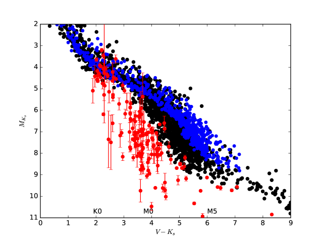
Figure 5: H-R diagram of Pleiades members, nearby stars within 25 pc, and subdwarfs. Pleiades (blue points) are from Rebull et al. (2016) with a uniform parallax of 7.45$\pm$0.3 mas from Gaia DR1 (Gaia Collaboration et al., 2016) assigned to all stars. The $V-K_{s}$ values for the Pleiades members are the dereddened colors from Rebull et al. (2016). Nearby stars (black points) are the same as the gray points in Figure 1 (nearby white dwarfs are beyond the boundaries of this plot). Subdwarfs are shown in red. We omit errorbars for the dwarfs and the Pleiades, but their mean absolute magnitude errors are $\pm$0.05 and $\pm$0.06, respectively. Errors in the horizontal direction are smaller than the points for all three samples.

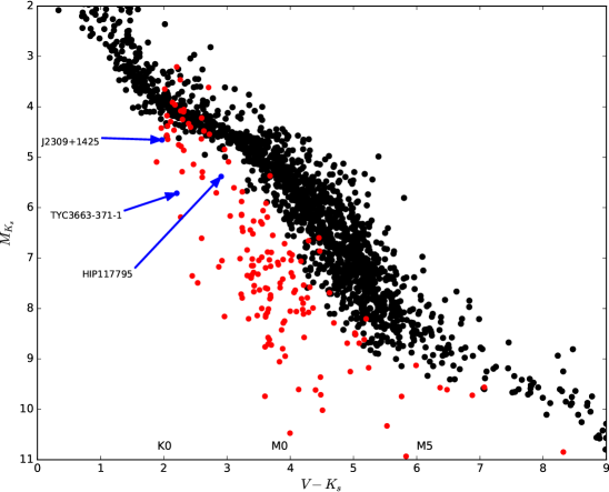
Figure 6: Black points are stars within 25 pc and red points are confirmed subdwarfs. The three labeled blue points are candidate subdwarfs within 60 pc below the main sequence from Gaia DR1 and are discussed in Section 6. The Johnson $V$ magnitudes for these three stars are converted from the Tycho 2 $B$ and $V$ magnitudes. After further analysis, only TYC 3663-371-1 remains a subdwarf candidate.

Spectral types from the literature, including many of our own results, are given in columns 12 and 13 of Table The Solar Neighborhood XLII. Parallax Results from the CTIOPI 0.9-m Program — Identifying New Nearby Subdwarfs Using Tangential Velocities and Locations on the H-R Diagram. Although we do not present any new spectra in this paper, for stars with no spectra available we can make informed estimates of luminosity classes based on the astrometry and photometry data presented here, as discussed in Section 3.1 and 3.2. We assign luminosity class of “VI” to 14 stars we now identify to be subdwarfs, and three as main sequence stars of class “V”. As discussed in Jao et al. (2008), the “sd” prefix often used to classify cool subdwarfs is the same prefix used for hot subdwarfs, even though they are completely different types of stellar objects. The mixed use of “sd” is unique in spectral classification, so we prefer the VI designation. In support of this spectral type moniker, Figures 1,5, 6, and 7 all clearly show a different luminosity class on the Hertzsprung–Russell (H-R) diagram for a given $V-K_{s}$ between (at least) 3 and 6.

4 Notes on Individual Systems

Here we provide additional details of systems worthy of note, listed in order of RA.

0342+1231 (LHS 178) The Yale Parallax Catalog (YPC, van Altena et al. 1995) provides a parallax of 45.1$\pm$12.0 mas for this star and we find 40.19$\pm$2.49 mas, resulting in a weighted mean value of 40.39$\pm$2.44 mas.

0432-3947 (LHS 1678) We detect a possible perturbation with a period of a few years in the astrometric series spanning 12 years, but because it is slight, we have not removed the perturbation to calculate the parallax presented here. Until there is further evidence to support the existence of a currently unseen companion, we consider this is a single star.

0559+0410 (G 99-48AB) Goldberg et al. (2002) found this system to be a double-lined spectroscopic binary, and Soubiran et al. (2010) determined it have [Fe/H]=$-$1.80. Our parallax of 8.06$\pm$1.85 mas is consistent with that provided in Gaia Data Release 1 (hereafter DR1), 7.06$\pm$0.25 mas.

0905-2201 (LHS 2099/2100) This pair of subdwarfs is separated by 6$\farcs$6 at a position angle of 100^∘, corresponding to 326 AU at a distance of 49.4 pc for the weighed mean parallax of 20.24 $\pm$ 0.78 mas. The secondary has $M_{V}$ = 15.69 and $(V-K_{s})$ = 5.53, placing it well below the main sequence in Figure 1 and making it one of the reddest subdwarfs in the sample.

0925+0018 (LHS 2140 and LHS 2139) Gizis & Reid (1997) first reported this common proper motion binary to consist of a subdwarf primary (LHS 2140) and a white dwarf secondary (LHS 2139). LHS 2139 is too faint in our images to measure a reliable parallax, so we adopt the parallax of LHS 2140 for both components. This is one of the very few known subdwarf$+$white dwarf binaries with parallaxes in the solar neighborhood (Monteiro et al., 2006).

0943-1747 (LHS 272) The updated parallax (69.4$\pm$1.02 mas) has a longer time coverage than previously reported in Jao et al. (2011), and supercedes our previous result. This is the fourth nearest known subdwarf system of any spectral type, ranking behind Kapteyn’s Star (GJ 191, M type), $\mu$ Cas AB (GJ 53AB, G and M types), and GJ 451 (K type).

1005-6721 (WT 248) Faherty et al. (2012) reported a parallax of 30.6$\pm$4.6 mas for this object. Our parallax of 41.64$\pm$2.23 places the system within 25 pc, but the weighted mean of 39.54$\pm$2.00 mas is still slightly less than 40 mas.

1110-0247 (G 10-3) Bidelman (1985) classified this star as a K2 dwarf, but it undoubtedly a subdwarf given that Latham et al. (2002) report the star to have $[m/H]=-$2.0. YPC provides a parallax of 28.1$\pm$13.4 mas and we find 7.48$\pm$1.86, yielding a weighted mean value of 7.87$\pm$1.84 mas.

1234+2037 (LHS 334) Our parallax of 17.48$\pm$1.99 mas is consistent with that of Smart et al. (2010), who reported a parallax of 22.1$\pm$3.9 mas. The new weighted mean parallax is 18.43$\pm$1.77 mas.

1358-3938 (SSS 1358-3938) This star has a proper motion of nearly 2$\arcsec$ yr^-1 and we provide the first parallax here, 88.66$\pm$0.80 mas. The star is located on the edge of the main sequence band in the H-R diagram of Figure 1. The photometric distance determined using $VRIJHK$ and the relations of Henry et al. (2004) place this star at 21.2 pc, but our parallax puts it at 11.3 pc. With no previous spectral type available, this large distance mismatch implies this star is likely a subdwarf and we assign it as “VI”. If spectroscopically confirmed, this star would replace LHS 272 as the fourth closest subdwarf system and the third closest M type subdwarf.

1402-2431 (LHS 2852) Gizis (1997) identified this star to be a subdwarf, but it is located on lower edge of the main sequence in the H-R diagram of Figure 1. Haakonsen & Rutledge (2009) found it to have ROSAT X-ray detection of 0.15$\pm$0.03 cnt s^-1. In comparison, the known young star AP Col Riedel et al. (2011) has 0.43$\pm$0.05. In addition, LHS2852 varies by 24 mmag in the $R$ band, the largest variability seen among the 42 subdwarfs studied here. It would be unusual for a subdwarf to be so variable and detected in X-rays, so followup spectroscopy is needed to confirm whether or not the star is a subdwarf. YPC provides a parallax of 39.4$\pm$19.9 mas and we find 57.99$\pm$1.88 mas, yielding a weighted mean value of 57.83$\pm$1.87 mas.

1444-2019 (SSS 1444-2019) This high proper motion (nearly 3.5 $\arcsec$ yr^-1) star was first detected and classified as an M9 subdwarf by Scholz et al. (2004). Recently, Kirkpatrick et al. (2016) re-classified it as a L0 subdwarf. Our parallax of 60.18$\pm$1.62 mas is consistent with the parallaxes reported by Schilbach et al. (2009) (61.67$\pm$2.12 mas) and Faherty et al. (2012) (61.2$\pm$5.1 mas). Together, the three values result in a weighted mean parallax of 60.76$\pm$1.25 mas.

1455-1533 (LHS 385) YPC provides a parallax of 20.4$\pm$5.8 mas and we find 24.43$\pm$1.51 mas, resulting in a weighted mean value of 24.17$\pm$1.46 mas.

1506+1321 (2MA1506+1321) Gizis et al. (2000) reported this object to be an L3 dwarf, implying that it is a brown dwarf because it is later than the L2 type found by Dieterich et al. (2014) at the stellar/substellar boundary. It is too faint for $V$ band photometry at the 0.9-m, so no DCR correction was made for this field; however, because this field was observed in the $I$ band, any DCR correction is minimal. Gagné et al. (2014) flagged this object with a 100% probability to be a young field object. The object shows three signs of youth: (1) a triangular-shaped H-band continuum, (2) redder-than-normal colors for its assigned spectral type, and (3) signs of low gravity from atmospheric model fitting. With a relatively slow tangential velocity of 58.3 km s^-1, it does not have the typical high velocity of an old subdwarf, so it is likely a young brown dwarf for which we provide the first parallax of 87.08$\pm$1.58 mas.

1539-5509 (LHS 401) YPC provides a parallax of 38.4$\pm$9.6 mas and we find 38.67$\pm$1.68 mas, resulting in a weighted mean value of 38.66$\pm$1.65 mas.

1610-0040 (LSR1610-0040 AB) is an important subdwarf system, given that it promises to yield accurate masses for a pair of very cool subdwarfs. This system was first detected and classified as an early type L subdwarf by Lépine et al. (2003). Cushing & Vacca (2006) later showed the system to have a peculiar spectrum with an ambiguous assignment of dwarf or subdwarf type. Dahn et al. (2008) reported the first trigonometric parallax of 31.02$\pm$0.26 mas, detected a clear photocentric orbit with a semi-major axis of 8.91 mas, and classified it as type “sd?M6pec”. Recently, Koren et al. (2016) estimated the masses of the primary and unseen secondary using updated astrometry from Dahn et al. (2008) and radial velocity data from Blake et al. (2010) and found masses of 0.09–0.10 $M_{\odot}$ and 0.06 – 0.075 $M_{\odot}$. Our dataset of 9.98 years also detects a large astrometric perturbation (see Figure 2) with a period of 634.8 days, nearly identical to the period of 633 days found by Koren et al. (2016), even though their timespan is 10.2 years. We measure a photocentric semi-major axis of 8.25$\pm$0.63 mas, but Koren et al. (2016) has 9.89$\pm$0.25 mas. Although both USNO and CTIO parallax programs use “I” filters, their bandpasses are different. The effective central wavelength and filter band width for USNO and CTIO are 8074Å/1890Åand 8118Å/1415Å, respectively. These two different bandpasses may cause the slight difference in the photocentric semi-major axis.

Schilbach et al. (2009) reported a parallax of 33.1$\pm$1.32 mas, and an updated USNO parallax of 30.73$\pm$0.34 mas, calculated using an Markov chain Monte Carlo simulation, is given in Koren et al. (2016). After removing the perturbation of the photocenter shown in Figure 2, we find a parallax of 32.26$\pm$0.48 mas. The final weighted mean parallax from these three measurements is 31.32$\pm$0.27 mas.

1718-4326 (LHS 440 AB) Jao et al. (2008) reported this to be a M1.0 subdwarf and Jao et al. (2011) first reported the possible unseen companion based upon a photocentric perturbation. We have extended the coverage from 9 years in Jao et al. (2011) to $\sim$15 years in this work, yielding the perturbation curve shown in Figure 2. Because of the very long orbital period for the system, we do not detect a full photocentric orbit yet. The parallax of 39.56$\pm$1.02 mas presented in Table 1 has had the perturbation removed and supersedes previously reported values in Jao et al. (2005) and Jao et al. (2011).

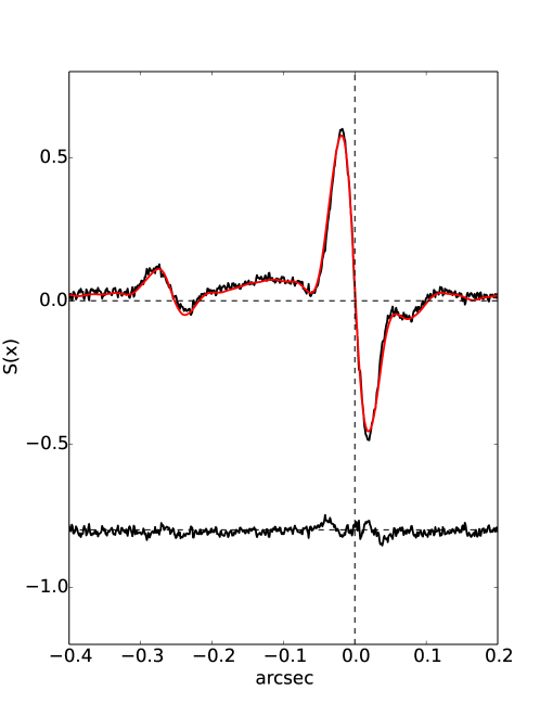
Figure 4: The “S-curve” along the X-axis from a Hubble Space Telescope Fine Guidance Sensor observation of LHS 440 AB. The black line on the top represents the data and the red line is the best fit. The residuals to the fit are shown on the bottom of the plot. The secondary is clearly seen at a separation of 256 mas with a $\Delta_{F583W}=$2.03. Note that the X-axis is not the direction of RA because of the HST’s roll angle at the observation epoch. The binary is not resolved along the Y-axis, so is not shown here.

We used the FGS1r (Fine Guidance Sensors) on the Hubble Space Telescope to resolve this system in Cycle 16 on April 10th, 2009, with scan duration of 1301 sec and scan lengths of 6″. Observations were made through the F583W filter, which provides magnitude differences similar to the $V$ band in the Johnson system. The standard strfits routine in the IRAF/STSDAS package was used to measure the separation, position angle, and magnitude difference between the two components. Additional details of the reduction procedure can be found in the HST/FGS Data Handbook http://www.stsci.edu/hst/fgs/documents/datahandbook/. The calibrator is LHS 73, which is also a subdwarf and was observed in the same HST observing Cycle. LHS 440 AB was successfully resolved along the X-axis, as shown in Figure 4. The pair was not resolved along the Y-axis at this epoch, indicating a separation of $\pm$ 10 mas, so we cannot calculate the companion’s separation and position angle. The magnitude difference is 2.03 mag in the F583W filter. Henry et al. (1999) presented a conversion from $\Delta m_{F583W}$ to $\Delta V$ using $B-V$ colors, but no $B$ photometry is available for the components, and the relations used in the absence of $B$ photometry apply to dwarfs rather than subdwarfs. Assuming for now that $\Delta V$ $\approx$ 2, we find $M_{V}$ = 11.13 and 13.13 for the components. From the mass-luminosity relation for main sequence red dwarfs of Benedict et al. (2016), this implies masses of 0.33 and 0.19 $M_{\odot}$, but again because these are subdwarfs rather than dwarfs, we emphasize that these should be considered only crude estimates.

1750-5636 (LHS 456) YPC provides a parallax of 39.2$\pm$12.6 mas and we find 39.87$\pm$1.43, resulting in a weighted mean value of 39.86$\pm$1.42 mas.

1809-6154 (SCR1809-6154 AB) The separation of these two stars is 19$\farcs$2 at a position angle of 270.6^∘. Because the primary star is very close to a background star, no variability is reported for the primary and only frames with seeing less than 1$\farcs$4 were kept for the astrometric reduction. The weighted mean parallax for the two components is 5.50$\pm$1.16 mas.

1809+2755 (G 182-41AB) This is a double-lined spectroscopic binary with [Fe/H]=$-$1.0 (Goldberg et al., 2002), clearly indicating that it is a subdwarf. Our parallax of 9.96$\pm$2.33 mas places the pair at $\sim$100 pc, indicating that the resolution needed to determine masses will prove difficult.

2101+0307 (USN 2101+0307AB) The combined photometry make this system elevated on the H-R diagram. We do not have a spectrum for this system. Becasue of its location on the H-R diagram, we temporarily assign its luminosity class as “V”.

2239-3615 (LHS 3841AB) Friedrich et al. (2000) showed this star to have a combined spectrum of helium-rich white dwarf and an M dwarf using a spectrograph with a coverage of 3800Å to 9200Å. Reid & Gizis (2005) later identified the red dwarf to be an M2.5 subdwarf with a wavelength coverage of 6200Å to 7500Å and estimated the distance to be 19 pc. However, we determine a parallax of 12.13$\pm$1.47 mas, placing the system at $\sim$80 pc. The erroneous distance estimate was likely due to excess flux from the white dwarf not being considered. Farihi et al. (2010) used the Advanced Camera for Surveys High-Resolution Camera on the Hubble Space Telescope in an attempt to resolve this system using the F814W filter, but LHS3841 AB was not resolved. Over 4.2 years of astrometric observations, we do not detect any perturbation of the photocenter position.

2343-2409 (LHS 72 and LHS 73) Both components are subdwarfs (Rodgers & Eggen, 1974; Reylé et al., 2006; Jao et al., 2008), separated by 1$\farcm$6 at position angle of 153^∘. The primary, LHS 72, has a parallax of 37.6$\pm$8.9 mas in the YPC, but no separate parallax is given for LHS 73. We find parallaxes of 35.20$\pm$1.63 mas and 32.73$\pm$1.44 mas for the primary and secondary, respectively, which agree within 2$\sigma$. The weighted mean of all three parallax measurements is 33.87$\pm$1.07 mas.

5 Discussion: Observational Differences between Dwarfs and Subdwarfs

Subdwarfs are low-metallicity stars that have historically been discovered through proper motion surveys, spectroscopic surveys, or color index searches. Historically, the extensive proper motion surveys by Luyten and Giclas have been the primary sources for finding subdwarfs (Ryan & Norris, 1991; Bessell, 1982; Gizis, 1997). Recent new proper motion surveys with fainter magnitude limits like SuperBLINK (Lépine & Shara, 2005), SuperCOSMOS-RECONS (Subasavage et al., 2005), and SIPS (Deacon et al., 2005) have discovered many new metal-deficient high proper motion subdwarf candidates. To confirm that these candidates are, indeed, cool subdwarfs, spectroscopic observations are typically necessary, such as those by (Scholz et al., 2004; Lépine et al., 2007; Jao et al., 2008; Zhang et al., 2013). Large sky spectroscopic surveys like SDSS and LAMOST have also provided systematic ways to identify cool subdwarfs (West et al., 2004; Zhong et al., 2015). Finally, because subdwarfs have different colors from dwarfs, infrared colors from the all sky infrared surveys 2MASS and WISE have been used to identify local stellar and sub-stellar subdwarfs (Burgasser et al., 2007; Kirkpatrick et al., 2011).

Here we discuss two other observational methods that allow the identification of cool subdwarf candidates among stars in the solar neighborhood. These methods utilize the astrometry and photometry data presented in this paper to evaluate tangential velocities (using astrometry only), and positions on the H-R diagram (using both astrometry and photometry) to reveal cool subdwarfs. After outlining how subdwarfs can be identified, we apply these two methods on samples from Gaia DR1 and the MEarth Project to identify new nearby subdwarfs.

5.1 Tangential Velocity

Kinematic methods that map the motions of stars in our Galaxy have been used to identify subdwarfs because over billions of years, old low-metallicity subdwarfs are generally disk-heated to higher spatial velocities. The challenge in using $UVW$ kinematics to separate subdwarfs from dwarfs is that both trigonometric parallaxes and radial velocities are required for each candidate star. Nonetheless, several efforts have revealed trends. Ryan & Norris (1991) found that while $\sigma_{U}$, $\sigma_{V}$ and $<$V$>$ are independent of metallicity, the vertical velocity dispersion, $\sigma_{W}$, increases with decreasing metallicity. They use $\sigma_{W}$ values to separate over 770 FGKM stars from the NLTT catalog, among which they flagged 115 K and 4 M subdwarfs. A study by Arifyanto et al. (2005), based on 742 nearby metal-poor stars from Carney et al. (1994), reported that halo stars with [Fe/H]$<$$-$1.6 have a low mean rotational velocity around the Galaxy and a radially elongated velocity ellipsoid, while stars with $-$1.6$<$[Fe/H]$<$$-$1 have disk-like kinematics. Based on a limited sample of 69 subdwarfs with both parallaxes and radial velocities, Gizis (1997) found different mean Galactic rotation velocities between different sub-types of subdwarfs, and noted that overall, subdwarfs move faster than regular M dwarfs. A recent result by Savcheva et al. (2014), using a much larger sample (3517) drawn from SDSS data, showed the same trend as Gizis (1997).

Without radial velocities, many authors have turned to using a tangential velocity cutoff to select subdwarfs in lieu of complete $UVW$ motions. As a benchmark, Hawley et al. (1996) reported that a northern sample of 514 M dwarfs has an average tangential velocity of 43.8 km s^-1. In order to get an uncontaminated sample of halo stars from the Giclas high proper motion survey, Schmidt (1975) imposed a hard limit on tangential velocity of 250 km s^-1 to determine the luminosity function of halo stars. Later, Gizis & Reid (1999) used various tangential velocity cutoffs to select halo stars from the reduced proper motion diagram in order to revise the luminosity function of the halo population. Stars having $V_{tan}>$ 75 km s^-1 were flagged as being M extreme subdwarf candidates, while stars with $V_{tan}>$ 125 km s^-1 were flagged as being the M regular subdwarf candidates. Digby et al. (2003) used a tangential velocity of 200 km s^-1 to select their subdwarf candidates based on the reduced proper motion diagram.

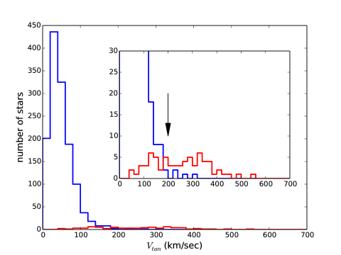
Figure 3: A histogram of tangential velocities for stars in different stellar populations. K and M type stars within 25 pc are represented with the blue line, with peak near 30 km s^-1. Tangential velocities of 167 subdwarfs from our work and the literature are shown in red. The inset panel shows a zoomed plot. The arrow marks the 200 km s^-1 limit we use to select K and M subdwarfs that are found at larger tangential velocities. The four stars with $V_{tan}>$ 200 m s^-1 shown in blue are known subdwarfs within 25 pc.

Now that we have parallaxes for a relatively large sample of K and M subdwarfs, we use the sample to determine an appropriate $V_{tan}$ cutoff that can be used to identify subdwarfs. Figure 3 illustrates $V_{tan}$ distributions of main sequence dwarfs and subdwarfs. The 1324 nearby K and M dwarfs with parallaxes placing them within 25 pc were selected using spectral types and a color cutoff of $V-K_{s}$$>$ 1.9, and are represented with the blue curve. The red line indicates the 167 K and M subdwarfs observed during our CTIOPI program with new or revised parallaxes from RECONS, supplemented with confirmed subdwarfs collected from the literature (Ryan & Norris, 1991; Carney et al., 1994; Hawley et al., 1996; Gizis, 1997; Cayrel de Strobel et al., 2001; Burgasser et al., 2003; Lépine et al., 2003; Woolf & Wallerstein, 2005; Jao et al., 2009; Wright et al., 2014). This plot shows that most K and M dwarfs in the solar neighborhood have $V_{tan}$ $<$ 100 km s^-1 with a peak in the distribution at 30 km s^-1, consistent with the average tangential velocity discussed in Hawley et al. (1996) near 45 km s^-1. Adopting a cutoff of $V_{tan}$ = 200 km s^-1 reveals only four stars at higher $V_{tan}$ values, each of which is, in fact, a known nearby subdwarf. Thus, there are no known main sequence K and M dwarfs within 25 pc with $V_{tan}$ $>$ 200 km s^-1. Unfortunately, this cutoff permits us to identify only 57% (95/167) of (fast-moving) subdwarfs and excludes the remaining 43% with slower $V_{tan}$ values. Nonetheless, although solar neighborhood stars with tangential velocities less than 200 km s^-1 comprise a mixed population of young, middle-aged, and old stars, virtually all nearby stars with tangential velocities greater than 200 km s^-1 are confirmed subdwarfs. This cutoff may be used with confidence to select samples of cool subdwarfs.

5.2 Hertzsprung-Russell diagram

In Figure 1, we use $M_{V}$ and $(V-K_{S})$ to illustrate the locations of the sample of objects targeted here. We show an additional H-R diagram in Figure 5 using $V-K_{s}$ vs. $M_{K}$, rather than $M_{V}$. Stars within 25 pc on the main sequence are shown in black, overlaid with members of the Pleiades (Rebull et al., 2016) in blue and the 167 subdwarfs discussed in the previous section in red. These three sets of stars of various ages and metallicities are merged blueward of $V-K_{s}\approx$ 2 and brighter than $M_{K}\approx$ 4. In contrast, the three samples form clear “bands” in this diagram in the redder, fainter portion of the diagram. Based on Figure 5, we conclude that: (1) the general trend shows that the populations’ ages, from $\sim$100 Myr for the Pleiades, to mixed ages of a few Gyr for disk stars, to 6-9 Gyr for subdwarfs), as well as differing metallicities, causes the shift in the stellar distribution on the H-R diagram. (2) Early K-type young stars, dwarfs, and subdwarfs are indistinguishable in the H-R diagram of Figure 5. (3) There is no prominent void in the distribution of subdwarfs from (at least) $V-K_{S}$ = 2–7 in the observational H-R diagram. Gizis (1997) identified many cool subdwarfs spectroscopically and established an important foundation in subdwarf studies. He found a void on his H-R diagram that lacked “sdM” subdwarfs with 2.2$<V-I<$2.8, corresponding to 3.9$<V-K_{s}<$5.2. Although the number of stars in this region is still smaller than at bluer colors, the void has begun to fill in because new subdwarf identification efforts since have increased the number of subdwarfs in this color range. Given that the metallicity distribution is smooth instead of clumped (Gizis, 1997), we expect more subdwarfs in this color range should be unveiled in the future.

6 Subdwarfs Identified using $V_{tan}$ and the H-R diagram

We applied these two methods for identifying new subdwarfs using the latest large sets of parallaxes recently released in Gaia DR1 (Gaia Collaboration et al., 2016, GAIADR1) which contains stars in common between the Tycho-2 Catalogue and Gaia mission, and by the MEarth Project which focuses on nearby M dwarfs (Dittmann et al., 2014).

6.1 the Gaia DR1 Catalog

We extracted 9494 targets within 60 pc from Gaia DR1. Not all stars have Johnson V magnitudes, so a conversion ($V=V_{T}-0.09*(B_{T}-V_{T})$) from the Tycho 2 catalog was used to convert Tycho 2 $V$ magnitudes to the standard Johnson $V$ filter. None of these 9494 targets has a tangential velocity greater than 200 km s^-1. We identified only three stars clearly below the main sequence on the HR diagram. These three candidates are plotted in Figure 6 and discussed below. We find that two stars are subdwarf candidates and the third is not a subdwarf. The paucity of intrinsically faint new subdwarf candidates is not surprising given that only stars bright enough to be observed by Tycho have parallaxes in Gaia DR1.

(0051+5629) TYC 3663-371-1 This star is almost two magnitudes fainter than stars in the center of the main-sequence band in Figure 6, providing strong evidence that it is a K subdwarf. No metallicity measurement is found in the literature.

The star is listed as a companion to a G star (HD 4868) in SIMBAD, and The Washington Double Star Catalog lists the two stars as a visual binary (WDS 00515+5630AB) with a separation of 40$\farcs$6 (Høg et al., 2000). Gaia DR1 reports a parallax of 21.84$\pm$0.81 for TYC 3663-371-1, but no parallax for HD 4868. HD 4868 does have a parallax of 16.28$\pm$0.79 in the Hipparcos catalog (van Leeuwen, 2007), which is $\sim$5$\sigma$ offset from TYC 3663-371-1’s value. Both stars have similar proper motions in Tycho 2, but the proper motion for TYC 3663-371-1 in Gaia DR1 (see Table 3) is very different. Because of the parallax and proper motion differences, we do not believe these two stars form a physically bound system.

(2309+1425) LSPM J2309+1425 = TYC 1167-683-1 There is an X-ray source in the direction of this star, which is found in a region of high Galactic latitude molecular clouds (Li et al., 2000). The ROSAT catalog shows an X-ray source with $f_{x}/f_{opt}=$$-$1.93 for this star and Li et al. (2000) reported detection of H$\alpha$ emission. Cutispoto et al. (2002) even set an upper limit on the lithium equivalent width of 0.8 milli-Angstrom. The lithium line, X-ray and H$\alpha$ emission typically indicate youth, so this star is not a subdwarf. In addition, as shown in Figure 6, stars of different ages merge at this color on the H-R diagram, and this star is barely offset from main sequence stars.

The star is listed as a companion to HIP 114378 in SIMBAD, and The Washington Double Star Catalog lists the two stars as a visual binary (WDS 23100+1426AB) with a separation of 31$\farcs$7 (Høg et al., 2000). Both stars have parallaxes and proper motions in Gaia DR1, given in Table 3. As with TYC 3663-371-1, the distances and proper motions given in Table 3 do not support that the two components are physically bound. Their parallaxes differ by $\sim$4$\sigma$ and the proper motions in Gaia DR1 do not match. Hence, these two stars are likely not associated.

(2353+5956) HIP 117795 This star has no metallicity measurement in the literature. Sperauskas et al. (2016) reported a radial velocity of $-$285.9$\pm$0.2 km s^-1. Although this star’s tangential velocity (11.2 km s^-1) is less than 200 km s^-1, the Gaia parallax (37.49$\pm$0.23 mas) and proper motion, combined with the radial velocity measurement, yield $U,V,W$ = (-114, -262, $+$12). Thus, kinematically, HIP 117795 is very different from nearby disk M dwarfs (Hawley et al., 1996) and it is about one magnitude below the center of the main sequence in Figure 6. As we discussed earlier, Arifyanto et al. (2005) showed halo stars with [Fe/H]$<$$-$1.6 have low mean galactic rotational velocity, but their velocities range from $+$200 to $-$200 km s^-1. As for stars with [Fe/H]$>$$-$1.0 in Arifyanto et al. (2005), their galactic rotational velocities are clustered around $+$200 km s^-1. The direction and velocity of HIP 117795’s $V$ indicates it has a retrograde motion and is much faster than the limit shown in Arifyanto et al. (2005) for halo stars. By combining its kinematic and location on the H-R diagram, we think it is likely a nearby K subdwarf.

6.2 The MEarth Project

The MEarth Project released 1507 parallaxes of nearby M dwarfs (Dittmann et al., 2014), but after taking into account companions, there are a total of 1511 entries. Although this list of stars lacks spectral classifications, most of them should be M dwarfs, as MEarth is targeting M dwarfs. After calculating each star’s tangential velocity, we find that only LSPM J2107+5943 (LHS 64) has $V_{tan}>200$ km s^-1, and it is a known nearby cool subdwarf (Gizis, 1997).

To reveal additional subdwarfs, we also wish to check the locations of these stars on the H-R diagram. (Dittmann et al., 2014) provide only 2MASS $J$ and $K_{s}$ magnitudes, and unlike the $V-K_{s}$ color shown in Figure 5, $J-K_{s}$ does not clearly differentiate young M dwarfs, disk M dwarfs, and M subwarfs on the H-R diagram. In addition, not all 1511 stars have Johnson $V$ magnitudes, so it is not possible to overplot the entire sample on the same scale as shown in Figure 5 for comparison.

In order to create a set of uniform photometry, we cross-matched the stars with entries in the recent PanSTARRS data release (Flewelling et al., 2016) and extracted $g$ and $r$ magnitudes. In the PanSTARRS data release, high proper motion stars usually, but not always, have multiple entries and coordinates because of the different epochs of PanSTARRS images, resulting in several lines of matches for a given coordinate and search radius. Presumably, all of these entries are the same star moving across the sky. On the other hand, if a star has only one correct entry in PanSTARRS, we may also get multiple lines because of several sources within the search radius. In order to separate correct matches from false ones, we apply multiple steps to extract PanSTARRS photometry. First, we submitted MEarth stars’ equinox and epoch J2000 coordinates to the PanSTARRS site (http://archive.stsci.edu/panstarrs/search.php) and set the search radius to 0$\farcm$5. We calculated the mean epoch from all entries found in this search. We then slid the MEarth stars’ coordinates from J2000 to that mean epoch using the MEarth proper motions. The second search was done by querying these new coordinates but with a reduced search radius of 0$\farcm$1, and “PSFMag” values were extracted. Most stars have only one match in the PanSTARRS catalog at this mean epoch with the smaller search radius, but for those stars with multiple matches, a mean photometric magnitude at a given filter was calculated, with its standard deviation required to be less than 0.5 mag to eliminate mixing background sources — individual photometric measurements for a given filter typically have errors less than 0.04 mag. In total, 1349 stars had both $g$ and $r$ magnitudes that were then converted to Johnson $V$ magnitudes using the equation $V=g-0.5784*(g-r)-0.0038$, which is available at SDSS’s website (http://www.sdss3.org/dr8/algorithms/sdssUBVRITransform.php#West2005). We note that PanSTARRS filter bandpasses differ slightly from those of the SDSS filters.

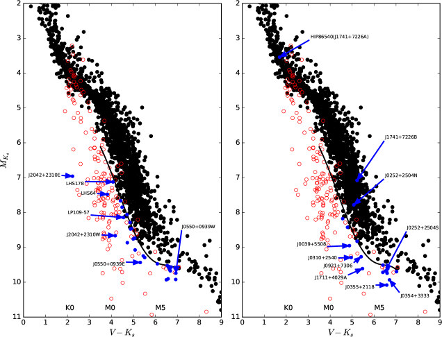
Figure 7: Black points are stars within 25 pc and red open circles are confirmed subdwarfs; points are the same in both panels. Blue stars in both panels are subdwarf candidates. The black curve is the same in both panels and divides main sequence stars from subdwarfs. The curve is defined by $M_{K_{s}}=0.019\times color^{5}-0.42\times color^{4}+3.56\times color^{3}-14.11\times color^{2}+27.29\times color-15.99$, where “$color$” is $V-K_{s}$. The left panel highlights stars below the curve that are subdwarf candidates. The right panel highlights stars (generally) below the curve that have been spectroscopically classified as main sequence M dwarfs. Labeled stars are discussed in section 6.

Rather than relying on our converted $V$ magnitudes, we choose to identify possible subdwarfs empirically by using cutoffs in $M_{Ks}$ instead of $M_{V}$ because the 2MASS $K_{s}$ photometry is uniformly consistent. The fifth-order polynomal line shown in Figure 7 was established based on where known subdwarfs (represented with red points) are found relative to main sequence stars (black points). The 51 MEarth stars located on or below this dividing line are considered to be subdwarf candidates and are listed in Table The Solar Neighborhood XLII. Parallax Results from the CTIOPI 0.9-m Program — Identifying New Nearby Subdwarfs Using Tangential Velocities and Locations on the H-R Diagram. Three highlighted stars above the lines in the two panels of Figure 7 are discussed below.

Among these 51 stars are 30 subdwarf candidates shown with blue points in the left panel of Figure 7. Blue points in the right panel represent 20 stars that have been spectroscopically identified as regular dwarfs in the literature and one (LSPM J1012+2113) that is a close double with a suspect position in Figure 7..

6.2.1 New Subwarf Candidates

Among the 30 subdwarf candidates selected using this method, LHS 64, LHS 178 and LP 109-57 are previously identified M subdwarfs and are labeled in the left panel of Figure 7. Thus, we present here 27 new subdwarf candidates, listed in Table The Solar Neighborhood XLII. Parallax Results from the CTIOPI 0.9-m Program — Identifying New Nearby Subdwarfs Using Tangential Velocities and Locations on the H-R Diagram. We identify two wide subdwarf binary systems, LSPM J0550+0939EW and LSPM J2042+2310EW, each with both components falling below the dividing line and labeled in Figure 7. In particular, LSPM J2042+2310E is $\sim$3 full magnitudes below the main sequence.

6.2.2 Spectroscopically Confirmed M Dwarfs

Twenty stars in 17 systems shown in the right panel of Figure 7 were previously identified as M dwarfs in the literature. Several of these stars are worth discussing to outline why this group of stars should not be considered subdwarfs.

LSPM J1741+7226B is an M4 dwarf (Alonso-Floriano et al., 2015) located in the center of main-sequence in Figure 7. It is a wide common proper motion companion to a bright star, HIP 86540/G 258-16A (Lépine & Bongiorno, 2007). The MEarth parallax is 77.6$\pm$5.0 mas for LSPM J1741+7226B, so initially this star was identified as a subdwarf candidate using the H-R diagram. However, Gaia DR1 reports a parallax of 33.17$\pm$0.21 mas for the primary, so the weighted mean parallax moves LSPM J1741+7226B upward to the current location shown in Figure 7. This revised location on the H-R diagram matches its luminosity, as classified by Alonso-Floriano et al. (2015).

Six stars — LSPM J0039+5508 (LHS 6009), LSPM J0310+2540, LSPM J0354+3333, LSPM J0355+2118, LSPM J0921+7306 (LHS2126), and LSPM J1711+4029A (G203-50A) — highlighted in the right panel of Figure 7, are well below the main sequence, implying that they are subdwarfs, but their locations contradict their reported spectral types. Their 2MASS $K_{s}$ magnitudes should be reliable, so either their converted $V$ magnitudes or MEarth parallaxes are in error. For example, LSPM J0039+5508 has Johnson $V=$14.17 from Weis (1988), resulting in $V_{J}-K_{s}=$4.93 compared to $V_{converted}-K_{s}=$4.88. The 0.05 magnitude difference is not sufficient to relocate this star horizontally onto the main sequence, so if the star is indeed on the main sequence, the parallax is incorrect. Thus, we suspect that the parallaxes for these six stars also need to be revised, as is the case for LSPM J1741+7226.

LSPM J0252+2504N (G36-39) and J0252+2504S form a wide common proper motion pair. The primary star is clearly on the main sequence and has a spectral type of M4.5 (Reid et al., 2004). Even though the secondary is below our empirical dividing line, it should be considered a dwarf. Thus, several of the stars very near the cutoff line are likely just misplaced in the diagram because of slightly incorrect $V$ estimates or parallaxes.

7 The Future of Finding Nearby Subdwarfs

In the past 20 years, thousands of subdwarfs have been identified through all-sky spectroscopic surveys or targeted individual spectroscopic observations. However, without trigonometric parallaxes, we cannot pinpoint their locations on the H-R diagram and link them to their originally defined character: “dwarfs below the main sequence” (Kuiper, 1939). Since Bessel measured the first parallax in 1838 for 61 Cygni, trigonometric parallaxes continue to be one of the most essential measurements in stellar astrophysics. In this paper we contribute parallaxes for 51 systems, including 37 systems for which these are the first parallaxes, of which 15 have proper motions of at least 1$\arcsec$ yr^-1. We find that most of the stars targeted here turn out to be cool subdwarfs.

We describe two reliable methods for revealing subdwarfs in the solar neighborhood. By using astrometry alone, we find that if a nearby K or M dwarf has a tangential velocity greater than 200 km s^-1 it is almost certainly a subdwarf. Using accurate trigonometric parallaxes and $V$ and $K_{s}$ photometry such as that presented here, we show that by carefully placing stars on the H-R diagram we can also identify cool subdwarfs. In the next a few years, the Gaia and LSST efforts will measure countless high precision parallaxes, proper motions, and photometric values for stars throughout the sky. We plan to apply these two methods to identify a large number of nearby low metallicity subdwarfs, so that we can unveil more of the missing Galactic relics in the solar neighborhood.

8 Acknowledgments

The astrometric observations reported here began as part of the NOAO Surveys Program in 1999 and continued on the CTIO 0.9-m via the SMARTS Consortium starting in 2003. We gratefully acknowledge support from the National Science Foundation (grants AST 05-07711, AST 09-08402, and AST 14-12026), NASA’s Space Interferometry Mission, and Georgia State University, which together have made this long-term effort possible. We also thank the members of the SMARTS Consortium, who enable the operations of the small telescopes at CTIO, as well as the supporting observers at CTIO, specifically Edgardo Cosgrove, Arturo Gómez, Alberto Miranda, and Joselino Vásquez.

The HST-FGS observations were supported under program 11943 by NASA through grants from the Space Telescope Science Institute, which is operated by the Association of Universities for Research in Astronomy, Inc., under NASA contract NAS5-26555.

This research has made use of the SIMBAD database, operated at CDS, Strasbourg, France. This publication makes use of data products from the Two Micron All Sky Survey, which is a joint project of the University of Massachusetts and the Infrared Processing and Analysis Center/California Institute of Technology, funded by the National Aeronautics and Space Administration and the National Science Foundation. This work also has made use of data from the European Space Agency (ESA) mission Gaia (https://www.cosmos.esa.int/gaia), processed by the Gaia Data Processing and Analysis Consortium (DPAC, https://www.cosmos.esa.int/web/gaia/dpac/consortium). Funding for the DPAC has been provided by national institutions, in particular the institutions participating in the Gaia Multilateral Agreement.

The Pan-STARRS1 Surveys (PS1) and the PS1 public science archive, which were used for this study, have been made possible through contributions by the Institute for Astronomy, the University of Hawaii, the Pan-STARRS Project Office, the Max-Planck Society and its participating institutes, the Max Planck Institute for Astronomy, Heidelberg, the Max Planck Institute for Extraterrestrial Physics, Garching, The Johns Hopkins University, Durham University, the University of Edinburgh, the Queen’s University Belfast, the Harvard-Smithsonian Center for Astrophysics, the Las Cumbres Observatory Global Telescope Network Incorporated, the National Central University of Taiwan, the Space Telescope Science Institute, the National Aeronautics and Space Administration under Grant No. NNX08AR22G issued through the Planetary Science Division of the NASA Science Mission Directorate, the National Science Foundation through Grant No. AST-1238877, the University of Maryland, Eotvos Lorand University (ELTE), the Los Alamos National Laboratory, and the Gordon and Betty Moore Foundation.

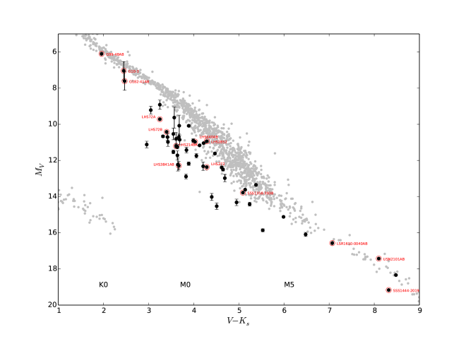
Figure 1: An observational H-R diagram, using $M_{V}$ vs. $V-K_{s}$, is shown for 53 stars (dark filled circles) in the 51 systems outlined in Tables 1 and The Solar Neighborhood XLII. Parallax Results from the CTIOPI 0.9-m Program — Identifying New Nearby Subdwarfs Using Tangential Velocities and Locations on the H-R Diagram. Two objects, the brown dwarf 2MA 1506$+$1321 and the white dwarf LHS 2139, do not have both $V$ and $K_{s}$ magnitudes and are not shown. For comparison, gray points represent stars within 25 pc, with data taken primarily from the Yale Parallax Catalog, Hipparcos results, our RECONS astrometry/photometry program, the MEarth Project, and Gaia DR1. It is clear that most of the stars presented in this work are below the main sequence and are subdwarfs. Red circles highlight interesting systems discussed in Section 4. Errorbars in the horizontal direction are smaller than the points.

Figure 2: Nightly mean astrometric residuals in right ascension and declination are shown for LSR 1610-0040 AB and LHS 440 AB. The astrometric signatures of each system’s proper motion and parallax have been removed. Solid-line curves show the best fits to the perturbations and these fits have been removed when determining the proper motions and trigonometric parallaxes presented here. [To Editor: Please arrange two plots horizontally.]

Table 1: Astrometry Results

Name	RA	DEC	Filt	Nsea	Nfrm	Coverage	Years	Nref	$\pi$(rel)	$\pi$(corr)	$\pi$(abs)	$\mu$	P.A.	$V_{tan}$	Note
	(J2000.0)								(mas)	(mas)	(mas)	(mas/yr)	(deg)	(km/s)
(1)	(2)		(3)	(4)	(5)	(6)	(7)	(8)	(9)	(10)	(11)	(12)	(13)	(14)
First Trigonometric Parallaxes
LHS 1048	00 15 33.51	$-$35 11 47.6	I	8s	69	2005.71–2012.89	7.18	8	24.47$\pm$1.06	1.64$\pm$0.16	26.11$\pm$1.07	949.4$\pm$0.4	100.1$\pm$0.04	172.4
LHS 127	00 55 43.89	$-$21 13 07.1	I	8s	61	2003.94–2012.94	8.99	7	14.98$\pm$1.10	0.52$\pm$0.03	15.50$\pm$1.10	1227.7$\pm$0.4	99.2$\pm$0.03	375.6
LEHPM 1-1628	01 31 05.40	$-$50 25 10.0	I	7s	50	2005.72–2012.94	7.22	9	10.05$\pm$1.83	0.50$\pm$0.06	10.55$\pm$1.83	1083.0$\pm$0.6	142.1$\pm$0.06	486.5
LHS 1257	01 31 30.82	$+$10 01 29.7	I	7s	48	2005.80–2012.81	7.01	7	20.00$\pm$2.25	0.96$\pm$0.13	20.96$\pm$2.25	929.6$\pm$0.7	158.1$\pm$0.08	210.2
LHS 150	02 07 23.26	$-$66 34 11.6	V	9s	69	2003.95–2012.70	8.75	8	84.91$\pm$1.83	1.24$\pm$0.12	86.15$\pm$1.83	1774.2$\pm$0.7	78.2$\pm$0.04	97.6
LHS 1490	03 02 06.36	$-$39 50 51.9	I	8s	87	2007.55–2015.96	8.41	9	70.46$\pm$1.62	0.31$\pm$0.02	70.77$\pm$1.62	850.6$\pm$0.8	220.6$\pm$0.11	57.0
LHS 1678	04 32 42.63	$-$39 47 12.3	V	11s	111	2003.95–2016.05	12.09	8	49.90$\pm$1.14	1.67$\pm$0.14	51.57$\pm$1.15	1001.0$\pm$0.3	166.8$\pm$0.03	92.0	!
LEHPM 1-3861	05 00 15.78	$-$54 06 27.5	I	6s	42	2005.90–2011.00	5.08	10	15.58$\pm$1.54	0.63$\pm$0.04	16.21$\pm$1.54	1057.7$\pm$1.1	169.2$\pm$0.10	309.3
LSR 0609+2319	06 09 52.43	$+$23 19 12.8	I	6c	58	2006.05–2011.00	4.95	11	20.88$\pm$1.39	1.68$\pm$0.21	22.56$\pm$1.41	1109.5$\pm$0.8	131.3$\pm$0.08	233.1
SCR 0701-0655	07 01 17.79	$-$06 55 49.4	I	4s	49	2009.08–2011.20	3.12	9	4.68$\pm$0.98	1.58$\pm$0.14	6.26$\pm$0.99	583.3$\pm$0.8	185.0$\pm$0.12	441.6
SCR 0708-4709	07 08 32.04	$-$47 09 30.6	V	5s	54	2007.19–2011.23	4.04	9	11.24$\pm$1.34	0.81$\pm$0.10	12.05$\pm$1.34	402.2$\pm$1.0	114.8$\pm$0.28	158.3
SCR 0709-4648	07 09 37.28	$-$46 48 58.8	R	4c	53	2008.14–2011.23	3.09	9	13.20$\pm$1.41	1.22$\pm$0.16	14.42$\pm$1.42	391.5$\pm$1.2	9.0$\pm$0.30	128.7
SCR 0816-7727	08 16 35.65	$-$77 27 11.7	V	3s	36	2010.01–2012.19	2.17	9	12.72$\pm$1.69	0.94$\pm$0.09	13.66$\pm$1.69	688.3$\pm$2.2	324.8$\pm$0.37	238.8
LHS 2096	09 03 08.05	$+$08 42 43.8	R	4s	51	2010.01–2013.39	3.38	7	16.46$\pm$1.78	0.98$\pm$0.14	17.44$\pm$1.79	549.1$\pm$1.4	250.1$\pm$0.27	149.3
LHS 2099	09 05 28.29	$-$22 01 56.4	I	5s	48	2006.21–2013.38	7.18	11	18.05$\pm$1.07	0.55$\pm$0.10	18.60$\pm$1.07	622.8$\pm$0.8	173.3$\pm$0.11	158.7	!
LHS 2100	09 05 28.29	$-$22 01 56.4	I	5s	48	2006.21–2013.38	7.18	11	21.33$\pm$1.11	0.55$\pm$0.10	21.88$\pm$1.11	624.0$\pm$0.8	173.5$\pm$0.11	135.2	!
LHS 2140	09 25 31.09	$+$00 18 17.6	I	6c	71	2008.12–2013.12	5.00	12	16.34$\pm$1.10	0.67$\pm$0.04	17.01$\pm$1.10	577.8$\pm$0.6	186.2$\pm$0.10	161.0	!
LHS 2299	10 42 44.78	$-$21 54 20.4	I	4c	41	2010.16–2013.26	3.10	8	10.93$\pm$1.40	0.93$\pm$0.12	11.86$\pm$1.41	715.4$\pm$1.1	234.2$\pm$0.17	285.8
SCR 1227-4541	12 27 46.83	$-$45 41 16.9	I	4s	39	2008.07–2011.24	3.17	9	13.37$\pm$1.47	1.69$\pm$0.11	15.06$\pm$1.47	1286.7$\pm$0.8	282.5$\pm$0.06	404.9
SSS 1358-3938	13 58 05.40	$-$39 37 55.2	R	7c	118	2010.16–2016.19	6.03	9	87.06$\pm$0.78	1.60$\pm$0.17	88.66$\pm$0.80	1959.2$\pm$0.5	117.2$\pm$0.03	104.7	!
LHS 2904	14 22 24.92	$-$07 17 13.9	V	4s	58	2009.32–2012.57	3.25	9	18.61$\pm$2.54	1.49$\pm$0.60	20.10$\pm$2.61	651.5$\pm$2.8	247.8$\pm$0.47	153.6
SCR 1433-3847	14 33 03.33	$-$38 46 59.6	I	4c	47	2008.15–2011.20	3.13	9	7.17$\pm$1.00	0.73$\pm$0.09	7.90$\pm$1.00	471.5$\pm$0.8	260.6$\pm$0.17	282.8
LHS 382	14 50 41.22	$-$16 56 30.8	I	8s	86	2001.21–2011.49	10.29	7	20.69$\pm$0.77	0.77$\pm$0.09	21.46$\pm$0.78	1436.0$\pm$0.2	243.8$\pm$0.02	317.1
SCR 1455-3914	14 55 51.56	$-$39 14 33.2	I	4c	51	2010.17–2013.39	3.22	8	13.79$\pm$0.96	0.79$\pm$0.07	14.58$\pm$0.96	810.8$\pm$1.1	266.0$\pm$0.12	263.5
2MA 1506+1321	15 06 54.35	$+$13 21 06.1	I	7c	53	2010.39–2016.21	5.82	10	86.48$\pm$1.58	0.60$\pm$0.04	87.08$\pm$1.58	1063.0$\pm$0.8	270.0$\pm$0.06	58.3	!
SIP 1540-2613	15 40 29.61	$-$26 13 43.0	I	3c	46	2010.39–2012.58	2.19	11	66.24$\pm$1.12	0.68$\pm$0.12	66.92$\pm$1.13	1604.4$\pm$1.4	225.5$\pm$0.10	113.6
SCR 1740-5646	17 40 46.95	$-$56 46 58.1	I	5s	53	2008.31–2012.26	3.95	9	13.71$\pm$1.12	1.13$\pm$0.08	14.84$\pm$1.12	447.2$\pm$0.9	229.1$\pm$0.23	142.9
SCR 1756-5927	17 56 27.98	$-$59 27 18.2	I	4s	38	2008.40–2011.70	3.33	8	7.21$\pm$1.38	0.75$\pm$0.04	7.96$\pm$1.38	539.1$\pm$1.0	210.8$\pm$0.22	321.2
SCR 1809-6154B	18 09 02.62	$-$61 54 14.6	I	5s	55	2010.58–2015.39	4.81	13	5.73$\pm$1.64	0.49$\pm$0.05	6.22$\pm$1.64	184.3$\pm$1.2	254.4$\pm$0.64	140.4	!
SCR 1809-6154A	18 09 05.35	$-$61 54 14.5	I	5s	27	2010.58–2015.39	4.81	13	3.38$\pm$1.64	0.49$\pm$0.05	3.87$\pm$1.64	182.1$\pm$1.2	254.3$\pm$0.65	222.9	!
G 182-41AB	18 09 26.55	$+$27 55 23.3	R	4c	52	2007.44–2010.65	3.22	10	8.85$\pm$2.33	1.11$\pm$0.13	9.96$\pm$2.33	278.0$\pm$2.1	241.5$\pm$0.85	132.3	!
WIS 1912-3615	19 12 39.24	$-$36 14 56.6	V	5s	56	2011.50–2015.41	3.91	9	86.22$\pm$1.43	1.02$\pm$0.17	87.24$\pm$1.44	2090.5$\pm$1.0	158.2$\pm$0.05	113.6
SCR 1913-1001	19 13 24.63	$-$10 01 46.5	I	8s	56	2008.70–2015.54	6.85	8	7.90$\pm$0.93	2.60$\pm$0.21	10.50$\pm$0.95	566.3$\pm$0.4	211.8$\pm$0.07	255.6
USN 2101+0307AB	21 01 04.80	$+$03 07 04.7	I	10s	82	2006.79–2015.82	9.04	8	55.54$\pm$1.71	0.89$\pm$0.10	56.43$\pm$1.71	1008.0$\pm$0.6	91.6$\pm$0.05	84.7	!
SCR 2101-5437	21 01 45.67	$-$54 37 32.0	I	4s	37	2008.50–2011.80	3.13	10	9.70$\pm$1.38	0.69$\pm$0.03	10.39$\pm$1.38	711.2$\pm$1.1	243.5$\pm$0.16	324.5
SCR 2204-3347	22 04 02.30	$-$33 47 38.9	I	6s	49	2005.70–2010.75	5.03	9	14.25$\pm$1.36	1.51$\pm$0.14	15.76$\pm$1.37	977.0$\pm$0.7	152.4$\pm$0.08	293.9
LEHPM 1-4592	22 21 11.35	$-$19 58 14.8	I	8c	60	2006.43–2015.56	9.13	9	16.51$\pm$1.11	0.33$\pm$0.05	16.84$\pm$1.11	1059.8$\pm$0.4	122.1$\pm$0.04	298.4
LHS 3841AB	22 39 59.41	$-$36 15 55.7	I	5s	60	2008.70–2012.88	4.18	7	11.73$\pm$1.47	0.40$\pm$0.03	12.13$\pm$1.47	900.2$\pm$1.0	170.4$\pm$0.10	351.9	!
LHS 539	23 15 51.61	$-$37 33 30.6	R	4s	57	2000.87–2003.77	2.89	8	46.53$\pm$1.00	0.92$\pm$0.07	47.45$\pm$1.00	1309.9$\pm$1.5	77.7$\pm$0.11	130.9
Revised Parallaxes
LHS 178	03 42 29.45	$+$12 31 33.7	V	4s	44	2009.93–2012.95	3.02	8	38.37$\pm$2.48	1.82$\pm$0.27	40.19$\pm$2.49	1571.8$\pm$2.2	153.4$\pm$0.15	185.4	!
G 99-48AB	05 59 05.98	$+$04 10 38.7	I	5c	55	2007.81–2012.88	5.07	9	6.18$\pm$1.83	1.88$\pm$0.30	8.06$\pm$1.85	351.4$\pm$1.5	131.6$\pm$0.49	206.5	!
LHS 272	09 43 46.16	$-$17 47 06.2	V	9s	93	2001.15–2016.05	14.91	10	68.26$\pm$1.01	1.14$\pm$0.11	69.40$\pm$1.02	1432.5$\pm$0.2	279.1$\pm$0.01	97.8	!
WT 248	10 05 54.94	$-$67 21 31.2	I	4c	50	2000.14–2003.25	3.10	11	40.52$\pm$2.23	1.12$\pm$0.08	41.64$\pm$2.23	1214.4$\pm$1.8	264.8$\pm$0.13	138.2	!
G 10-3	11 10 02.64	$-$02 47 26.4	V	7s	63	2010.17–2016.19	6.02	7	6.63$\pm$1.85	0.85$\pm$0.17	7.48$\pm$1.86	493.7$\pm$0.8	157.6$\pm$0.18	313.1	!
LHS 334	12 34 15.78	$+$20 37 05.7	I	7s	47	2003.24–2011.11	7.87	6	16.78$\pm$1.99	0.70$\pm$0.06	17.48$\pm$1.99	1333.8$\pm$0.7	165.6$\pm$0.05	361.8	!
LHS 2852	14 02 46.66	$-$24 31 49.6	R	4c	60	2008.20–2011.42	3.22	8	56.43$\pm$1.83	1.56$\pm$0.44	57.99$\pm$1.88	512.8$\pm$1.6	317.0$\pm$0.35	41.9	!
SSS 1444-2019	14 44 20.33	$-$20 19 25.5	I	6s	50	2010.20–2016.47	6.27	8	59.83$\pm$1.62	0.35$\pm$0.03	60.18$\pm$1.62	3495.1$\pm$1.1	235.9$\pm$0.04	275.3	!
LHS 385	14 55 35.83	$-$15 33 44.0	V	5s	49	2003.24–2012.58	9.34	9	23.62$\pm$1.51	0.81$\pm$0.11	24.43$\pm$1.51	1727.8$\pm$0.9	210.5$\pm$0.06	335.2	!
LHS 401	15 39 39.06	$-$55 09 10.0	V	3c	59	2010.16–2012.58	2.42	10	34.40$\pm$1.42	4.27$\pm$0.90	38.67$\pm$1.68	1122.1$\pm$1.8	188.2$\pm$0.15	137.5	!
LSR 1610-0040AB	16 10 28.96	$-$00 40 54.0	I	11s	140	2006.21–2016.19	9.98	13	31.02$\pm$0.46	1.24$\pm$0.14	32.26$\pm$0.48	1448.7$\pm$0.2	213.5$\pm$0.01	212.8	!
LHS 440AB	17 18 25.58	$-$43 26 37.6	R	12s	177	2000.58–2015.56	14.99	10	37.68$\pm$0.87	1.88$\pm$0.54	39.56$\pm$1.02	1080.2$\pm$0.2	233.1$\pm$0.02	129.4	!
LHS 456	17 50 58.99	$-$56 36 06.8	V	5s	49	1999.50–2010.50	11.10	9	39.29$\pm$1.43	0.58$\pm$0.11	39.87$\pm$1.43	1256.9$\pm$0.5	238.1$\pm$0.04	149.4	!
LHS 72	23 43 13.65	$-$24 09 52.1	V	3c	64	2010.50–2012.87	2.37	7	33.23$\pm$1.62	1.97$\pm$0.19	35.20$\pm$1.63	2558.2$\pm$1.9	150.2$\pm$0.08	344.5	!
LHS 73	23 43 13.65	$-$24 09 52.1	V	3c	64	2010.50–2012.87	2.37	7	30.76$\pm$1.43	1.97$\pm$0.19	32.73$\pm$1.44	2554.6$\pm$1.6	150.1$\pm$0.07	370.0	!

Note. — N_sea indicates the number of seasons observed, where 4–6 months of observations count as one season, with observations typically occurring on 2–3 nights. The letter “c” indicates a continuous set of observations where multiple nights of data were taken in each season, whereas “s” indicates scattered observations when one or more seasons have only a single night of observations. Generally, “c” observations are better. Stars with exclamation marks in the Notes column are discussed in Section 4.

Table 2: Photometry and Spectroscopy Results

Name1	Name2	$V$	$R$	$I$	#	$\pi$	$\sigma$	$J$	$H$	$K_{s}$	Spect.	Refs
		mag	mag	mag		filter	mag	mag	mag	mag
(1)	(2)	(3)	(4)	(5)	(6)	(7)	(8)	(9)	(10)	(11)	(12)	(13)
LHS 1048	G 267-58	14.53	13.47	12.09	2	I	0.0094	10.80$\pm$0.02	10.26$\pm$0.02	10.06$\pm$0.02	M4	1
LHS 127	G 268-77	15.79	14.77	13.61	2	I	0.0091	12.46$\pm$0.02	11.92$\pm$0.02	11.73$\pm$0.02	M2.0VI	8
LEHPM 1-1628		17.11	16.16	15.23	2	I	0.0197	14.14$\pm$0.03	13.71$\pm$0.03	13.46$\pm$0.04	M1.0VI	8
LHS 1257	LSPM J0131+1001	16.37	15.26	13.82	2	I	0.0103	12.40$\pm$0.02	11.93$\pm$0.02	11.68$\pm$0.02	VI	16
LHS 150	GJ 85	11.49	10.49	9.31	3	V	0.0092	8.13$\pm$0.02	7.61$\pm$0.03	7.36$\pm$0.02	M1.5V	6
LHS 1490	LP 994-33	15.87	14.35	12.44	3	I	0.0104	10.71$\pm$0.02	10.18$\pm$0.03	9.88$\pm$0.02	M5.0VI	8
LHS 1678	LP 375-2	12.48	11.46	10.26	3	V	0.0064	9.02$\pm$0.03	8.50$\pm$0.05	8.26$\pm$0.03	M2.0V	12
LEHPM 1-3861	SSSPM J0500-5406	18.48	17.24	15.77	2	I	0.0107	14.44$\pm$0.03	14.12$\pm$0.05	13.97$\pm$0.06	M4.0VI	8
LSR 0609+2319	LSPM J0609+2319	17.65	16.33	14.65	2	I	0.0078	13.16$\pm$0.02	12.64$\pm$0.02	12.41$\pm$0.02	sdM5.0	10
SCR 0701-0655		16.55	15.61	14.75	2	I	0.0088	13.73$\pm$0.02	13.19$\pm$0.02	13.00$\pm$0.03	M1.0VI	8
SCR 0708-4709		13.81	13.05	12.37	3	V	0.0078	11.44$\pm$0.02	10.90$\pm$0.02	10.76$\pm$0.03	K7.0VI	8
SCR 0709-4648	PM J07096-4648	14.91	14.02	13.22	2	R	0.0088	12.20$\pm$0.03	11.70$\pm$0.03	11.49$\pm$0.03	M0.5VI	8
SCR 0816-7727		15.30	14.40	13.58	3	V	0.0070	12.62$\pm$0.03	12.07$\pm$0.02	11.87$\pm$0.02	VI	16
LHS 2096	LP 486-42	17.81	16.64	15.29	3	R	0.0093	13.99$\pm$0.02	13.58$\pm$0.03	13.41$\pm$0.04	esdM5.5	11
LHS 2099	LP 845-16	15.83	14.84	13.79	3	I	0.0088	12.64$\pm$0.03	12.15$\pm$0.04	11.94$\pm$0.03	esdM2.0	11
LHS 2100	LP 845-17	19.16	17.73	15.80	3	I	0.0170	14.27$\pm$0.03	13.87$\pm$0.04	13.63$\pm$0.05	esdM2.0	11
LHS 2140	G 46-40	15.05	14.13	13.24	4	I	0.0099	12.17$\pm$0.02	11.63$\pm$0.02	11.44$\pm$0.03	VI	3
LHS 2139		19.56	18.93	18.34	4	I	$\cdots$	$\cdots$	$\cdots$	$\cdots$	WD	3
LHS 2299	LP 790-36	16.95	15.90	14.69	2	I	0.0077	13.52$\pm$0.02	12.98$\pm$0.02	12.74$\pm$0.03	sdM3.0	11
SCR 1227-4541	PM J12277-4541	15.23	14.40	13.69	2	I	0.0079	12.75$\pm$0.03	12.39$\pm$0.03	12.27$\pm$0.03	VI	16
SSS 1358-3938		14.04	12.80	11.20	2	R	0.0110	9.72$\pm$0.02	9.23$\pm$0.02	8.95$\pm$0.02	VI	16
LHS 2904	G 124-29	12.40	11.60	10.87	3	V	0.0074	9.93$\pm$0.02	9.31$\pm$0.02	9.15$\pm$0.02	VI	16
SCR 1433-3847	PM J14330-3846	17.23	16.29	15.41	3	I	0.0086	14.37$\pm$0.04	13.78$\pm$0.05	13.59$\pm$0.05	M0.5VI	8
LHS 382	LP 801-16	15.73	14.61	13.16	2	I	0.0079	11.85$\pm$0.02	11.38$\pm$0.03	11.11$\pm$0.02	M1.5	15
SCR 1455-3914	PM J14558-3914	15.43	14.50	13.58	2	I	0.0087	12.50$\pm$0.02	11.98$\pm$0.02	11.79$\pm$0.02	M1.0VI	8
2MA 1506+1321		$\cdots$	19.30	16.93	2	I	0.0286	13.37$\pm$0.02	12.38$\pm$0.02	11.74$\pm$0.02	L3.0	4
SIP 1540-2613		19.21	16.57	14.11	1	I	0.0089	11.65$\pm$0.03	11.14$\pm$0.03	10.73$\pm$0.02	V	16
SCR 1740-5646		17.03	16.01	14.95	3	I	0.0099	13.83$\pm$0.03	13.33$\pm$0.03	13.20$\pm$0.04	M3.0VI	8
SCR 1756-5927		16.30	15.38	14.49	2	I	0.0092	13.44$\pm$0.03	12.89$\pm$0.03	12.69$\pm$0.03	M1.0VI	8
SCR 1809-6154A		15.66	14.79	13.92	2	I	$\cdots$	12.84$\pm$0.03	12.32$\pm$0.03	12.09$\pm$0.02	VI	16
SCR 1809-6154B		16.11	15.19	14.21	2	I	0.0094	13.14$\pm$0.03	12.57$\pm$0.03	12.43$\pm$0.02	VI	16
G 182-41AB	LP 334-10	12.62J	12.06J	11.53J	3	R	0.0088	10.74$\pm$0.02J	10.26$\pm$0.03J	10.15$\pm$0.02	VI	16
WIS 1912-3615		13.91	12.64	11.00	3	V	0.0095	9.52$\pm$0.02	9.01$\pm$0.06	8.77$\pm$0.02	mid-M	5
SCR 1913-1001		15.60	14.66	13.80	3	I	0.0119	12.71$\pm$0.03	12.16$\pm$0.03	11.93$\pm$0.03	VI	16
USN 2101+0307AB		18.67J	16.64J	14.32J	3	I	0.0090	11.70$\pm$0.02J	10.96$\pm$0.02J	10.57$\pm$0.02J	V	16
SCR 2101-5437		15.77	14.84	13.86	3	I	0.0066	12.79$\pm$0.03	12.26$\pm$0.02	12.08$\pm$0.03	M1.0VI	8
SCR 2204-3347		15.44	14.45	13.41	3	I	0.0074	12.32$\pm$0.03	11.81$\pm$0.03	11.60$\pm$0.03	M3.0VI	8
LEHPM 1-4592		19.96	18.16	15.98	3	I	0.0091	14.19$\pm$0.03	13.74$\pm$0.04	13.48$\pm$0.04	VI	16
LHS 3841AB	LP 984-76	16.87J	15.89J	14.89J	2	I	0.0061	13.82$\pm$0.02J	13.32$\pm$0.03J	13.20$\pm$0.04J	sdM2.5	11
LHS 539	LP 986-16	14.97	13.66	11.98	3	R	0.0107	10.40$\pm$0.02	9.87$\pm$0.02	9.59$\pm$0.02	V	16
LHS 178	G 79-59	12.87	11.89	10.78	2	V	0.0076	9.60$\pm$0.02	9.11$\pm$0.02	8.88$\pm$0.02	sdM1.5	3
G 99-48AB	LTT 17896AB	11.85J	11.42J	10.97J	3	I	0.0086	10.38$\pm$0.03J	9.99$\pm$0.02J	9.89$\pm$0.02J	VI	16
LHS 272	LP 788-27	13.16	12.10	10.87	3	V	0.0125	9.62$\pm$0.02	9.12$\pm$0.02	8.87$\pm$0.02	M3.0VI	9
WT 248		14.52	13.40	11.95	2	I	0.0077	10.56$\pm$0.02	10.10$\pm$0.02	9.87$\pm$0.02	M3.0V	7
G 10-3	LHS 2361	12.56	12.01	11.50	2	V	0.0107	10.73$\pm$0.02	10.27$\pm$0.02	10.11$\pm$0.02	VI	8
LHS 334	LP 377-13	17.99	16.75	15.13	3	I	0.0102	13.75$\pm$0.03	13.25$\pm$0.04	13.04$\pm$0.03	M6.0VI	8
LHS 2852	LP 856-36	12.13	11.08	9.85	2	R	0.0242	8.63$\pm$0.03	8.10$\pm$0.03	7.84$\pm$0.02	sdM2.0	3
SSS 1444-2019	LP 741-20	20.25	17.62	14.95	4	I	0.0130	12.55$\pm$0.03	12.14$\pm$0.03	11.93$\pm$0.03	sdM9	14
LHS 385	LP 741-20	14.61	13.67	12.78	3	V	0.0087	11.74$\pm$0.03	11.28$\pm$0.02	11.06$\pm$0.02	M1.0VI	8
LHS 401	L 201-12	12.73	11.88	11.12	2	V	0.0077	10.15$\pm$0.02	9.60$\pm$0.02	9.41$\pm$0.02	M0.5VI	8
LSR 1610-0040AB		19.09J	17.10J	14.97J	2	I	0.0077	12.91$\pm$0.02J	12.30$\pm$0.02J	12.02$\pm$0.03J	sd?M6pec	2
LHS 440AB	L 413-156	12.98J	11.98J	10.87J	3	R	0.0113	9.70$\pm$0.02J	9.13$\pm$0.02J	8.95$\pm$0.02J	M1.0VI	8
LHS 456	L 205-83	12.08	11.12	10.09	3	V	0.1282	8.99$\pm$0.02	8.42$\pm$0.02	8.19$\pm$0.02	M2.0	15
LHS 72	G 275-90	12.07	11.24	10.49	3	V	0.0087	9.61$\pm$0.03	9.04$\pm$0.02	8.82$\pm$0.02	VI	13
LHS 73	G 275-92	12.77	11.90	11.10	3	V	0.0093	10.11$\pm$0.02	9.59$\pm$0.02	9.37$\pm$0.02	K6.0VI	8

Note. — Stars without spectral types are noted with luminosity class only in column 12, based on their locations on the H-R diagram or independent metallicity measurements. All of these stars are labeled in Figure 1. “J” next to a magnitude indicates a combined photometry.

References. — (1) Bidelman 1985; (2) Dahn et al. 2008; (3) Gizis & Reid 1997; (4) Gizis et al. 2000; (5) Gizis et al. 2011; (6) Hawley et al. 1996; (7) Henry et al. 2002; (8) Jao et al. 2008; (9) Jao et al. 2011; (10) Reid 2003; (11) Reid & Gizis 2005; (12) Reid et al. 2007; (13) Rodgers & Eggen 1974 (14) Scholz et al. 2004; (15) Walker 1983; (16) this work

Table 3: Two Wide Binaries Selected from Gaia DR1

Name	$\pi$	Ref	Tycho2 $\mu_{RA}$	Tycho2 $\mu_{Decl.}$	Gaia DR1 $\mu_{RA}$	Gaia DR1 $\mu_{Decl.}$
	mas		mas	mas	mas	mas
HD 4868	16.28$\pm$0.79	Hipparcos	62.2$\pm$1.5	-80.9$\pm$1.5	$\cdots$	$\cdots$
TYC 3663-371-1	21.84$\pm$0.81	Gaia DR1	69.2$\pm$5.8	-88.7$\pm$5.8	46.43$\pm$1.84	-66.98$\pm$1.57
HIP 114378	39.87$\pm$0.41	Gaia DR1	-121.7$\pm$4	-84.8$\pm$5	-121.55$\pm$0.04	-85.36$\pm$0.03
TYC 1167-683-1	36.55$\pm$0.75	Gaia DR1	-125.8$\pm$13	-96.3$\pm$14	-107.25$\pm$0.80	-91.25$\pm$0.86

Table 4: Subdwarf Candidates Selected from MEarth

R.A.	Decl.	Name1	Name2	$g$	$r$	$V$	$V-K_{s}$	$M_{K_{s}}$	SpT	Ref
Previously Identified as Subdwarfs
03 42 30.06	+12 31 16.20	LSPM J0342+1231	LHS 178	13.55	12.52	12.95	4.07	7.12	sdM1.5	1
21 07 53.68	+59 42 56.00	LSPM J2107+5943	LHS 64	13.92	12.69	13.20	3.81	7.48	sdM1.5	1
22 58 15.55	+61 44 26.30	LSPM J2258+6144	LP 109-57	14.78	13.46	14.01	4.55	8.14	sdM3	5
New Subdwarf Candidates
00 34 37.89	+40 49 59.50	LSPM J0034+4050		18.17	16.81	17.38	6.50	9.93
00 46 35.83	+36 36 36.90	LSPM J0046+3636	G132-28	14.82	13.63	14.12	4.48	7.85
01 41 54.90	+38 43 25.00	LSPM J0141+3843		15.60	14.32	14.85	4.91	8.47
01 43 53.38	+00 14 31.10	LSPM J0143+0014		17.93	16.60	17.16	6.90	9.60
03 05 35.80	+19 34 06.80	LSPM J0305+1934		15.57	14.37	14.87	4.99	8.76
03 14 12.77	+28 40 30.10	LSPM J0314+2840	LHS 1516	17.47	16.12	16.69	6.60	9.58
03 36 22.62	+13 50 38.90	LSPM J0336+1350	LHS 1568	15.52	14.37	14.85	4.85	8.29
04 19 25.55	+38 15 01.50	LSPM J0419+3815		14.80	13.54	14.07	4.71	8.06
04 28 49.51	+07 28 29.40	LSPM J0428+0728	LHS 5097	18.82	17.63	18.13	6.93	9.92
04 52 29.45	+09 30 24.60	LSPM J0452+0930		16.74	15.41	15.96	5.51	9.29
05 42 29.77	+07 31 05.30	LSPM J0542+0731	G 102-24	15.22	13.98	14.50	4.87	8.47
05 50 11.21	+09 40 03.70	LSPM J0550+0939E		16.41	15.09	15.64	5.31	9.43
05 50 11.21	+09 40 03.70	LSPM J0550+0940W		18.38	16.99	17.57	6.93	9.74
06 37 55.42	+08 58 55.10	LSPM J0637+0858		16.45	15.18	15.71	5.45	9.25
07 31 29.26	+02 49 08.90	LSPM J0731+0249		17.63	16.30	16.85	6.61	9.55
08 01 21.10	+56 24 00.40	LSPM J0801+5624		18.28	16.91	17.48	6.65	9.64
09 17 07.19	+20 07 51.30	LSPM J0917+2007	G 41-30	15.32	14.19	14.66	5.06	8.74
09 19 20.07	+21 54 28.40	LSPM J0919+2154	LP 369-27	18.86	17.49	18.07	6.72	9.57
11 59 58.94	+21 04 59.90	LSPM J1159+2105	LP 375-69	17.46	16.20	16.73	6.09	9.47
16 51 05.15	+78 09 23.10	LSPM J1651+7809	LHS 3247	17.77	16.45	17.00	6.54	9.52
17 47 26.14	+28 40 38.10	LSPM J1747+2840	LHS 6325	15.57	14.28	14.82	5.08	9.07
17 57 00.01	+78 59 50.90	LSPM J1756+7859		18.71	17.40	17.95	6.58	9.90
19 12 45.12	+39 43 20.20	LSPM J1912+3943		15.29	14.08	14.58	4.72	8.87
20 32 09.80	+60 18 16.80	LSPM J2032+6018		15.04	13.79	14.31	4.41	7.66
20 42 29.08	+23 10 13.50	LSPM J2042+2310E		11.20	10.60	10.85	2.23	6.96
20 42 29.12	+23 10 14.90	LSPM J2042+2310W		15.21	13.99	14.50	4.17	8.67
23 29 25.36	+46 26 38.70	LSPM J2329+4626		18.68	17.36	17.91	6.68	9.68
Previously Identified as Main Sequence Dwarfs
00 39 18.36	+55 08 10.10	LSPM J0039+5508	LHS 6009	14.84	13.60	14.12	4.88	8.95	M3.5	1
00 43 35.48	+28 26 28.40	LSPM J0043+2826	LHS 120	15.18	13.95	14.46	4.79	8.42	M4	2
01 11 36.69	+41 27 51.70	LSPM J0111+4127	LP 194-35	19.05	17.65	18.24	7.02	9.70	M5.5	3
02 08 14.23	+49 48 55.10	LSPM J0208+4949	LHS 1345	18.44	17.18	17.71	6.57	9.68	M5.5	4
02 52 33.27	+25 04 46.70	LSPM J0252+2504N	G 36-39A	15.48	14.30	14.80	5.08	7.78	M4.5	5
02 52 34.18	+25 04 33.10	LSPM J0252+2504S	G 36-39B	18.90	17.59	18.14	6.52	9.68	$\cdots$
03 10 38.98	+25 40 51.00	LSPM J0310+2540	LP 355-32	14.85	13.62	14.14	4.96	9.29	M3	6
03 54 01.36	+33 33 21.40	LSPM J0354+3333		18.39	17.07	17.62	6.70	9.93	M6	7
03 55 37.16	+21 18 47.60	LSPM J0355+2118	LP 357-206	18.44	17.13	17.67	6.57	10.08	M5	8
07 29 18.83	+75 53 58.80	LSPM J0729+7554	LP 17 44	18.45	17.20	17.72	6.59	9.74	M5.5	5
09 20 22.75	+26 43 36.20	LSPM J0920+2643	LHS 266	16.30	14.95	15.52	5.23	8.83	M4.5	2
09 21 16.79	+73 06 34.20	LSPM J0921+7306	LHS 2126	15.72	14.36	14.93	5.41	9.27	M4.5	2
13 57 00.62	+08 30 09.80	LSPM J1357+0830	LHS 2828	18.31	16.99	17.54	6.40	9.51	M5.5	4
16 37 01.25	+35 35 38.40	LSPM J1637+3535	LHS 3227	17.41	16.08	16.64	6.40	9.72	M6	6
17 11 46.38	+40 29 02.60	LSPM J1711+4029A	G 203-50A	16.50	15.19	15.74	5.47	9.61	M4.5	9
17 11 46.38	+40 29 02.60	LSPM J1711+4029B	G 203-50B	$\cdots$	$\cdots$	$\cdots$	$\cdots$	$\cdots$	L4	9
17 41 06.69	+72 25 13.24	LSPM J1741+7225A	G 258-16	$\cdots$	$\cdots$	7.61	1.70	3.54	K0	10
17 41 15.76	+72 26 34.80	LSPM J1741+7226B	G 258-17	15.39	14.14	14.66	5.22	7.08	M4.0	11
18 41 47.82	+24 21 50.80	LSPM J1841+2421		18.16	16.83	17.39	6.63	9.61	M6.0	7
22 56 14.09	+68 15 32.70	LSPM J2256+6815	LHS 3877	15.33	14.11	14.62	4.57	8.18	M3.5	2
Binary, Presumed Main Sequence Dwarfs
10 12 58.30	+21 13 22.20	LSPM J1012+2113EW		99.13	15.86	50.97	39.82	8.91	$\cdots$	New Double

References. — (1) Gizis & Reid 1997 (2) Hawley et al. 1996 (3) Cruz & Reid 2002 (4) Reid & Gizis 2005 (5) Reid et al. 2004 (6) Scholz et al. 2005 (7) Lépine et al. 2003 (8) Cruz & Reid 2002 (9) Radigan et al. 2008 (10) White et al. 2007 (11) Alonso-Floriano et al. 2015

References

- Alonso-Floriano et al. (2015) Alonso-Floriano, F. J., Morales, J. C., Caballero, J. A., et al. 2015, A&A, 577, A128
- Arifyanto et al. (2005) Arifyanto, M. I., Fuchs, B., Jahreiß, H., & Wielen, R. 2005, A&A, 433, 911
- Benedict et al. (2016) Benedict, G. F., Henry, T. J., Franz, O. G., et al. 2016, AJ, 152, 141
- Berger et al. (2006) Berger, D. H., Gies, D. R., McAlister, H. A., et al. 2006, ApJ, 644, 475
- Bergeron et al. (1997) Bergeron, P., Ruiz, M. T., & Leggett, S. K. 1997, ApJS, 108, 339
- Bessell (1982) Bessell, M. S. 1982, Proceedings of the Astronomical Society of Australia, 4, 417
- Bidelman (1985) Bidelman, W. P. 1985, ApJS, 59, 197
- Blake et al. (2010) Blake, C. H., Charbonneau, D., & White, R. J. 2010, ApJ, 723, 684
- Boyajian et al. (2012) Boyajian, T. S., von Braun, K., van Belle, G., et al. 2012, ApJ, 757, 112
- Boyajian et al. (2008) Boyajian, T. S., McAlister, H. A., Baines, E. K., et al. 2008, ApJ, 683, 424-432
- Burgasser et al. (2007) Burgasser, A. J., Cruz, K. L., & Kirkpatrick, J. D. 2007, ApJ, 657, 494
- Burgasser et al. (2008) Burgasser, A. J., Vrba, F. J., Lépine, S., et al. 2008, ApJ, 672, 1159-1166
- Burgasser et al. (2003) Burgasser, A. J., Kirkpatrick, J. D., Burrows, A., et al. 2003, ApJ, 592, 1186
- Carney et al. (1994) Carney, B. W., Latham, D. W., Laird, J. B., & Aguilar, L. A. 1994, AJ, 107, 2240
- Cayrel de Strobel et al. (2001) Cayrel de Strobel, G., Soubiran, C., & Ralite, N. 2001, A&A, 373, 159
- Chamberlain & Aller (1951) Chamberlain, J. W., & Aller, L. H. 1951, ApJ, 114, 52
- Cruz & Reid (2002) Cruz, K. L., & Reid, I. N. 2002, AJ, 123, 2828
- Cushing & Vacca (2006) Cushing, M. C., & Vacca, W. D. 2006, AJ, 131, 1797
- Cutispoto et al. (2002) Cutispoto, G., Pastori, L., Pasquini, L., et al. 2002, A&A, 384, 491
- Costa et al. (2005) Costa, E., Méndez, R. A., Jao, W.-C., et al. 2005, AJ, 130, 337
- Dahn et al. (2008) Dahn, C. C., Harris, H. C., Levine, S. E., et al. 2008, ApJ, 686, 548-559
- Deacon et al. (2005) Deacon, N. R., Hambly, N. C., & Cooke, J. A. 2005, A&A, 435, 363
- Dieterich et al. (2014) Dieterich, S. B., Henry, T. J., Jao, W.-C., et al. 2014, AJ, 147, 94
- Digby et al. (2003) Digby, A. P., Hambly, N. C., Cooke, J. A., Reid, I. N., & Cannon, R. D. 2003, MNRAS, 344, 583
- Dittmann et al. (2014) Dittmann, J. A., Irwin, J. M., Charbonneau, D., & Berta-Thompson, Z. K. 2014, ApJ, 784, 156
- Faherty et al. (2012) Faherty, J. K., Burgasser, A. J., Walter, F. M., et al. 2012, ApJ, 752, 56
- Farihi et al. (2010) Farihi, J., Hoard, D. W., & Wachter, S. 2010, ApJS, 190, 275
- Flewelling et al. (2016) Flewelling, H. A., Magnier, E. A., Chambers, K. C., et al. 2016, arXiv:1612.05243
- Friedrich et al. (2000) Friedrich, S., Koester, D., Christlieb, N., Reimers, D., & Wisotzki, L. 2000, A&A, 363, 1040
- Gagné et al. (2014) Gagné, J., Lafrenière, D., Doyon, R., Malo, L., & Artigau, É. 2014, ApJ, 783, 121
- Gaia Collaboration et al. (2016) Gaia Collaboration, Brown, A. G. A., Vallenari, A., et al. 2016, A&A, 595, A2
- Giclas et al. (1971) Giclas, H. L., Burnham, R., & Thomas, N. G. 1971, Flagstaff, Arizona: Lowell Observatory
- Giclas (1979) Giclas, H. L. 1979, NASA STI/Recon Technical Report N, 80,
- Gizis & Reid (1997) Gizis, J. E., & Reid, I. N. 1997, PASP, 109, 849
- Gizis (1997) Gizis, J. E. 1997, AJ, 113, 806
- Gizis & Reid (1999) Gizis, J. E., & Reid, I. N. 1999, AJ, 117, 508
- Gizis et al. (2000) Gizis, J. E., Monet, D. G., Reid, I. N., et al. 2000, AJ, 120, 1085
- Gizis et al. (2011) Gizis, J. E., Troup, N. W., & Burgasser, A. J. 2011, ApJ, 736, L34
- Goldberg et al. (2002) Goldberg, D., Mazeh, T., Latham, D. W., et al. 2002, AJ, 124, 1132
- Haakonsen & Rutledge (2009) Haakonsen, C. B., & Rutledge, R. E. 2009, ApJS, 184, 138
- Hambly et al. (2004) Hambly, N. C., Henry, T. J., Subasavage, J. P., Brown, M. A., & Jao, W.-C. 2004, AJ, 128, 437
- Hawley et al. (1996) Hawley, S. L., Gizis, J. E., & Reid, I. N. 1996, AJ, 112, 2799
- Henry et al. (1999) Henry, T. J., Franz, O. G., Wasserman, L. H., et al. 1999, ApJ, 512, 864
- Henry et al. (2004) Henry, T. J., Subasavage, J. P., Brown, M. A., et al. 2004, AJ, 128, 2460
- Henry et al. (2006) Henry, T. J., Jao, W.-C., Subasavage, J. P., et al. 2006, AJ, 132, 2360
- Henry et al. (2002) Henry, T. J., Walkowicz, L. M., Barto, T. C., & Golimowski, D. A. 2002, AJ, 123, 2002
- Høg et al. (2000) Høg, E., Fabricius, C., Makarov, V. V., et al. 2000, A&A, 355, L27
- ESA (1997) The Hipparcos and Tycho Catalogues, 1997, ESA SP-1200 (Noordwijk: ESA)
- Hosey et al. (2015) Hosey, A. D., Henry, T. J., Jao, W.-C., et al. 2015, AJ, 150, 6
- Jao et al. (2005) Jao, W.-C., Henry, T. J., Subasavage, J. P., et al. 2005, AJ, 129, 1954
- Jao et al. (2008) Jao, W.-C., Henry, T. J., Beaulieu, T. D., & Subasavage, J. P. 2008, AJ, 136, 840
- Jao et al. (2009) Jao, W.-C., Mason, B. D., Hartkopf, W. I., Henry, T. J., & Ramos, S. N. 2009, AJ, 137, 3800
- Jao et al. (2011) Jao, W.-C., Henry, T. J., Subasavage, J. P., et al. 2011, AJ, 141, 117
- Jao et al. (2016) Jao, W.-C., Nelan, E. P., Henry, T. J., Franz, O. G., & Wasserman, L. H. 2016, AJ, 152, 153
- Kirkpatrick et al. (2011) Kirkpatrick, J. D., Cushing, M. C., Gelino, C. R., et al. 2011, ApJS, 197, 19
- Kirkpatrick et al. (2016) Kirkpatrick, J. D., Kellogg, K., Schneider, A. C., et al. 2016, ApJS, 224, 36
- Koren et al. (2016) Koren, S. C., Blake, C. H., Dahn, C. C., & Harris, H. C. 2016, AJ, 151, 57
- Kuiper (1939) Kuiper, G. P. 1939, ApJ, 89, 548
- Latham et al. (2002) Latham, D. W., Stefanik, R. P., Torres, G., et al. 2002, AJ, 124, 1144
- Lépine et al. (2003) Lépine, S., Rich, R. M., & Shara, M. M. 2003, ApJ, 591, L49
- Lépine et al. (2003) Lépine, S., Rich, R. M., & Shara, M. M. 2003, AJ, 125, 1598
- Lépine & Shara (2005) Lépine, S., & Shara, M. M. 2005, AJ, 129, 1483
- Lépine et al. (2007) Lépine, S., Rich, R. M., & Shara, M. M. 2007, ApJ, 669, 1235
- Lépine & Bongiorno (2007) Lépine, S., & Bongiorno, B. 2007, AJ, 133, 889
- Li et al. (2000) Li, J. Z., Hu, J. Y., & Chen, W. P. 2000, A&A, 356, 157
- López-Morales (2007) López-Morales, M. 2007, ApJ, 660, 732
- Luyten (1979) Luyten, W. J. 1979, LHS Catalog, Minneapolis, University of Minnesota, 1979, 2nd ed.
- Monteiro et al. (2006) Monteiro, H., Jao, W.-C., Henry, T., Subasavage, J., & Beaulieu, T. 2006, ApJ, 638, 446
- Mould (1976) Mould, J. R. 1976, A&A, 48, 443
- Newton et al. (2016) Newton, E. R., Irwin, J., Charbonneau, D., et al. 2016, ApJ, 821, 93
- Pokorny et al. (2003) Pokorny, R. S., Jones, H. R. A., & Hambly, N. C. 2003, A&A, 397, 575
- Radigan et al. (2008) Radigan, J., Lafrenière, D., Jayawardhana, R., & Doyon, R. 2008, ApJ, 689, 471-477
- Rebull et al. (2016) Rebull, L. M., Stauffer, J. R., Bouvier, J., et al. 2016, arXiv:1606.00052
- Reid et al. (2007) Reid, I. N., Cruz, K. L., & Allen, P. R. 2007, AJ, 133, 2825
- Reid (2003) Reid, I. N. 2003, AJ, 126, 2449
- Reylé et al. (2006) Reylé, C., Scholz, R.-D., Schultheis, M., Robin, A. C., & Irwin, M. 2006, MNRAS, 373, 705
- Reid et al. (2004) Reid, I. N., Cruz, K. L., Allen, P., et al. 2004, AJ, 128, 463
- Reid & Gizis (2005) Reid, I. N., & Gizis, J. E. 2005, PASP, 117, 676
- Riedel et al. (2011) Riedel, A. R., Murphy, S. J., Henry, T. J., et al. 2011, AJ, 142, 104
- Rodgers & Eggen (1974) Rodgers, A. W., & Eggen, O. J. 1974, PASP, 86, 742
- Ryan & Norris (1991) Ryan, S. G., & Norris, J. E. 1991, AJ, 101, 1835
- Savcheva et al. (2014) Savcheva, A. S., West, A. A., & Bochanski, J. J. 2014, ApJ, 794, 145
- Ségransan et al. (2003) Ségransan, D., Kervella, P., Forveille, T., & Queloz, D. 2003, A&A, 397, L5
- Schilbach et al. (2009) Schilbach, E., Röser, S., & Scholz, R.-D. 2009, A&A, 493, L27
- Schmidt (1975) Schmidt, M. 1975, ApJ, 202, 22
- Scholz et al. (2004) Scholz, R.-D., Lodieu, N., & McCaughrean, M. J. 2004, A&A, 428, L25
- Scholz et al. (2004) Scholz, R.-D., Lehmann, I., Matute, I., & Zinnecker, H. 2004, A&A, 425, 519
- Scholz et al. (2005) Scholz, R.-D., Meusinger, H., & Jahreiß, H. 2005, A&A, 442, 211
- Skrutskie et al. (2006) Skrutskie, M. F., et al. 2006, AJ, 131, 1163
- Smart et al. (2010) Smart, R. L., Ioannidis, G., Jones, H. R. A., Bucciarelli, B., & Lattanzi, M. G. 2010, A&A, 514, A84
- Soubiran et al. (2010) Soubiran, C., Le Campion, J.-F., Cayrel de Strobel, G., & Caillo, A. 2010, A&A, 515, A111
- Sperauskas et al. (2016) Sperauskas, J., Bartašiūtė, S., Boyle, R. P., et al. 2016, A&A, 596, A116
- Subasavage et al. (2005) Subasavage, J. P., Henry, T. J., Hambly, N. C., et al. 2005, AJ, 130, 1658
- Torres et al. (2010) Torres, G., Andersen, J., & Giménez, A. 2010, A&A Rev., 18, 67
- Walker (1983) Walker, A. R. 1983, South African Astronomical Observatory Circular, 7,
- Weis (1988) Weis, E. W. 1988, AJ, 96, 1710
- West et al. (2004) West, A. A., Hawley, S. L., Walkowicz, L. M., et al. 2004, AJ, 128, 426
- White et al. (2007) White, R. J., Gabor, J. M., & Hillenbrand, L. A. 2007, AJ, 133, 2524
- Winters et al. (2011) Winters, J. G., Henry, T. J., Jao, W.-C., et al. 2011, AJ, 141, 21
- Winters et al. (2015) Winters, J. G., Henry, T. J., Lurie, J. C., et al. 2015, AJ, 149, 5
- Winters et al. (2017) Winters, J. G., Sevrinsky, R. A., Jao, W.-C., et al. 2017, AJ, 153, 14
- Woolf & Wallerstein (2005) Woolf, V. M., & Wallerstein, G. 2005, MNRAS, 356, 963
- Wright et al. (2014) Wright, E. L., Kirkpatrick, J. D., Gelino, C. R., et al. 2014, AJ, 147, 61
- van Altena et al. (1995) van Altena, W. F., Lee, J. T., & Hoffleit, D. 1995, The General Catalogue of Trigonometric Stellar Parallaxes (4th ed.; New Haven: Yale Univ. Obs.)
- van Leeuwen (2007) van Leeuwen, F. 2007, A&A, 474, 653
- Zhang et al. (2013) Zhang, Z. H., Pinfield, D. J., Burningham, B., et al. 2013, MNRAS, 434, 1005
- Zhong et al. (2015) Zhong, J., Lépine, S., Hou, J., et al. 2015, AJ, 150, 42