Exponential and power-law renormalization in phonon-assisted tunneling

Abstract

We investigate the spinless Anderson-Holstein model routinely employed to describe the basic physics of phonon-assisted tunneling in molecular devices. Our focus is on small to intermediate electron-phonon coupling; we complement a recent strong coupling study [Phys. Rev. B 87, 075319 (2013)]. The entire crossover from the antiadiabatic regime to the adiabatic one is considered. Our analysis using the essentially analytical functional renormalization group approach backed up by numerical renormalization group calculations goes beyond lowest order perturbation theory in the electron-phonon coupling. In particular, we provide an analytic expression for the effective tunneling coupling at particle-hole symmetry valid for all ratios of the bare tunnel coupling and the phonon frequency. It contains the exponential polaronic as well as the power-law renormalization in the electron-phonon interaction; the latter can be traced back to x-ray edgelike physics. In the antiadiabatic and the adiabatic limit this expression agrees with the known ones obtained by mapping to an effective interacting resonant level model and lowest order perturbation theory, respectively. Away from particle-hole symmetry, we discuss and compare results from several approaches for the zero temperature electrical conductance of the model.

I Introduction

Studying phonon effects on the spectral and transport properties of bulk electronic systems has a long history in condensed matter physics and is a topic of textbooks (see, e.g., Ref. Mahan, 2000). The development of molecular electronics led to a new twist to the electron-phonon problem. In such systems the molecular phonon modes only couple locally to a restricted number of relevant molecular electronic levels. The molecule is additionally coupled to electronic reservoirs via tunnel barriers with the tunnel coupling providing another energy scale. The basic physics of such systems can be obtained from model studies (see, e.g., Ref. Mitra et al., 2004).

We here focus on one of the most elementary models of molecular electronics the so-called single-level spinless Anderson-Holstein model (SAHM) defined by the Hamiltonian

$$H=H_{\rm lead}+H_{\rm mol}+H_{\rm coup}.$$ (1)

The first term describes two (for simplicity) identical fermionic leads (reservoirs) with dispersion $\varepsilon_{k}$

$$H_{\rm lead}=\sum_{\alpha=1}^{2}\sum_{k}\varepsilon_{k}c_{\alpha,k}^{\dagger}c_{\alpha,k}.$$ (2)

The second one is associated with the single-level molecule of energy $\epsilon_{0}$ coupled to a single phonon mode with frequency $\omega_{0}>0$ by the coupling constant $\lambda\geq 0$

$$H_{\rm mol}=\epsilon_{0}d^{\dagger}d+\omega_{0}b^{\dagger}b+\lambda d^{\dagger}d(b^{\dagger}+b)$$ (3)

and the third models the molecule-reservoir tunnel coupling of amplitude $t$

$$H_{\rm coup}=\frac{t}{\sqrt{N_{\rm sites}}}\sum_{\alpha=1}^{2}\sum_{k}\left(d^{\dagger}c_{\alpha,k}+\mbox{H.c.}\right).$$ (4)

Here $N_{\rm sites}\in{\mathbb{N}}$ denotes the number of lattice sites in each of the leads. Considering low temperatures this Hamiltonian shows intriguing many-body physics. We will discuss that this even holds in the limit of small to intermediate electron-phonon coupling $\lambda$ (for the reference scale, see below) on which we focus. This allows us to gain analytical results.

Aiming at different goals which range from fundamental insights into correlation physics (e.g. the Kondo effect) to the explanation of experimental data the equilibrium physics of this model and its spinful variant was studied using a variety of approximate analytical as well as numerical methods.Mitra et al. (2004); Sherrington and von Molnàr (1975); Hewson and Newns (1979, 1980); Hewson and Meyer (2002); Cornaglia et al. (2004); Paaske and Flensberg (2005); Galperin et al. (2007) Recently the attention shifted towards the nonequilibrium properties either in a bias-voltage driven steady stateHyldgaard et al. (1994); König et al. (1996); Braig and Flensberg (2003); Koch and von Oppen (2005); Han (2006); *Han10; Mühlbacher and Rabani (2008); Schiró and Fabrizio (2009); Koch et al. (2011); Hützen et al. (2012); Jovchev and Anders (2013); Roura-Bas et al. (2013); Laakso et al. (2014) or even considering the relaxation dynamics.Albrecht et al. (2013) The former type of nonequilibrium studies led to a better understanding of the Franck-Condon blockade which was also observed in a molecular electronics experiment.Leturcq et al. (2009) However, we here consider the equilibrium properties (including linear transport), focus on the low-temperature correlation physics at small to intermediate $\lambda$, and this way fill a gap in our understanding of the model.

Correlation effects are most prominent if the level energy $\epsilon_{0}$ is taken to be $\lambda^{2}/\omega_{0}=E_{\rm p}$, the polaronic shift,Mahan (2000) for which the Hamiltonian Eqs. (1)-(4) becomes particle-hole symmetric. Later on we will also consider general $\epsilon_{0}$ but for the following discussion consider this particle-hole symmetric point.

In the antiadiabatic limit $\Gamma\ll\omega_{0}$, with the (bare) tunnel coupling $\Gamma=2\pi\rho_{\rm lead}t^{2}$, as well as the complementary adiabatic regime $\Gamma\gg\omega_{0}$ the physics is rather well understood. Here $\rho_{\rm lead}$ denotes the (assumed to be) constant lead density of states (wide-band limit; see below). Deep in the adiabatic regime $\Gamma\gg\omega_{0}$ the phonon is too slow to respond to the fermionic tunneling events which occur with high frequency; the effect of the phonon on the properties of the fermionic (sub-)system is minor. Consistently perturbation theory in $\lambda$ can even be used for (fairly) large electron-phonon couplings as it turns out that the expansion parameter is $E_{\rm p}/\Gamma$. In the antiadiabatic regime the phonon time scale $1/\omega_{0}$ is much smaller than the fermionic dwell time $1/\Gamma$ and the phonon can efficiently respond to hopping events. A polaron forms which leads to the well known suppression of the tunneling rate $\sim\exp{\left\{-(\lambda/\omega_{0})^{2}\right\}}$ (polaronic suppression).Lang and Firsov (1962); Mahan (2000)

In the inspiring recent work by Eidelstein, Goberman, and SchillerEidelstein et al. (2013) this picture was refined in the antiadiabatic limit and complemented by results obtained in the crossover regime from antiadiabatic to adiabatic. Employing a Schrieffer-Wolff-like mapping of the SAHM to the interacting resonant level model (IRLM) and borrowing established results for this the authors showed that the exponential suppression in the antiadiabatic regime is merely the zeroth order term in an expansion in $\Gamma/\omega_{0}$. In the limits of weak $\lambda\ll\omega_{0}$ and strong $\lambda\gg\omega_{0}$ electron-phonon coupling one finds for the renormalized effective tunneling rate

$$\frac{\Gamma_{\rm eff}^{\rm IRLM}}{\omega_{0}}=\left[\frac{\Gamma}{\omega_{0}}e^{-(\lambda/\omega_{0})^{2}}\right]^{1-\frac{4}{\pi}\frac{\Gamma}{\omega_{0}}u_{\lambda}},$$ (5)

with

$$u_{\lambda}=\left\{\begin{array}[]{cc}\left(\frac{\lambda}{\omega_{0}}\right)^{2}&\mbox{for}\;\lambda\ll\omega_{0}\\ \left(\frac{\lambda}{\omega_{0}}\right)^{-2}&\mbox{for}\;\lambda\gg\omega_{0}\end{array}\right..$$ (8)

An analytic expression for the function $u_{\lambda}$ beyond these two limits can be found in Ref. Eidelstein et al., 2013. Within the IRLM the power-law renormalization with argument $\Gamma/\omega_{0}$ can be traced back to x-ray edgelike physics.Schlottmann (1980); *Schlottmann82 The crossover from antiadiabatic to adiabatic behavior was studied using the numerical renormalization group (NRG) focusing on large electron-phonon couplings $\lambda\gg\omega_{0}$. It was shown that an extended antiadiabatic regime exists in which $\Gamma\ll\omega_{0}$ does no longer hold but the low-energy physics of the SAHM is still described by an effective IRLM. The crossover to the adiabatic regime sets in only for $\Gamma_{\rm eff}\approx\omega_{0}$ and the latter is eventually reached for $\Gamma\gtrapprox E_{\rm p}$.

Our study is complementary to that of Ref. Eidelstein et al., 2013 as we consider the entire crossover in the limit of small to intermediate $\lambda$. Using an approximate functional renormalization group (FRG) approach which is controlled for such electron-phonon couplings we provide an analytic expression of $\Gamma_{\rm eff}$ for all $\Gamma/\omega_{0}$. It contains the combined exponential and power-law renormalization of Eq. (5) in the antiadiabatic limit as well as the perturbative one obtained for $E_{\rm p}\ll\Gamma$. A comparison with NRG data shows that it provides a good approximation for all $\Gamma/\omega_{0}$. We discuss the limits of the mapping to the IRLM in the antiadiabatic regime. In addition, we discuss transport and spectral properties away from particle-hole symmetry $\epsilon_{0}\neq E_{\rm p}$. In a followup paper,Khedri et al. (2017) we extend the present work to investigate, within the NRG approach, the finite temperature linear thermoelectric properties of the SAHM, comparing our results, where possible, with corresponding FRG calculations at finite temperature.

The remainder of the paper is structured as follows. In Sect. II we introduce our nonperturbative FRG approach to the SAHM. We consider the lowest order truncationMetzner et al. (2012) which is controlled for small to intermediate electron-phonon coupling; being a single-particle term fermionic tunneling is considered to all orders. The coupled flow equations for the complex-valued self-energy are derived. Due to retardation effects the self-energy is frequency dependent. We discuss the relation between lowest order truncated FRG and first order perturbation theory in $\lambda^{2}$. Our NRG approach is briefly summarized. The results section III contains several subsections. In the first we derive a simplified flow equation for the imaginary part of the self-energy at particle-hole symmetry; the real part vanishes. This equation can be solved analytically for all $\Gamma/\omega_{0}$; from the self-energy $\Gamma_{\rm eff}$ can be computed. In the second subsection the renormalized tunneling rate obtained from the simplified equation is compared to the one derived from the numerical solution of the full lowest order flow equation as well as to $\Gamma_{\rm eff}$ determined from NRG. For $\lambda/\omega_{0}\lessapprox 1$ the agreement is very good for all $\Gamma/\omega_{0}$. Finally, we consider the effects of particle-hole asymmetry on the $T=0$ linear electrical conductance, comparing perturbation theory, FRG and NRG results. We conclude with a brief summary and outlook in Sec. IV. Details of the implementation of the numerical solution of the full lowest order FRG flow equations, the convergence of the NRG results with the number of phonon states, and a comparison of NRG spectral functions with lowest order perturbation theory results are given in the Appendices.

II Methods

II.1 General considerations

Before introducing our methods we further characterize the model and summarize general properties.

We assume that the fermionic leads feature particle-hole symmetric bands, that is that wave numbers come in pairs such that $\varepsilon_{k^{\prime}}=-\varepsilon_{k}$. Under the transformation $d^{\dagger}\to d$, $c_{\alpha,k}^{\dagger}\to-c_{\alpha,k^{\prime}}$, and $b\to-b-\lambda/\omega_{0}$ the Hamiltonian Eqs. (1)-(4) then becomes invariant provided the molecular dot level energy is chosen as $\epsilon_{0}=E_{\rm p}\equiv\lambda^{2}/\omega_{0}$. One obtains $n_{\rm d}\left(\epsilon_{0}\right)=\left<d^{\dagger}d\right>=1-n_{\rm d}\left(E_{\rm p}-\left[\epsilon_{0}-E_{\rm p}\right]\right)$ such that $\epsilon_{0}=E_{\rm p}$ corresponds to half filling of the molecular level. This defines the particle-hole symmetric point of the model. The quantity $\epsilon_{0}-E_{p}$, which controls the charge on the molecular dot, can be taken as the gate voltage on the dot.

As we are not interested in effects of details of the fermionic bands we take the so-called wide band limit and consider structureless reservoirs with constant density of states $\rho_{\rm lead}(\omega)=\rho_{\rm lead}$ for $\omega\in[-D,D]$, with the band width $2D$; it vanishes outside this energy interval. Integrating out the leads produces a reservoir contribution to the molecular self-energy of the form $\Sigma_{\rm res}(i\xi_{n})=-i\Gamma\mbox{sgn}\,(\xi_{n})$, $\Gamma=2\pi t^{2}\rho_{\rm lead}$. Here $\xi_{n}$ denotes a fermionic Matsubara frequency. For $\lambda=0$ the single-particle Green function of the molecular level is then given by

$$G_{\rm mol}^{0}(i\xi_{n})=\left[i\xi_{n}-\epsilon_{0}+i\Gamma\mbox{sgn}\,(\xi_{n})\right]^{-1}$$ (9)

and the corresponding spectral function is a Lorentzian of width $\Gamma$.

II.2 The functional RG

To set up our FRG approach following the standard procedureMetzner et al. (2012) we integrate out the phonons in a functional integral approach to the many-body problem (see, e.g., Ref. Laakso et al., 2014). This way we end up with a purely fermionic action with a local “on-molecule”, attractive, and retarded (frequency dependent) two-particle interaction of the form

$$U(i\nu_{n})=-\frac{2\omega_{0}\lambda^{2}}{\nu_{n}^{2}+\omega_{0}^{2}}.$$ (10)

Here $\nu_{n}$ denotes a bosonic Matsubara frequency. For this action we employ the FRG in its lowest order truncation with a bare two-particle vertex and a flowing self-energy.Metzner et al. (2012) It is controlled for small to intermediate $\lambda$ but due to resummation of certain classes of diagrams inherent to the RG procedure goes beyond simple perturbation theory. In particular, it was shown that this truncation captures the power-law renormalization of the tunnel coupling in the IRLM with an exponent which agrees with the exact one to leading order in the two-particle interaction.Karrasch et al. (2010a) As already mentioned in the introduction this piece of renormalization physics will also become essential in the antiadiabatic limit of the SAHM. Further justification of our approximation will be given a posteori by comparing to the exact result in the antiadiabatic limit as well as to NRG results for general $\Gamma/\omega_{0}$.

In contrast to earlier applications of lowest order FRG to correlated quantum dotsKarrasch et al. (2006, 2010a) the self-energy acquires a frequency dependence via the frequency dependence of the fermionic interaction. The present study must also be contrasted to an earlier work in which the Anderson-Holstein model with spin was studied employing FRG.Laakso et al. (2014); Kennes (2014) In this the focus was on the Kondo physics in the presence of a local phonon mode (mainly in bias-voltage driven nonequilibrium) which requires a truncation of the FRG equations to higher order.

From now on we consider the zero temperature limit in which the Matsubara frequency becomes continuous. In our scheme the RG cutoff $\Lambda$ is introduced via this frequency. In the functional integral representation of the quantum many-body problem we replace the reservoir-dressed noninteracting molecular propagator Eq. (9) by $G_{\rm mol}^{0,\Lambda}(i\nu)=G^{0}_{\rm mol}(i\nu)\Theta(|\nu|-\Lambda)$. Initially we take $\Lambda\to\infty$ to suppress any free propagation. The action is thus purely given by the interaction Eq. (10). The propagation is now turned on successively by sending $\Lambda$ to $0$; at $\Lambda=0$ the cutoff-free problem is recovered. This procedure avoids logarithmic divergencies which might appear in a single-step perturbative treatment (see, e.g., Ref. Karrasch et al., 2010a for the IRLM). Employing the generating functional of the one-particle irreducible vertex functions and replacing the flowing effective two-particle interaction by the bare one this procedure boils down to a set of coupled differential flow equations for the self-energy.Metzner et al. (2012) In the present case they read

$$\partial_{\Lambda}\epsilon^{\Lambda}(i\nu)=-\frac{2E_{\rm p}}{\pi}\frac{\epsilon^{\Lambda}(i\Lambda)}{\left[\Lambda+\Gamma-\gamma^{\Lambda}(i\Lambda)\right]^{2}+\left[\epsilon^{\Lambda}(i\Lambda)\right]^{2}}$$

$$+\frac{1}{\pi}\frac{\omega_{0}\lambda^{2}}{(\nu-\Lambda)^{2}+\omega_{0}^{2}}\frac{\epsilon^{\Lambda}(i\Lambda)}{\left[\Lambda+\Gamma-\gamma^{\Lambda}(i\Lambda)\right]^{2}+\left[\epsilon^{\Lambda}(i\Lambda)\right]^{2}}$$

$$+\frac{1}{\pi}\frac{\omega_{0}\lambda^{2}}{(\nu+\Lambda)^{2}+\omega_{0}^{2}}\frac{\epsilon^{\Lambda}(-i\Lambda)}{\left[-\Lambda-\Gamma-\gamma^{\Lambda}(-i\Lambda)\right]^{2}+\left[\epsilon^{\Lambda}(-i\Lambda)\right]^{2}},$$ (11)

$$\partial_{\Lambda}\gamma^{\Lambda}(i\nu)=$$

$$-\frac{1}{\pi}\frac{\omega_{0}\lambda^{2}}{(\nu-\Lambda)^{2}+\omega_{0}^{2}}\frac{-\Lambda-\Gamma+\gamma^{\Lambda}(i\Lambda)}{\left[\Lambda+\Gamma-\gamma^{\Lambda}(i\Lambda)\right]^{2}+\left[\epsilon^{\Lambda}(i\Lambda)\right]^{2}}$$

$$-\frac{1}{\pi}\frac{\omega_{0}\lambda^{2}}{(\nu+\Lambda)^{2}+\omega_{0}^{2}}\frac{\Lambda+\Gamma+\gamma^{\Lambda}(-i\Lambda)}{\left[-\Lambda-\Gamma-\gamma^{\Lambda}(-i\Lambda)\right]^{2}+\left[\epsilon^{\Lambda}(-i\Lambda)\right]^{2}},$$ (12)

with the real functions $\epsilon^{\Lambda}(i\nu)$ and $\gamma^{\Lambda}(i\nu)$ where $\Sigma^{\Lambda}(i\nu)=\epsilon^{\Lambda}(i\nu)+i\gamma^{\Lambda}(i\nu)$. The initial conditions are

$$\epsilon^{\Lambda\to\infty}(i\nu)=\epsilon_{0}-E_{\rm p},\quad\gamma^{\Lambda\to\infty}(i\nu)=0.$$ (13)

Note that not only the flow of the real and imaginary parts of $\Sigma^{\Lambda}$ are coupled but also the one of the self-energy at different frequencies [via $\epsilon^{\Lambda}(\pm i\Lambda)$ and $\gamma^{\Lambda}(\pm i\Lambda)$ appearing on the right hand sides]. From the structure of the right hand sides and the symmetry of the initial conditions it is apparent that $\epsilon^{\Lambda}(i\nu)$ is even in $\nu$ while $\gamma^{\Lambda}(i\nu)$ is odd; in the following we employ this.

Discretizing the Matsubara frequency on an appropriate grid (which might not necessarily be equidistant; see below, in particular Appendix A) this set of equations can easily be solved on a computer. When later presenting data of the numerical solution of the FRG flow equations we always verified that convergence with respect to the grid size as well as the lower and the upper bound of the grid was achieved.

II.3 Perturbation theory in $\lambda/\omega_{0}$

From FRG truncated to first order it is easy to obtain the self-energy in lowest order perturbation theory. For this one simply has to switch off the feedback of the self-energy on the right hand sides of the flow equations and replace the initial condition Eq. (13) for $\epsilon^{\Lambda\to\infty}(i\nu)$ by $\epsilon_{0}$.Metzner et al. (2012) Then the differential equations for the real and imaginary part decouple and can be integrated leading to the Hartree and Fock parts

$$\Sigma_{\rm H}^{\rm pt}=-E_{p} \left[1-\frac{2}{\pi}\arctan\left(\frac{\epsilon_{0}}{\Gamma}\right)\right],$$ (14)

$$\Sigma_{\rm F}^{\rm pt}(i\nu)=\frac{\lambda^{2}}{2\pi}\Bigl{[} (\tilde{d}_{+}-\tilde{d}_{-})\ln\left\{-\Gamma+i\epsilon_{0}\right\}$$

$$-\tilde{d}_{+}\ln\left\{\nu+i\omega_{0}\right\}+\tilde{d}_{-}\ln\left\{\nu-i\omega_{0}\right\}$$

$$-(d_{+}-d_{-})\ln\left\{\Gamma+i\epsilon_{0}\right\}$$

$$+d_{+}\ln\left\{\nu+i\omega_{0}\right\}-d_{-}\ln\left\{\nu-i\omega_{0}\right\}$$

$$-i\pi(\tilde{d}_{+}-\tilde{d}_{-})\,\mbox{sgn}\,(\epsilon_{0})-i\pi(d_{+}+d_{-})\Bigr{]},$$ (15)

respectively, with

$$d_{\pm}=\frac{-1}{\epsilon_{0}\pm\omega_{0}-i(\nu+\Gamma)},\quad\tilde{d}_{\pm}=\frac{-1}{\epsilon_{0}\pm\omega_{0}-i(\nu-\Gamma)}.$$ (16)

These expressions can equivalently be obtained by straightforward diagrammatic perturbation theory. The analytic continuation to the real frequency axis can be performed leading to

$$\Sigma^{\rm pt,R}(\nu)=-E_{\rm p}\left[1-\frac{2}{\pi}\arctan\left(\frac{\epsilon_{0}}{\Gamma}\right)\right]$$

$$+\frac{\lambda^{2}}{2\pi}\sum_{s=\pm}\Biggl{[}i\pi\Gamma a_{s}\,\mbox{sgn}\,(\nu+s\omega_{0})+\Gamma a_{s}\ln\left\{\epsilon_{0}^{2}+\Gamma^{2}\right\}$$

$$-2\Gamma a_{s}\ln\left|\nu+s\omega_{0}\right|-2a_{s}\left(\nu+s\omega_{0}-\epsilon_{0}\right)\arctan\left(\frac{\epsilon_{0}}{\Gamma}\right)$$

$$+\frac{\pi}{\nu-s\omega_{0}-\epsilon_{0}+i\Gamma}\Biggr{]}$$ (17)

for the retarded self-energy in first order (in $\lambda^{2}$) perturbation theory. Here

$$a_{\pm}=\pm\left[\left(\nu\pm\omega_{0}-\epsilon_{0}\right)^{2}+\Gamma^{2}\right]^{-1}.$$ (18)

The perturbative self-energy shows logarithmic singularities for frequencies $\nu=\pm\omega_{0}$ leading to zeros in the spectral function (see Appendix C).

To maintain the particle-hole symmetric point it is more appropriate to consider first order perturbation theory with a propagator dressed by a self-consistently determined Hartree self-energy. For this $\epsilon_{0}$ on the right hand sides of Eqs. (14)-(18) must be replaced by $\epsilon_{0}+\Sigma_{\rm H}$ and Eq. (14) must be solved self-consistently. This procedure will be used in the following.

II.4 The numerical RG

We briefly introduce the NRG procedure applied to the SAHM which provides an accurate description of physical properties in all parameter regimes of interest to us.

The main ingredient of this approach is the logarithmic discretization of the reservoir(s) dispersion $\varepsilon_{k}\rightarrow\varepsilon_{\pm,n},n=0,1,\dots$ with $\varepsilon_{\pm,n=0}=\pm D$ and $\varepsilon_{\pm,n}=\pm D\Lambda^{-n+1-z},n=1,2,\dots$. It is controlled via two parameters, namely the scale parameter $\Lambda$ ($\to 1$) and the so-called $z$-averaging parameter $z$ which takes $N_{z}$ values $\in(0,1]$. The scale parameter characterizes the relative spacing of the energy intervals while the $z$-averaging parameter provides different realizations of the discretized band with the same relative spacing. Averaging physical observables over such different realizations largely eliminates discretization induced oscillations in physical quantities occurring at scale parameters $\Lambda>1$.Campo and Oliveira (2005)

The scale parameter $\Lambda$ used in NRG should not be confused with the FRG cutoff $\Lambda$. In the respective literature on NRG and FRG using this symbol for the two parameters is standard and we thus accept this double meaning.

The next crucial step is the mapping to a semi-infinite chain where the impurity is only coupled to the first site (representing a single conduction fermion degree of freedom). Following the standard tridiagonalization procedure,Wilson (1975); Krishna-murthy et al. (1980); Bulla et al. (2008) we can find the desired chain Hamiltonian as $\mathcal{H}=\mathcal{H}_{M\to\infty}$, where

$$\mathcal{H}_{M}= H_{\rm mol}+\sqrt{\frac{\Gamma}{\pi\rho_{\rm lead}}}\sum_{\alpha=1}^{2}\left(d^{\dagger}f_{\alpha,0}+\mbox{H.c.}\right)$$

$$+\sum_{\alpha=1}^{2}\sum_{n=0}^{M}t^{z}_{n}\left(f^{\dagger}_{\alpha,n}f_{\alpha,n+1}+\mbox{H.c.}\right),$$ (19)

$\{f_{\alpha,n}\}$ is a new set of mutually orthogonal (Wannier orbital) operators constructed from linear combinations of the original set $\{c_{\alpha,\pm n}\}$ (defining the logarithmically discretized band) and $t^{z}_{n}\sim\Lambda^{-\frac{(n-1+z)}{2}}$ is the hopping amplitude from the $n$th site of the chain to the $(n+1)$th one. An iterative diagonalization can be set up using the following recursive formula between the truncated Hamiltonians

$$\mathcal{H}_{M+1}=\mathcal{H}_{M}+t^{z}_{n}\left(f^{\dagger}_{\alpha,n}f_{\alpha,n+1}+\mbox{H.c.}\right).$$ (20)

This can also be regarded as the RG transformation $\mathcal{T}$ such that $\mathcal{T}[\mathcal{H}_{M}]=\mathcal{H}_{M+1}$.Krishna-murthy et al. (1980) The maximum chain length $N$, required to describe the full spectrum of the Hamiltonian $\mathcal{H}$ at zero temperature, can be chosen such that $\beta^{-1}_{N}\equiv\Lambda^{\frac{-(N-1)}{2}}\ll\Gamma\exp{\left\{-(\lambda/\omega_{0})^{2}\right\}}$ to capture the well known polaronic suppression.Lang and Firsov (1962); Mahan (2000)

The dimension of the Hamiltonian matrix in the very first iteration, $\mathcal{H}_{M=-1}=H_{\rm mol}$, is already infinite due to the presence of bosonic degrees of freedom. However, as has been established earlier,Hewson and Meyer (2002) we can resolve the low-energy behavior of the system with a finite number of bosons $N_{\rm b}$; for a given electron-phonon coupling $\lambda$ one has to keep $\gtrsim\Big{(}\big{(}{\lambda}/{\omega_{0}}\big{)}^{2}+5{\lambda}/{\omega_{0}}$) phonons.Ingersent (2015) Therefore, the dimension of the Hilbert space of $\mathcal{H}_{M=-1}=H_{\rm mol}$ is $2\times N_{\rm b}$ at the first iteration and it grows by a factor of $4$ at each stage. Due to this exponential growth in the dimension of the Hilbert space, we are forced to neglect high-energy states beyond some iteration $m=m_{0}$ and retain only the first $N_{\rm s}$ ($\sim 1500$) low-energy states, thereby keeping the calculations feasible at each iteration $m=m_{0},m_{0}+1,\dots$.

To calculate a dynamical quantity, such as the molecular dot spectral function $A(\nu)\equiv-\frac{1}{\pi}{\rm Im}\{G^{\rm R}_{\rm mol}(\nu)\}$, with $G^{\rm R}_{\rm mol}(\nu)=\langle\langle d;d^{\dagger}\rangle\rangle_{\nu+i\eta}=-i\int_{0}^{\infty}dt\langle[d(t),d^{{\dagger}}(0)]_{+}\rangle e^{i(\nu+i\eta)t}$, $\eta\to 0^{+}$ and $\langle\cdots\rangle$ denoting the thermal expectation value, we follow the procedure of Ref. Campo and Oliveira, 2005. At vanishing temperature and a given frequency $\nu$, we choose the best shell $M$ for this frequency such that $t^{z}_{M-1}\leq\nu<t^{z}_{M-2}$ and obtain

$$A(\nu)=\frac{1}{\mathcal{Z}_{M}}\sum_{n,l=1}^{N_{s}}|\bra{n}d\ket{l}|^{2}\delta(\nu-E^{M}_{n}+E^{M}_{l})$$

$$\times(e^{-\beta_{N}E^{M}_{n}}+e^{-\beta_{N}E^{M}_{l}}).$$ (21)

Here $\mathcal{Z}_{M}=\sum_{n}\exp\{-\beta_{N}E^{M}_{n}\}$ denotes the partition function of the best shell $M$; $\{\ket{n}\}$ are the eigenvectors and $\{E^{M}_{n}\}$ the eigenvalues of $\mathcal{H}_{M}$. We use the standard logarithmic Gaussian broadening with dimensionless parameter $b=0.3$.Bulla et al. (2008)

The phonon contribution to the fermionic (retarded) self-energy $\Sigma^{\rm R}(\nu)$ at frequency $\nu$ can be calculated within NRG in terms of the retarded Green functions $F^{\rm R}(\nu)=\langle\langle(b+b^{\dagger})d^{\dagger};d\rangle\rangle_{\nu+i\eta}$ and $G^{\rm R}_{\rm mol}(\nu)$ via $\Sigma^{\rm R}(\nu)=\frac{F^{\rm R}(\nu)}{G^{\rm R}_{\rm mol}(\nu)}$.Bulla et al. (1998); Jovchev and Anders (2013) Using $\Sigma^{\rm R}(\nu)$, and the exact self-energy contribution from the reservoirs $-i\Gamma$, allows the spectral function $A(\nu)$ to be calculated via

$$A(\nu)=-\frac{1}{\pi}\rm Im\left\{\frac{1}{\nu-\epsilon_{0}-\Sigma^{\rm R}(\nu)+i\Gamma}\right\}.$$ (22)

This approach to calculating $A(\nu)$ can significantly improve the spectral function as compared to Eq. (21), as discussed in more detail in Ref. Bulla et al., 1998. For all the subsequent calculations, we used $\Lambda=4$, $N_{z}=4$ [only for Fig. 6 (a), we used $N_{z}=6$], $N_{\rm b}=40$ (see Appendix B) and $\Gamma=10^{-5}D$.

III Results

III.1 The effective tunneling rate at particle-hole symmetry: analytical insights

As a first application we study the FRG flow equations at the particle-hole symmetric point $\epsilon_{0}=E_{\rm p}$. In this case the initial condition Eq. (13) for the effective level position is $\epsilon^{\Lambda\to\infty}(i\nu)=0$. The flow equation (11) then implies $\epsilon^{\Lambda}=0$ for all $\Lambda$. The remaining equation (12) can be simplified to

$$\partial_{\Lambda}\gamma^{\Lambda}(i\nu)= \frac{4\omega_{0}\lambda^{2}}{\pi}\frac{1}{\left|\Lambda+\Gamma-\gamma^{\Lambda}(i\Lambda)\right|}$$

$$\times\frac{\nu\Lambda}{\left[(\nu-\Lambda)^{2}+\omega_{0}^{2}\right]\left[(\nu+\Lambda)^{2}+\omega_{0}^{2}\right]}.$$ (23)

Defining a frequency grid this equation can easily be solved on a computer using standard routines. For details on this, see Appendix A. The propagator of the molecular level at the end of the RG flow is given by ($\nu\geq 0$)

$$G_{\rm mol}(i\nu)=\left[i\nu+i\Gamma-i\gamma(i\nu)\right]^{-1}$$ (24)

where we defined $\gamma(i\nu)=\gamma^{\Lambda=0}(i\nu)$.

To read off the renormalized tunnel coupling we Taylor expand

$$\gamma^{\Lambda}(i\nu)=\gamma_{1}^{\Lambda}\nu+\gamma_{3}^{\Lambda}\nu^{3}+\ldots$$ (25)

employing that $\gamma^{\Lambda}(i\nu)$ is odd and rewrite the propagator for small $\nu$ at the end of the flow as

$$G_{\rm mol}(i\nu) \approx(1-\gamma_{1})\left[i\nu+i\Gamma/(1-\gamma_{1})\right]^{-1}.$$ (26)

From this expression the renormalized tunneling rate follows as

$$\Gamma_{\rm eff}=\Gamma/(1-\gamma_{1})\approx\Gamma(1+\gamma_{1}),$$ (27)

where in the last step we used that $\gamma_{1}$ is small if $\lambda\lessapprox\omega_{0}$. In fact, the second expression to relate $\Gamma_{\rm eff}$ and $\gamma_{1}$ turns out to be more consistent.

Using Eqs. (23) and (25) we can write down a flow equation for the dimensionless first Taylor coefficient $\gamma_{1}^{\Lambda}$ of $\gamma^{\Lambda}(i\nu)$

$$\partial_{\Lambda}\gamma_{1}^{\Lambda}=\frac{4\omega_{0}\lambda^{2}}{\pi}\frac{1}{\left|\Lambda+\Gamma-\gamma^{\Lambda}(i\Lambda)\right|}\frac{\Lambda}{\left(\Lambda^{2}+\omega_{0}^{2}\right)^{2}}$$ (28)

which, however, is not closed as the full function $\gamma^{\Lambda}(i\nu)$ appears on the right hand side. The use of this equation thus requires further considerations. Before presenting these in Sect. III.1.2 we next use Eq. (28) to derive an expression for $\Gamma_{\rm eff}$ in lowest order perturbation theory.

III.1.1 Lowest order perturbation theory in $\lambda/\omega_{0}$

For $\epsilon_{0}=E_{\rm p}$ a self-consistent solution of the Hartree equation [Eq. (14) with $\epsilon_{0}\to\epsilon_{0}+\Sigma_{\rm H}$] is given by $\Sigma_{\rm H}=-E_{\rm p}$. It turns out to be unique as long as $E_{\rm p}/\Gamma=\lambda^{2}/(\omega_{0}\Gamma)<\pi/2$. Thus $\epsilon_{0}+\Sigma_{\rm H}$ appearing on the right hand side of the Fock part of the self energy computed with the Hartree propagator [Eq. (15) with $\epsilon_{0}\to\epsilon_{0}+\Sigma_{\rm H}$] vanishes in this case and Eq. (28) with the self-energy feedback set to zero provides an equation for $\gamma_{1}$ to lowest order in $\lambda^{2}$. It reads

$$\partial_{\Lambda}\left(\gamma_{1}^{\rm pt}\right)^{\Lambda}=\frac{4\omega_{0}\lambda^{2}}{\pi}\frac{1}{\Lambda+\Gamma}\frac{\Lambda}{\left(\Lambda^{2}+\omega_{0}^{2}\right)^{2}}$$ (29)

and can be integrated from $\Lambda=\infty$ down to $\Lambda=0$ employing the initial condition $\left(\gamma_{1}^{\rm pt}\right)^{\Lambda=\infty}=0$. Inserting $\gamma_{1}^{\rm pt}=\left(\gamma_{1}^{\rm pt}\right)^{\Lambda=0}$ into the second relation of Eq. (27) we obtain in lowest order perturbation theory

$$\frac{\Gamma_{\rm eff}^{\rm pt}}{\Gamma} =1-\left(\frac{\lambda}{\omega_{0}}\right)^{2}\left[1+\left(\frac{\Gamma}{\omega_{0}}\right)^{2}\right]^{-2}$$

$$\times\left[1+\frac{4}{\pi}\frac{\Gamma}{\omega_{0}}\ln\frac{\Gamma}{\omega_{0}}+\frac{\Gamma}{\omega_{0}}\left\{\frac{2}{\pi}-\frac{\Gamma}{\omega_{0}}+\frac{2}{\pi}\left(\frac{\Gamma}{\omega_{0}}\right)^{2}\right\}\right].$$ (30)

In the adiabatic limit $\Gamma\gg\omega_{0}$ this reduces to the well known resultVinkler et al. (2012); Jovchev and Anders (2013)

$$\frac{\Gamma_{\rm eff}^{\rm pt}}{\Gamma} =1-\frac{2}{\pi}\left(\frac{\lambda}{\omega_{0}}\right)^{2}\frac{\omega_{0}}{\Gamma}+{\mathcal{O}}\left([\omega_{0}/\Gamma]^{2}\right)$$

$$=1-\frac{2}{\pi}\frac{E_{\rm p}}{\Gamma}+{\mathcal{O}}\left([\omega_{0}/\Gamma]^{2}\right).$$ (31)

In the antiadiabatic regime $\Gamma\ll\omega_{0}$ we obtain

$$\frac{\Gamma_{\rm eff}^{\rm pt}}{\Gamma}=1-\left(\frac{\lambda}{\omega_{0}}\right)^{2}\Biggl{[} 1+\frac{4}{\pi}\frac{\Gamma}{\omega_{0}}\ln\frac{\Gamma}{\omega_{0}}+\frac{2}{\pi}\frac{\Gamma}{\omega_{0}}$$

$$+{\mathcal{O}}\left(\{\Gamma/\omega_{0}\}^{2}\right)\Biggr{]}.$$ (32)

This result should be compared to the lowest order Taylor expansion in $\lambda/\omega_{0}$ of Eq. (5) obtained by the mapping to an IRLM

$$\frac{\Gamma_{\rm eff}^{\rm IRLM}}{\Gamma}=1-\left(\frac{\lambda}{\omega_{0}}\right)^{2}\Biggl{[} 1+\frac{4}{\pi}\frac{\Gamma}{\omega_{0}}\ln\frac{\Gamma}{\omega_{0}}$$

$$+{\mathcal{O}}\left(\left\{\frac{\Gamma}{\omega_{0}}\ln\frac{\Gamma}{\omega_{0}}\right\}^{2}\right)\Biggr{]}.$$ (33)

This shows that the mapping only holds up to order $\frac{\Gamma}{\omega_{0}}\ln\frac{\Gamma}{\omega_{0}}$ (at least for small $\lambda/\omega_{0}$); already the linear term $\sim\Gamma/\omega_{0}$ is not properly represented. This defines the limit of the mapping of the SAHM to the IRLM in the antiadiabatic regime.

III.1.2 Approximate solution of the FRG equation

When numerically integrating the full lowest order flow equation (23) from $\Lambda=\infty$ to $\Lambda=0$, $\gamma^{\Lambda}(i\Lambda)$ takes sizable values [starting at $\gamma^{\Lambda=\infty}(i\nu)=0$ for all $\nu$] only when $\Lambda$ is so small that one can linearize $\gamma^{\Lambda}(i\Lambda)\approx\gamma^{\Lambda}_{1}\Lambda$. Inserting this expansion on the right hand side of Eq. (28) leads to a closed equation for $\gamma^{\Lambda}_{1}$

$$\partial_{\Lambda}\gamma_{1}^{\Lambda}\approx\frac{4\omega_{0}\lambda^{2}}{\pi}\frac{1}{1-\gamma^{\Lambda}_{1}}\frac{1}{\Lambda+\frac{\Gamma}{1-\gamma^{\Lambda}_{1}}}\frac{\Lambda}{\left(\Lambda^{2}+\omega_{0}^{2}\right)^{2}}.$$ (34)

As $\gamma_{1}^{\Lambda}\sim\lambda^{2}$ we can further expand

$$\partial_{\Lambda}\gamma_{1}^{\Lambda}\approx\frac{4\omega_{0}\lambda^{2}}{\pi}\left(1+\gamma^{\Lambda}_{1}\right)\frac{1}{\Lambda+\Gamma\left(1+\gamma^{\Lambda}_{1}\right)}\frac{\Lambda}{\left(\Lambda^{2}+\omega_{0}^{2}\right)^{2}}.$$ (35)

For $\Gamma\ll\omega_{0}$ the last factor of Eq. (35) ensures that $\gamma_{1}^{\Lambda}$ changes significantly only on the scale $\Lambda\approx\omega_{0}$. In this regime $\Gamma\gamma_{1}^{\Lambda}$ in the denominator of the second to last factor can be neglected as compared to $\Lambda+\Gamma$. In this antiadiabatic regime the differential flow equation thus reduces to

$$\frac{\partial_{\Lambda}\left(1+\gamma_{1}^{\Lambda}\right)}{1+\gamma_{1}^{\Lambda}}=\frac{4\omega_{0}\lambda^{2}}{\pi}\frac{1}{\Lambda+\Gamma}\frac{\Lambda}{\left(\Lambda^{2}+\omega_{0}^{2}\right)^{2}},$$ (36)

which according to Eq. (27) is a flow equation for $\Gamma_{\rm eff}/\Gamma$. Remarkably the right hand side has exactly the form as obtained in perturbation theory Eq. (29). Rewriting Eq. (35) as

$$\partial_{\Lambda}\gamma_{1}^{\Lambda}=\frac{4\omega_{0}\lambda^{2}}{\pi}\left(1+\gamma^{\Lambda}_{1}\right)\frac{1}{\Lambda+\Gamma}\frac{1}{1+\frac{\Gamma\gamma^{\Lambda}_{1}}{\Lambda+\Gamma}}\frac{\Lambda}{\left(\Lambda^{2}+\omega_{0}^{2}\right)^{2}}$$ (37)

it is obvious that in the adiabatic limit $\Gamma\gamma^{\Lambda}_{1}/(\Lambda+\Gamma)$ can be neglected as compared to 1 and we recover Eq. (36); it is thus tempting to conclude that Eq. (36) is valid for all $\Gamma/\omega_{0}$. The solution of this equation is given by

$$\frac{\Gamma_{\rm eff}^{\rm FRG}}{\Gamma}=\exp\Biggl{\{}-\left(\frac{\lambda}{\omega_{0}}\right)^{2}\left[1+\left(\frac{\Gamma}{\omega_{0}}\right)^{2}\right]^{-2}$$

$$\times\left[1+\frac{4}{\pi}\frac{\Gamma}{\omega_{0}}\ln\frac{\Gamma}{\omega_{0}}+\frac{\Gamma}{\omega_{0}}\left\{\frac{2}{\pi}-\frac{\Gamma}{\omega_{0}}+\frac{2}{\pi}\left(\frac{\Gamma}{\omega_{0}}\right)^{2}\right\}\right]\Biggr{\}}.$$ (38)

Figure 1 shows that for sufficiently small $\lambda$, in which our lowest order FRG approach is controlled Eq. (38) agrees rather well with the $\Gamma_{\rm eff}$ obtained from the numerical solution of the full lowest order flow equation (23) as well as with the renormalized tunneling rate computed using NRG for all $\Gamma/\omega_{0}$; for more, see the next section.

In the adiabatic regime $\Gamma\gg\omega_{0}$ Eq. (38) reduces to the perturbative result Eq. (31). In the opposite antiadiabatic limit $\Gamma\ll\omega_{0}$ in which only the term $\frac{\Gamma}{\omega_{0}}\ln\frac{\Gamma}{\omega_{0}}$ in the argument of the exponential function in Eq. (38) is kept we exactly reproduce the small $\lambda$ result for $\Gamma_{\rm eff}$ obtained by the mapping to the IRLM Eq. (5). The lowest order truncated FRG thus provides a proper resummation of diagrams (perturbative in $\lambda$) to reproduce the involved interplay of exponential (polaronic) as well as power-law (x-ray edge) renormalization in the electron-phonon coupling $\lambda$. From the perspective of the method this remarkable result provides another example that essentially analytical truncated FRG, which leads to transparent equations, can be used to study complex many-body physics including correlation effects.Metzner et al. (2012); Karrasch et al. (2010a, 2006) From the perspective of the physics Eq. (38) provides a remarkably simple closed expression for the renormalized tunneling rate at small to intermediate electron-phonon coupling $\lambda$ going way beyond lowest order perturbation theory in $\lambda$ which is (approximately) valid for all $\Gamma/\omega_{0}$.

III.2 Numerical results for the effective tunneling rate at particle-hole symmetry

We want to verify the validity of the approximated tunneling rate Eq. (38) obtained analytically in the previous section, by comparing it to the numerical solution of the full first order truncated FRG flow equation (23) and also to NRG results. In NRG, the renormalized tunneling rate, is calculated from the charge susceptibility:

$$\Gamma_{\rm eff}=\frac{1}{\pi\chi_{\text{c}}},$$ (39)

with

$$\chi_{\text{c}}=-\frac{dn_{\rm mol}(\epsilon_{0})}{d\epsilon_{0}}\bigg{|}_{\epsilon_{0}=E_{\rm p}}.$$ (40)

The occupancy $n_{\rm mol}$ of the molecular level can be calculated as,

$$n_{\rm mol}=\frac{1}{\mathcal{Z}_{N}}\sum_{n}\bra{n}d^{\dagger}d\ket{n}e^{-\beta_{N}E^{N}_{n}},$$ (41)

with $\{E^{N}_{n}\}$ and $\{\ket{n}\}$ being the eigenvalues and the eigenvectors, of the longest chain Hamiltonian $\mathcal{H}_{N}$.

As mentioned before, the RG resummation within lowest order truncated FRG is well controlled up to first order in $\lambda^{2}$. After numerically solving the full flow equation (23) for $\gamma(\nu)$ for consistency we thus compute the effective tunneling rate as in Eq. (27) by expanding $\Gamma_{\rm eff}/\Gamma\approx 1+\frac{d\gamma(i\nu)}{d\nu}|_{\nu=0}$. The details of the numerical implementation of the solution of the flow equation can be found in Appendix A.

Figure 1 (a) shows a comparison of $\Gamma_{\rm eff}$ obtained by the different methods introduced for electron-phonon coupling $\lambda=0.5\omega_{0}$ all the way from the antiadiabatic limit to the adiabatic one (note the logarithmic x-axis scale). In the adiabatic limit the results of all the methods agree very well, however, as we approach the antiadiabatic limit, the purely perturbative result Eq. (30) starts to deviate. In particular, it fails to produce the result obtained from the mapping to the IRLM Eq. (5); in the antiadiabatic regime the physics is nonperturbative even at fairly small $\lambda/\omega_{0}$. The nice match of the NRG and the FRG data sets proves that this physics can indeed be captured within lowest order truncated FRG. Additionally, the agreement of the analytical expression Eq. (38) to the result from the numerical solution of the full flow Eq. (23) [’FRG’ in Fig. 1 (a)] verifies the validity of the approximations introduced in Sec. III.1.2.

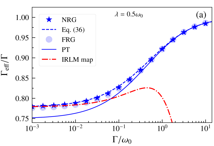
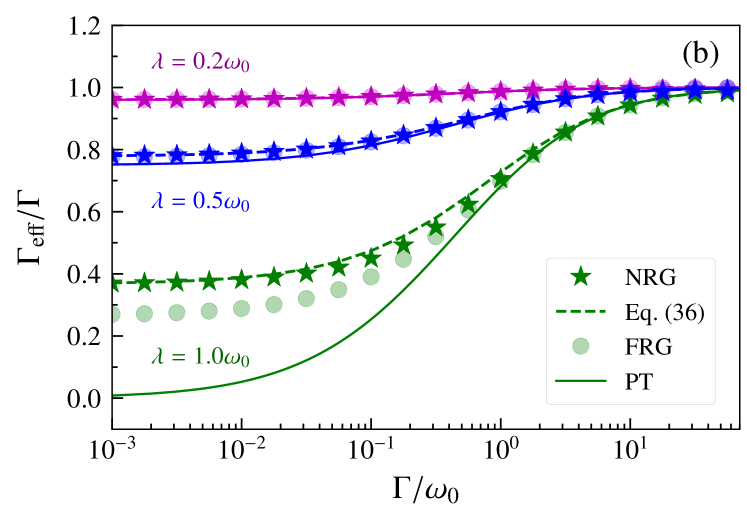
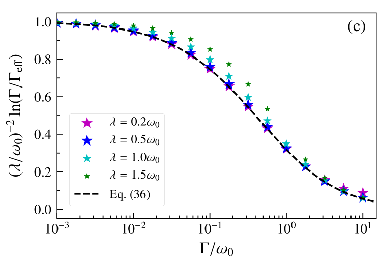
Figure 1: (a) and (b): The ratio of the effective tunneling rate $\Gamma_{\rm eff}$ to the bare value $\Gamma$ as a function of ${\Gamma}/{\omega_{0}}$ using different approaches. (c) The ratio $\big{(}{\lambda}/{\omega_{0}}\big{)}^{-2}\ln\Big{(}{\Gamma_{\rm eff}}/{\Gamma}\Big{)}$ as a function of $\Gamma/\omega_{0}$ for different electron-phonon couplings computed within NRG.

The phonon-assisted suppression of tunneling processes depends on the strength of the electron-phonon coupling, as it is shown in Fig. 1 (b). As we approach the strong coupling regime $\lambda>\omega_{0}$, higher order coefficients in the Taylor expansion of the self-energy feedback in Eq. (25) produce sizable contributions. Therefore the solution of the first order truncated FRG Eq. (23) becomes different from the approximated formula Eq. (38), which was obtained by including the linear coefficient $\gamma_{1}$ only. The approximated formula matches better with the NRG data as compared to the results obtained from the numerical solution of the full lowest order truncated FRG for $\lambda\approx\omega_{0}$ which, however, must be regarded as accidental.

Figure 1 (c) shows that also the NRG data for $\Gamma_{\rm eff}$ approximately follow a scaling form as it is exactly fulfilled in the approximate (in $\lambda^{2}$) expression Eq. (38); $\big{(}\frac{\lambda}{\omega_{0}}\big{)}^{-2}\ln\Big{(}\frac{\Gamma_{\rm eff}^{\rm FRG}}{\Gamma}\Big{)}$ is only a function of $\frac{\omega_{0}}{\Gamma}$. This seems to be valid even for $\lambda\gtrapprox\omega_{0}$ as long as we stay away from the crossover regime between antiadiabatic and adiabatic; in this the exact solution and thus the highly accurate NRG approximation to the latter contains $\lambda/\omega_{0}$ dependent corrections to the simple scaling form. This insight is consistent to the earlier study,Eidelstein et al. (2013) where it was found that in the strong coupling regime the aforementioned ratio is a function of ${E_{\rm p}}/{\Gamma}$.

We address the two extreme antiadiabatic and adiabatic regimes separately in Fig. 2. In the adiabatic limit, the slow molecular vibrations cannot change the charge fluctuations significantly; conventional perturbation theory suffices and matches well with other methods [see Fig. 2 (a)]. As we go sufficiently deep into the adiabatic regime, we obtain the well known asymptotic behavior Eq. (31). We note in passing that in Ref. Jovchev and Anders, 2013 the ratio $\Gamma/\omega_{0}$ was not chosen large enough to properly reproduce the simple expression Eq. (31); for the value considered in this work corrections in $\omega_{0}/\Gamma$ as given in Eq. (30) must be kept.

Figure  2 (b) shows that in the antiadiabatic limit, perturbative results start to deviate already for small electron-phonon couplings.

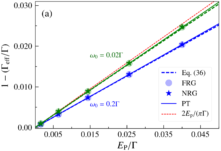
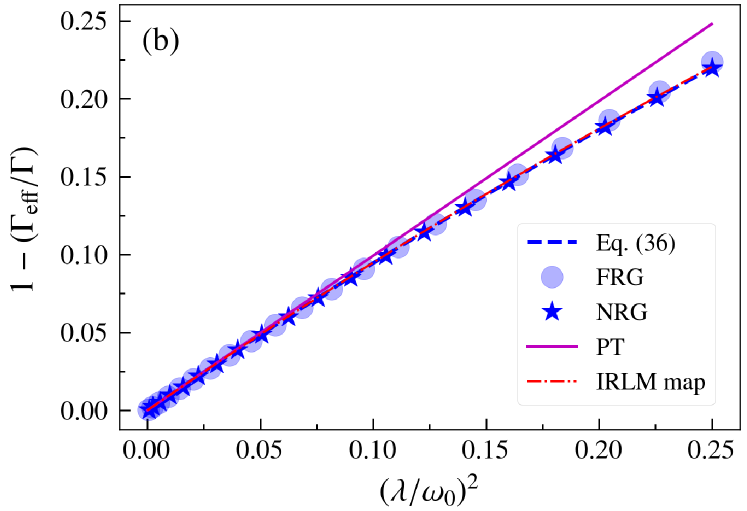
Figure 2: (a) $1-({\Gamma_{\rm eff}}/{\Gamma})$ as a function of ${E_{\rm p}}/{\Gamma}$ for $\omega_{0}=0.2\Gamma$ and $\omega_{0}=0.02\Gamma$ (adiabatic limit). (b) $1-({\Gamma_{\rm eff}}/{\Gamma})$ as a function of $\big{(}{\lambda}/{\omega_{0}}\big{)}^{2}$ for $\omega_{0}=10^{3}\Gamma$ (antiadiabatic limit).

The overall physical picture is the following; phonons induce a retarded and attractive fermion-fermion interaction on the dot [see Eq. (10)] and therefore, the tunneling processes from the dot into the leads are suppressed. This suppression is more significant in the antiadiabatic regime, where phonons are quite fast compared to the tunneling processes.

III.3 Gate voltage dependence of the $T=0$ elelctrical conductance

Having investigated within perturbation theory, FRG and NRG the emergent low-energy scale $\Gamma_{\rm eff}$ at particle-hole symmetry, we now turn to the case of finite particle-hole asymmetry and investigate how this scale manifests itself in the gate voltage dependence of the $T=0$ electrical conductance, making comparisons between the different approaches.

Within the FRG approach, as formulated here in Matsubara space, one would need to analytically continue the molecular dot Green function to the real axis in order to calculate the linear conductance from the molecular spectral functionMeir and Wingreen (1992) as it is often done. This analytic continuation is an ill-posed problem. We can, however, compute the linear conductance as a function of the (bare) level position from the FRG self-energy data without performing the analytic continuation by employing a continued fraction (CF) representation of the Fermi function $f$

$$f(\beta\nu)=\frac{1}{2}-\frac{1}{\beta}\sum_{p=1}^{M}\left\{\frac{R_{p}}{\nu-i\frac{z_{p}}{\beta}}+\frac{R_{p}}{\nu+i\frac{z_{p}}{\beta}}\right\}$$ (42)

at inverse temperature $\beta$. Here the $M$ poles $\frac{z_{p}}{\beta}$ and residues $R_{p}$ can be calculated as proposed in Refs. Ozaki, 2007; Karrasch et al., 2010b. The poles are concentrated densely close to the real axis and they are further apart as we go up and down the imaginary axis. This leads to a very fast convergence of the sum in Eq. (42) as compared to the Matsubara representation. To obtain the conductance at vanishing temperature we choose a sufficiently small $\beta^{-1}=10^{-4}\Gamma^{\rm FRG}_{\rm eff}$. Employing the above mentioned relation between the molecular spectral function $A(\nu)$ and the linear conductance $G$Meir and Wingreen (1992) we obtain

$$\frac{G}{G_{0}} =-\pi\Gamma\int_{-\infty}^{\infty}d\nu A(\nu)\partial_{\nu}f(\beta\nu)$$

$$=\frac{2\pi\Gamma}{\beta}\sum_{\rm p=1}^{M}R_{p}\mbox{Im}\left[\frac{dG_{\rm mol}(i\frac{z_{p}}{\beta})}{d(\frac{z_{p}}{\beta})}\right],$$ (43)

where $G_{0}=e^{2}/h$, with $e$ and $h$ denoting electric charge and Plank’s constant respectively.

To test the CF approach in the present context in Fig. 3 we compare the linear conductance obtained from the self-energy in lowest order perturbation theory after performing the analytic continuation as in Eq. (17) [using the first line of Eq. (43)] (dashed line) and the continued fraction representation employing Matsubara frequency data as in Eqs. (14) and (15) [using the last line of Eq. (43)] (plus signs). Both conductance curves agree well. For the weak interaction of this figure, and on the scale of the plot, perturbation theory matches the FRG data (obtained from the continued fraction representation; circles) as well as the NRG ones (stars). The latter were obtained from the spectral weight $A(\nu=0)$ [see the $T=0$ limit of the first line of Eq. (43)]. Due to the presence of phonons, the linear conductance is narrower as compared to the noninteracting case. This effect can be captured within perturbation theory as long as ${E_{\rm p}}/{\Gamma}<{\pi}/{2}$. Therefore, if we are deep in the antiadiabatic limit, perturbation theory is limited to extremely small coupling constants $\lambda/\omega_{0}$.

Figure 3: Comparison of the different approaches to compute the $T=0$ linear conductance as a function of the gate voltage $\epsilon_{0}-E_{\rm p}$ for a given phonon frequency $\omega_{0}=2\Gamma$ in the weak coupling regime ($\lambda=0.5\omega_{0}$).

Figure 4 shows that FRG results for $G$ match very well to the NRG data for $\lambda/\omega_{0}\lessapprox 1$. The narrowing of the linear conductance reflects that due to molecular vibrations, small misalignment of the gate voltage to the chemical potential of the leads can result in a substantial drop in transport. This is just another indication of the suppression of tunneling processes. In fact, if we rescale the level position with the renormalized tunneling rate $\Gamma_{\rm eff}$, all the NRG curves corresponding to different strengths of electron-phonon coupling collapse, with good accuracy, to the noninteracting curve as shown in the inset of Fig. 4. This shows that $\Gamma_{\rm eff}$ is the relevant low-energy scale also away from particle-hole symmetry; the width of the linear conductance resonance as a function of the level position is given by $\Gamma_{\rm eff}$.

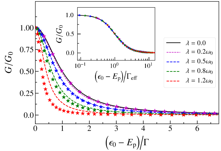
Figure 4: Comparison of FRG (dashed lines) and NRG (stars) results for the zero temperature linear conductance as a function of the gate voltage $\epsilon_{0}-E_{\rm p}$ for different strength of electron-phonon couplings in the antiadiabatic limit ($\omega_{0}=10^{3}\Gamma$). The inset shows the zero temperature conductance from NRG as a function of the rescaled gate voltage $({\epsilon_{0}-E_{\rm p}})/{\Gamma_{\rm eff}}$ for different strength of the electron-phonon coupling in the antiadiabatic limit ($\omega_{0}=10^{3}\Gamma$).

IV Summary and outlook

Using a combination of lowest order perturbation theory, (truncated) FRG, and NRG we studied phonon assisted tunneling in an elementary model of a molecular electronics device. Complementing an earlier strong coupling studyEidelstein et al. (2013) our focus was on weak to intermediate electron-phonon coupling. We derived an analytic expression for the renormalized tunnel coupling at particle-hole symmetry valid for all ratios $\Gamma/\omega_{0}$ from the antiadiabatic into the adiabatic regime. It captures the combined exponential (polaronic) and power-law (x-ray edge singularity) renormalization in the antiadiabatic limit known from the mapping to an effective IRLM. Away from particle-hole symmetry we investigated the influence of the emergent low-energy scale $\Gamma_{\rm eff}$ on the $T=0$ electrical conductance, comparing also the results within different approaches.

In a follow-up paper,Khedri et al. (2017) we consider a (small) temperature bias as the driving force and in this way extend our study to linear thermoelectric properties of molecular devices. Such devices are considered to be promising building blocks for waste heat conversion and cooling on the molecular level.Mahan et al. (1997); Giazotto et al. (2006) Indeed, in Ref. Khedri et al., 2017, employing the NRG,Costi and Zlatić (2010) we find parameter regimes where the linear thermoelectric response through such a device is significantly enhanced.

In the near future we plan to further extend the FRG to the Keldysh contourJakobs et al. (2007); Karrasch et al. (2010a); Laakso et al. (2014) in order to compute the equilibrium spectral function without the need for an analytic continuation. This will in addition enable us to investigate the nonlinear (finite voltage and temperature bias) thermoelectric transport properties of molecular devices described by the SAHM.

Appendix A Numerical implementation of the flow equations

To solve the coupled differential Eqs. (11) and (12), first we discretize the Mathsubara frequency. In the light of the emergent low-energy scale, we use the following logarithmic grid to resolve the low-frequency regime better

$$\nu_{k}=\Delta\frac{2k-N_{\rm tot}}{N_{\rm tot}}\exp\Bigg{\{}\frac{|N_{\rm tot}-2k|-N_{\rm tot}}{S}\Bigg{\}},$$ (44)

with $k=0,1,\cdots N_{\rm tot}$. It distributes $N_{\rm tot}+1$ frequencies symmetrically around zero (Fermi-level) in interval $[-\Delta,\Delta]$. With parameter $S$, we can control the concentration of points around zero. We choose the parameters such that the desired convergence ($10^{-10}$ in units of $\omega_{0}$) is achieved. Linear interpolation is used to evaluate the feedbacks $\epsilon^{\Lambda}(i\Lambda)$ and $\gamma^{\Lambda}(i\Lambda)$ on the right-hand side of Eqs. (11) and (12). The set of $2(N_{\rm tot}+1)$ differential equations can then be solved using standard adaptive routines.

Appendix B Phonon parameters

The minimum number of phonons required to resolve the low-energy behavior of the system depends on the strength of the electron-phonon coupling. Figure 5 shows the convergence of the effective tunneling rate with the number of phonons retained. We used $N_{b}=40$ phonons throughout, which suffices to obtain converged results for all parameters used.

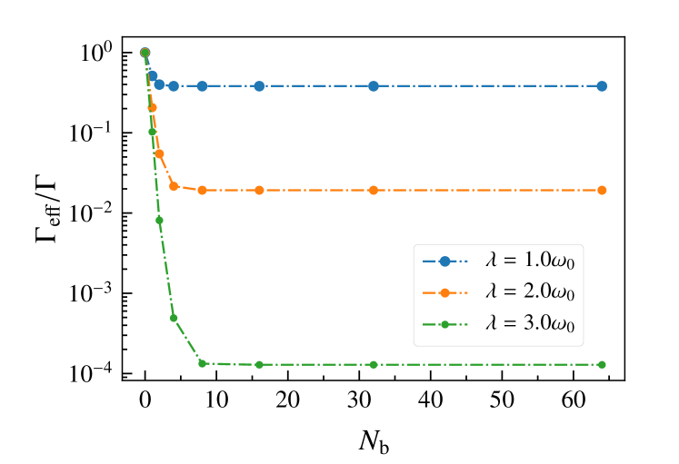
Figure 5: The ratio of the effective tunneling rate $\Gamma_{\rm eff}$ to the bare value $\Gamma$ as a function of $N_{b}$ for different electron-phonon couplings in the antiadiabatic limit ($\omega_{0}=100\Gamma$).

Appendix C NRG and perturbation theory comparisons for the $T=0$ spectral function

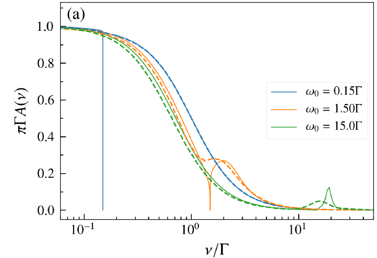
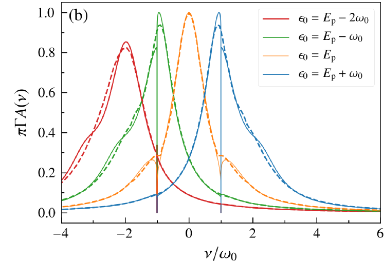
Figure 6: Comparison of the molecular spectral function obtained from perturbation theory (solid lines) and NRG (dashed lines). (a) shows the spectral function at the particle-hole symmetric point $\epsilon_{0}=E_{\rm p}$ for different $\Gamma/\omega_{0}$ at a fixed electron-phonon coupling $\lambda=0.7\omega_{0}$ as a function of $\nu/\Gamma$. Note the logarithmic x-axis scale. (b) depicts the spectral function at different gate voltages for $\omega_{0}=1.5\Gamma$ and $\lambda=0.5\omega_{0}$ as a function of $\nu/\omega_{0}$.

In the FRG approach, as formulated here, we have access to the propagator of the molecular level only in Matsubara space and hence in order to obtain its spectral function, we have to perform an analytic continuation to the real axis; this constitutes an ill-posed problem. It becomes an obstacle as the self-energy at the end of the RG flow is known only numerically. This problem was avoided in the calculation of the conductance in Sec. III.3 by using a continued fraction expansion of the Fermi function. While we can obtain results for spectral functions within FRG by performing the analytic continuation numerically via a Páde approximation, we found this to be a quite unstable procedure in the sense that the results strongly depend on the number of data points and the frequency grid. An alternative, avoiding analytic continuation altogether, which we plan to follow in the future, is to use FRG within the Keldysch formalism, which would also allow accessing nonequilibrium.Jakobs et al. (2007); Karrasch et al. (2010a); Laakso et al. (2014) In order, nevertheless, to compare our results for NRG spectral functions with another method, we show here comparisons to lowest order perturbation theory.

Figure 6 (a) shows the comparison of the spectral function computed within NRG and perturbation theory at particle-hole symmetry as we go from the adiabatic limit to the antiadiabatic one. We see that the central peak gets narrower, reflecting the suppression of tunneling processes. In addition, distinctive satellite peaks at multiples of $\omega_{0}$ start to form. In the antiadiabatic limit, the width of the spectral function calculated from the two approaches do not quite match in agreement to our previous discussion of the effective tunneling coupling $\Gamma_{\rm eff}$ [see Fig. 2 (b)].

As discussed in connection with Eq. (17) the perturbative retarded self-energy shows spurious logarithmic divergencies as $\nu=\pm\omega_{0}$. These lead to zeros of the spectral function which manifest as rather sharp dips in Fig. 6. These sharp features are artifacts of the perturbation theory and are absent in the NRG results. Similar artifacts of perturbation theory were found for the spinful Anderson-Holstein model by comparison to spectral functions obtained from Keldysh FRG (in equilibrium).Laakso et al. (2014) For $\epsilon_{0}>E_{\rm p}$ ($\epsilon_{0}<E_{\rm p}$) the central peak, located at $\nu=0$ for particle-hole symmetry, is shifted to the right (left). This effect is captured rather accurately by perturbation theory for ${E_{\rm p}}/{\Gamma}<{\pi}/{2}$ [Fig. 6 (b)].

References

- Mahan (2000) G. Mahan, Many-Particle Physics (Springer US, Boston, MA, 2000).
- Mitra et al. (2004) A. Mitra, I. Aleiner, and A. J. Millis, Phys. Rev. B 69, 245302 (2004).
- Sherrington and von Molnàr (1975) D. Sherrington and S. von Molnàr, Solid State Communications 16, 1347 (1975).
- Hewson and Newns (1979) A. C. Hewson and D. M. Newns, Journal of Physics C: Solid State Physics 12, 1665 (1979).
- Hewson and Newns (1980) A. C. Hewson and D. M. Newns, Journal of Physics C: Solid State Physics 13, 4477 (1980).
- Hewson and Meyer (2002) A. C. Hewson and D. Meyer, Journal of Physics: Condensed Matter 14, 427 (2002).
- Cornaglia et al. (2004) P. S. Cornaglia, H. Ness, and D. R. Grempel, Phys. Rev. Lett. 93, 147201 (2004).
- Paaske and Flensberg (2005) J. Paaske and K. Flensberg, Phys. Rev. Lett. 94, 176801 (2005).
- Galperin et al. (2007) M. Galperin, M. A. Ratner, and A. Nitzan, Journal of Physics: Condensed Matter 19, 103201 (2007).
- Hyldgaard et al. (1994) P. Hyldgaard, S. Hershfield, J. Davies, and J. Wilkins, Annals of Physics 236, 1 (1994).
- König et al. (1996) J. König, J. Schmid, H. Schoeller, and G. Schön, Phys. Rev. B 54, 16820 (1996).
- Braig and Flensberg (2003) S. Braig and K. Flensberg, Phys. Rev. B 68, 205324 (2003).
- Koch and von Oppen (2005) J. Koch and F. von Oppen, Phys. Rev. Lett. 94, 206804 (2005).
- Han (2006) J. E. Han, Phys. Rev. B 73, 125319 (2006).
- Han (2010) J. E. Han, Phys. Rev. B 81, 113106 (2010).
- Mühlbacher and Rabani (2008) L. Mühlbacher and E. Rabani, Phys. Rev. Lett. 100, 176403 (2008).
- Schiró and Fabrizio (2009) M. Schiró and M. Fabrizio, Phys. Rev. B 79, 153302 (2009).
- Koch et al. (2011) T. Koch, J. Loos, A. Alvermann, and H. Fehske, Phys. Rev. B 84, 125131 (2011).
- Hützen et al. (2012) R. Hützen, S. Weiss, M. Thorwart, and R. Egger, Phys. Rev. B 85, 121408 (2012).
- Jovchev and Anders (2013) A. Jovchev and F. B. Anders, Phys. Rev. B 87, 195112 (2013).
- Roura-Bas et al. (2013) P. Roura-Bas, L. Tosi, and A. A. Aligia, Phys. Rev. B 87, 195136 (2013).
- Laakso et al. (2014) M. A. Laakso, D. M. Kennes, S. G. Jakobs, and V. Meden, New Journal of Physics 16, 023007 (2014).
- Albrecht et al. (2013) K. F. Albrecht, A. Martin-Rodero, R. C. Monreal, L. Mühlbacher, and A. Levy Yeyati, Phys. Rev. B 87, 085127 (2013).
- Leturcq et al. (2009) R. Leturcq, C. Stampfer, K. Inderbitzin, L. Durrer, C. Hierold, E. Mariani, M. G. Schultz, F. von Oppen, and K. Ensslin, Nat Phys 5, 327 (2009).
- Lang and Firsov (1962) I. Lang and Y. Firsov, Zh. Eksp. Teor. Fiz. 43, 1843 (1962), [Sov. Phys.-JETP 16, 1301 (1963)].
- Eidelstein et al. (2013) E. Eidelstein, D. Goberman, and A. Schiller, Phys. Rev. B 87, 075319 (2013).
- Schlottmann (1980) P. Schlottmann, Phys. Rev. B 22, 613 (1980).
- Schlottmann (1982) P. Schlottmann, Phys. Rev. B 25, 4815 (1982).
- Khedri et al. (2017) A. Khedri, V. Meden, and T. A. Costi, Phys. Rev. B 96, 195156 (2017).
- Metzner et al. (2012) W. Metzner, M. Salmhofer, C. Honerkamp, V. Meden, and K. Schönhammer, Rev. Mod. Phys. 84, 299 (2012).
- Karrasch et al. (2010a) C. Karrasch, M. Pletyukhov, L. Borda, and V. Meden, Phys. Rev. B 81, 125122 (2010a).
- Karrasch et al. (2006) C. Karrasch, T. Enss, and V. Meden, Phys. Rev. B 73, 235337 (2006).
- Kennes (2014) D. M. Kennes, Ph.D. thesis, RWTH Aachen University (2014).
- Campo and Oliveira (2005) V. L. Campo and L. N. Oliveira, Phys. Rev. B 72, 104432 (2005).
- Wilson (1975) K. G. Wilson, Rev. Mod. Phys. 47, 773 (1975).
- Krishna-murthy et al. (1980) H. R. Krishna-murthy, J. W. Wilkins, and K. G. Wilson, Phys. Rev. B 21, 1003 (1980).
- Bulla et al. (2008) R. Bulla, T. A. Costi, and T. Pruschke, Rev. Mod. Phys. 80, 395 (2008).
- Ingersent (2015) K. Ingersent, in Many-Body Physics: From Kondo to Hubbard, Modeling and Simulation, Vol. 5, edited by E. Pavarini, E. Koch, and P. Coleman (Forschungszentrum Jülich GmbH Zentralbibliothek, Verlag, Jülich, 2015) Chap. 6.
- Bulla et al. (1998) R. Bulla, A. C. Hewson, and T. Pruschke, Journal of Physics: Condensed Matter 10, 8365 (1998).
- Vinkler et al. (2012) Y. Vinkler, A. Schiller, and N. Andrei, Phys. Rev. B 85, 035411 (2012).
- Meir and Wingreen (1992) Y. Meir and N. S. Wingreen, Phys. Rev. Lett. 68, 2512 (1992).
- Ozaki (2007) T. Ozaki, Phys. Rev. B 75, 035123 (2007).
- Karrasch et al. (2010b) C. Karrasch, V. Meden, and K. Schönhammer, Phys. Rev. B 82, 125114 (2010b).
- Mahan et al. (1997) G. Mahan, B. Sales, and J. Sharp, Phys. Today 50, 42 (1997).
- Giazotto et al. (2006) F. Giazotto, T. T. Heikkilä, A. Luukanen, A. M. Savin, and J. P. Pekola, Rev. Mod. Phys. 78, 217 (2006).
- Costi and Zlatić (2010) T. A. Costi and V. Zlatić, Phys. Rev. B 81, 235127 (2010).
- Jakobs et al. (2007) S. G. Jakobs, V. Meden, and H. Schoeller, Phys. Rev. Lett. 99, 150603 (2007).