A Curious Family of Binomial Determinants That Count Rhombus Tilings of a Holey Hexagon

Abstract

We evaluate a curious determinant, first mentioned by George Andrews in 1980 in the context of descending plane partitions. Our strategy is to combine the famous Desnanot-Jacobi-Dodgson identity with automated proof techniques. More precisely, we follow the holonomic ansatz that was proposed by Doron Zeilberger in 2007. We derive a compact and nice formula for Andrews’s determinant, and use it to solve a challenge problem that we posed in a previous paper. By noting that Andrews’s determinant is a special case of a two-parameter family of determinants, we find closed forms for several one-parameter subfamilies. The interest in these determinants arises because they count cyclically symmetric rhombus tilings of a hexagon with several triangular holes inside.

1 Introduction

Plane partitions were a hot topic back in the 1970’s and 1980’s (as beautifully described in [4]), and they still keep combinatorialists busy. For example, the $q$-enumeration formula of totally symmetric plane partitions, conjectured independently by David Robbins and George Andrews in 1983, remained open for almost 30 years and was finally proved in 2011 [8] using massive computer algebra calculations. The problem that we treat in this paper originates around the same time, when combinatorialists started to employ determinants to reformulate the counting problem of plane partitions.

The following determinant counts descending plane partitions, and it was famously evaluated by George Andrews [2] in 1979:

$$\det_{1\leqslant i,j\leqslant n}\left(\delta_{i,j}+\binom{\mu+i+j-2}{j-1}\right),$$ (1.1)

where $\delta_{i,j}$ denotes the Kronecker delta, i.e., $\delta_{i,j}=1$ if $i=j$ and $\delta_{i,j}=0$ otherwise. The same determinant is also mentioned in Krattenthaler’s classic treatise on determinants [11, Thm. 32] (where $\mu$ is replaced by $2\mu$). One year later, in 1980, Andrews [3, page 105] came up with a curious determinant which is a slight variation of the above:

$$D(n):=\det_{1\leqslant i,j\leqslant n}\left(\delta_{i,j}+{\binom{\mu+i+j-2}{j}}\right).$$

He conjectured a closed-form formula for the quotient $D(2n)/D(2n-1)$. It was mentioned again (and popularized) as Problem 34 in Krattenthaler’s complement [12], and it was proven, for the first time, by the authors of the present paper in 2013 [9].

However this proves only “half” of the formula for $D(n)$. The quotient $D(2n+1)/D(2n)$ remained mysterious, due to an increasingly large “ugly” (i.e., irreducible) polynomial factor that is always shared between two consecutive determinants. Thus the determinant $D(n)$ does not completely factor into linear polynomials, while many similar determinants do. Not fully satisfied with this situation, the first-named author made a monstrous conjecture [9, Conj. 6] of the full formula for $D(n)$. In this paper, we derive and prove a nicer formula for $D(n)$ (Section 4) and also show that it is equivalent to our previous conjecture (Section 5). In order to obtain the nice formula for $D(n)$, we have to evaluate some related determinants (Section 3), which we then combine via the Desnanot-Jacobi-Dodgson identity. In Section 6, we identify these determinants as special cases of some more general (infinite) families of determinants and present several theorems and conjectures for their closed forms. All of them have a combinatorial meaning, as will be explained in Section 2. We first introduce the main object of study of this article, the generalized determinant with shifted corner:

Definition 1.

For $n,s,t\in\mathbbm{Z}$, $n\geqslant 1$, and $\mu$ an indeterminate, we define $D_{s,t}(n)$ to be the following $(n\times n)$-determinant:

$$D_{s,t}(n)\mathrel{\mathop{:}}=\det_{\genfrac{}{}{0.0pt}{}{s\leqslant i<s+n}{t\leqslant j<t+n}}\left(\delta_{ij}+{\binom{\mu+i+j-2}{j}}\right),\qquad n\geqslant 1.$$

Note that Andrews’s determinant is a special case of it, namely $D(n)=D_{1,1}(n)$, and that (1.1) equals $D_{0,0}(n)$ after replacing $\mu$ by $\mu+2$.

Notation.

We employ the usual notation $(x)_{k}$ for the Pochhammer symbol (also known as rising factorial), that is defined as follows:

$$(x)_{k}\mathrel{\mathop{:}}=\begin{cases}x(x+1)\cdots(x+k-1),&k>0,\\ 1,&k=0,\\ \frac{1}{(x+k)_{-k}},&k<0.\end{cases}$$

The short-hand notation $(x)_{k}^{2}$ is to be interpreted as $\bigl{(}(x)_{k}\bigr{)}^{2}$. The double factorial is defined, as usual, as

$$n!!\mathrel{\mathop{:}}=\begin{cases}2\cdot 4\cdots(n-2)\cdot n,&\text{if $n$ is even,}\\ 1\cdot 3\cdots(n-2)\cdot n,&\text{if $n$ is odd.}\end{cases}$$

2 Combinatorial Background

Before we go into details about the evaluations of the mentioned determinant $D_{1,1}(n)$, and more generally $D_{s,t}(n)$, we want to give a combinatorial interpretation of these determinants, namely we exhibit certain combinatorial objects (rhombus tilings) that are counted by them.

The determinant $D_{0,0}(n)$, which is given in (1.1), was evaluated by George Andrews [2], because it counts descending plane partitions. Christian Krattenthaler [13] observed that it equivalently counts cyclically symmetric rhombus tilings of a hexagon with a triangular hole, where the size of the hole is related to the parameter $\mu$ [5, Thm. 6]. From this, we deduce that our generalized version can count similar objects. Throughout this section, we use the transformed parameter $\lambda:=\mu-2$, which turns out to be more natural in this context (compare also with Andrews’ paper [2]).

The first observation is that $D_{s,t}(n)$ can be written as a sum of minors. For this purpose, we rewrite it by performing index shifts on $i$ and $j$:

$$D_{s,t}(n)=\det_{\genfrac{}{}{0.0pt}{}{s\leqslant i<s+n}{t\leqslant j<t+n}}\left(\delta_{ij}+{\binom{\lambda+i+j}{j}}\right)=\det_{\genfrac{}{}{0.0pt}{}{1\leqslant i\leqslant n}{1\leqslant j\leqslant n}}\left(\delta_{i+s-t,j}+{\binom{\lambda+i+j+s+t-2}{j+t-1}}\right).$$

For the sake of readability, we abbreviate the latter binomial coefficient by $b_{i,j}$, and do not denote the dependency on $s$ and $t$. Let $i\in\{1,\dots,n\}$ be such that $1\leqslant i+s-t\leqslant n$, i.e. the $i$-th row contains one entry where the Kronecker delta evaluates to $1$, then by Laplace expansion with respect to the $i$-th row one obtains

$$D_{s,t}(n)=\det_{\genfrac{}{}{0.0pt}{}{1\leqslant i\leqslant n}{1\leqslant j\leqslant n}}\bigl{(}\delta_{i+s-t,j}+b_{i,j}\bigr{)}=\sum_{j=1}^{n}(-1)^{j+1}\bigl{(}\delta_{i+s-t,j}+b_{i,j}\bigr{)}M^{i}_{j}=(-1)^{s-t}M^{i}_{i+s-t}+\sum_{j=1}^{n}(-1)^{i+j}b_{i,j}M^{i}_{j},$$

where $M^{i}_{j}$ denotes the $(i,j)$-minor of the corresponding matrix. More generally, for any matrix $A$, we can write $\det(A)=\det(A^{-})+(-1)^{i+j}M^{i}_{j}$, where $A^{-}$ denotes the matrix $A$ after subtracting $1$ from its $(i,j)$-entry. Applying this formula recursively to the determinant $D_{s,t}(n)$, until all $1$’s coming from the Kronecker deltas are eliminated, yields the following identity

$$D_{s,t}(n)=\begin{cases}\displaystyle\sum_{I\subseteq\{1,\dots,n-s+t\}}(-1)^{(s-t)\cdot|I|}\cdot\det\bigl{(}B^{I}_{I+s-t}\bigr{)},&\text{if }s\geqslant t,\\ \displaystyle\sum_{I\subseteq\{1,\dots,n-t+s\}}(-1)^{(s-t)\cdot|I|}\cdot\det\bigl{(}B^{I+t-s}_{I}\bigr{)},&\text{if }s\leqslant t,\rule{0.0pt}{20.0pt}\end{cases}$$ (2.1)

where $I+x=\{i+x\mid i\in I\}$ and where $B^{I}_{J}$ denotes the matrix that is obtained by deleting all rows with indices in $I$ and all columns with indices in $J$ from the matrix $B_{s,t}(n)=(b_{i,j})_{1\leqslant i,j\leqslant n}$. In other words, we are summing over all subsets of positions where the Kronecker delta evaluates to $1$, and for each such subset we add or subtract the corresponding minor $\det\bigl{(}B^{I}_{J}\bigr{)}$.

The second observation is that, by the Lindström–Gessel–Viennot lemma [14, 6], $\det\bigl{(}B_{s,t}(n)\bigr{)}$ counts $n$-tuples of non-intersecting paths in the integer lattice $\mathbbm{N}^{2}$: the start points are $(\lambda+s,0)$, $(\lambda+s+1,0)$, …, $(\lambda+s+n-1,0)$, the end points are $(0,t),(0,t+1),\dots,(0,t+n-1)$, and the allowed steps are $(0,1)$ and $(-1,0)$; see Figure 1 (left) for an example. The number of paths starting at $(\lambda+s+i-1,0)$ and ending at $(0,t+j-1)$ is given by $\binom{\lambda+i+j+s+t-2}{j+t-1}$, which is precisely the $(i,j)$-entry of $B_{s,t}(n)$. Note that this counting is only correct if $\lambda+s\geqslant 0$; in the following we will assume that this condition is satisfied. We do not know of a combinatorial interpretation when $\lambda+s<0$.

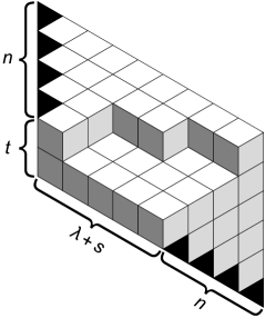
Figure 1: A tuple of non-intersecting lattice paths (for $n=4$, $t=2$, and $\lambda+s=5$), and the corresponding rhombus tiling of a lozenge with some missing triangles (black): the white rhombi correspond to left-steps and the light-gray rhombi correspond to up-steps.

If $|I|=|J|$ then $\det\bigl{(}B^{I}_{J}\bigr{)}$ counts the $(n-|I|)$-tuples of non-intersecting paths where the start points with indices $I$ and the end points with indices $J$ are omitted. In the case $s=t$, the expression $\sum_{I\subseteq\{1,\dots,n\}}\det\bigl{(}B^{I}_{I}\bigr{)}$ counts all tuples of non-intersecting paths for all subsets of start points (and the same subset of end points). If $s>t$ then we use $\det\bigl{(}B^{I}_{I+s-t}\bigr{)}$ with $I\subseteq\{1,\dots,n-s+t\}$. This means that we never omit the last $s-t$ start points on the horizontal axis and we never omit the first $s-t$ end points on the vertical axis (counted from bottom to top). Moreover, the omitted start and end points follow the same pattern, shifted by $s-t$. If $t>s$ then we never omit the first $t-s$ start points and the last $t-s$ end points.

The third and final observation is that the previously described non-intersecting lattice paths are in bijection with rhombus tilings of a lozenge-shaped region, where certain triangles on the border are cut out. They correspond to the start and end points; see the right part of Figure 1 where these triangles are colored black. The two types of steps (left and up) correspond to two orientations of the rhombi (colored white and light-gray), while rhombi of the third possible orientation (colored dark-gray) fill the areas which are not covered by paths. From Figure 1 it is apparent that the lozenge has width $\lambda+n+s$ and height $n+t$, and that $n$ black triangles are placed at the right end of its lower side and another $n$ black triangles at the top of its left vertical side. From the bijection with lattice paths we see that the number of rhombus tilings of such a lozenge is given by the determinant $\det\bigl{(}B_{s,t}(n)\bigr{)}$.

In order to give a combinatorial interpretation to the determinant $D_{s,t}(n)$, we have to sum up the counts of many similar tiling problems, according to the sum of minors (2.1). More precisely, label the black triangles on the lower side of the lozenge with numbers from $1$ to $n$ (from left to right), and similarly those on the vertical side (from bottom to top). Then $\det\bigl{(}B^{I}_{J}\bigr{)}$ counts rhombus tilings of the lozenge where all black triangles on the lower side with labels in $I$ are removed, and similarly, all black triangles on the vertical side with labels in $J$. Instead of adding up the results of many counting problems, we can elegantly obtain the same result from a single counting problem, by introducing cyclically symmetric rhombus tilings of hexagonal regions.

For this purpose, we rotate the lozenge by $120^{\circ}$ and by $240^{\circ}$ and put the three copies together such that corresponding triangles share an edge. We illustrate this procedure in Figure 2: on the left we show the three copies of the lozenge from Figure 1 with parameters $s=4$, $t=2$, $n=4$, and $\lambda=2$. Since $s-t=2$ we never omit the last two start points and the first two end points. Therefore, the corresponding triangles are colored black. The fact that the remaining start and end points may be omitted, is indicated by lighter colors. The relation between $I$ and $J=I+s-t$ is visualized by matching colors: for two triangles of the same color we have that either both are present or both are omitted. The three copies of the lozenge are glued together such that triangles of the same color share an edge. Note that this implies that none of the black triangles will have a partner.

    

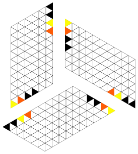
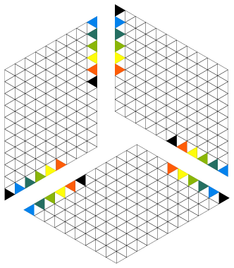
Figure 2: Gluing together three copies of a lozenge; the left figure corresponds to the parameters $s=4$, $t=2$, $n=4$, $\lambda=2$, while the right figure has $s=2$, $t=3$, $n=6$, $\lambda=3$

Now we obtain a region that is either a hexagon (if $s=t$) or that otherwise has the shape of a pinwheel; see Figure 3. In both cases, there remains a “hole” in the center, except when $\lambda=0$. If $\lambda\neq 0$ then this hole has the shape of an equilateral triangle of side length $|\lambda|$, pointing to the right if $\lambda>0$ and pointing to the left if $\lambda<0$. We have to ensure that no rhombus crosses the border of the original lozenge except for those positions that correspond to the start and end points of the paths. For this reason, we place a “border line” of length $\min(s,t)$ at each corner of the triangular hole and prohibit any rhombus to lie across this border. Note that in the case $\lambda<0$ the vertical border actually starts at the lower vertex of the (left pointing) triangular hole, so that $\min(s,t,-\lambda)$ unit segments of the border coincide with the right side of the triangular hole (and similarly for the other two border lines). Each of these border lines is continued by $|s-t|$ unit triangular holes that point either in clockwise direction (if $s>t$) or in counter-clockwise direction (if $s<t$). The same number of triangles appears at the “wings” of the pinwheel, at a distance of $n-|s-t|$ from the end of the border line; these triangles point in the opposite direction.

Since we have now three copies of the original domain, we have to avoid overcounting: this is done by restricting the count to rhombus tilings that are cyclically symmetric. At the same time this restriction automatically ensures that the relation between start and end points is satisfied, namely that they are distributed in the same manner, only shifted by $|s-t|$, as described before.

By construction, we have obtained a region whose cyclically symmetric rhombus tilings are counted by the determinant $D_{s,t}(n)$, provided that $s-t$ is even. If $s-t$ is odd, the count is weighted by $+1$ and $-1$: the sign is determined by the parity of the number of rhombi crossing the original vertical side of the lozenge. Recall that the sign comes from $(-1)^{(s-t)\cdot|I|}$ in (2.1). The cardinality $|I|$ corresponds to the number of vertical line segments between the two vertical strips of black triangles that are “visible”, i.e., that are not covered by a horizontal rhombus. In other words: if there is an even number of line segments that are not crossed by a horizontal rhombus then the count is weighted with $+1$, otherwise with $-1$. By a “horizontal rhombus” we mean one that is built of two triangles sharing a vertical edge.

Figure 3: Pinwheel-shaped regions with holes: the left figure corresponds to the parameters $s=5$, $t=1$, $n=5$, $\lambda=2$, the right figure corresponds to $s=2$, $t=3$, $n=6$, $\lambda=3$ (same as in Figure 2).

The construction can be simplified by noting that a row of small triangular holes induces a unique rhombus tiling when completing it to a big equilateral triangle. Hence the pinwheel-shaped region can be replaced by a hexagon, by cutting off three equilateral triangles of size $|s-t|$, without changing the number of rhombus tilings. Similarly, the holes inside the region can be re-interpreted as four triangular holes, of size $|\lambda|$ resp. $|s-t|$, that are connected by boundary lines. We give an illustration of these regions in Figure 4.

Figure 4: Hexagonal regions with big triangular holes and border lines: the left figure corresponds to the same parameters as in Figure 3 ($s=5$, $t=1$, $n=5$, $\lambda=2$), the right figure corresponds to $s=-1$, $t=2$, $n=6$, $\lambda=4$.

As an example, we have worked out all cyclically symmetric rhombus tilings of the hexagon that corresponds to $D_{1,1}(2)$ with $\lambda=1$; see Figure 5. In this case, one can easily calculate

$$D_{1,1}(2)\big{|}_{\lambda\to 1}=\begin{vmatrix}4&6\\ 4&11\end{vmatrix}=20.$$

Another example that illustrates our combinatorial construction is the identity

$$D_{s,t}(n)=D_{t+\lambda,s+\lambda}(n)\big{|}_{\lambda\to-\lambda}$$

that follows directly by the mirror symmetry of the underlying tiling regions. Assuming $\lambda\geqslant 0$, the determinant $D_{s,t}(n)$ counts cyclically symmetric rhombus tilings of a hexagon that has a triangular hole of size $\lambda$ pointing to the right, with border lines of length $\min(s,t)$, to each of which another triangular hole of size $|s-t|$ is attached, pointing in clockwise direction if $s>t$. When we consider the transformed parameters $s^{\prime}=t+\lambda$, $t^{\prime}=s+\lambda$, and $\lambda^{\prime}=-\lambda$, we obtain a hexagonal region with a hole of size $|\lambda^{\prime}|=\lambda$ pointing to the left, with border lines of length $\min(s^{\prime},t^{\prime})=\min(s,t)+\lambda$, each of which shares a segment of length $\lambda$ with the hole (so only $\min(s,t)$ units are visible), and with three other triangular holes of size $|s^{\prime}-t^{\prime}|=|s-t|$ each, pointing in counterclockwise direction if $t^{\prime}>s^{\prime}$ (${\iff}$ $s>t$). Thus these two regions are symmetric w.r.t. to a vertical axis and therefore possess the same number of rhombus tilings.

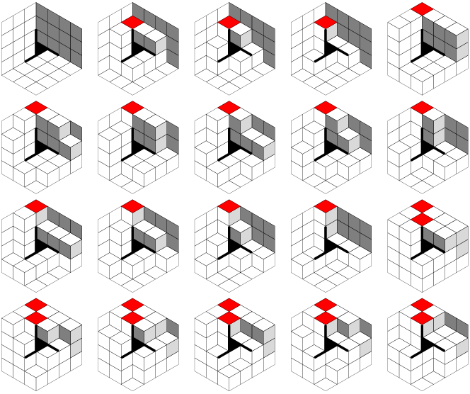
Figure 5: All 20 cyclically symmetric rhombus tilings for the parameters $s=t=1$, $n=2$, and $\lambda=1$. The original lozenge is highlighted by shaded rhombi, the horizontal rhombi marking the end points of the lattice paths are colored red.

3 Related Determinants

In this section, we prove a few easier results about particular instances of the determinant $D_{s,t}(n)$, with specific shifted corners, by using computer proofs. Later, we put all these results together and obtain from it a “closed-form” formula for $D(n)\quad(=D_{1,1}(n))$, via the celebrated Desnanot-Jacobi-Dodgson identity: let $\bigl{(}m_{i,j}\bigr{)}_{i,j\in\mathbbm{Z}}$ be a doubly infinite sequence and denote by $M_{s,t}(n)$ the determinant of the $(n\times n)$-matrix whose upper left entry is at $m_{s,t}$, more precisely the matrix $\bigl{(}m_{i,j}\bigr{)}_{s\leqslant i<s+n,t\leqslant j<t+n}$. Then:

$$M_{s,t}(n)M_{s+1,t+1}(n-2)=M_{s,t}(n-1)M_{s+1,t+1}(n-1)-M_{s+1,t}(n-1)M_{s,t+1}(n-1).$$ (DJD)

For an excellent overview of this topic see [1].

The following result was conjectured in [3], and in 2013 it was proven by the authors of the present paper [9, Thm. 1]:

Theorem 2.

Let the determinant $D_{1,1}(n)$ be as in Definition 1. Then the following equation holds:

$$\frac{D_{1,1}(2n)}{D_{1,1}(2n-1)} =(-1)^{(n-1)(n-2)/2}\,2^{n}\,\frac{\left(\frac{\mu}{2}+2n+\frac{1}{2}\right)_{\!n-1}\left(\frac{\mu}{2}+n\right)_{\!\lfloor(n+1)/2\rfloor}}{\bigl{(}n\bigr{)}_{\!n}\left(-\frac{\mu}{2}-2n+\frac{3}{2}\right)_{\!\lfloor(n-1)/2\rfloor}}$$

$$=2^{n}\,\frac{\left(\frac{\mu}{2}+2n+\frac{1}{2}\right)_{\!n-1}\left(\frac{\mu}{2}+n\right)_{\!\lfloor(n+1)/2\rfloor}}{\bigl{(}n\bigr{)}_{\!n}\left(\frac{\mu}{2}+\bigl{\lfloor}\frac{3n}{2}\bigr{\rfloor}+\frac{1}{2}\right)_{\!\lfloor(n-1)/2\rfloor}}$$

$$=\frac{\bigl{(}\mu+2n\bigr{)}_{\!n}\left(\frac{\mu}{2}+2n+\frac{1}{2}\right)_{\!n-1}}{\bigl{(}n\bigr{)}_{\!n}\left(\frac{\mu}{2}+n+\frac{1}{2}\right)_{\!n-1}}.$$

In the following we state five lemmas with computer proofs, concerning special cases of the general determinant $D_{s,t}(n)$. They are employed afterwards to obtain closed-form formulas for the determinants $D_{0,0}(n)$, $D_{1,0}(n)$ and $D_{0,1}(n)$; see Propositions 8, 9, and 10, respectively. These in turn will be used in the main formula for $D_{1,1}(n)$ in Section 4.

Lemma 3.

$D_{1,0}(2n)=0$ for all integers $n\geqslant 1$.

Proof.

In order to prove that the determinant vanishes, we exhibit a concrete nontrivial linear combination of the columns of the matrix:

$$c_{n,1}\cdot\begin{pmatrix}\binom{\mu-1}{0}\vphantom{\binom{\mu+2n-2}{2n-1}}\\[4.30554pt] \binom{\mu}{0}\vphantom{\binom{\mu+2n-2}{2n-1}}\\ \vdots\\[4.30554pt] \binom{\mu+2n-3}{0}\vphantom{\binom{\mu+2n-2}{2n-1}}\\[4.30554pt] \binom{\mu+2n-2}{0}\vphantom{\binom{\mu+2n-2}{2n-1}}\end{pmatrix}+c_{n,2}\cdot\begin{pmatrix}\binom{\mu}{1}+1\vphantom{\binom{\mu+2n-2}{2n-1}}\\[4.30554pt] \binom{\mu+1}{1}\vphantom{\binom{\mu+2n-2}{2n-1}}\\ \vdots\\[4.30554pt] \binom{\mu+2n-2}{1}\vphantom{\binom{\mu+2n-2}{2n-1}}\\[4.30554pt] \binom{\mu+2n-1}{1}\vphantom{\binom{\mu+2n-2}{2n-1}}\end{pmatrix}+\dots+c_{n,2n}\cdot\begin{pmatrix}\binom{\mu+2n-2}{2n-1}\\[4.30554pt] \binom{\mu+2n-1}{2n-1}\\ \vdots\\[4.30554pt] \binom{\mu+4n-4}{2n-1}+1\\[4.30554pt] \binom{\mu+4n-3}{2n-1}\end{pmatrix}=\begin{pmatrix}0\vphantom{\binom{\mu+2n-2}{2n-1}}\\[4.30554pt] 0\vphantom{\binom{\mu+2n-2}{2n-1}}\\ \vdots\\[4.30554pt] 0\vphantom{\binom{\mu+2n-2}{2n-1}}\\[4.30554pt] 0\vphantom{\binom{\mu+2n-2}{2n-1}}\end{pmatrix},$$

where the coefficients $c_{n,j}$ are rational functions in $\mathbbm{Q}(\mu)$. For all $n\leqslant 30$ the nullspace of $D_{1,0}(2n)$ has dimension $1$, and it seems likely that this is the case for all $n$. However, we need not care whether this is true or not, the important fact is that the coefficients $c_{n,j}$ for $n\leqslant 30$ and $1\leqslant j\leqslant 2n$ are determined uniquely if we impose $c_{n,2n}=1$. Hence they are easily computed by linear algebra, and we can use these explicitly computed values to construct recurrence equations satisfied by them (colloquially called “guessing”). Now we consider the infinite sequence $\bigl{(}c_{n,j}\bigr{)}{}_{n,j\in\mathbbm{N}}$ that is defined by these recurrence equations, subject to initial conditions that agree with the explicitly computed $c_{n,j}$. We want to show that for all $n$ the vector $\bigl{(}c_{n,j}\bigr{)}{}_{1\leqslant j\leqslant 2n}$ lies in the kernel of $D_{1,0}(2n)$ (so far we only know this for $n$ up to $30$). This reduces to proving the holonomic function identity

$$\sum_{j=1}^{2n}\binom{\mu+i+j-3}{j-1}c_{n,j}=-c_{n,i+1}\qquad(1\leqslant i\leqslant 2n).$$

Using the computer algebra package HolonomicFunctions [7], developed by the first-named author, it can be proven without much effort. The details of the computer calculations can be found in [10]. ∎

Lemma 4.

$D_{0,1}(2n)=0$ for all integers $n\geqslant 1$.

Proof.

The proof is analogous to the one of Lemma 3. The detailed computations can be found in the electronic material [10]. ∎

Lemma 5.

$$\frac{D_{0,0}(2n)}{D_{0,0}(2n-1)}=\frac{\bigl{(}\mu+2n-2\bigr{)}_{\!n-1}\left(\frac{\mu}{2}+2n-\frac{1}{2}\right)_{\!n}}{\bigl{(}n\bigr{)}_{\!n}\left(\frac{\mu}{2}+n-\frac{1}{2}\right)_{\!n-1}}.$$

Proof.

Note that $D_{0,0}(n)$ is basically the same determinant as (1.1) (upon replacing $\mu$ by $\mu+2$). Its evaluation was first achieved by George Andrews [2]. The above statement is a corollary of his result, so there is nothing to prove. Just for completeness, and to show that all statements presented here can be treated with the same uniform approach, we give also a computer algebra proof in [10]. ∎

Lemma 6.

$$\frac{D_{2,0}(2n)}{D_{2,0}(2n-1)}=\frac{\bigl{(}\mu+2n+1\bigr{)}_{\!n-1}\left(\frac{\mu}{2}+2n+\frac{1}{2}\right)_{\!n-1}}{\bigl{(}n\bigr{)}_{\!n-1}\left(\frac{\mu}{2}+n+\frac{1}{2}\right)_{\!n-1}}.$$

Proof.

We employ computer algebra methods to prove the statement, following Zeilberger’s holonomic ansatz [15]. The overall proof strategy is similar to the one in Lemma 3: using an ansatz with undetermined coefficients (“guessing”) we find the holonomic description of an auxiliary bivariate sequence $\bigl{(}c_{n,j}\bigr{)}{}_{n,j\in\mathbbm{N}}$ that certifies the correctness of the statement. In contrast to Lemma 3, the statement we want to prove implies that the determinant $D_{2,0}(2n)$ is nonzero, and hence we shall not succeed in finding a nonzero vector in the nullspace of the corresponding matrix. Instead, we delete its last row and consider the nullspace of the obtained $(2n-1)\times(2n)$-matrix, and proceed as in the proof of Lemma 3: for concrete small $n$ compute a vector of length $2n$ that spans this (one-dimensional) nullspace, normalize it such that its last component equals $1$, and construct bivariate recurrence equations satisfied by this data. This holonomic description (recurrences plus finitely many initial values) uniquely defines an infinite sequence $\bigl{(}c_{n,j}\bigr{)}{}_{n,j\in\mathbbm{N}}$. We use the HolonomicFunctions package [7] to prove some general properties and identities of this sequence.

First, we show that $c_{n,2n}=1$ holds for all $n\in\mathbbm{N}$, by constructing a linear combination of our recurrences (and possibly their shifted versions) in which only terms of the form $c_{n,j},c_{n+1,j+2},c_{n+2,j+4},\dots$ occur. Substituting $j=2n$ yields a recurrence for the univariate sequence $g_{n}:=c_{n,2n}$ and we can verify that the constant $1$ sequence is among its solutions.

Second, we prove the following summation identity, where we denote by $a_{i,j}$ the $(i,j)$-entry of $D_{2,0}(2n)$:

$$\sum_{j=1}^{2n}a_{i,j}\,c_{n,j}=0,\qquad\text{for all }n\in\mathbbm{N}\text{ and }1\leqslant i\leqslant 2n-1.$$

It follows by linear algebra that $c_{n,j}$ is closely related to the $(2n,j)$-minor $M_{2n,j}$ of the matrix of $D_{2,0}(2n)$:

$$c_{n,j}=(-1)^{2n+j}\frac{M_{2n,j}}{M_{2n,2n}}=(-1)^{j}\frac{M_{2n,j}}{D_{2,0}(2n-1)}.$$

Third, one observes that the $c_{n,j}$ with $1\leqslant j\leqslant 2n$ are the cofactors of the Laplace expansion of $D_{2,0}(2n)$ with respect to the last row, divided by $D_{2,0}(2n-1)$, which implies that

$$\sum_{j=1}^{2n}a_{2n,j}c_{n,j}=\frac{D_{2,0}(2n)}{D_{2,0}(2n-1)}.$$

Hence, the proof is concluded by proving that this sum equals the asserted quotient of Pochhammer symbols. The proofs of the summation identities are carried out with HolonomicFunctions, and the details of these computations are contained in the electronic material [10]. ∎

Lemma 7.

$$\frac{D_{0,2}(2n)}{D_{0,2}(2n-1)}=\frac{(2n-1)\,\bigl{(}\mu+2n-2\bigr{)}_{\!n+2}\left(\frac{\mu}{2}+2n+\frac{1}{2}\right)_{\!n-1}}{(\mu+2n)\,\bigl{(}n\bigr{)}_{\!n+2}\left(\frac{\mu}{2}+n+\frac{1}{2}\right)_{\!n-1}}.$$

Proof.

The proof is analogous to that of Lemma 6; details can be found in [10]. However, we want to point out one issue that we encountered in the computations: In the guessing step we had to omit some of the data, as it was inconsistent with the rest of the data. More concretely, the recurrences we found were not valid for $c_{n,j}$ at $n=1$. For the rest of the proof, this is irrelevant, but being unaware of this issue, one could get the impression that no recurrences exist at all. This phenomenon is explained by the fact that for $n=1$ the Kronecker delta does not appear in the matrix, and hence this case is somehow special. (For the same reason, we have the condition $n\geqslant r$ in Corollaries 22 and 23, for example.) ∎

Proposition 8.

We have $D_{0,0}(n)=2\displaystyle\prod_{i=1}^{n-1}R_{0,0}(i)$, in other words $R_{0,0}(n)=D_{0,0}(n+1)/D_{0,0}(n)$, where

$$R_{0,0}(2n) =\frac{\bigl{(}\mu+2n\bigr{)}_{\!n}\left(\frac{\mu}{2}+2n+\frac{1}{2}\right)_{\!n-1}}{\bigl{(}n\bigr{)}_{\!n}\left(\frac{\mu}{2}+n+\frac{1}{2}\right)_{\!n-1}},$$

$$R_{0,0}(2n-1) =\frac{\bigl{(}\mu+2n-2\bigr{)}_{\!n-1}\left(\frac{\mu}{2}+2n-\frac{1}{2}\right)_{\!n}}{\bigl{(}n\bigr{)}_{\!n}\left(\frac{\mu}{2}+n-\frac{1}{2}\right)_{\!n-1}}.$$

Proof.

Recall that this determinant is due to George Andrews [2]. In order to put it into our context, we give an alternative proof. If $n$ is even, we apply the Desnanot-Jacobi-Dodgson identity (DJD) to get

$$D_{0,0}(n+1)D_{1,1}(n-1) =D_{0,0}(n)D_{1,1}(n)-\cancelto{0}{D_{0,1}(n)}\cancelto{0}{D_{1,0}(n)},$$

$$\frac{D_{0,0}(n+1)}{D_{0,0}(n)} =\frac{D_{1,1}(n)}{D_{1,1}(n-1)},$$

from which the claimed formula follows by using Theorem 2. The claims, $D_{0,1}(n)=0$ and $D_{1,0}(n)=0$, were stated in Lemma 3 and Lemma 4. If $n$ is odd, the result is a direct consequence of Lemma 5. For the product formula, note that $D_{0,0}(1)=2$. ∎

Proposition 9.

We have $D_{1,0}(2n+1)/D_{1,0}(2n-1)=R_{1,0}(n)$ where

$$R_{1,0}(n)\mathrel{\mathop{:}}=-\frac{\bigl{(}\mu+2n\bigr{)}_{\!n}\,\bigl{(}\mu+2n+1\bigr{)}_{\!n-1}\left(\frac{\mu}{2}+2n+\frac{1}{2}\right)^{\!2}_{\!n-1}}{\bigl{(}n\bigr{)}_{\!n}\,\bigl{(}n\bigr{)}_{\!n-1}\left(\frac{\mu}{2}+n+\frac{1}{2}\right)^{\!2}_{\!n-1}}.$$

Moreover,

$$D_{1,0}(n)=\begin{cases}0,&\text{if $n$ is even},\\ \prod_{i=1}^{(n-1)/2}R_{1,0}(i),&\text{if $n$ is odd}.\end{cases}$$

Proof.

By applying (DJD) twice we obtain

$$D_{1,0}(2n+1)D_{2,1}(2n-1) =\cancelto{0}{D_{1,0}(2n)}D_{2,1}(2n)-D_{1,1}(2n)D_{2,0}(2n),$$

$$\cancelto{0}{D_{1,0}(2n)}{D_{2,1}(2n-2)} =D_{1,0}(2n-1)D_{2,1}(2n-1)-D_{1,1}(2n-1)D_{2,0}(2n-1).$$

We then combine these two equations to get

$$\frac{D_{1,0}(2n+1)}{D_{1,0}(2n-1)}=-\frac{D_{1,1}(2n)}{D_{1,1}(2n-1)}\cdot\frac{D_{2,0}(2n)}{D_{2,0}(2n-1)},$$

from which the formula for $R_{1,0}(n)$ follows, by invoking Theorem 2 and Lemma 6. The fact $D_{1,0}(2n)=0$ was already stated in Lemma 3. ∎

Proposition 10.

We have $D_{0,1}(2n+1)/D_{0,1}(2n-1)=R_{0,1}(n)$ where

$$R_{0,1}(n)\mathrel{\mathop{:}}=-\frac{\bigl{(}\mu+2n-2\bigr{)}_{\!n+2}\,\bigl{(}\mu+2n+1\bigr{)}_{\!n-1}\left(\frac{\mu}{2}+2n+\frac{1}{2}\right)^{\!2}_{\!n-1}}{\bigl{(}n\bigr{)}_{\!n+2}\,\bigl{(}n\bigr{)}_{\!n-1}\left(\frac{\mu}{2}+n+\frac{1}{2}\right)^{\!2}_{\!n-1}}.$$

Moreover,

$$D_{0,1}(n)=\begin{cases}0,&\text{if $n$ is even},\\ (\mu-1)\cdot\prod_{i=1}^{(n-1)/2}R_{0,1}(i),&\text{if $n$ is odd}.\end{cases}$$

Proof.

By applying (DJD) twice we obtain

$$D_{0,1}(2n+1)D_{1,2}(2n-1) =\cancelto{0}{D_{0,1}(2n)}D_{1,2}(2n)-D_{1,1}(2n)D_{0,2}(2n),$$

$$\cancelto{0}{D_{0,1}(2n)}{D_{1,2}(2n-2)} =D_{0,1}(2n-1)D_{1,2}(2n-1)-D_{1,1}(2n-1)D_{0,2}(2n-1).$$

As before, we combine these two equations to get

$$\frac{D_{0,1}(2n+1)}{D_{0,1}(2n-1)}=-\frac{D_{1,1}(2n)}{D_{1,1}(2n-1)}\cdot\frac{D_{0,2}(2n)}{D_{0,2}(2n-1)},$$

from which the formula for $R_{0,1}(n)$ follows, by invoking Theorem 2 and Lemma 7. The fact $D_{0,1}(2n)=0$ was already stated in Lemma 4. The product formula is obtained by observing that $D_{0,1}(1)=\mu-1$. ∎

As an aside, we want to mention that our original plan was to use the quotient of the two consecutive determinants $D_{-1,1}(2n+1)$ and $D_{-1,1}(2n)$, which also factors nicely. However, we did not succeed in applying the holonomic ansatz to solve this problem. More precisely, we were not able to guess a holonomic description for the corresponding $c_{n,j}$. Nevertheless, using our other results, we can now state:

Corollary 11.

$$\frac{D_{-1,1}(2n+1)}{D_{-1,1}(2n)}=\frac{(2n-1)\,\bigl{(}\mu+2n-2\bigr{)}_{\!n+2}\left(\frac{\mu}{2}+2n+\frac{1}{2}\right)_{\!n-1}}{(\mu+2n)\,\bigl{(}n\bigr{)}_{\!n+2}\left(\frac{\mu}{2}+n+\frac{1}{2}\right)_{\!n-1}}.$$

Proof.

The assertion follows from

$$D_{-1,1}(2n+1)D_{0,2}(2n-1)={D_{-1,1}(2n)}D_{0,2}(2n)-\cancelto{0}{D_{0,1}(2n)}D_{-1,2}(2n)$$

by applying Proposition 10 and Lemma 7. ∎

4 Nice Closed Form for $D_{1,1}(n)$

From Propositions 8, 9, 10 we have now the values of $D_{0,0}(n),D_{1,0}(n)$, and $D_{0,1}(n)$ at our disposal, and we will use them to derive, for the first time, a kind of a closed-form for the mysterious determinant $D_{1,1}(n)$. In Figure 5 it is shown what kind of rhombus tilings are counted by $D_{1,1}(n)$. Once again, we will use the Desnanot-Jacobi-Dodgson identity (DJD) (see p. DJD) to glue the previous results together. By doing so, we obtain a recurrence equation for $D_{1,1}(n)$:

$$D_{0,0}(n)D_{1,1}(n-2)=D_{0,0}(n-1)D_{1,1}(n-1)-D_{1,0}(n-1)D_{0,1}(n-1).$$

We replace $n$ with $n+1$, divide by $D_{0,0}(n)$, and apply Proposition 8:

$$D_{1,1}(n)=R_{0,0}(n)D_{1,1}(n-1)+\frac{D_{1,0}(n)D_{0,1}(n)}{D_{0,0}(n)}.$$

Since by Lemmas 4 and 3 $D_{0,1}(n)=D_{1,0}(n)=0$ for even $n$, the recurrence in this case simplifies:

$$D_{1,1}(n)=R_{0,0}(n)D_{1,1}(n-1)\qquad(n\text{ even}).$$

For odd $n$, using the Propositions 8, 9, and 10, we obtain:

$$D_{1,1}(n) =R_{0,0}(n)D_{1,1}(n-1)+(\mu-1)\frac{\left(\prod_{j=1}^{(n-1)/2}R_{1,0}(j)\right)\left(\prod_{j=1}^{(n-1)/2}R_{0,1}(j)\right)}{2\prod_{j=1}^{n-1}R_{0,0}(j)}$$

$$=R_{0,0}(n)D_{1,1}(n-1)+\frac{(\mu-1)}{2}\prod_{j=1}^{(n-1)/2}\frac{R_{1,0}(j)R_{0,1}(j)}{R_{0,0}(2j-1)R_{0,0}(2j)}\qquad(n\text{ odd}).$$

Splitting $R_{0,0}(i)$ into even and odd is reasonable, since it is anyway defined differently for these cases. Now, by unrolling the recurrence, we get a “closed form”, namely an explicit single sum expression, for $D_{1,1}(n)$:

$$D_{1,1}(n)=\prod_{j=1}^{n}R_{0,0}(j)+\frac{(\mu-1)}{2}\sum_{k=1}^{\lfloor(n+1)/2\rfloor}\left(\prod_{j=2k}^{n}R_{0,0}(j)\right)\left(\prod_{j=1}^{k-1}\frac{R_{1,0}(j)R_{0,1}(j)}{R_{0,0}(2j-1)R_{0,0}(2j)}\right)$$ (4.1)

Lemma 12.

$$\prod_{j=1}^{k-1}\frac{R_{1,0}(j)R_{0,1}(j)}{R_{0,0}(2j-1)R_{0,0}(2j)}=\frac{\bigl{(}\mu\bigr{)}_{\!3k-3}}{(2k-1)!\,\left(\frac{\mu}{2}+k-\frac{1}{2}\right)_{\!k-1}}\left(\prod_{j=1}^{k-1}\frac{\bigl{(}\mu+2j+1\bigr{)}_{\!j-1}\left(\frac{\mu}{2}+2j+\frac{1}{2}\right)_{\!j-1}}{\bigl{(}j\bigr{)}_{\!j-1}\left(\frac{\mu}{2}+j+\frac{1}{2}\right)_{\!j-1}}\right)^{\!\!2}.$$

Proof.

First, we investigate the factor inside the product:

$$\kern-20.0pt\frac{R_{1,0}(j)R_{0,1}(j)}{R_{0,0}(2j-1)R_{0,0}(2j)}={}$$

$$=\frac{\bigl{(}j\bigr{)}_{\!j}\,\bigl{(}\mu+2j-2\bigr{)}_{\!j+2}\,\bigl{(}\mu+2j+1\bigr{)}^{\!2}_{\!j-1}\left(\frac{\mu}{2}+j-\frac{1}{2}\right)_{\!j-1}\left(\frac{\mu}{2}+2j+\frac{1}{2}\right)^{\!3}_{\!j-1}}{\bigl{(}j\bigr{)}^{\!2}_{\!j-1}\,\bigl{(}j\bigr{)}_{\!j+2}\,\bigl{(}\mu+2j-2\bigr{)}_{\!j-1}\left(\frac{\mu}{2}+j+\frac{1}{2}\right)^{\!3}_{\!j-1}\left(\frac{\mu}{2}+2j-\frac{1}{2}\right)_{\!j}}$$

$$=\frac{(\mu+2j-1)(\mu+3j-3)(\mu+3j-2)(\mu+3j-1)\,\bigl{(}\mu+2j+1\bigr{)}^{\!2}_{\!j-1}\left(\frac{\mu}{2}+2j+\frac{1}{2}\right)^{\!2}_{\!j-1}}{j\,(2j+1)(\mu+4j-3)(\mu+4j-1)\,\bigl{(}j\bigr{)}^{\!2}_{\!j-1}\left(\frac{\mu}{2}+j+\frac{1}{2}\right)^{\!2}_{\!j-1}}$$

By taking the product of this last expression, we get the asserted formula. ∎

Theorem 13.

Let $\mu$ be an indeterminate and let $D_{1,1}$ be defined as in Definition 1. Let $\rho_{k}$ be defined as $\rho_{0}(a,b)=a$ and $\rho_{k}(a,b)=b$ for $k>0$. If $n$ is an odd positive integer then

$$D_{1,1}(n) =\sum_{k=0}^{(n+1)/2}\!\!\!\rho_{k}{\left(4(\mu-2),\frac{1}{(2k-1)!}\right)}\frac{\bigl{(}\mu-1\bigr{)}_{\!3k-2}}{2\left(\frac{\mu}{2}+k-\frac{1}{2}\right)_{\!k-1}}\left(\prod_{j=1}^{k-1}\frac{\bigl{(}\mu+2j+1\bigr{)}_{\!j-1}\left(\frac{\mu}{2}+2j+\frac{1}{2}\right)_{\!j-1}}{\bigl{(}j\bigr{)}_{\!j-1}\left(\frac{\mu}{2}+j+\frac{1}{2}\right)_{\!j-1}}\right)^{\!\!2}$$

$$\qquad\qquad\times\left(\prod_{j=k}^{(n-1)/2}\frac{\bigl{(}\mu+2j\bigr{)}^{\!2}_{\!j}\left(\frac{\mu}{2}+2j-\frac{1}{2}\right)_{\!j}\left(\frac{\mu}{2}+2j+\frac{3}{2}\right)_{\!j+1}}{\bigl{(}j\bigr{)}_{\!j}\,\bigl{(}j+1\bigr{)}_{\!j+1}\left(\frac{\mu}{2}+j+\frac{1}{2}\right)^{\!2}_{\!j}}\right).$$

If $n$ is an even positive integer then

$$D_{1,1}(n) =\sum_{k=0}^{n/2}\rho_{k}{\left(4(\mu-2),\frac{1}{(2k-1)!}\right)}\frac{\bigl{(}\mu-1\bigr{)}_{\!3k-2}}{2\left(\frac{\mu}{2}+k-\frac{1}{2}\right)_{\!k-1}}\left(\prod_{j=1}^{k-1}\frac{\bigl{(}\mu+2j+1\bigr{)}_{\!j-1}\left(\frac{\mu}{2}+2j+\frac{1}{2}\right)_{\!j-1}}{\bigl{(}j\bigr{)}_{\!j-1}\left(\frac{\mu}{2}+j+\frac{1}{2}\right)_{\!j-1}}\right)^{\!\!2}$$

$$\qquad\quad\times\left(\prod_{j=k}^{n/2}\frac{\bigl{(}\mu+2j\bigr{)}_{\!j}\left(\frac{\mu}{2}+2j+\frac{1}{2}\right)_{\!j-1}}{\bigl{(}j\bigr{)}_{\!j}\,\left(\frac{\mu}{2}+j+\frac{1}{2}\right)_{\!j-1}}\right)\left(\prod_{j=k}^{n/2-1}\frac{\bigl{(}\mu+2j\bigr{)}_{\!j}\left(\frac{\mu}{2}+2j+\frac{3}{2}\right)_{\!j+1}}{\bigl{(}j+1\bigr{)}_{\!j+1}\left(\frac{\mu}{2}+j+\frac{1}{2}\right)_{\!j}}\right).$$

Proof.

Starting from formula (4.1) we want to derive the asserted evaluation of the determinant $D_{1,1}(n)$. By noting that $R_{0,0}(0)=1$ we can write $\prod_{j=1}^{n}R_{0,0}(j)=\prod_{j=0}^{n}R_{0,0}(j)$, which allows us to include it as a first summand into the sum, with some little adaption: the sum is multiplied by the factor $(\mu-1)/2$, which is missing in the first term. Moreover, when we want to set $k=0$ in the expression given in Lemma 12, the factorial $(2k-1)!$ in the denominator is disturbing. Last but not least, when we multiply this expression by $(2k-1)!$ and then set $k=0$, we get $1/\bigl{(}2(\mu-1)(\mu-2)\bigr{)}$, and not $1$. All these cases are taken care of by introducing the following $\rho_{k}$ term:

$$\rho_{k}{\left(2(\mu-1)(\mu-2),\frac{\mu-1}{2(2k-1)!}\right)}=\frac{\mu-1}{2}\cdot\rho_{k}{\left(4(\mu-2),\frac{1}{(2k-1)!}\right)}.$$

By writing

$$\prod_{j=2k}^{n}R_{0,0}(j)=\left(\prod_{j=k}^{\lfloor n/2\rfloor}R_{0,0}(2j)\right)\left(\prod_{j=k}^{\lfloor(n-1)/2\rfloor}R_{0,0}(2j+1)\right)$$

we can apply Proposition 8. After putting everything together, and after some minor simplifications, we obtain the formulas stated in the theorem. ∎

This derivation not only yields a new, and relatively nice, formula for $D_{1,1}(n)$, but also explains the emergence of the “ugly” polynomial factor.

5 Proof of the Monstrous Conjecture

This section deals with the proof of our own conjecture concerning $D_{1,1}(n)$. In a previous paper [9], we conjectured that for every positive integer $n$ we have

$$D_{1,1}(n)=\det_{1\leqslant i,j\leqslant n}\left(\delta_{i,j}+\binom{\mu+i+j-2}{j}\right)=\textstyle C(n)F(n)G\!\left(\left\lfloor\frac{1}{2}(n+1)\right\rfloor\right)$$

where the quantities $C(n)$, $F(n)$, and $G(n)$ are defined as follows

$$C(n) =\frac{(-1)^{n}+3}{2}\prod_{i=1}^{n}\frac{\left\lfloor\frac{i}{2}\right\rfloor!}{i!},$$

$$F(n) =\begin{cases}E(n)F_{0}(n),&\text{if}\ n\ \text{is even},\\ \displaystyle E(n)F_{1}(n)\prod_{i=1}^{(n-5)/2}\!\!(\mu+2i+2n-1),&\text{if}\ n\ \text{is odd},\end{cases}$$

$$E(n) =(\mu+1)_{n}\Biggl{(}\prod_{i=1}^{\lfloor 3/2\lfloor(n-1)/2\rfloor-2\rfloor}\!\!\bigl{(}\mu+2i+6\bigr{)}^{2\lfloor(i+2)/3\rfloor}\Biggr{)}$$

$$\qquad\times\Biggl{(}\prod_{i=1}^{\lfloor 3/2\lfloor n/2\rfloor-2\rfloor}\!\!\Big{(}\mu+2i+{\textstyle 2\left\lfloor\frac{3}{2}\left\lfloor\frac{n}{2}+1\right\rfloor\right\rfloor}-1\Big{)}^{2\lfloor\lfloor n/2\rfloor/2-(i-1)/3\rfloor-1}\Biggr{)},$$

$$F_{m}(n) =\Biggl{(}\prod_{i=1}^{\lfloor(n-1)/4\rfloor}\!\!\!\bigl{(}\mu+2i+n+m\bigr{)}^{1-2i-m}\Biggr{)}\Biggl{(}\prod_{i=1}^{\lfloor n/4-1\rfloor}\!\bigl{(}\mu-2i+2n-2m+1\bigr{)}^{1-2i-m}\Biggr{)},$$

$$G(n) =\begin{cases}P_{1}\!\left(\frac{1}{2}(n+1)\right),&\text{if}\ n\ \text{is odd},\\ P_{2}\!\left(\frac{n}{2}\right),&\text{if}\ n\ \text{is even}.\end{cases}$$

$P_{1}(n)$ and $P_{2}(n)$ are polynomials in $\mu$, whose definition is quite involved and therefore not reproduced here. However, it is important to note that they satisfy, respectively, second-order recurrence relations. Actually, they were originally found as solutions of these guessed recurrences.

In order to prove our conjecture, we investigate the expression $D_{1,1}(n)/\bigl{(}C(n)F(n)\bigr{)}$, so that the goal is to show that this expression equals $G\!\left(\left\lfloor\frac{1}{2}(n+1)\right\rfloor\right)$ for any positive integer $n$. For this purpose, we rewrite the single-sum expression for $D_{1,1}(n)$ given in Theorem 13 by splitting some of the Pochhammer symbols, so that they either produce factors of the form $(\mu+2i)$ or $(\mu+2i-1)$, at the cost of introducing some floor functions. For example, for even $n$ we obtain:

$$\sum_{k=0}^{n/2}\rho_{k}{\left(\mu-2,\frac{1}{(2k-1)!}\right)}\frac{2^{n^{2}/4-k(k+1)+1}\bigl{(}\mu-1\bigr{)}_{\!3k-2}}{\left(\frac{\mu}{2}+k-\frac{1}{2}\right)_{\!k-1}}\left(\prod_{j=1}^{k-1}\frac{\left(\frac{\mu}{2}+2j+\frac{1}{2}\right)_{\!j-1}\left(\frac{\mu}{2}+j+1\right)_{\!j-2}}{\left(\frac{1}{2}\right)_{\!j-1}\bigl{(}\mu+3j\bigr{)}_{\!j-2}}\right)^{\!\!2}\\ \times\left(\prod_{j=k}^{n/2}\frac{\left(\frac{\mu}{2}+j\right)_{\!\lfloor(j+1)/2\rfloor}\left(\frac{\mu}{2}+2j+\frac{1}{2}\right)_{\!j-1}}{\bigl{(}j\bigr{)}_{\!j}\,\left(\frac{\mu}{2}+\left\lfloor\frac{3j}{2}\right\rfloor+\frac{1}{2}\right)_{\!\lfloor(j-1)/2\rfloor}}\right)\left(\prod_{j=k}^{n/2-1}\frac{\left(\frac{\mu}{2}+j\right)_{\!\lfloor(j+1)/2\rfloor}\left(\frac{\mu}{2}+2j+\frac{3}{2}\right)_{\!j+1}}{\bigl{(}j+1\bigr{)}_{\!j+1}\left(\frac{\mu}{2}+\left\lfloor\frac{3j}{2}\right\rfloor+\frac{1}{2}\right)_{\!\lfloor(j+1)/2\rfloor}}\right).$$

Next, we replace all products of the form $\prod_{j=k}^{n/2-c}f(j)$ by the quotient $\bigl{(}\prod_{j=1}^{n/2-c}f(j)\bigr{)}/\bigl{(}\prod_{j=1}^{k-1}f(j)\bigr{)}$ (plus some correction for the case $k=0$). Then we can move those factors that do not depend on $k$ outside the summation sign. In order to handle the floor functions, we make a case distinction according to the residue class of $n$ modulo $4$. We start by inspecting the case that $n$ is divisible by $4$, i.e., $n=4\ell$, $\ell\in\mathbbm{N}$; then we have

$$\frac{D_{1,1}(n)}{C(n)F(n)} =\underbrace{\frac{\left(\prod_{j=1}^{2\ell-1}\left(\frac{\mu}{2}+j\right)_{\!\lfloor(j+1)/2\rfloor}\right)\left(\prod_{j=1}^{2\ell}\left(\frac{\mu}{2}+j\right)_{\!\lfloor(j+1)/2\rfloor}\right)}{\left(\prod_{i=1}^{3\ell-4}(\mu+2i+6)^{2\lfloor(i+2)/3\rfloor}\right)\left(\prod_{i=1}^{\ell-1}(\mu+4\ell+2i)^{1-2i}\right)}}_{\textstyle=2^{-(\ell-1)(2\ell-1)}\left(\frac{\mu}{2}+1\right)_{\!2\ell-1}\left(\frac{\mu}{2}+1\right)_{\!2\ell}}$$

$$\qquad\times\quad\underbrace{\frac{\displaystyle\Biggl{(}\prod_{j=1}^{2\ell}\frac{\left(\frac{\mu}{2}+2j+\frac{1}{2}\right)_{\!j-1}}{\left(\frac{\mu}{2}+\left\lfloor\frac{3j}{2}\right\rfloor+\frac{1}{2}\right)_{\!\lfloor(j-1)/2\rfloor}}\Biggr{)}\Biggl{(}\prod_{j=1}^{2\ell-1}\frac{\left(\frac{\mu}{2}+2j+\frac{3}{2}\right)_{\!j+1}}{\left(\frac{\mu}{2}+\left\lfloor\frac{3j}{2}\right\rfloor+\frac{1}{2}\right)_{\!\lfloor(j+1)/2\rfloor}}\Biggr{)}}{\left(\prod_{i=1}^{3\ell-2}\left(\mu+6\ell+2i+1\right)^{2\ell\lfloor(1-i)/3\rfloor+1}\right)\left(\prod_{i=1}^{\ell-1}(\mu+8\ell-2i+1)^{1-2i}\right)}}_{\textstyle=\frac{1}{\mu+3}2^{-2\ell(\ell-1)}\left(\frac{\mu}{2}+3\ell+\frac{1}{2}\right)_{\!3\ell-1}}$$

$$\qquad\times\quad\underbrace{\frac{1}{\left(\prod_{j=1}^{2\ell}\bigl{(}j\bigr{)}_{j}\right)\left(\prod_{j=1}^{2\ell-1}\bigl{(}1+j\bigr{)}_{1+j}\right)\left(\prod_{i=1}^{4\ell}\frac{\left\lfloor i/2\right\rfloor!}{i!}\right)}}_{\textstyle=2^{2\ell}}\quad\cdot\quad\underbrace{\frac{1}{2\,\bigl{(}1+\mu\bigr{)}_{\!4\ell}\vphantom{\left(\prod_{i=1}^{4\ell}\frac{\left\lfloor i/2\right\rfloor!}{i!}\right)}}}_{\textstyle\kern-30.0pt=2^{-4\ell-1}\left(\frac{\mu}{2}+\frac{1}{2}\right)^{\!-1}_{\!2\ell}\left(\frac{\mu}{2}+1\right)^{\!-1}_{\!2\ell}\kern-70.0pt}\quad\cdot\quad\sum_{k=0}^{2\ell}\bigl{(}\dots\bigr{)}$$

$$=2^{-4\ell^{2}+3\ell-2}\,\frac{\left(\frac{\mu}{2}+1\right)_{\!2\ell-1}\left(\frac{\mu}{2}+3\ell+\frac{1}{2}\right)_{\!3\ell-1}}{(\mu+3)\left(\frac{\mu}{2}+\frac{1}{2}\right)_{\!2\ell}}\,\sum_{k=0}^{2\ell}\bigl{(}\dots\bigr{)}$$

Next, we treat the expression inside the sum, which was abbreviated by $\bigl{(}\dots\bigr{)}$ in the previous calculation. Again, we separate “even” and “odd” factors by

$$\textstyle\bigl{(}\mu+3j\bigr{)}_{\!j-2}=2^{j-2}\left(\frac{\mu}{2}+\bigl{\lfloor}\frac{3j}{2}+\frac{1}{2}\bigr{\rfloor}\right)_{\!\lfloor(j-2)/2\rfloor}\left(\frac{\mu}{2}+\bigl{\lfloor}\frac{3j}{2}\bigr{\rfloor}+\frac{1}{2}\right)_{\!\lfloor(j-1)/2\rfloor}.$$

Then we can simplify as follows:

$$\bigl{(}\dots\bigr{)} =2^{4\ell^{2}-k^{2}-k+1}\,\rho_{k}{\left(\frac{1}{2}(\mu-2)(\mu+3),\frac{1}{(2k-1)!}\right)}\,\frac{\bigl{(}\mu-1\bigr{)}_{\!3k-2}}{\left(\frac{\mu}{2}+k-\frac{1}{2}\right)_{\!k-1}}$$

$$\qquad\times\quad\underbrace{\prod_{j=1}^{k-1}2^{4-2j}}_{\textstyle\kern-30.0pt=2^{-4+5k-k^{2}}\rho_{k}(16,1)\kern-30.0pt}\quad\cdot\quad\underbrace{\prod_{j=1}^{k-1}\frac{\left(\frac{\mu}{2}+j+1\right)^{\!2}_{\!j-2}}{\left(\frac{\mu}{2}+j\right)^{\!2}_{\!\lfloor(j+1)/2\rfloor}\left(\frac{\mu}{2}+\left\lfloor\frac{3j}{2}+\frac{1}{2}\right\rfloor\right)^{\!2}_{\!\lfloor(j-2)/2\rfloor}}}_{\textstyle=\rho_{k}{\left(4\mu^{-2},1\right)}\left(\frac{\mu}{2}+1\right)^{\!-2}_{\!k-1}}$$

$$\qquad\times\quad\underbrace{\prod_{j=1}^{k-1}\frac{\left(\frac{\mu}{2}+\left\lfloor\frac{3j}{2}\right\rfloor+\frac{1}{2}\right)_{\!\lfloor(j+1)/2\rfloor}\left(\frac{\mu}{2}+2j+\frac{1}{2}\right)_{\!j-1}}{\left(\frac{\mu}{2}+2j+\frac{3}{2}\right)_{\!j+1}\left(\frac{\mu}{2}+\left\lfloor\frac{3j}{2}\right\rfloor+\frac{1}{2}\right)_{\!\lfloor(j-1)/2\rfloor}}}_{\textstyle=\rho_{k}{\left(1,\frac{\mu+3}{2}\right)}\left(\frac{\mu}{2}+2k-\frac{1}{2}\right)^{\!-1}_{\!k}}\quad\cdot\quad\underbrace{\prod_{j=1}^{k-1}\frac{\bigl{(}j\bigr{)}_{\!j}\,\bigl{(}j+1\bigr{)}_{\!j+1}}{\left(\frac{1}{2}\right)^{\!2}_{\!j-1}}}_{\textstyle\kern-20.0pt=\rho_{k}{\left(\frac{1}{8},1\right)}2^{2k(k-1)}\left(\frac{3}{2}\right)_{\!k-1}\left(\frac{1}{2}\right)^{\!2}_{\!k-1}\kern-60.0pt}$$

$$=2^{4\ell^{2}+2k-3}\,\rho_{k}{\left(\frac{4(\mu-2)}{\mu^{2}},\frac{1}{2(2k-1)!}\right)}\,\frac{(\mu+3)\left(\frac{1}{2}\right)^{\!2}_{\!k-1}\left(\frac{3}{2}\right)_{\!k-1}\,\bigl{(}\mu-1\bigr{)}_{\!3k-2}}{\left(\frac{\mu}{2}+1\right)^{\!2}_{\!k-1}\left(\frac{\mu}{2}+k-\frac{1}{2}\right)_{\!k-1}\left(\frac{\mu}{2}+2k-\frac{1}{2}\right)_{\!k}}$$

Putting everything together yields the following expression for $D_{1,1}(4\ell)/\bigl{(}C(4\ell)F(4\ell)\bigr{)}$:

$$\sum_{k=0}^{2\ell}2^{3\ell+k-2}\,\rho_{k}{\left(\frac{\mu-2}{\mu^{2}},\frac{1}{8(2k-2)!!}\right)}\,\frac{\bigl{(}\mu-1\bigr{)}_{\!3k-2}\left(\frac{1}{2}\right)^{\!2}_{\!k-1}\left(\frac{\mu}{2}+k\right)_{\!2\ell-k}\left(\frac{\mu}{2}+3\ell+\frac{1}{2}\right)_{3\ell-1}}{\left(\frac{\mu}{2}+\frac{1}{2}\right)_{\!2\ell}\left(\frac{\mu}{2}+1\right)_{\!k-1}\left(\frac{\mu}{2}+k-\frac{1}{2}\right)_{\!k-1}\left(\frac{\mu}{2}+2k-\frac{1}{2}\right)_{\!k}}.$$ (5.1)

We now have to show that (5.1) equals $G{\left(\left\lfloor\frac{1}{2}(n+1)\right\rfloor\right)}=G(2\ell)=P_{2}(\ell)$. We do this by showing that (5.1) satisfies the same recurrence as $P_{2}(\ell)$. Since we have the case distinction at $k=0$ given by $\rho_{k}$, we split the sum as follows:

$$\sum_{k=0}^{2\ell}f(\ell,k)=\sum_{k=1}^{2\ell}f(\ell,k)+f(\ell,0),$$

with

$$f(\ell,k)=\frac{2^{3\ell+k-5}\bigl{(}\mu-1\bigr{)}_{\!3k-2}\left(\frac{1}{2}\right)^{\!2}_{\!k-1}\left(\frac{\mu}{2}+k\right)_{\!2\ell-k}\left(\frac{\mu}{2}+3\ell+\frac{1}{2}\right)_{\!3\ell-1}}{(2k-2)!!\left(\frac{\mu}{2}+\frac{1}{2}\right)_{\!2\ell}\left(\frac{\mu}{2}+1\right)_{\!k-1}\left(\frac{\mu}{2}+k-\frac{1}{2}\right)_{\!k-1}\left(\frac{\mu}{2}+2k-\frac{1}{2}\right)_{\!k}}.$$

Next, we note that $f(\ell,k)$ satisfies the first-order recurrence $p_{1}(\ell)f(\ell+1,k)+p_{0}(\ell)f(\ell,k)$ with

$$p_{1}(\ell) =(\mu+4\ell+1)(\mu+4\ell+3)(\mu+6\ell+1)(\mu+6\ell+3)(\mu+6\ell+5)$$

$$p_{0}(\ell) =-(\mu+4\ell)(\mu+4\ell+2)(\mu+12\ell-1)(\mu+12\ell+1)(\mu+12\ell+3)$$

$$\qquad\times(\mu+12\ell+5)(\mu+12\ell+7)(\mu+12\ell+9)$$

whose coefficients $p_{0}(\ell)$ and $p_{1}(\ell)$ are both free of $k$. Employing operator notation, where $S_{\ell}$ denotes the shift operator w.r.t. $\ell$ and $\bullet$ denotes operator application, we can write:

$$0 =\sum_{k=1}^{2\ell}\bigl{(}p_{1}(\ell)S_{\ell}+p_{0}(\ell)\bigr{)}\bullet f(\ell,k)$$

$$=\bigl{(}p_{1}(\ell)S_{\ell}+p_{0}(\ell)\bigr{)}\bullet\sum_{k=1}^{2\ell}f(\ell,k)-p_{1}(\ell)\bigl{(}f(\ell+1,2\ell+1)+f(\ell+1,2\ell+2)\bigr{)}.$$

Note that $f(\ell+1,2\ell+1)+f(\ell+1,2\ell+2)$ is a hypergeometric term, and hence satisfies a first-order recurrence. In other words, it is annihilated by some operator of the form $q_{1}(\ell)S_{\ell}+q_{0}(\ell)$. By an explicit computation, we find

$$q_{1}(\ell) =(\ell+1)(2\ell+3)(\mu+4\ell+4)(\mu+4\ell+6)(\mu+8\ell+3)\bigl{(}2\mu^{5}\ell+\mu^{5}+152\mu^{4}\ell^{2}+\dots+420\bigr{)},$$

$$q_{0}(\ell) =-8(4\ell+1)^{2}(4\ell+3)^{2}(\mu+6\ell)(\mu+6\ell+2)(\mu+6\ell+4)(\mu+8\ell+11)\bigl{(}2\mu^{5}\ell+\dots+797916\bigr{)},$$

where the dots hide, for the convenience of the reader, two irreducible polynomials that are unhandy to display (each of them is several lines long).

It follows that $\sum_{k=1}^{2\ell}f(\ell,k)$ is annihilated by the product of the two operators

$$A =\bigl{(}q_{1}(\ell)S_{\ell}+q_{0}(\ell)\bigr{)}\cdot\bigl{(}p_{1}(\ell)S_{\ell}+p_{0}(\ell)\bigr{)}$$

$$=p_{1}(\ell+1)q_{1}(\ell)S_{\ell}^{2}+\bigl{(}p_{0}(\ell+1)q_{1}(\ell)+p_{1}(\ell)q_{0}(\ell)\bigr{)}S_{\ell}+p_{0}(\ell)q_{0}(\ell).$$

By a quick computer calculation, we can verify that this operator $A$ also annihilates $f(\ell,0)$, namely that the first-order operator killing $f(\ell,0)$ is a right factor of $A$, and hence $A$ annihilates also the sum $\sum_{k=0}^{2\ell}f(\ell,k)$. We compare the operator $A$ with the operator that we guessed previously and whose solution yielded the family of polynomials $P_{2}(\ell)$. We find that both operators are identical. A routine calculation confirms that (5.1) equals $P_{2}(\ell)$ for $\ell=1$ and $\ell=2$. This completes the proof, for the case $n=4\ell$, that the conjectured formula in [9] agrees with the (much simpler) formula that we derived in Section 4.

We have to continue and treat the cases $n=4\ell-1$, $n=4\ell-2$, and $n=4\ell-3$ individually. They can be done analogously, and we spare the reader from the details of the calculations, which can be found in [10]. To conclude, let

$$h(n,k)=2^{k}\rho_{k}{\left(\frac{\mu-2}{\mu^{2}},\frac{1}{8(2k-2)!!}\right)}\frac{\left(\frac{1}{2}\right)^{\!2}_{\!k-1}\,\bigl{(}\mu-1\bigr{)}_{\!3k-2}}{\left(\frac{\mu}{2}+1\right)_{\!k-1}\left(\frac{\mu}{2}+k-\frac{1}{2}\right)_{\!k-1}\left(\frac{\mu}{2}+2k-\frac{1}{2}\right)_{\!k}}$$

(this is the common factor that appears in all four cases). Using this notation, we obtain the following result:

$$\frac{D_{1,1}(n)}{C(n)F(n)}=\begin{cases}\rule[-20.0pt]{0.0pt}{20.0pt}\displaystyle\sum_{k=0}^{n/2}2^{(3n-8)/4}h(n,k)\frac{\left(\frac{\mu}{2}+k\right)_{\!n/2-k}\left(\frac{\mu}{2}+\frac{3n}{4}+\frac{1}{2}\right)_{\!(3n-4)/4}}{\left(\frac{\mu}{2}+\frac{1}{2}\right)_{\!n/2}},&n\equiv 0\!\mod 4\\ \rule[-20.0pt]{0.0pt}{20.0pt}\displaystyle\sum_{k=0}^{n/2}2^{(3n-6)/4}h(n,k)\frac{\left(\frac{\mu}{2}+k\right)_{\!n/2-k}\left(\frac{\mu}{2}+\frac{3n}{4}\right)_{\!(3n-2)/4}}{\left(\frac{\mu}{2}+\frac{1}{2}\right)_{\!n/2}},&n\equiv 2\!\mod 4\\ \rule[-20.0pt]{0.0pt}{20.0pt}\displaystyle\sum_{k=0}^{(n+1)/2}2^{(3n-3)/4}h(n,k)\frac{\left(\frac{\mu}{2}+k\right)_{\!(n+1)/2-k}\left(\frac{\mu}{2}+\frac{3n}{4}+\frac{3}{4}\right)_{\!(3n+1)/4}}{\left(\frac{\mu}{2}+\frac{1}{2}\right)_{\!(n+1)/2}},&n\equiv 1\!\mod 4\\ \displaystyle\sum_{k=0}^{(n+1)/2}2^{(3n-5)/4}h(n,k)\frac{\left(\frac{\mu}{2}+k\right)_{\!(n+1)/2-k}\left(\frac{\mu}{2}+\frac{3n}{4}+\frac{5}{4}\right)_{\!(3n-1)/4}}{\left(\frac{\mu}{2}+\frac{1}{2}\right)_{\!(n+1)/2}},&n\equiv 3\!\mod 4\end{cases}$$

The above equations can be viewed as an alternative closed form for $D_{1,1}(n)$. In particular, they give nicer formulas for the “ugly” polynomials $P_{1}(n)$ and $P_{2}(n)$, compared to the ones presented in [9].

6 The General Determinant

We now want to study the general determinant $D_{s,t}(n)$, of which the results in Section 3 were just special cases. Indeed, once several instances of $D_{s,t}(n)$ are settled, it is a natural question to ask what happens for other values of $s$ and $t$. Unfortunately, it seems that there is no nice formula for general $s$ and $t$, but at least we can identify some infinite families of determinants that give nice evaluations. Before stating our results, we give a schematic overview. We classify several infinite families of determinants of the form $D_{s,t}(n)$ according to their factorization properties. Notice that not all of them are proved. In this context, a polynomial (or rational function) is called “nice” if it factors completely.

Family	Property	Reference
0	$D_{s,t}(n)=0$	Proposition 16
A	$D_{s,t}(n)$ is nice	Theorem 18
A′	$D_{s,t}(n)$ is nice	Corollary 15
B	$D_{s,t}(2n-1)$ is nice, $D_{s,t}(2n)=0$	Theorem 19
C	$D_{s,t}(2n)$ is nice	Conjecture 20
D	$D_{s,t}(2n)$ is nice	Conjecture 21
E	$D_{s,t}(2n)/D_{s,t}(2n-1)$ is nice	Corollary 22
F	$D_{s,t}(2n+1)/D_{s,t}(2n)$ is nice	Corollary 23

The distribution of these families in the $s$-$t$-plane is shown below; bold entries mark cases that have been treated in Sections 3 and 4. The empty places correspond to choices for $(s,t)$ for which neither $D_{s,t}(n)$ nor any of its successive quotients is nice.

$t\setminus s\$	$\ \cdots$	$-3$	$-2$	$-1$	$0$	$1$	$2$	$3$	$4$	$5$	$6$	$\cdots$
$\vdots$				$\vdots$	$\vdots$	$\vdots$
$6$				D	A	C
$5$				F	B	E
$4$				D	A	C
$3$				F	B	E
$2$				D	A	C
$1$				F	B	E	C	E	C	E	C	$\cdots$
$0$				D	A	B	A	B	A	B	A	$\cdots$
$-1$				A′	0	0	0	0	0	0	0	$\cdots$
$-2$			A′	0	0	0	0	0	0	0	0	$\cdots$
$-3$		A′	0	0	0	0	0	0	0	0	0	$\cdots$
$\vdots$	$\iddots$	$\iddots$	$\vdots$	$\vdots$	$\vdots$	$\vdots$	$\vdots$	$\vdots$	$\vdots$	$\vdots$	$\vdots$	$\ddots$

Since in these families one of the parameters $s,t$ goes to infinity, we encounter the situation that for small $n$ the determinant $D_{s,t}(n)$ reduces to a simple one, namely one where only the binomial coefficient but not the Kronecker delta is present. This determinant is well-known, but for sake of completeness we include it here; also its proof is very simple (compare also [11, Sec. 2.3]).

Proposition 14.

For $n,s,t\in\mathbbm{Z}$, $t\geqslant 0,n\geqslant 1$, and $\mu$ an indeterminate, we have that

$$\det_{\genfrac{}{}{0.0pt}{}{s\leqslant i<s+n}{t\leqslant j<t+n}}\left({\binom{\mu+i+j-2}{j}}\right)=\prod_{i=0}^{t-1}\dfrac{\left(\mu+s+i-1\right)_{n}}{\left(i+1\right)_{n}}=:G_{s,t}(n).$$

Proof.

We perform induction on $n$, using (DJD) (see p. DJD). It is routine to check that the statement is true for the base cases $n=1$ and $n=2$, and that

$$G_{s,t}(n)=\frac{G_{s,t}(n-1)G_{s+1,t+1}(n-1)-G_{s+1,t}(n-1)G_{s,t+1}(n-1)}{G_{s+1,t+1}(n-2)}.$$

∎

Corollary 15 (Family A^′).

Let $r\geqslant 0$ be an integer, and let $D_{s,t}(n)$ be the determinant defined in Definition 1. Then the following holds:

$$D_{-r,-r}(n)=\begin{cases}D_{0,0}(n-r),&\text{if }r<n,\\ 1,&\text{if }r\geqslant n.\end{cases}$$

Proof.

For $r=0$ there is nothing to show. For $r>0$ the corresponding matrix has the first unit vector in its first column. In its lower-right $(n-1)\times(n-1)$ block the entries are the same as in the matrix of $D_{-r+1,-r+1}(n-1)$. Hence $D_{-r,-r}(n)=D_{-r+1,-r+1}(n-1)$ and by unrolling this recurrence, the assertion follows. ∎

Proposition 16.

$D_{s,t}(n)=0$ for $t\leqslant-1$ and $s\geqslant t+1$.

Proof.

The first column of the matrix contains only $0$ as $\delta_{i,t}=0$ for all $i\geqslant t+1$ and

$$\binom{\mu+i+t-2}{t}=0\qquad\mbox{ for all }i.$$

Therefore the determinant is $0$. ∎

The following theorem allows us to switch the values of $s$ and $t$. Therefore, we will afterwards only concentrate on the cases $s\geqslant t$.

Theorem 17.

For integers $t\geqslant s\geqslant 0$ and $n\geqslant 1$, and for an indeterminate $\mu$, we have

$$D_{s,t}(n)=\Biggl{(}\prod_{i=0}^{t-s-1}\frac{\bigl{(}\mu+i+s-1\bigr{)}_{\!n}}{\bigl{(}i+s+1\bigr{)}_{\!n}}\Biggr{)}\cdot D_{t,s}(n).$$

Proof.

We prove the statement by induction on $n$. The base cases $n=1$ and $n=2$ can be checked by a routine calculation. Obviously the statement is true for $s=t$. Now assume that $t>s$. Using our “all-purpose weapon” (DJD) (see p. DJD), the induction step can be done in a straight-forward way:

$$D_{s,t}(n) =\frac{D_{s,t}(n-1)D_{s+1,t+1}(n-1)-D_{s+1,t}(n-1)D_{s,t+1}(n-1)}{D_{s+1,t+1}(n-2)}$$

$$=\frac{\Bigl{(}D_{t,s}(n-1)D_{t+1,s+1}(n-1)-D_{t,s+1}(n-1)D_{t+1,s}(n-1)\Bigr{)}\cdot\prod\limits_{i=0}^{t-s-1}\frac{\left(\mu+i+s-1\right)_{\!n-1}\left(\mu+i+s\right)_{\!n-1}}{\left(i+s+1\right)_{\!n-1}\left(i+s+2\right)_{\!n-1}}}{D_{t+1,s+1}(n-2)\cdot\prod\limits_{i=0}^{t-s-1}\frac{\left(\mu+i+s\right)_{\!n-2}}{\left(i+s+2\right)_{\!n-2}}}$$

$$=\frac{D_{t,s}(n-1)D_{t+1,s+1}(n-1)-D_{t,s+1}(n-1)D_{t+1,s}(n-1)}{D_{t+1,s+1}(n-2)}\cdot\prod_{i=0}^{t-s-1}\frac{\bigl{(}\mu+i+s-1\bigr{)}_{\!n}}{\bigl{(}i+s+1\bigr{)}_{\!n}},$$

which is exactly the asserted right-hand side, by applying (DJD) in the opposite direction. ∎

Theorem 18 (Family A).

Let $\mu$ be an indeterminate and let $r\geqslant 0$ and $n>2r$ be integers. Then

$$D_{2r,0}(n)=2\cdot\!\prod_{i=2r+1}^{n-1}\!R_{2r,0}(i),$$

where

$$R_{2r,0}(2n) =\frac{\bigl{(}\mu+2n+4r\bigr{)}_{\!n-r}\left(\frac{\mu}{2}+2n+r+\frac{1}{2}\right)_{\!n-r-1}}{\bigl{(}n-r\bigr{)}_{\!n-r}\left(\frac{\mu}{2}+n+2r+\frac{1}{2}\right)_{\!n-r-1}},$$

$$R_{2r,0}(2n-1) =\frac{\bigl{(}\mu+2n+4r-2\bigr{)}_{\!n-r-1}\left(\frac{\mu}{2}+2n+r-\frac{1}{2}\right)_{\!n-r}}{\bigl{(}n-r\bigr{)}_{\!n-r}\left(\frac{\mu}{2}+n+2r-\frac{1}{2}\right)_{\!n-r-1}}.$$

Hence, we have $R_{2r,0}(n)=D_{2r,0}(n+1)/D_{2r,0}(n)$.

Proof.

Before we start with the actual proof, we note that $D_{2r,0}(n)=1$ if $n\leqslant 2r$; this is a consequence of Proposition 14. The value $1$ can also be explained combinatorially: We note that $t=0$ implies that there is no boundary line, but the three other triangular holes are attached directly to the corners of the central triangular hole. Moreover, the size of these three triangles is given by $2r$, and if their size is equal to $n$, they divide the tiling region into three non-connected lozenges (left part of Figure 6). Since there is only one way to tile a lozenge-shaped region with rhombi, we get $D_{2r,0}(n)=1$.

If $n>2r$ and $\mu\geqslant 2$, the situation looks similar to the one displayed in the right part of Figure 6 (for the moment, ignore the shaded regions and the dashed line). By the previous argument, the light-gray shaded lozenges can be tiled in a unique way, and hence they can be declared to be holes, without changing the tiling count. This way we obtain a hexagonal region with a single, big triangular hole. Note that it is exactly the type of region whose cyclically symmetric rhombus tilings are counted by $D_{0,0}(n)$.

The size of this hole is $\mu-2+6r$, which is just the sum of the sizes of the four holes. The distance from the hole to the boundary is given by $n-2r$. Since in Family A we have that $s-t$ is even, we are counting all cyclically symmetric rhombus tilings (without negative weights), and hence

$$D_{2r,0}(n)=D_{0,0}(n-2r)\big{|}_{\mu\to\mu+6r}.$$

Note that this identity actually holds for all $\mu$, since for fixed $n$ we have polynomials in $\mu$ on both sides, that agree for infinitely many values. The proof is completed by noting that the above expressions for $R_{2r,0}(n)$ follow immediately from those for $R_{0,0}(n)$ in Proposition 8 by replacing $n$ by $n-r$ and $\mu$ by $\mu+6r$. ∎

Note that Lemma 6 now follows as a special case of Theorem 18. The closed form for the other members of Family A, namely the determinants of the form $D_{0,2r}(n)$, are obtained by combining Theorems 18 and 17.

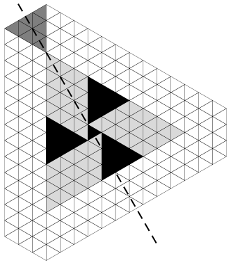
Figure 6: Two hexagonal regions with holes, corresponding to Families A and B; on the left with parameters $s=4$, $t=0$, $n=4$, $\mu=5$, on the right with parameters $s=3$, $t=0$, $n=6$, $\mu=3$.

Theorem 19 (Family B).

Let $\mu$ be an indeterminate, and let $r$ and $n$ be positive integers. If $n$ is an odd number, then

$$D_{2r-1,0}(n)=\prod_{i=r}^{(n-1)/2}\!R_{2r-1,0}(i),$$

where

$$R_{2r-1,0}(n)=-\frac{\bigl{(}\mu+2n+4r-4\bigr{)}_{\!n-r+1}\,\bigl{(}\mu+2n+4r-3\bigr{)}_{\!n-r}\left(\frac{\mu}{2}+2n+r-\frac{1}{2}\right)^{\!2}_{\!n-r}}{\bigl{(}n-r+1\bigr{)}_{\!n-r+1}\,\bigl{(}n-r+1\bigr{)}_{\!n-r}\left(\frac{\mu}{2}+n+2r-\frac{3}{2}\right)^{\!2}_{\!n-r}}.$$

Hence, for $n\geqslant r$ we have $R_{2r-1,0}(n)=D_{2r-1,0}(2n+1)/D_{2r-1,0}(2n-1)$. If $n\geqslant 2r$ is an even number, then $D_{2r-1,0}(n)=0$.

Proof.

According to Proposition 14 we have $D_{2r-1,0}(n)=1$ if $n<2r$. When $n$ is odd this is compatible with the asserted formula, since in this case the product is empty.

The tiling regions corresponding to Family B look like the ones for Family A (with the difference that the three outer holes have odd sizes). We first give a combinatorial argument for the case when $n\geqslant 2r$ is even, i.e. the case where the determinant vanishes. An example for this situation is displayed on the right part of Figure 6: By declaring the light-gray lozenges to be holes, we get a hexagonal region with a single triangular hole, as described before. The difference now is that $D_{2r-1,0}(n)$ performs a weighted count. This is the reason for the value $0$ for even $n$, since there are as many tilings with weight $+1$ as there are with weight $-1$. This can be seen as follows.

In Figure 6 (right picture) we identify the border of the original lozenge-shaped region: its left vertical side starts at the top-most vertex of the smallest black triangle. The lower $2r-1$ unit segments of this side lie inside the black region, while each of the upper $n-2r+1$ unit segments may or may not be covered by a rhombus when the whole region is tiled. For a particular (cyclically symmetric) rhombus tiling, the number of unit segments which are not crossed by a horizontal rhombus corresponds to the cardinality of the set $I$ in (2.1), and hence its parity determines whether this tiling is counted with weight $+1$ or with weight $-1$ (note that $s-t=2r-1$ is odd).

We now look at the lozenge-shaped region between the upper part of the above-mentioned vertical line and the dark-gray shaded triangle (see the right part of Figure 6); the tilings of this lozenge correspond to a rectangle in which $|I|$ lattice paths connect two opposite sides. Hence there are also $|I|$ horizontal rhombi crossing the vertical side of the dark-gray triangle. Inside the dark-gray triangle a rhombus tiling corresponds to paths that start at the $|I|$ horizontal rhombi; this situation is depicted in Figure 7 where the start positions are shown as black rhombi. Each path must end somewhere on the lower side of the triangle and its last rhombus will share an edge with the boundary of the triangle. All other segments of the lower side are crossed by rhombi (also colored black in Figure 7). We see that any tiling with $|I|$ rhombi crossing the vertical side of the triangle forces $n-2r+1-|I|$ rhombi to cross its other side.

By considering the reflection across the dashed line in Figure 6, one recognizes that there are as many cyclically symmetric tilings with $|I|$ rhombi crossing the vertical side of the dark-gray triangle as there are with $n-2r+1-|I|$ such rhombi. Hence, if $n-2r+1$ is an odd number, the weighted count yields $0$. Note that this argument establishes an alternative proof of Lemma 3.

However, to prove the full statement of the theorem, we take a different approach (which also covers the already discussed cases). Similar to the proof of Theorem 18, one can reduce $D_{2r-1,0}$ to $D_{1,0}$. $D_{2r-1,0}(n)$ corresponds to a triangular hole of size $\mu+6r-5$ whose distance to the boundary of the hexagon is $n-2r+1$, while for $D_{1,0}(n)$ we have a hole of size $\mu+1$ and distance $n-1$. Hence

$$D_{2r-1,0}(n)=D_{1,0}(n-2r+2)\big{|}_{\mu\to\mu+6r-6}.$$

The proof is completed by noting that the above expression for $R_{2r-1,0}(n)$ follows immediately from the one for $R_{1,0}(n)$ in Proposition 9 by replacing $n$ by $n-r+1$ and $\mu$ by $\mu+6r-6$. ∎

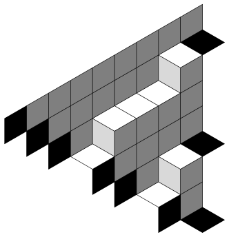
Figure 7: A tiled triangular region of size $9$ with $|I|=3$ “paths” entering from the right, of lengths $7$, $3$, and $0$, respectively; consequently, $9-3=6$ rhombi have to cross the lower left boundary of the region.

The tiling regions for Families C and D are more complicated, and in particular we cannot simplify the different holes and borders to a single large triangular hole. For this reason, the proof strategy applied to Families A and B does not work. So far we have not been able to come up with a proof and therefore we state the following two formulas as conjectures.

Conjecture 20 (Family C).

Let $\mu$ be an indeterminate and let $n$ and $r$ be positive integers. If $n\geqslant r$ then

$$D_{2r,1}(2n)=\frac{(\mu-1)\,\bigl{(}\mu+2r\bigr{)}_{\!2r-1}}{(2r)!}\cdot\prod_{i=r}^{n-1}R_{2r,1}(i),$$

where

$$R_{2r,1}(n)=-\frac{(2n+2r)(\mu+2n+2r-1)(\mu+2n+2r)\,\bigl{(}\mu+2n+4r\bigr{)}^{\!2}_{\!n-r}\left(\frac{\mu}{2}+2n+r+\frac{3}{2}\right)^{\!2}_{\!n-r+1}}{(2n+1)(2n+2)(\mu+2n+1)\bigl{(}n-r+1\bigr{)}^{\!2}_{\!n-r+1}\left(\frac{\mu}{2}+n+2r+\frac{1}{2}\right)^{\!2}_{\!n-r}}.$$

Hence we have that $R_{2r,1}(n)=D_{2r,1}(2n+2)/D_{2r,1}(2n)$.

Note that for $n<r$ we have $D_{2r,1}(2n)=\bigl{(}\mu+2r-1\bigr{)}_{\!2n}/(2n)!$, according to Proposition 14. The conjectured closed form for $D_{1,2r}(n)$ can be obtained via Theorem 17.

Conjecture 21 (Family D).

Let $\mu$ be an indeterminate and let $n\geqslant 1$ and $r\geqslant 0$ be integers. Then

$$D_{-1,2r}(2n)=\prod_{i=0}^{n-1}R_{-1,2r}(i),$$

where

$$R_{-1,2r}(n)=\begin{cases}\displaystyle-\frac{\bigl{(}\mu+2n-1\bigr{)}_{\!2r}\,\bigl{(}\mu+2n-3\bigr{)}_{\!2r+1}\,\bigl{(}\mu+2n+4r\bigr{)}^{\!2}_{\!n-r}\left(\frac{\mu}{2}+2n+r+\frac{1}{2}\right)^{\!2}_{\!n-r-1}}{\bigl{(}2n+1\bigr{)}_{\!2r}\,\bigl{(}2n+2\bigr{)}_{\!2r+1}\,\bigl{(}n-r\bigr{)}^{\!2}_{\!n-r}\left(\frac{\mu}{2}+n+2r+\frac{1}{2}\right)^{\!2}_{\!n-r-1}},&\text{if }n>r,\\ \rule{0.0pt}{24.0pt}\displaystyle\frac{(3-\mu)\,\bigl{(}\mu+2r-2\bigr{)}_{\!2r}\,\bigl{(}\mu+2r-1\bigr{)}_{\!2r}}{\bigl{(}2r+1\bigr{)}_{\!2r}\,\bigl{(}2r+1\bigr{)}_{\!2r+1}},&\text{if }n=r,\\ \rule{0.0pt}{24.0pt}\displaystyle\frac{\bigl{(}\mu+2n-2\bigr{)}_{\!2r}\,\bigl{(}\mu+2n-1\bigr{)}_{\!2r}}{\bigl{(}2n+1\bigr{)}_{\!2r}\,\bigl{(}2n+2\bigr{)}_{\!2r}},&\text{if }n<r.\end{cases}$$

Hence, we have that $R_{-1,2r}(n)=D_{-1,2r}(2n+2)/D_{-1,2r}(2n)$.

Corollary 22 (Family E).

Let $\mu$ be an indeterminate and let $n\geqslant r\geqslant 1$ be integers. Then:

$$\frac{D_{2r-1,1}(2n)}{D_{2r-1,1}(2n-1)} =\frac{\bigl{(}\mu+2n+4r-4\bigr{)}_{\!n-r+1}\left(\frac{\mu}{2}+2n+r-\frac{1}{2}\right)_{\!n-r}}{\bigl{(}n-r+1\bigr{)}_{\!n-r+1}\left(\frac{\mu}{2}+n+2r-\frac{3}{2}\right)_{\!n-r}},$$

$$\frac{D_{1,2r-1}(2n)}{D_{1,2r-1}(2n-1)} =\frac{\bigl{(}\mu+2n-1\bigr{)}_{\!2r-2}\,\bigl{(}\mu+2n+4r-4\bigr{)}_{\!n-r+1}\left(\frac{\mu}{2}+2n+r-\frac{1}{2}\right)_{\!n-r}}{\bigl{(}2n+1\bigr{)}_{\!2r-2}\,\bigl{(}n-r+1\bigr{)}_{\!n-r+1}\left(\frac{\mu}{2}+n+2r-\frac{3}{2}\right)_{\!n-r}}.$$

Proof.

Using Theorems 18 and 19, we can express the above quotients in terms of known determinants, by using the Desnanot-Jacobi-Dodgson identity (DJD):

$$D_{2r-2,0}(2n+1)D_{2r-1,1}(2n-1)=D_{2r-2,0}(2n)D_{2r-1,1}(2n)-\cancelto{0}{D_{2r-1,0}(2n)}D_{2r-2,1}(2n),$$

where $D_{2r-1,0}(2n)=0$ only if $n\geqslant r$. Therefore

$$\frac{D_{2r-1,1}(2n)}{D_{2r-1,1}(2n-1)}=\frac{D_{2r-2,0}(2n+1)}{D_{2r-2,0}(2n)}\qquad(n\geqslant r).$$

The following fact can be derived similarly:

$$\frac{D_{1,2r-1}(2n)}{D_{1,2r-1}(2n-1)}=\frac{D_{0,2r-2}(2n+1)}{D_{0,2r-2}(2n)}\qquad(n\geqslant r).$$

∎

Corollary 23 (Family F).

Let $\mu$ be an indeterminate and let $n\geqslant r\geqslant 1$ be integers. Then:

$$\frac{D_{-1,2r-1}(2n+1)}{D_{-1,2r-1}(2n)}=\frac{2\,\bigl{(}\mu+2n-2\bigr{)}_{\!2r}\,\bigl{(}\mu+2n+4r-2\bigr{)}_{\!n-r-1}\left(\frac{\mu}{2}+2n+r-\frac{1}{2}\right)_{\!n-r}}{\bigl{(}2n\bigr{)}_{\!2r}\,\bigl{(}n-r+1\bigr{)}_{\!n-r}\left(\frac{\mu}{2}+n+2r-\frac{1}{2}\right)_{\!n-r-1}}.$$

Proof.

Using Theorems 18 and 19, we can express the quotient in terms of known determinants, by using (DJD):

$$D_{-1,2r-1}(2n+1)D_{0,2r}(2n-1)=D_{-1,2r-1}(2n)D_{0,2r}(2n)-\cancelto{0}{D_{0,2r-1}(2n)}D_{-1,2r}(2n),$$

where $D_{0,2r-1}(2n)=0$ only if $n\geqslant r$. Therefore

$$\frac{D_{-1,2r-1}(2n+1)}{D_{-1,2r-1}(2n)}=\frac{D_{0,2r}(2n)}{D_{0,2r}(2n-1)}\qquad(n\geqslant r).$$

∎

Conjecture 24.

There is a combinatorial reciprocity between determinants $D_{s,t}(n)$ which just count cyclically symmetric rhombus tilings (the case when $s-t$ is even) and determinants $D_{s,t}(n)$ which perform a weighted count (the case when $s-t$ is odd). For example, we conjecture that

$$D_{2r-1,0}(2n+1)=D_{0,0}(2n-2r+2)\big{|}_{\mu\to 1-\mu-6n}$$

for $n\geqslant r\geqslant 1$. Note that, when setting $r,n,\mu$ to concrete integers, at least one of the two determinants does not allow the combinatorial interpretation given in Section 2, for instance, because the hole is larger than the hexagon.

We would like to point out that special instances (setting the parameter $r$ to a concrete integer) of the results presented in this last section, in particular Conjectures 20 and 21, may be provable in the same manner as the results in Section 3. However, we don’t see how to use this computer algebra approach to prove them for symbolic $r$, since the extra parameter appears also in the Kronecker delta.

These conjectures are along the same line as Conjecture 37 in [12, page 50], which, for the same reason, we have not been able to prove in [9]. In this related family of determinants, the Kronecker delta is multiplied by $-1$. Obviously, they count the same kind of objects, but total count vs. weighted count change their roles. It would be worthwhile to investigate the connections between these determinants and our determinant $D_{s,t}(n)$, in the spirit of Conjecture 24. First experiments suggest that also the determinants $\tilde{D}_{s,t}(n)$ with negative Kronecker delta comprise several infinite families that have nice evaluations or quotients. The analysis of those should not be too different from what we did in the present paper. Another interesting direction of research would be to find $q$-analogs of all these determinants.

Acknowledgment.

We are grateful to Christian Krattenthaler for helpful comments on an earlier draft of this paper, and for explaining some of the combinatorial background to us, and to Elaine Wong for proofreading and useful suggestions. We thank the anonymous referees for their reports that helped us improve the paper significantly.

References

[1]
Tewodros Amdeberhan and Doron Zeilberger.
Determinants through the looking glass.
Advances in Applied Mathematics, 27(2-3):225–230, 2001.
[2]
George E. Andrews.
Plane partitions (III): The weak Macdonald conjecture.
Inventiones mathematicae, 53(3):193–225, 1979.
[3]
George E. Andrews.
Macdonald’s conjecture and descending plane partitions.
In T. V. Narayana, R. M. Mathsen, and J. G. Williams, editors, Combinatorics, Representation Theory and Statistical Methods in Groups,
volume 57 of Lecture notes in pure and applied mathematics, pages
91–106. Proceedings of the Alfred Young Day Conference, 1980.
[4]
David M. Bressoud.
Proofs and Confirmations: The Story of the Alternating-Sign
Matrix Conjecture.
Cambridge University Press, 1999.
[5]
Mihai Ciucu, Theresia Eisenkölbl, Christian Krattenthaler, and Douglas Zare.
Enumeration of lozenge tilings of hexagons with a central triangular
hole.
Journal of Combinatorial Theory, Series A, 95(2):251–334,
2001.
[6]
Ira Gessel and Gérard Viennot.
Binomial determinants, paths, and hook length formulae.
Advances in Mathematics, 58(3):300–321, 1985.
[7]
Christoph Koutschan.
HolonomicFunctions (user’s guide).
Technical Report 10-01, RISC Report Series, Johannes Kepler
University, Linz, Austria, 2010.
http://www.risc.jku.at/research/combinat/software/HolonomicFunctions/.
[8]
Christoph Koutschan, Manuel Kauers, and Doron Zeilberger.
Proof of George Andrews’s and David Robbins’s -TSPP
conjecture.
Proceedings of the National Academy of Sciences,
108(6):2196–2199, 2011.
[9]
Christoph Koutschan and Thotsaporn Thanatipanonda.
Advanced computer algebra for determinants.
Annals of Combinatorics, 17(3):509–523, 2013.
[10]
Christoph Koutschan and Thotsaporn Thanatipanonda.
Electronic material accompanying the article “A curious family of
binomial determinants that count rhombus tilings of a holey hexagon”, 2017.
Available at http://www.koutschan.de/data/det2/.
[11]
Christian Krattenthaler.
Advanced determinant calculus.
Séminaire Lotharingien de Combinatoire, 42:1–67, 1999.
Article B42q.
[12]
Christian Krattenthaler.
Advanced determinant calculus: A complement.
Linear Algebra and its Applications, 411:68–166, 2005.
[13]
Christian Krattenthaler.
Descending plane partitions and rhombus tilings of a hexagon with
triangular hole.
European Journal of Combinatorics, 27:1138–1146, 2006.
[14]
Bernt Lindström.
On the vector representations of induced matroids.
Bulletin of the London Mathematical Society, 5(1):85–90, 1973.
[15]
Doron Zeilberger.
The holonomic ansatz II. Automatic discovery(!) and proof(!!) of
holonomic determinant evaluations.
Annals of Combinatorics, 11(2):241–247, 2007.