Variance-based Robust Optimization of a Permanent Magnet Synchronous Machine

Abstract

This paper focuses on the application of the variance-based global sensitivity analysis for a topology derivative method in order to solve a stochastic nonlinear time-dependent magnetoquasistatic interface problem. To illustrate the approach a permanent magnet synchronous machine has been considered. Our key objective is to provide a robust design of the rotor poles and of the tooth base in a stator for the reduction of the torque ripple and electromagnetic losses, while taking material uncertainties into account. Input variations of material parameters are modeled using the polynomial chaos expansion technique, which is incorporated into the stochastic collocation method in order to provide a response surface model. Additionally, we can benefit from the variance-based sensitivity analysis. This allows us to reduce the dimensionality of the stochastic optimization problems, described by the random-dependent cost functional. Finally, to validate our approach, we provide the two-dimensional simulations and analysis, which confirm the usefulness of the proposed method and yield a novel topology of a permanent magnet synchronous machine.

I Introduction

Due to the several attractive features, such as high efficiency and power factor, high torque to weight ratio and brushless construction, PM synchronous machines have found recently a wide range of applications in the automotive industry, e.g., [3]. However, in spite of their unquestionable advantages, including also the field weakening capability of 1:5, the Electrically Controlled Permanent Magnet Excited Synchronous Machine (ECPSM) [4], served here as a case study, suffers inherently from the considerable level of the torque pulsation [5]. This, in turn, may result in the mechanical vibration and acoustic noise and, as a consequence, affect the machine performance. From this perspective, the mitigation of the torque fluctuations is a key issue for the design of a permanent magnet (PM) machine.

Yet, in many engineering applications, physical models are very often affected by a relatively large amount of uncertainty [2] , which is caused mainly by the imperfections in manufacturing processes. For example, as a result of the punching and quenching in the assembly of the electric machine, some magnetic properties of the core material can deteriorate [6]. Thus, the solution to the optimization problem may be strongly affected by the uncertainties in both the geometrical and material parameters [1], [7]. In the literature, various methods for suppressing the torque ripple (TR) have been proposed. In general, they are divided into two main groups of the deterministic and stochastic optimization methods. Within this context, the topology optimization in particular seems to be a very powerful methodology, e.g., [8, 9, 5]. Other approaches, which aim to reduce the performance variability, are based on the the statistically originated Taguchi method [10, 11]. Different efficient solutions involve, for example, the use of a gradient indexed method or a perturbation method in order to deal with the ’deterministic’ variations of some model parameters [12].

From this perspective, there is a need to include uncertainty quantification (UQ) in the modeling phase to obtain reliable numerical simulations. For this reason, in our paper we explore the stochastic collocation method (SCM) combined with the polynomial chaos expansion (PCE) [13]. This allows for constructing a suitable surrogate - the so-called response surface model - which can be further incorporated into the topology optimization flow [14, 16]. Our new contribution, in comparison with [16], is first to attain the low RT TR design of the ECPSM under uncertainties in the transient analysis. Secondly, the methodology for solving a stochastic time-dependent magnetoquasistatic interface problem is based on the variance-based sensitivity analysis. The low torque ripple TR design with decreased energy consumption profile, found in this way, allows for improving the PM machine quality by minimizing variations of the output performance functions.

II Stochastic Forward Problem

Specifically, for the optimization, when using gradient methods, it is required to consider an efficient computational model. In this respect, the 3D forward problem has been simplified into the 2D FE model, which still yields accurate computational results, [13] and [16]. Thus, a 2D model can be described using the magnetic vector potential $A$ for the stochastic quasi-linear system of PDEs, defined on $t\in(0,T]$ with $T>0$ and ${{\bf x}}\,=\,(x,y)^{\top}\in\mathrm{D}\subset\mathbb{R}^{2}$ as

$$\left\{\begin{array}[]{l l}\nabla\cdot\left(\upsilon_{\scalebox{0.55}{{\rm Fe\,}}}\left({\bf x},|\nabla A(\theta)|^{2},\xi_{1}\right)\nabla A(\theta)\right)+\sigma(\xi_{4})\partial_{t}A(\theta)=J_{i}({\bf x},t),&\\ \nabla\cdot\left(\upsilon_{\scalebox{0.55}{{\rm air\,}}}\left({\bf x},\xi_{2}\right)\nabla A(\theta)\right)=0,&\\ \nabla\cdot\left(\upsilon_{\scalebox{0.55}{{\rm PM\,}}}({\bf x},{{\xi_{3}}})\nabla A(\theta)\right)=\nabla\cdot\upsilon_{\scalebox{0.55}{{\rm PM\,}}}({{\bf x},{\xi_{3}}}){\rm{\bf M}}(\bf x),\quad\quad\quad\quad~{}~{}\mathrm{(1)}\\ \end{array}\right.$$

endowed with both boundary and initial conditions, where $\theta:=({\bf x},t;{\bm{\xi}})\in D\times(0,T]\times\Omega$ with the domain $\rm{D}$, which refers to the sextant region; $\sigma(\xi_{4})=\sigma_{\scalebox{0.55}{{\rm Fe\,}}}(1+\delta_{4}\xi_{4})$ represents conductivity. $J_{i}({\bf x},t)$, $i=1,2,3$ denotes an excitation current density and $\Omega$ is a sample space; ${\bf M}$ represents the remanent flux density of the PM, while ${\bm{\upsilon}}$ denotes the reluctivity. In particular, a stochastic model for $\upsilon(\cdot;\bm{\xi})$ is given by

$${\upsilon}(\theta)=\left\{\begin{array}[]{ll}\upsilon_{\scalebox{0.55}{{\rm Fe\,}}}({\bf x},|\nabla A(\theta)|^{2})(1+\delta_{1}\xi_{1})&\textrm{for}\;\;{\bf x}\in{\rm D}_{\scalebox{0.55}{{\rm Fe\,}}}\\ \upsilon_{\scalebox{0.55}{{\rm air\,}}}({\bf x})\,(1+\delta_{2}\xi_{2})&\textrm{for}\;\;{\bf x}\in{\rm D}_{\scalebox{0.55}{{\rm air\,}}}\\ \upsilon_{\scalebox{0.55}{{\rm PM\,}}}({\bf x})\,(1+\delta_{3}\xi_{3})&\textrm{for}\;\;{\bf x}\in{\rm D}_{\scalebox{0.55}{{\rm PM\,}}},\\ \end{array}\right.$$ (2)

where ${\bm{\xi}}=(\xi_{1},\xi_{2},\xi_{3},\xi_{4})$ are assumed to be random variables, defined on some probability space $(\mathrm{\Omega},\mathcal{F},\mathbb{P})$ with the event space $\mathrm{\Omega}$, sigma-algebra $\mathcal{F}$ and probability measure $\mathbb{P}$. For the scalings $\delta_{j}$, see below.

III Uncertainty Quantification $\&$ Sobol Decomposition

For the uncertainty quantification, we consider ${\bf p}({\bm{\xi}})$ = [$\upsilon_{\scalebox{0.55}{{\rm Fe\,}}}(\xi_{1})$, $\upsilon_{\scalebox{0.55}{{\rm air-gap\,}}}(\xi_{2})$, $\upsilon_{\scalebox{0.55}{{\rm PM\,}}}(\xi_{3})$, $\sigma(\xi_{4})$] $\in\Pi$, where ${\xi_{j}},j=1,\ldots,4$ are independent and identically uniformly distributed in the interval $[-1,1]^{4}$ with the constant magnitude $\delta_{j}=0.1$, for $j=1,2,3$ and $\delta_{4}=0.05$. Thus, we assume a joint probability density function $g:\Pi\rightarrow\mathbb{R}$, which is associated with $\mathbb{P}$, and that function $u$ is a square integrable function. with $\mathbb{P}$, that defines an inner-product $<.,.>_{g}$ and a space of $L^{2}_{g}$ quadratically integrable functions $u$ that can be approximated by

$$u\left({{\bf x},t;{\bf p}}\right)\doteq\sum\limits_{i=0}^{N}{{{\alpha}}_{i}\left({\bf x},t\right)}{{{\Psi}_{i}}}\left({{\bf p}}\right)$$ (3)

with a priori unknown coefficient functions ${{\alpha}}_{i}$ and predetermined basis polynomials ${{\Psi}_{i}}$ with the orthogonality property $\mathbb{E}\left[{\Psi}_{i}{\Psi}_{j}\right]=\delta_{ij}$. Here, $\mathbb{E}$ is the expected value, associated with $\mathbb{P}$. For the calculation of ${\alpha}_{i}$, we applied the SCM with the Stroud-3 formula [16], which yields the solution at each quadrature node ${{\bm{\xi}}}^{(k)}$, $k=1,\ldots,K$ of the problem  (1). Next, the multi-dimensional quadrature rule with associated weights $w_{k}$ is used for projecting function $u_{k}$ into the basis ${{\Psi}_{i}}$ as

$${\alpha}_{i}({\bf x},t)\doteq\sum\limits_{k=1}^{K}u\left({\bf x},{t,\,{\bf p}^{(k)}}\right)\Psi_{i}\left({{\bf p}}^{(k)}\right){w_{k}},$$ (4)

Finally, the statistical moments are approximated by

$$\mathbb{E}\left[{{{u}}\left({\bf x},{t;{{\bf p}}}\right)}\right]\;\doteq\;{{\alpha}}_{0}({\bf x},t),\mbox{Var}\left[{{{u}}\left({\bf x},{t;{{\bf p}}}\right)}\right]\;\doteq\sum\limits_{i=1}^{N}{\left|{{{\alpha}}_{i}(t)}\right|^{2}},$$ (5)

assuming $\Psi_{0}=1$ [13]. Additionally, in order to assess the impact of each uncertain parameter on the output variation, the variance-based sensitivity analysis has been applied. It is based on the Sobol indices, which allow for decomposing the total variance in the form [17]

$$S:=\sum_{k=1}^{K}S_{i}+\sum_{1\,\leq i,<j,\leq K}S_{ij}+\ldots+S_{1,2,\ldots,K}.$$ (6)

Here, $S=\mbox{Var}\left[{{{u}}\left({\bf x},{t;{{\bf p}}}\right)}\right]$ and $S_{i_{1}\cdots,i_{S}}$ denote the total and partial variances, while the PC-based Sobol indices are defined using (3) as [18]

$$SU_{i_{1},\dots,i_{S}}:=S_{i_{1},\cdots,i_{S}}/S,$$ (7)

where

$$S\doteq\sum_{|k|=1}^{K}v_{k}^{2},\quad S_{i_{1}\cdots,i_{S}}\doteq\sum_{|k|\leq K,k\in L}v_{k}^{2}$$ (8)

with $L:=\{k|k_{i}\geq 1,i\in\{i_{1},\dots,i_{S}\};k_{j}=0,j\notin\{i_{1},\dots,i_{S}\}\}$. Moreover, the total sensitivity indices can be easily computed, when mixed terms are involved in the summation, see for example [18].

IV Stochastic Optimization Problem

For the optimization it is necessary to define some criteria, which allow to asses the design of a PM machine. On the one hand, our objective is to suppress the ripple torque TR. Therefore, as the first objective we consider the electromagnetic torque (ET) $T$, which in practical applications can be calculated using the virtual work method for a specific position as a partial derivative of the magnetic co-energy $W_{\rm M}$ w.r.t. the angular displacement as $\vartheta$ [3]

$$T\left(\theta\right):=\frac{\partial W_{\mathrm{M}}}{\partial{\vartheta}}.$$ (9)

It should be noted that the electromagnetic torque fluctuations are proportional to the partial derivative of the co-energy stored in a system versus time $\partial_{t}W_{\rm M}$. On the other hand, our second objective is to minimize electromagnetic losses, defined as

$$P_{\mathrm{avg}}(\theta):=\int_{D}Q\left(\theta\right)\mathrm{d}{\bf x}+\frac{1}{2}\int_{D}\partial_{t}W_{M}\left(\theta\right)\,\mathrm{d}{\bf x},$$ (10)

where the first term of the above equation refers to the Joule loss, while the second one - in the case of the time periodic excitation - can be interpreted as the energy dissipation due to the irreversible material behaviour (hysteresis). Therefore, we formulate the time-dependent stochastic magnetoquasistatic interface problem for the cost functional, which allows for considering both objectives, by incorporating (9) into (10)

$$F\left(\bm{\xi}\right):=\frac{1}{2}\left[\int_{0}^{T}\,\left|{P_{\rm r}(\partial_{t}A({\bf x},\bm{\xi})})\right|^{2}\,+\left|{P_{\rm h}(\partial_{t}\nabla A({\bf x},\bm{\xi})})\right|^{2}\right]\>\mbox{d}t,$$ (11)

with the first term $P_{\rm r}(\partial_{t}A({\bf x},\bm{\xi})):=\int_{D}\sigma{\partial_{t}A}\cdot{\partial_{t}A}\,\mathrm{d}{\bf x}$ and ${P_{\rm h}(\partial_{t}\nabla A({\bf x},\bm{\xi})}):=\int_{D}\partial_{t}\upsilon{\nabla A}\cdot{\nabla A}\,\mathrm{d}{\bf x}$. Here, we just multiply the hysteresis losses by a factor of two, instead of using the average weighted method. Finally, our stochastic optimization problem with the discreet weak form of eq. (1) as the stochastic constraint has been defined as

$$\begin{array}[]{lll}\min\limits_{\bf p}&:&{\mathbb{E}}\left[{F({\bf p})}\right]\\ \mathrm{s.t.}&:&{\rm{\bf K}}\left({\bf p}^{k}\right){\rm{\bf A}}^{k}={\rm{\bf f}}^{k},\;k=1,...,K,\\[2.15277pt] &&g_{1}({\bf x})=|{\rm D}_{\rm{{\scalebox{0.55}{FEr}}}}|/|{\rm D}_{\rm{{\scalebox{0.55}{FEr0}}}}|-S_{\rm{{\scalebox{0.55}{FEr}}}}=0,\\[1.07639pt] &&g_{2}({\bf x})=|{\rm D}_{\rm{{\scalebox{0.55}{PM}}}}|/|{\rm D}_{\rm{{\scalebox{0.55}{PM0\,}}}}|-S_{\rm{{\scalebox{0.55}{PM\,}}}}=0,\\[1.07639pt] &&g_{3}({\bf x})=|{\rm D}_{\rm{{\scalebox{0.55}{FEs}}}}|/|{\rm D}_{\rm{{\scalebox{0.55}{FEs0}}}}|-S_{\rm{{\scalebox{0.55}{FEs}}}}=0,\\[1.07639pt] \end{array}$$ (12)

where $g_{1}({\bf x})$, $g_{2}({\bf x})$ and $g_{3}({\bf x})$ are the deterministic area constraints ${\color[rgb]{0,0,0}|D|}$ related to the initial areas of iron $\left({\rm D}_{\rm FEr0}\right)$ and PM, $\left({\rm D}_{\rm PM0}\right)$ rotor poles and the tooth base in the stator $\left({\rm D}_{\rm FEs0}\right)$, with some prescribed coefficients, such as $S_{\rm{FEr}}$, $S_{\rm{PM}}$ and $S_{\rm{FEs}}$, respectively. The stiffness and mass matrix is denoted by ${\bf K}$. Furthermore, in order to solve the above-mentioned optimization problem, we can benefit from the Sobol decomposition and use the partial derivative of the variances (7) or the partial derivative of the variances with terms of the mixed indices included. In this way, it is also possible to reduce the dimensionality of the optimization problem by eliminating these variables, which results in a small range of the variance-based sensitivity those variables that contribute lowest to the variance-based sensitivity.

TABLE I: Main Parameters of the ECPSM Design [5].

Parameter [unit]	Symbol	Value
Pole number	2p	12
Stator outer radius [mm]	$r_{\rm ostat}$	67.50
Stator inner radius [mm]	$r_{\rm istat}$	41.25
One part stator axial length [mm]	$l_{\rm as}$	35.0
Slot openning width [mm]	$w_{\rm oslot}$	4.0
Number of slots	$ns$	36
Number of phases	$m$	3
Permanent Magnet pole	${\rm NdFeB}$	12
PM thickness [mm]	$t_{\rm m}$	3.0
Remanent flux density [T]	$B_{\rm r}$	1.2

V Numerical Results & Discussion

We applied the proposed procedure to design both the rotor poles as well as the base tooth in the stator of the ECPSM machine at on-load state. The main parameters of the PM are given in Table I. For the simulation of a 2D FEM model at the on-load condition, the COMSOL 3.5a has been applied with $I_{i}({\bf x},t)=15[A]$, $i=1,2,3$. We implemented the variance-based algorithm for the topology optimization using matlab scripts in MATLAB 7.10. The FEM model consists of a triangular mesh with the second order Lagrange polynomials. The areas of the one-pole pair rotor in the initial 2D model were divided into 360 and 480 voxels for the iron and the PM poles, respectively. In addition, the base tooth in the stator consisted of 512 voxels. As a reference model, we used the model depicted in Fig. 2a with the same area of the PM rotor pole as in the optimized structure, shown on Fig. 1b. Hence, we investigated only the impact of the shape change of the PM rotor poles, including shape changes of iron poles and tooth base in the stator, on the performance functions. To control the geometrical complexity of the various shapes, a version of the level set method – based on the topological derivative as introduced in [19] – can be used together with the regularization term, as in [9], [20], [16]. To solve a stochastic direct problem, represented by (1) the SCM with the PC expansion has been applied, where the input variations have been described by a uniform distribution. Due to the assumed probabilistic density function, the Legendre polynomial of order 2 has polynomials up to order 2 have been used as the basis. Moreover, the application of the Stroud-3 formula for the ECPSM machine with four random parameters leads to $K=8$ grid points in the four-dimensional parameter space. The structure of the electric machine, with the optimized shapes of rotor poles and stator teeth, has been found in the 12th iteration of the optimization process, after approximately 8 hours of computing. Both structures, before and after the optimization, are shown in Figs. 1 and 2, respectively. Subsequently, for reference and optimized topology, the ET is calculated over three cycles. The results for the mean and standard deviations of the ET are depicted in Fig. 3. In order to investigate the influence of the robust optimization on the back EMF, we present the mean and standard deviations calculated of the back EMF in Fig. 4. In addition, the spectral analysis applying FFT to the back EMF, as shown in Fig. 4, has been carried out.

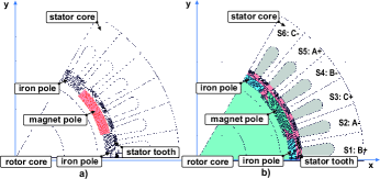
Figure 1: ECPSM topology for (a) initial and (b) optimized configurations.

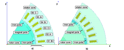
Figure 2: ECPSM topology for (a) reference and (b) optimized configurations.

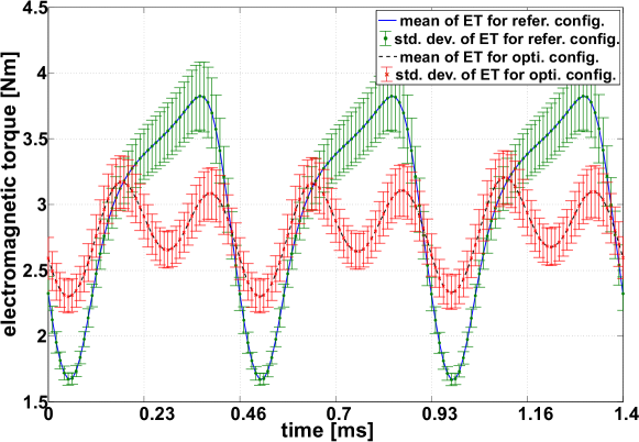
Figure 3: Mean and standard deviation of of the electromagnetic torque (ET) for reference and optimized ECPSM configurations.

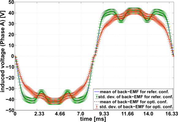
Figure 4: Mean and standard deviation of the back EMF for reference and optimized ECPSM configurations.

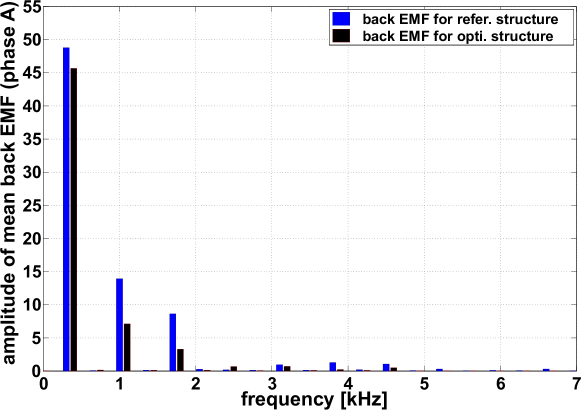
Figure 5: FFT analysis of the back EMF for reference and optimized ECPSM configurations.

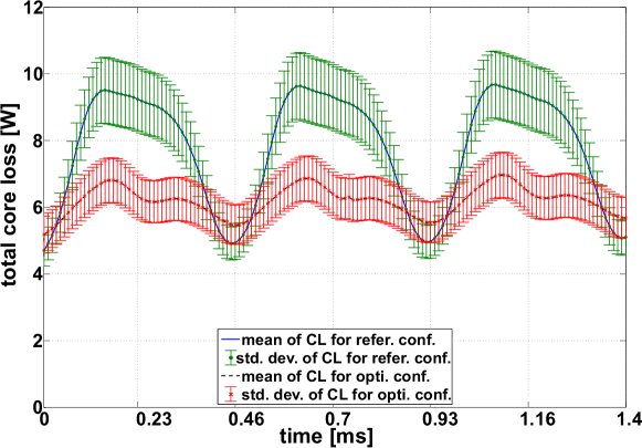
Figure 6: Mean and standard deviation of of the core loss (CL) for reference and optimized ECPSM configurations.

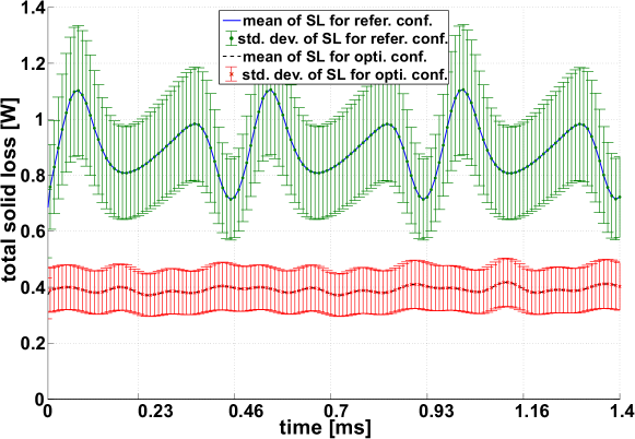
Figure 7: Mean and standard deviation of the solid (resistive) loss (SL) for reference and optimized ECPSM configurations.

TABLE II: Statistics of some Physical Parameters of the ECPSM Reference and Optimized Models at On-load Mode.

	Reference	Optimized	Decrease
Quantity [unit]	topology	topology	/increase
Expectation of the ET [Nm]
Rectified mean value	2.986	2.805	6.05$\%$ $\downarrow$
RMS value	3.067	2.818	8.12$\%$ $\downarrow$
Std. dev. of the ET [Nm]
Rectified mean value	0.166	0.165	0.71$\%$ $\downarrow$
RMS value	0.177	0.166	6.25$\%$ $\downarrow$
Expectation of the FL [Wb]
Rectified mean value	0.014	0.013	5.46$\%$ $\downarrow$
RMS value	0.016	0.015	6.65$\%$ $\downarrow$
Std. dev. of the FL [mWb]
Rectified mean value	0.751	0.750	0.15$\%$ $\downarrow$
RMS value	0.862	0.844	2.13$\%$ $\downarrow$
Expectation of the CL [W]
Rectified mean value	7.812	6.198	20.66$\%$ $\downarrow$
RMS value	7.984	6.212	22.19$\%$ $\downarrow$
Std. dev. of the CL [W]
Rectified mean value	0.808	0.638	21.06$\%$ $\downarrow$
RMS value	0.827	0.638	22.85$\%$ $\downarrow$
Expectation of the SL [W]
Rectified mean value	0.896	0.392	56.27$\%$ $\downarrow$
RMS value	0.902	0.391	56.54$\%$ $\downarrow$
Std. dev. of the SL [W]
Rectified mean value	0.185	0.080	56.51$\%$ $\downarrow$
RMS value	0.186	0.080	56.80$\%$ $\downarrow$
Mean of others quantities
Ripple torque [%]	70.31	32.13	54.30$\%$ $\downarrow$

In practical calculations for the estimation of the electromagnetic losses, the Berttoti model has been applied[21]. The results of this analysis for both configurations have been depicted in Figs. 5 and 6, respectively. Finally, the results for the topology optimization for the quantities such as the electromagnetic torque (ET), the flux linkage (FL), the core loss (CL), and the solid loss (SL) have been summarized in Table II.

VI Conclusion

The variance-based topology optimization has been successfully implemented to achieve a low torque ripple as well as reduce electromagnetic losses using a 2D design of an Electrically Controlled Permanent Magnet Excited Synchronous Machine. Moreover, the same methodology may be extended to a full 3D treatment, however with the inevitable higher computational burden associated with the solution of a 3D stochastic forward problem. The proposed procedure results in suppressing the mean rms value of the ripple torque (RT) by 54$\%$, and in reducing the mean rms value of the core losses (CL) and and the solid losses (SL) by 22$\%$ and 56$\%$, respectively. A drawback of the proposed method is the associated reduction of the rms value of the electromagnetic torque by 8$\%$, and this issue will be addressed in future research.

References

- [1] A. Abou-Elyazied Abdallh, G. Crevecoeur, and L. Dupré, ”A robust inverse approach for magnetic material characterization in electromagnetic devices with minimum influence of the air-gap uncertainty.” IEEE Trans. on Magn. vol. 47 pp. 4364–4367, 2011.
- [2] I. Babučka, F. Nobile, R. Tempone, ”A stochastic collocation method for elliptic partial differential equations with random input data.” SIAM J. Numer. Anal. vol. 52 pp. 317–355. 2010.
- [3] F. Gieras, M. Wing, Permanent magnet motor technology, John Wiley Sons Ltd. 2008.
- [4] H. May, R. Pałka, P. Paplicki, S. Szkolny, and W.R. Canders, “New concept of permanent magnet excited synchronous machines with improved high-speed features,” Arch. of Electr. Engineer., vol. 60, pp. 531–540, 2011.
- [5] P. Putek, P. Paplicki, and R. Pałka, “Low cogging torque design of permanent magnet machine using modified multi-level set method with total variation regularization,” IEEE Trans. on Magn., vol. 50, pp. 657–660, 2014.
- [6] Z. Gmyrek, A. Cavagnino, and L. Ferraris, “Estimation of the magnetic properties of the damaged area resulting from the punching process: experimental research and FEM modeling,“ IEEE Trans. Ind. Appl. vol. 49, pp. 2069–2077, 2013.
- [7] P. Sergeant, G. Crevecoeur, L. Dupre, and A. van den Bossche, ”Characterization and optimization of a permanent magnet synchronous machine,” COMPEL, vol. 28, pp. 272–284, 2008.
- [8] D. H. Kim, J. K, Sykulski, and D. A. Lowther, “The Implications of the Use of Composite Materials in Electromagnetic Device Topology and Shape Optimization,” IEEE Trans. on Magn. vol. 45, pp. 1154–1156, 2009.
- [9] S. H. Lim, S. J. Min, and J. P. Hong, “Low Torque Ripple Rotor Design of the Interior Permanent Magnet Motor Using the Multi-phase Level-Set and Phase-Field Concept,” IEEE Trans. on Magn. vol. 48, pp. 907–909, 2012.
- [10] M. S. Islam, R. Islam, T. Sebastian, A. Chandy, and S. A. Ozsoylu, “Cogging torque minimization in PM motors using robust design approach,” IEEE Trans. on Magn. vol. 47, pp. 1661–1669, 2011.
- [11] J. T. Li, Z. J. Liu, M. A. Jabbar, and X. K. Gao, ”Design optimization for cogging torque minimization using response surface methodology,” IEEE Trans. on Magn. vol. 40, pp. 1176–1180, 2004.
- [12] N. -K. Kim, D. -H. Kim, D. -W. Kim, H. -G. Kim, D. A. Lowther, and J. K. Sykulski, ”Robust optimization utilizing the second-order design sensitivity information,” IEEE Trans. on Magn. vol. 46, pp. 3117–3120, 2010.
- [13] D. Xiu, “Efficient Collocational Approach for Parametric Uncertainty Analysis,” Commun. in Comput. Phys., vol. 2, pp. 293–309, 2007.
- [14] P. Putek, P. Meuris, R. Pulch, E. J. W. ter Maten, W. Schoenmaker, and M. Günther, “Uncertainty quantification for a robust topology optimization of power transistor devices,” IEEE Trans. on Magn., vol. 52, 2016.
- [15] P. Putek, P. Paplicki, and R. Pałka R. “Topology optimization of rotor poles in a permanent-magnet machine using level set method and continuum design sensitivity analysis,” Compel, vol. 33, pp. 711–28, 2014.
- [16] P. Putek, R. Pulch, A. Bartel, E.J.W. ter Maten, M. Günther, and K.M. Gawrylczyk, “Shape and topology optimization of a permanent-magnet machine under uncertainties,” J. Math. Industry, vol. 6, 2016.
- [17] I. M Sobol, “Sensitivity estimates for nonlinear mathematical models,”Math. Modeling Comput. Exp. , vol. 1, pp.407–413, 1993.
- [18] B. Sudret, “Global sensitivity analysis using polynomial chaos expansions,” Rel. Eng. Syst. Safety, vol.93, pp. 964-979, 2008.
- [19] S. Amstutz and H. Andrä, “A new algorithm for topology optimization using a level-set method.” J. Comput. Phys. vol. 216, pp. 573-588, 2006.
- [20] P. Putek, “Mitigation of the cogging torque and loss minimization in a permanent magnet machine using shape and topology optimization.” Engineering_Computations, vol. 33, pp. 831-854. 2016.
- [21] G. Bertotti, “General Properties of Power Losses in Soft Ferromagnetic Materials.” IEEE Trans. on Magn. vol. 24, pp. 621–630, 1988.