Type II supernova spectral diversity I: Observations, sample characterization and spectral line evolution

Abstract

We present 888 visual-wavelength spectra of 122 nearby type II supernovae (SNe II) obtained between 1986 and 2009, and ranging between 3 and 363 days post explosion. In this first paper, we outline our observations and data reduction techniques, together with a characterization based on the spectral diversity of SNe II. A statistical analysis of the spectral matching technique is discussed as an alternative to non-detection constraints for estimating SN explosion epochs. The time evolution of spectral lines is presented and analysed in terms of how this differs for SNe of different photometric, spectral, and environmental properties: velocities, pseudo-equivalent widths, decline rates, magnitudes, time durations, and environment metallicity. Our sample displays a large range in ejecta expansion velocities, from $\sim 9600$ to $\sim 1500$ km s^-1 at 50 days post explosion with a median H_α value of 7300 km s^-1. This is most likely explained through differing explosion energies. Significant diversity is also observed in the absolute strength of spectral lines, characterised through their pseudo-equivalent widths. This implies significant diversity in both temperature evolution (linked to progenitor radius) and progenitor metallicity between different SNe II. Around 60% of our sample show an extra absorption component on the blue side of the H_α P-Cygni profile (“Cachito” feature) between 7 and 120 days since explosion. Studying the nature of Cachito, we conclude that these features at early times (before $\sim 35$ days) are associated with Si II $\lambda 6355$, while past the middle of the plateau phase they are related to high velocity (HV) features of hydrogen lines.

I. Introduction

Supernovae (SNe) exhibiting prevalent Balmer lines in their spectra are known as Type II SNe (SNe II henceforth, Minkowski 1941). They are produced by the explosion of massive ($>8$ M_⊙) stars, which have retained a significant part of their hydrogen envelope at the time of explosion. Red supergiant (RSG) stars have been found at the position of SN II explosion sites in pre-explosion images (e.g. Van Dyk et al., 2003; Smartt et al., 2004, 2009; Maund & Smartt, 2005; Smartt, 2015), suggesting that they are the direct progenitors of the vast majority of SNe II.
Initially SNe II were classified according to the shape of the light curve: SNe with faster ‘linear’ declining light curves were cataloged as SNe IIL, while SNe with a plateau (quasi-constant luminosity for a period of a few months) as SNe IIP (Barbon et al., 1979). Years later, two spectroscopic classes and one photometric were added within the SNe II group: SNe IIn and SNe IIb, and SN 1987A-like, respectively. SNe IIn show long-lasting narrow emission lines in their spectra (Schlegel, 1990), attributed to interaction with circumstellar medium (CSM), while SNe IIb are thought to be transitional objects, between SNe II and SNe Ib (Filippenko et al., 1993). On the other hand, the 1987A-like events, following the prototype of SN 1987A (e.g. Blanco et al., 1987; Menzies et al., 1987; Hamuy et al., 1988; Phillips et al., 1988; Suntzeff et al., 1988), are spectrotroscopically similar to the typical SNe II, however their light curves display a peculiar long rise to maximum ($\sim 100$ days), which is consistent with a compact progenitor. The latter three sub-types (IIn, IIb and 87A-like) are not included in the bulk of the analysis for this paper.
Although it has been shown that SNe II are a continuous single population (e.g. Anderson et al., 2014b; Sanders et al., 2015; Valenti et al., 2016), a large spectral and photometric diversity is observed. Pastorello et al. (2004) and Spiro et al. (2014) studied a sample of low luminosity SNe II. They show that these events present, in addition to low luminosities (M${}_{V}\geq-15.5$ at peak), narrow spectral lines. Later, (Inserra et al., 2013) analyzed a sample of moderately luminous SNe II, finding that these SNe, in contrast to the low luminosity events, are relatively bright at peak (M${}_{V}\leq-16.95$).
In addition to these samples, many individual studies have been published showing spectral line identification, evolution and parameters such as velocities and pseudo-equivalent widths (pEWs) for specific SNe. Examples of very well studied SNe include SN 1979C (e.g. Branch et al., 1981; Immler et al., 2005), SN 1980K (e.g. Buta, 1982; Dwek, 1983; Fesen et al., 1999), SN 1999em (e.g. Baron et al., 2000; Hamuy et al., 2001; Leonard et al., 2002b; Dessart & Hillier, 2006), SN 1999gi (e.g. Leonard et al., 2002a), SN 2004et (e.g. Li et al., 2005; Sahu et al., 2006; Misra et al., 2007; Maguire et al., 2010), SN 2005cs (e.g. Pastorello et al., 2006; Dessart et al., 2008; Pastorello et al., 2009), and SN 2012aw (e.g. Bose et al., 2013; Dall’Ora et al., 2014; Jerkstrand et al., 2014). The first two SNe (1979C and 1980K) are the prototypes of fast declining SNe II (SNe IIL), together with unusually bright light curves and high ejecta velocities. On the other hand, the rest of the objects listed are generally referred to as SNe IIP as they display relatively slowly declining light curves. For faint SNe similar to SN 2005cs, the expansion velocity and luminosity are even lower, probably due to low energy explosions (see Pastorello et al. 2009).
In recent years, the number of studies of individual SNe II has continued to increase, however there are still only a handfull of statistical analyses of large samples (e.g. Patat et al., 1994; Arcavi et al., 2010; Anderson et al., 2014b; Gutiérrez et al., 2014; Faran et al., 2014b, a; Sanders et al., 2015; Pejcha & Prieto, 2015a, b; Valenti et al., 2016; Galbany et al., 2016; Müller et al., 2017). Here we attempt to remedy this situation. The purpose of this paper is to present a statistical characterization of the optical spectra of SNe II, as well as an initial analysis of their spectral features. We have analyzed 888 spectra of 122 SNe II ranging between 3 and 363 days since explosion. We selected 11 features in the photospheric phase with the aim of understanding the overall evolution of visual-wavelength spectroscopy of SNe II with time.
The paper is organized as follows. In section II we describe the data sample. The spectroscopic observations and data reduction techniques are presented in section III. In section IV the estimation of the explosion epoch is presented. In section V we describe the sample properties, while in section VI we identify spectral features. The spectral measurements are presented in section VII while the line evolution analysis and the conclusions are in section VIII and IX, respectively.
In Paper II, we study the correlations between different spectral and photometric parameters, and try to understand these in terms of the diversity of the underlying physics of the explosions and their progenitors.

II. Data sample

Our dataset was obtained between 1986 and 2009 from a variety of different sources. This sample consists of 888 optical spectra of 122 SNe II, of which four were provided by the Cerro Tololo Supernova Survey (CTSS), seven were obtained by the Calán/Tololo survey (CT, Hamuy et al. 1993, PI: Hamuy 1989-1993), five by the Supernova Optical and Infrared Survey (SOIRS, PI: Hamuy, 1999-2000), 31 by the Carnegie Type II Supernova Survey (CATS, PI: Hamuy, 2002-2003) and 75 by the Carnegie Supernova Project (CSP-I, Hamuy et al. 2006, 2004-2009). These follow-up campaigns concentrated on obtaining well-sampled and high-cadence light curves and spectral sequences of nearby SNe, based mainly on 2 criteria: 1) that the SN was brighter than V$\sim 17$ mag at discovery, and 2) that those discovered SNe were classified as being relatively young, i.e., less than one month from explosion.
The redshift distribution of our sample is shown in Figure 1. The figure shows that the majority of the sample have a redshift $\leq 0.03$. SN 2002ig has the highest redshift in the sample with a value of 0.077, while the nearest SN (SN 2008bk) has a redshift of 0.00076. The mean redshift value of the sample is 0.0179 and the median is 0.0152. The redshift information comes from the heliocentric recession velocity of each host galaxy as published in the NASA/IPAC extragalactic Database (NED). These NED values were compared with those obtained through the measurement of narrow emission lines observed within SN spectra and originating from host H II regions. In cases of discrepancy between the two sources, we give priority to our spectral estimations. Two of our objects (SN 2006Y and SN 2007ld) occur in unknown host galaxies. Their redshifts were obtained from the Asiago supernova catalog and from the narrow emission lines within SN spectra originating from the underlying host galaxy, respectively. Table LABEL:t_info lists the sample of SNe II selected for this work, their host galaxy information, and the campaign to which they belong.
From our SNe II sample, SNe IIn, SNe IIb and SN 1987A-like events (SN 2006au and SN 2006V; Taddia et al. 2012) were excluded based on photometric information. Details of the SNe IIn sample can be found in Taddia et al. (2013), while those of the SNe IIb in Stritzinger et al. (2017) and Taddia et al. (2017). The photometry of our sample in the $V-$band was published by Anderson et al. (2014b). More recently, Galbany et al. (2016) released the UBVRIz photometry of our sample obtained by CATS between 1986 and 2003. Around 750 spectra of $\sim 100$ objects are published here for the first time. Now we briefly discuss each of the surveys providing SNe for our analysis.

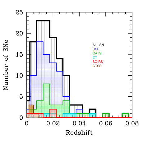
Figure 1.— Distribution of heliocentric redshifts for the 122 SN II in our sample.

II.1. The Cerro Tololo Supernova Survey

A total of 4 SNe II (SN 1986L, SN 1988A, SN 1990E, and SN 1990K) were extensively observed at CTIO by the Cerro Tololo SN program (PIs: Phillips & Suntzeff, 1986-2003). These SNe have been analyzed in previous works (e.g Schmidt et al., 1993; Turatto et al., 1993; Cappellaro et al., 1995; Hamuy, 2001).

II.2. The Calán/Tololo survey (CT)

The Calán/Tololo survey was a program of both discovery and follow-up of SNe. A total of 50 SNe were obtained between 1989 and 1993. The analysis of SNe Ia was published by Hamuy et al. (1996). Spectral and photometric details of six SNe II were presented by Hamuy (2001). In this analysis we include these SNe II and an additional object, SN 1993K.

II.3. The Supernova Optical and Infrared Survey (SOIRS)

The Supernova Optical and Infrared Survey carried out a program to obtain optical and IR photometry and spectroscopy of nearby SNe ($z<0.08$). In the course of 1999-2000, 20 SNe were observed, six of which are SNe II. Details of these SNe were published by Hamuy (2001); Hamuy et al. (2001), Hamuy & Pinto (2002), and Hamuy (2003).

II.4. The Carnegie Type II Supernova Survey (CATS)

Between 2002 and 2003 the Carnegie Type II Supernova Survey observed 34 SNe II. While optical spectroscopy and photometry of these SNe II have been previously used to derive distances (Olivares, 2008; Jones et al., 2009), the spectral observations have not been officially released until now.

II.5. The Carnegie Supernova Project I (CSP-I)

The Carnegie Supernova Project I (CSP-I) was a five year follow-up program to obtain high quality optical and near infrared light curves and optical spectroscopy. The data obtained by the CSP-I between 2004 and 2009 consist of $\sim 250$ SNe of all types, of which 75 correspond to SNe II. The first SN Ia photometry data were published in Contreras et al. (2010), while their analysis was done by Folatelli et al. (2010). A second data release was provided by Stritzinger et al. (2011). A spectroscopy analysis of SNe Ia was published by Folatelli et al. (2013). Recently, Stritzinger et al. (2017) and Taddia et al. (2017) published the photometry data release of stripped-envelope supernovae. The CSP-I spectral data for SNe II are published here for the first time, while the complete optical and near-IR photometry will be published by Contreras et al. (in prep).

III. Observations and data reduction

In this section we summarize our observations and the data reduction techniques. However, a detailed description of the CT methodology is presented in Hamuy et al. (1993), in the case of SOIRS is described in Hamuy et al. (2001) and for CSP-I can be found in Hamuy et al. (2006) and Folatelli et al. (2013).

III.1. Observations

The data presented here were obtained with a large variety of instruments and telescopes, as shown in Table LABEL:t_spec. The majority of the spectra were taken in long-slit spectroscopic mode with the slit placed along the parallactic angle. However, when the SN was located close to the host, it was necessary to pick a different and more convenient angle to avoid contamination from the host. The majority of our spectra cover the range of $\sim 3800$ to $\sim 9500$ Å. The observations were performed with the Cassegrain spectrographs at 1.5-m and 4.0-m telescopes at Cerro Tololo, with the Wide Field CCD Camera (WFCCD) at the 2.5m du Pont Telescope, the Low Dispersion Survey Spectrograph (LDSS2; Allington-Smith et al. 1994) on the Magellan Clay 6.5-m telescope and the Inamori Magellan Areal Camera and Spectrograph (IMACS; Dressler et al. 2011) on the Magellan Baade 6.5-m telescope at Las Campanas Observatory. At La Silla, the observations were carried out with the ESO Multi-Mode Instrument (EMMI; Dekker et al. 1986) in medium resolution spectroscopy mode (at the NTT) and the ESO Faint Object Spectrograph and Camera (EFOSC; Buzzoni et al. 1984) at the NTT and 3.6-m telescopes. We also have 3 spectra for SN 2006ee obtained with the Boller & Chivens CCD spectrograph at the Hiltner 2.4 m Telescope of the MDM Observatory. Table LABEL:t_spec displays a complete journal of the 888 spectral observations, listing for each spectrum the UT and Julian dates, phases, wavelength range, FWHM resolution, exposure time, airmass, and the telescope and instrument used.
The distribution of the number of spectra per object for our sample is shown in Figure 2. Seven SNe (SN 1993A, SN 2005dt, SN 2005dx, SN 2005es, SN 2005gz, SN2005me, SN 2008H) only have one spectrum, while 90% of the sample have between two and twelve spectra. SN 1986L is the object with the most spectra (31), followed by SN 2008bk with 26. On average we have 7 spectra per SN and a median of 6. There are 87 SNe II for which we have five or more spectra, 32 that have ten or more, and 6 objects with over 15 spectra (SN 1986L, SN 1993K, SN 2007oc, SN 2008ag, SN 2008bk and SN 2008if). In the current work, 4% of our obtained spectra are not used for analysis. 3% correspond to spectra with low S/N that does not allow useful extraction of our defined parameters, while 1% are related with peculiarities in the spectra (see Section V for more details). Despite this, these spectra are still included in the data release, and are noted in Table LABEL:t_spec.

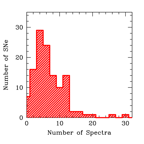
Figure 2.— Histogram of the number of spectra per SN. The distribution peaks at 4 spectra.

III.2. Data reduction

Spectral reduction was achieved in the same manner for all data, using IRAF and employing standard routines, including: bias subtraction, flat-fielding correction, one-dimensional (1D) spectral extraction and sky subtraction, wavelength correction, and flux calibration. Telluric corrections have only been applied to data obtained after October 2004.
In Appendix A (spectral series) we show plots with the spectral series for all SNe of our sample.

IV. Explosion epoch estimations

Before discussing the properties of our sample, in this section we outline our methods for estimating explosion epochs. The non-detection of SNe on pre-discovery images with high cadence is the most accurate method for determining the explosion epoch for any given SN. Explosion epochs based on non-detections are set to the mid-point between SN discovery and non-detection. The representative uncertainty on this epoch is then (MJD${}_{disc}-$MJD${}_{non-det})/2$. However within our sample (and for many other current SN search campaigns) many SNe do not have such accurate constraints from this method due to the low cadence of the observations.
Over the last decade several tools have been published, enabling explosion epoch estimations through matching of observed SN spectra to libraries of spectral templates. Programs such as the Supernova Identification (SNID) code (Blondin & Tonry, 2007), the GEneric cLAssification TOol (Gelato) (Harutyunyan et al., 2008), and superfit (Howell et al., 2005) allow the user to estimate the type of supernova and its epoch by providing an observed spectrum. All perform classifications by comparison using different methods. In our analysis we used only the first two methods: SNID and Gelato. We find that Gelato gives a large percentage of their quality of fit to H_α P-Cygni profile. However, based on our analysis (see Section VIII), the most significant changes with time are observed in the blue part of the spectra (i.e. between 4000 and 6000 Å). Moreover, according to Gutiérrez et al. (2014), the H_α P-Cygni profile shows a wide diversity and there is no clear, consistent evolution with time. In addition, SNID provides the possibility of adding additional templates to improve the accuracy of explosion epoch determinations. We take advantage of this attribute in the following sections by adding new spectral templates, which aid in obtaining more accurate explosion epochs for our sample.
While for many SNe this spectral matching is required to obtain a reliable explosion epoch, a significant fraction of our sample do have explosion epoch constraining SN non-detections before discovery. In cases where the non-detection is $<20$ days before discovery, we use that information to estimate our final values. In cases where this difference is larger than 20 days, we use the spectral matching technique. As a test of our methodology, for non-detection SNe we also estimate explosion epochs using spectral matching to check the latter’s validity (see below for more details).

IV.1. SNID implementation

To constrain the explosion epoch for our sample, we compare the first spectrum of each SN II with a library of spectral templates provided by SNID and then, we choose the best match. For each SN we examined multiple matches putting emphasis on the fit of the blue part of the spectrum between 4000 and 6000 Å. This region contains many spectral lines that display a somewhat consistent evolution with time, unlike the dominant H_α profile at redder wavelengths. Explosion epoch errors from this spectral matching are obtained by taking the standard deviation of several good matches of the observed spectrum of our selected object with those from the SNID library. H_α is the dominant feature in SN II spectra, however its evolution and morphology varies greatly between SNe in a manner that does not aid in the spectral matching technique. We therefore ignore this wavelength region.
The red part of the spectrum can be ignored during spectral matching in a variety of ways. 1) using the SNID options; or 2) checking only the match in the blue part. For the former, SNID gives to the user the alternative to modifying some parameters. In our case, we can constrain the wavelength range using wmin and wmax. Hence, the structure used is: “snid wmin=3500 wmax=6000 spec.dat”. For the latter, we just need to ignore visually the red part of the spectra and explore the matches obtained by SNID until find a good fit in the blue part.
From the SNID library we use those template SNe that have well constrained explosion epochs, meaning SNe II with explosion epoch errors of less than five days (see Table 2). Specifically, we used SN 1999em (Leonard et al., 2002b), SN 1999gi (Leonard et al., 2002a), SN 2004et (Li et al., 2005), SN 2005cs (Pastorello et al., 2006), and SN 2006bp (Dessart et al., 2008). In the database of SNID there are a total of 166 spectra. However, these templates do not provide a good coverage of the overall diversity of SNe II within our sample/the literature. Most of the SNe in the library are relatively ‘normal’, with only one sub-luminous event (SN 2005cs). This means that any non-normal event within our sample will probably have poor constraints on its explosion epoch using these templates. For this reason we decided to use some of our own well-observed SNe II to complement the SNID database.

IV.2. New SNID templates

We created a new set of spectral templates using our own SNe II non-detection limits. SNe II are included as new SNID templates if they have errors on explosion epochs (through non-detection constraints) of less than 5 days. Given this criterion, we included 22 SNe, which show significant spectral and photometric diversity. In this manner, the new SNID templates were constructed using $\sim 150$ spectra and prepared using the logwave program included in the SNID packages. Adding our own template SNe to the SNID database we can now use a total of 27 template SNe II to estimate the explosion epoch. Table 2 shows the explosion epoch and the maximum dates in $V-$band for the reference SNe, as well as the explosion epoch for our new templates. We note an important difference between our templates and previous ones in SNID: for the newer templates epochs are labelled with respect to the explosion epoch, while for the older templates epochs are labelled with respect to maximum light (meaning that one then has to add the “rise time” to obtain the actual explosion date, see Table 2).

IV.3. Explosion epochs for the current sample

With the inclusion of these 22 SNe to SNID we estimated the explosion epoch for our full sample. An example of the best match is shown in Figure 3. We can see that first spectrum of SN 2003iq (October 16th) is best matched with SN 2006bp, SN 2004et, SN 1999em and SN 2004fc 12, 13, 7 and 9 days from explosion, respectively. Taking the average, we conclude that the spectrum was obtained at 10$\pm 7$ days since explosion. Table LABEL:t_info shows the explosion epoch for each SN as well as the method employed to derive it, while Table LABEL:table_explosion shows all the details of spectral matching and non-detection techniques. Appendix B (SNID matches) shows the plots with the best matches for each SN in our sample.

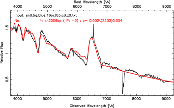
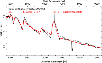
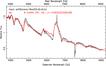
Figure 3.— Best spectral matching of SNe 2003iq using SNID. The plots show SN 2003iq compared with SN 2006bp, SN 2004et, SN 1999em and SN 2004fc at 3, $-3$ and $-3$ and 9 days. As the first three SNe are included in the SNID database, they are respect to the maximum, hence we have to add to them the days between the explosion and the $V-$band maximum (see Table 2) to obtain the explosion epoch. On the other hand, SN 2004fc (included in this work) is respect to the explosion. Therefore, SN 2003iq has a good match with these SNe at 12, 13, 7 and 9 days from explosion, respectively. Taking the average, this means that this spectrum is at 10$\pm 7$ days from explosion.

To check the validity of spectral matching we compare the explosion epoch estimated with this technique and those with non-detections. These two estimations are displayed in Table LABEL:table_explosion. From the second to the seventh column, the spectral matching details are shown (spectrum date, best match found, days from maximum –from the SNID templates– days from explosion, average, and explosion date), while from eighth to tenth, those obtained from the non-detection (non-detection date, discovery date and explosion date). The differences between both methods are presented in the last column. Such an analysis was previously performed by Anderson et al. (2014b) where good agreement was found. With the use of our new templates we are able to improve the agreement between different explosion epoch constraining methods, thus justifying their inclusion. Figure 4 shows a comparison between both methods, where the mean absolute error between them diminishes from 4.2 (Anderson et al., 2014b) to 3.9 days. Also the mean offset decreases from 1.5 days in Anderson et al. (2014b) to 0.5 days in this work. Cases where explosion epochs have changed between Anderson et al. (2014b) and the current work are noted in Table LABEL:t_info. Nevertheless, although this method works well as a substitute for non-detections, exact constraints for any particular object are affected by any peculiarities inherent to the observed (or indeed template) SN. For example, differences in the colour (and therefore temperature) evolution of events can mimic differences in time evolution, while progenitor metallicity differences can delay/hasten the onset of line formation. Further improvements of this technique can only be obtained by the inclusion of additional, well observed SNeII in the future.

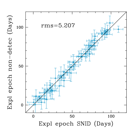
Figure 4.— Comparison between spectral matching and non-detection methods.

V. Sample properties

As mentioned in Section II we have 888 optical spectra of 122 SNe II, however due to low signal-to-noise ($S/N$) we remove 26 spectra of 12 SNe for our analysis. We also remove nine spectra of SN 2005lw because they contain peculiarities that we expect are not intrinsic to the SN (most probably defects resulting from the observing procedure or data reduction). In total, we remove 35 spectra ($\sim 4\%$). Figure 5 shows the epoch distribution of our spectra since explosion to 370 days. One can see the majority (86%) of the spectra were observed between 0 and 100 days since explosion, with a total of 738 spectra. Our earliest spectrum corresponds to SN 2008il at $3\pm 3$ days and SN 2008gr at $3\pm 6$ days from explosion, while the oldest spectrum is at $363\pm 9$ days for SN 1993K. 53% of the spectra were taken prior to 50 days, 3.8% of which were observed before 10 days for 23 SNe. Between $\sim 30$ to 84 days there are 441 spectra of 114 SNe. There are 115 spectra older than 100 days and 27 older than 200 days, corresponding to 45 and 4 SNe, respectively. The average of spectra as a function of epoch from explosion is 60 days, while its median is 46 days.

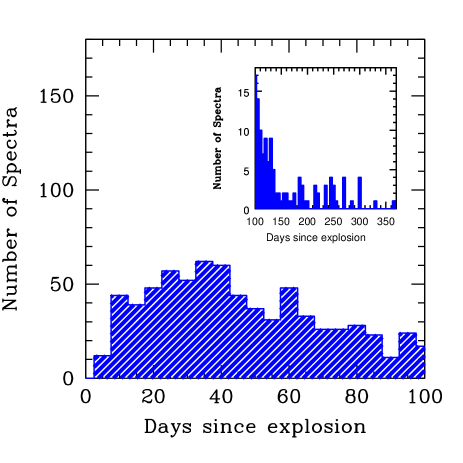
Figure 5.— Distribution of the number of spectra as a function of epoch from explosion. The inset on the right shows the same distribution between 100 and 370 days.

Figure 6 shows the epoch distribution of the first and last spectrum for each SN in our sample. The majority of SNe have their first spectra within 40 days from explosion. There are 31 SNe with their first spectra around 10 days (the peak of the distribution). On the other hand, the peak of the distribution of the last spectrum is around 100 days. Almost all SNe have their last spectra between 30 and 120 days, i.e., in the photospheric phase. There are 11 SNe with their last spectrum after 140 days, while only 4 SNe (SN 1993K, 2003B, SN 2007it, SN 2008bk) have their last spectrum in the nebular phase ($\geq 200$ days).

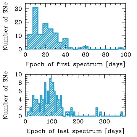
Figure 6.— Top: Epoch from explosion of first spectrum. Bottom: Epoch from explosion of last spectrum.

The photometric behaviour of our sample in terms of their plateau decline rate (s₂; defined in Anderson et al. 2014b) in the $V$ band is shown in Figure 7. For our sample of 117 SNe II, we measure $s_{2}$ values ranging between $-0.76$ and 3.29 mag 100d^-1. Higher $s_{2}$ values mean that the SN has a faster declining light curve. We can see a continuum in the s₂ distribution, which shows that the majority of the SNe (83) have a s₂ value between 0 and 2. There are 8 objects with s₂ values smaller than 0, while 3 SNe show a value larger than 3. The average of s₂ in our sample is 1.20. We are unable to estimate the s₂ value for 5 SNe as there is insufficient information from their light curves. The s₂ distribution for the 22 SNe II used as new templates in SNID is also shown in Figure 7. Although the diversity in the SNID templates increased with the inclusion of these SNe, the template distribution is still biased to low $s_{2}$ values.

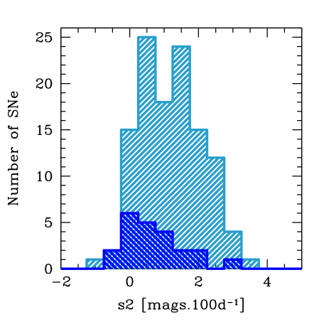
Figure 7.— Distribution of the plateau decline s₂ in $V-$band for 117 SNe of our sample. The blue histogram presents the distribution of “s₂” in $V-$band for 22 SNe II used as a new template in SNID

.

VI. Spectral line identification

We identified 20 absorption features within our photospheric spectra, in the observed wavelength range of 3800 to 9500 Å. Their identification was performed using the Atomic Spectra Database and theoretical models (e.g. Dessart & Hillier, 2005, 2006, 2011). Early spectra exhibit lines of H_α $\lambda 6563$, H_β $\lambda 4861$, H_γ $\lambda 4341$, H_δ $\lambda 4102$, and He I $\lambda 5876$, with the latter disappearing at $\sim 20-25$ days past explosion. An extra absorption component on the blue side of H_α (hereafter “Cachito” is present in many SNe). That line has previously been attributed to high velocity (HV) features of hydrogen or Si II $\lambda 6533$. Figure 8 shows the main lines in early spectra of SNe II at 3 and 7 days from explosion. We can see that SN 2008il shows the Balmer lines and He I, while SN 2007X, in addition to these lines, also shows Cachito on the blue side of H_α.

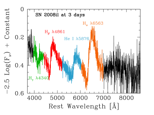
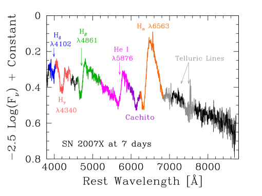
Figure 8.— Line identification in the early spectrum of SN 2008il (top) and SN 2007X (bottom).

In Figure 9 we label the lines present in the spectra of SNe II during the photospheric phase at 31, 70 and 72 days from explosion. Later than $\sim 15$ days the iron group lines start to appear and dominate the region between 4000 and 6000 Å. We can see Fe-group blends near $\lambda 4554$, and between 5200 and 5450 Å (where we refer to the latter as “Fe II blend” throughout the rest of the text). Strong features such as Fe II $\lambda 4924$, Fe II $\lambda 5018$, Fe II $\lambda 5169$, Sc II/Fe II $\lambda 5531$, the Sc II multiplet $\lambda 5663$ (hereafter “Sc II M”), Ba II $\lambda 6142$, Sc II $\lambda 6247$, O I $\lambda 7774$, O I $\lambda 9263$ and the Ca II triplet $\lambda\lambda 8498,8662$ ($\lambda 8579$) are also present from $\sim 20$ days to the end of the plateau. At 31 days, SN 2003hn shows all these lines, except Ba II, while at 70 and 72 days, SN 2003bn and SN 2007W show all the lines. Unlike SN 2003bn, SN 2007W shows Cachito and the “Fe line forest”. The Fe line forest is visible in a small fraction of SNe from 25-30 days (see the analysis in section VIII). As we can see there are significant differences between two different SNe at almost the same epoch. Later we analyze and discuss how these differences can be understood in terms of overall diversity of SN II properties.

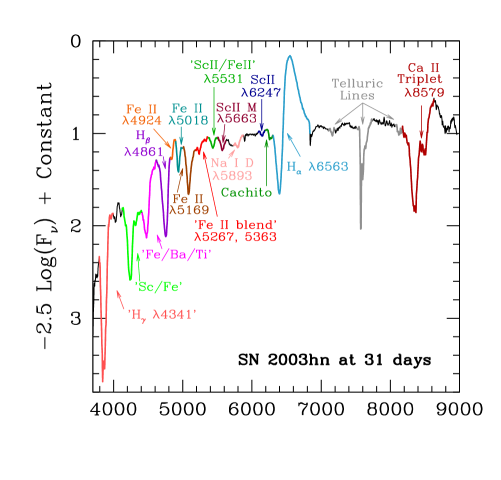
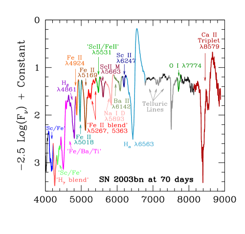
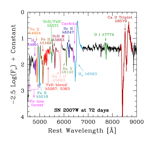
Figure 9.— Line identification in the photospheric phase for SNe II 2003hn at 31 days (top), 2003bn at 70 days (middle), and 2007W at 72 days (bottom).

In the nebular phase, later than 200 days post explosion, the forbidden lines [Ca II] $\lambda\lambda 7291,$ 7323, [O I] $\lambda\lambda 6300,$ 6364 and [Fe II] $\lambda 7155$ emerge in the spectra. At this epoch H_α, H_β, Na I D, the Ca II triplet, O I and the Fe group lines between 4800 and 5500 Å, and 6000-6500 Å are also still present. Figure 10 shows a nebular spectrum of SN 2007it at 250 days from explosion.

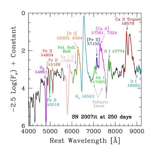
Figure 10.— Line identification in the nebular spectrum of SN II 2007it at 250 days from explosion.

VI.1. The H_α P-Cygni profile

H_α $\lambda 6563$ is the dominant spectral feature in SNe II. It is usually used to distinguish different SN types using the initial spectral observation. This line is present from explosion until nebular phases, showing, in the majority of cases, a P-Cygni profile. Although the P-Cygni profile has an absorption and emission component, SNe display a huge diversity in the absorption feature.

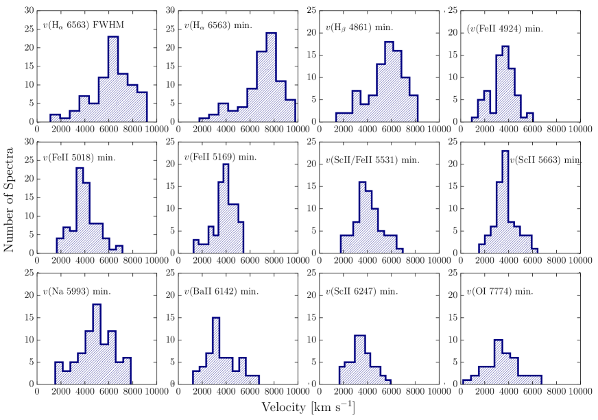
Figure 11.— Distribution of the expansion ejecta velocities for 11 optical features at 50 days. The first two panels show the H_α velocity obtained from the FWHM and from the minimum absorption flux. From third to twelfth panel are presented the H_β, Fe II $\lambda 5018$, Fe II $\lambda 4924$, Fe II $\lambda 5169$, Sc II/Fe II $\lambda 5531$, Sc II $\lambda 5663$, Na I D $\lambda 5893$, Ba II $\lambda 6142$, Sc II $\lambda 6247$, O I $\lambda 7774$ velocities obtained from the minimum absorption flux

.

Gutiérrez et al. (2014) showed that SNe with little absorption of H_α (smaller absorption to emission ($a/e$) values) appear to have higher velocities, faster declining light curves and tend to be more luminous. Here we show H_α displays a large range of velocities in the photospheric phase, from 9500 km s^-1 to 1500 km s^-1 at 50 days (see the first two panels in Figure 11, which correspond to the H_α velocity derived from the FWHM of the emission component and from the minimum flux of the absorption, respectively).
The diversity of H_α in the photospheric phase is also observed through the blueshift of the emission peak at early times (Dessart & Hillier, 2008; Anderson et al., 2014a) and the boxy profile (Inserra et al., 2011, 2012). The former is associated with differing density distributions of the ejecta, while the latter with an interaction of the ejecta with a dense CSM. In the nebular phase this shift in H_α emission peak has been interpreted as evidence of dust production in the SN ejecta. Despite the fact that this is an important issue in SNe II, only a few studies (e.g. Sahu et al., 2006; Kotak et al., 2009; Fabbri et al., 2011) have focussed on these features.
In Figure 12 we show an example of the evolution of H_α P-Cygni profile in SN 1992ba. We can see in early phases a normal profile which evolves to a complicated profile around 65 days. Cachito on the blue side of H_α is present from 65 to 183 days.

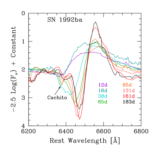
Figure 12.— H_α P-Cygni profile evolution in SN 1992ba. The epochs are labeled on the right.

VI.2. H_β, H_γ and H_δ absorption features

H_β $\lambda 4861$, H_γ $\lambda 4341$ and H_δ $\lambda 4102$ like H_α are present from the first epochs. In earlier phases, these lines show a P-Cygni profile, however, from $\sim 15$ days the spectra only display the absorption component, giving space to Fe group lines. The range of velocities of H_β, H_γ and H_δ at 50 days post explosion vary from 8000 to 1000 km s^-1 (see Figure 11).
Although H_δ is a common line in SNe II, we do not include a detailed analysis of this line because in many cases the spectra are noisy in the blue part of the spectrum. Besides, like other lines in the blue, this line is blended with Fe-group lines later than 30 days.
Around 30 days from explosion H_γ starts to blend with other lines, such as Ti II and Fe II. Meanwhile in a few SNe, the H_β absorption feature is surrounded by the Fe line forest. Our later analysis shows that SNe displaying this behaviour are generally dimmer and lower velocity events (see Section VIII for more details).

VI.3. He I $\lambda 5876$ and Na I D $\lambda 5893$

He I $\lambda 5876$ is present in very early phases when the temperature of the ejecta is high enough to excite the ground state of helium. As the temperature decreases, the He I line starts to disappear due to low excitation of He I ions (around 15 days; Roy et al. 2011; Dessart & Hillier 2010). At $\sim 30$ days the Na I D $\lambda 5893$ absorption feature arises in the spectrum at a similar position where He I was located. This new line evolves with time to a strong P-Cygni profile, displaying velocities between 8000 km s^-1 to 1500 km s^-1 at 50 days from explosion (Figure 11).
In many SNe II (or indeed SNe of all types), at these wavelengths one often observes narrow absorption features arising from slow-moving line of sight material from the interstellar medium, ISM (or possibly from circumstellar material, CSM). Such material can constrain the amount of foreground reddening suffered by SNe, however we do not discuss this here.

VI.4. Fe-group lines

When the SN ejecta has cooled sufficiently, Fe II features start to dominate SNe II spectra between 4000 to 6500 Å. The first line that appears is Fe II $\lambda 5169$ on top of the emission component of H_β. With time Fe II $\lambda 5018$ and $\lambda 4924$ emerge between H_β and Fe II $\lambda 5169$. Fe II $\lambda 5169$ becomes a Fe II blend later than $\sim 30-40$ days. At $\sim 50$ days the 4000-5500 Å region is completely filled with these lines and the continuum is diminished due to Fe II line-blanketing. The H_γ and H_δ absorption features are blended with Fe-group lines, such as Fe II, Ti II, Sc II and Sr II. Between $\sim 5400$ and 6500 Å other metal lines appear in the spectra. Lines such as Sc II/Fe II $\lambda 5531$, Sc II M, Ba II $\lambda 6142$ and Sc II $\lambda 6247$ get stronger with time.
As we can see in Figure 11, the Fe-group lines show a range of velocities between 7000 km s^-1 to 500 km s^-1 at 50 days. The peak of the distribution of the Fe II group lines velocities is around 4000 km s^-1. In the case of Ba II, the peak is lower (around 3000 km s^-1).
Although Fe II lines always appear at late phases, few SNe show the iron line forest at 30 days. This feature appears earlier in low velocity/luminosity SNe (See section VIII).

VI.5. The Ca II NIR triplet

The Ca II NIR triplet is a strong feature in the spectra of SNe II. This line appears at $\sim 20-30$ days as an absorption feature, but with time it starts to show an emission component. The Ca II NIR triplet results in a blend of $\lambda$8498 and $\lambda$8542 in the bluer part and a distinct component, $\lambda$8662 on the red part. In SNe II with higher velocities these lines are blended producing a broad absorption and emission profile, however, in low-velocity SNe, we see two absorption components and one emission in the red part. The velocities of the Ca II NIR triplet range between 9000 to 1000 km s^-1 at 50 days. In the nebular phase the Ca II NIR triplet is also present, however at this epoch it only exhibits the emission component.
Although in the majority of our spectra we can not see Ca II H & K $\lambda 3945$, due to the poor signal to noise in this region, this line is present in the photospheric phase of SNe II.
While the Ca II NIR triplet is a prominent feature in SNe II, we do not include its analysis in the subsequent discussion, given that the overlap of lines makes a consistent comparison of velocities and pseudo-equivalent widths (pEWs) difficult.

VI.6. O I lines

The O I $\lambda\lambda 7772$, 7775 doublet (hereafter O I $\lambda 7774$) and O I $\lambda 9263$ are the oxygen lines in the optical spectra of SNe II. These lines are mainly driven by recombination and they appear when the temperature decreases sufficiently. The O I $\lambda 7774$ line is relatively strong and emerges around 20 days from explosion, however in the majority of cases it is contaminated by the telluric A-band absorption ($\sim 7600-7630$ Å), which hinders detailed analysis. O I $\lambda 9263$ is weaker and appears one month later than O I $\lambda 7774$. These lines are present until the nebular phase and their expansion velocity at 50 days post explosion goes from $\sim 7000$ km s^-1 to 500 km s^-1, as can be seen in Figure 11.

VI.7. Cachito: Hydrogen High Velocity (HV) Features or the Si II $\lambda$6355 line?

The extra absorption component on the blue side of H_α P-Cygni profile, called here “Cachito”, is seen in early phases in some SNe (e.g. SN 2005cs, Pastorello et al. 2006; SN 1999em, Baron et al. 2000) as well as in the plateau phase (e.g. SN 1999em, Leonard et al. 2002b SN 2007od, Inserra et al. 2011). However, its shape and strength is completely different in the two phases. Baron et al. (2000) assigned the term “complicated P-Cygni profle” to explain the presence of this component on the blue side of the Balmer series. They concluded that these features are due to velocity structures in the expanding ejecta of the SNe II. A few years later, Pooley et al. (2002) and Chugai et al. (2007) argued that this extra component might originate from ejecta – circumstellar (CS) interactions, while Pastorello et al. (2006) earmarked this feature as Si II $\lambda 6355$.
In general, Cachito appears around 5-7 days between 6100 and 6300 Å, and disappears at $\sim 35$ days after explosion. Later than 40 days the Cachito feature emerges closer to H_α (between 6250-6450 Å) and it can be seen until 100-120 days. Figure 13 shows this component in SN 2007X. In early phases this feature is marked with letter A and later with letter B. If attributed to H_α the derived velocities are 18000 km s^-1 and 10000 km s^-1, respectively. A detailed analysis of this feature is presented in VIII.4.

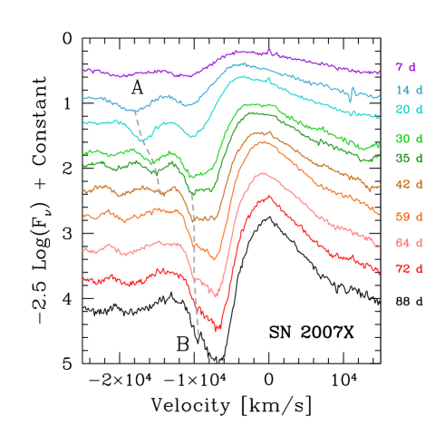
Figure 13.— H_α P-Cygni profile of the SN 2007X. The epochs are labeled on the right. The dashed lines indicate the velocities for the A and B features, which we call ‘Cachito’.

VI.8. Nebular Features

As mentioned above, H_α, H_β, the Ca II NIR triplet, Na ID , O I and Fe II are also present in the nebular phase (later than 200 days since explosion), however in the case of the Ca II NIR triplet, its appearance changes, passing from absorption and emission components to only emission components when the nebular phase starts. The rest of the lines have the same behaviour but at much later epochs. The emergence of forbidden emission lines signifies that the spectrum is now forming in regions of low density. At this phase, the ejecta has become transparent, allowing us to peer into the inner layers of the rapidly expanding ejecta. Lines such as [Ca II] $\lambda\lambda 7291,$ 7323, [O I] $\lambda\lambda 6300,$ 6364 and H_α are the strongest features visible in the spectra.
The [O I] doublet observed at nebular times is one of the most important diagnostic lines of the helium-core mass (Fransson & Chevalier, 1987; Jerkstrand et al., 2012). Usually the doublet is blended, however in SNe with low velocities these lines can be resolved (see e.g. SN 2008bk). On the other hand, [Fe II] $\lambda 7155$ is easily detectable, but in most cases it is blended with [Ca II] $\lambda\lambda 7291,$ 7323 and He I $\lambda 7065$, which may hinder their analysis. In Figure 14 we can see the diversity found in the nebular spectra in our sample.

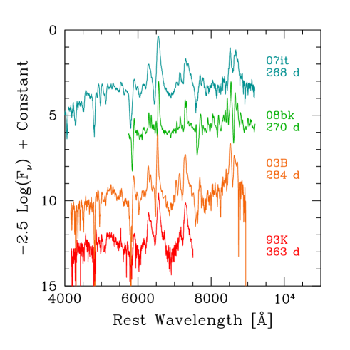
Figure 14.— Nebular spectra of seven different SNe of our sample. The spectra are organized according to epoch.

VII. Spectral measurements

As discussed previously, SNe II spectra evolve from having a blue continuum with a few lines (Balmer series and He I) to redder spectra with many lines: Fe II, Ca II, Na I D, Sc II, Ba II, and O I. To analyze the spectral properties of SNe II, we measure the expansion velocities and pEWs of eleven features in the photospheric phase (see in Table 3 the features used), the ratio of absorption to emission ($a/e$) of H_α P-Cygni profile before 120 days, and the velocity decline rate of H_β.

VII.1. Expansion ejecta velocities

The expansion velocities of the ejecta are commonly measured from the minimum flux of the absorption component of the P-Cygni line profile. Using the Doppler relativistic equation and the rest wavelength of each line, we can derive the velocity. To obtain the position of the minimum line flux (in wavelength), a Gaussian fitting was employed, which was performed with IRAF using the splot package. As the absorption component presents a wide diversity (e.g. asymmetries, flat shape, extra absorption components) we repeat the process many times (changing the pseudo-continuum), and the mean of the measurements was taken as the minimum flux wavelength. As our measurement error we take the standard deviation on the measurements. This error is added in quadrature to errors arising from the spectral resolution of our observations (measured in Å and converted to km s^-1) and from peculiar velocities of host galaxies with respect to the Hubble flow (200 km s^-1). This means that, in addition to the standard deviation error, which realizes the width of the line and $S/N$, we take into account the spectral resolution, that in our case is the most dominant parameter to determine the error.
The particular case of the H_α velocity was explored in Gutiérrez et al. (2014). Due to the difficulty of measuring the minimum flux in a few SNe with little or extremely weak absorption component, we derive the expansion velocity of H_α using both the minimum flux of the absorption component and the full-width-at-half-maximum (FWHM) of the emission line.
In the case of O I $\lambda$ 7774 where the telluric lines can affect our measurement of its absorption minimum, we only use SNe with a clear separation between the two features. This means that the number of SNe with O I measurements is significantly smaller (only 47 SNe) compared to the other measured features.

VII.2. Velocity decline rate

To calculate the time derivative of the expansion velocity in SNe II, we select the H_β absorption line. It is present from the early spectra, it is easy to identify and it is relatively isolated. To analyze quantitatively our sample, we introduce the $\Delta v($H${}_{\beta})$ as the mean velocity decline rate in a fixed phase range [t₀,t₁]:

$\Delta v($H${}_{\beta})=\frac{\Delta v_{abs}}{\Delta t}=\frac{v_{abs}(t_{1})-v_{abs}(t_{0})}{t_{1}-t_{0}}$.

This parameter was measured over the interval [+15,+30] d, [+15,+50] d, [+30,+50] d, [+30,+80] d, and [+50,+80] d.

VII.3. Pseudo-equivalent widths

To quantify the spectral properties of SNe II, another avenue for investigation is the measurement and characterization of spectral line pEWs. The prefix “pseudo” is used to indicate that the reference continuum level adopted does not represent the true underlying continuum level of the SN, given that in many regions the spectrum is formed from a superposition of many spectral lines. The pEW basically defines the strength of any given line (with respect to the pseudo-continuum) at any given time. The simplest and most often used method is to draw a straight line across the absorption feature to mimic the continuum flux. Figure 15 shows an example of this technique applied to SN 2003bn. We do not include analysis of spectral lines where it is difficult to define the continuum level, due to complicated line morphology, such as significant blending between lines. For example, later than 20 - 25 days all absorption features bluer than H_β are produced by blends of Fe-group lines plus other strong lines, such as Ca II H & K and H_γ. On the other hand, the Ca II NIR triplet $\lambda\lambda 8498$, 8662 shows a profile that depends on the SN velocity (higher velocity SNe show a single broad absorption, while low velocity SNe show two absorption characteristics). These attributes make a consistent analysis between SNe difficult, and therefore we do not include this line in our analysis.

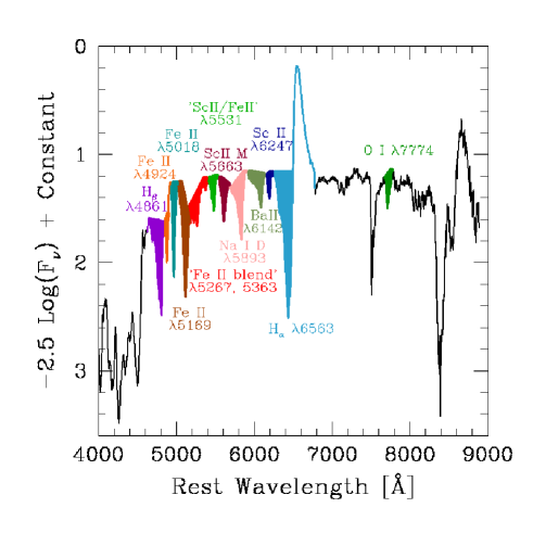
Figure 15.— Examples of pEWs used in this work for eleven features in the photospheric phase of SN 2003bn (at 70 days).

We measure the ratio of absorption to emission ($a/e$) in H_α until 120 days. In the same way the pEWs of the absorption lines are measured, we evaluate the pEWs for the emission in H_α, thus we have:

$a/e=\frac{pEW(H_{\alpha(abs)})}{pEW(H_{\alpha(emis)})}$.

VIII. Line Evolution analysis

Here we study the time of appearance of different lines within different SNe, and make a comparison of those SNe with/without specific lines at different epochs. For all lines included in our analysis, we search for their presence in each observed spectrum. Then, at any given epoch we obtain the percentage of SNe that display each line. This enables an analysis of the overall line evolution of our sample and whether the speed of this evolution changes between different SNe of different light curve, spectral, and environment (metallicity) characteristics.
In Figure 16 we show the percentage of SNe displaying specific spectral features as a function of time. As discussed previously, H_α and H_β are permanently present in all the SNe II spectra from the first days, so we do not include them in the plot. We can see that:

• The feature located in the position of He I/Na I D is visible in all epochs, however around 15-25 days fewer SNe show the line respect to either earlier or later spectrum. We suggest that in this epoch the transition from He I to Na I D happens. Therefore, after 30 days we refer to this line as Na I D. It is present in 96% of the spectra from $\sim 35$ days. Later than 43 days it is present in all spectra.

• The Ca II NIR triplet is present in $50\%$ of the sample at $\sim 20$ days. Before 20 days it is present in $\sim 12\%$ of the sample, while later than 25 days is visible in almost all the sample, but with one exception at 38 days. The latter is SN 2009aj, which shows signs of CS interaction in the early phases.

• H_γ blend with Fe-group lines starts at $\sim 20$ days from explosion, growing dramatically at 35-45 days. Only one spectrum at $\sim 46$ days does not show the blend (SN 2008bp).

• The Fe-group lines start to appear at around 10 days (see Figure 16). The first line that emerges is Fe II $\lambda 5169$. We can see that few SNe exhibit the absorption feature before 15 days, however later at 15 days around 50% of SNe show the line and at 30 days all objects have it. The next line that arises is Fe II $\lambda 5018$. This line is seen from 15 days, being present in all SNe later than 40 days. Meanwhile, Fe II $\lambda 4924$ is seen in one spectrum at 13 days (SN 2008br). From 30 days it is visible in more than 50% of the spectra. The Sc II/Fe II $\lambda 5531$, Sc II multiplet $\lambda 5668$, Ba II $\lambda 6142$ and Sc II $\lambda 6246$ are detectable later than 30 days. The emergence of the Sc II/Fe II $\lambda 5531$ and Sc II multiplet $\lambda 5668$ happens at similar epochs, as well as Ba II $\lambda 6142$ and Sc II $\lambda 6246$.

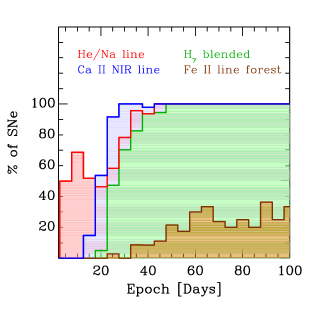
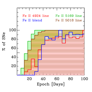
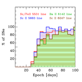
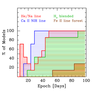
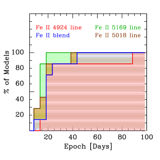
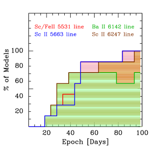
Figure 16.— Appearance of different lines in SNe II between explosion and 100 days. Top: from the observed spectra. Bottom: from synthetic spectra (see more details in Table 5).

In order to further understand the differences in line-strength evolution of SNe II, we separate the sample into those SNe that do/do not display a certain spectral feature at some specific epoch. We then investigate whether these different samples also display differences in their light-curves and spectra. This is done by using the Kolmogorov-Smirnov (KS) test. Presented in Table 4 are all the results obtained with KS test: SNe with/without a given line as a function of $a/e$ and H_α velocity at t_tran+10, M_max, s₂, and metallicity (derived from the ratio of H_α to [N II] $\lambda 6583$, henceforth M13 N2 diagnostic; Marino et al. 2013) in a particular epoch. The values of the first four parameters can be found in Table 1 in Gutiérrez et al. (2014), while the metallicity information was obtained from Anderson et al. (2016). We find that:

• SNe II that never display the Fe II line forest are distinctly different from those that do display the feature. Specifically, those that do show this feature have slow declining light curves (smaller s₂), are dimmer, and are found to explode in higher metallicity regions within their hosts (see Table 4 for exact statistics).

• There is less than a 2% probability that those SNe II where the He I line is detected between 18 and 22 days post explosion arise from the same underlying parent population of $a/e$. This suggests that temperature differences between SNe II affect the morphology of the H_α feature.

• Ba II $\lambda$6142 and Sc II $\lambda$6247 are both more likely to be detected at around 40 days post explosion in dimmer SNe II, with only a  2% probability that the two populations (with and without these lines) are drawn from the same M_max distribution.

• Finally, when splitting the SNe II sample into those that do and do not display: Sc II/Fe II $\lambda 5531$, Sc II multiplet $\lambda 5668$, Ba II $\lambda$6142 and Sc II $\lambda$6247 at around 40 days post explosion we find that there is only around a 1% probability that the two samples are drawn from the same distribution of metallicity: those SNe that do not display these lines at this epoch are found to generally explode in regions of lower metallciity within their hosts

Figure 17 presents the cumulative distributions of the most significative findings obtained with the KS-test analysis.

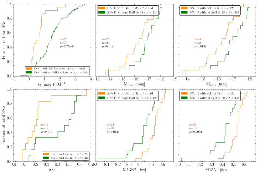
Figure 17.— Cumulative distributions of each SN with/without different lines as a function of spectral and photometric and environment properties. First panel: SNe with/without Fe II line forest between explosion and 100 days as a function of s₂; second panel: SNe with/without Ba II between 38 and 42 days as a function of M_max; third panel: SNe with/without Sc II between 38 and 42 days as a function of M_max; fourth panel: SNe with/without He I between 18 and 22 days as a function of $a/e$; fifth panel: SNe with/without Ba II between 38 and 42 days as a function of M13N2 diagnostic; sixth panel: SNe with/without Sc II between 38 and 42 days as a function of M13N2 diagnostic.

This analysis was also performed with synthetic spectra for seven different models from Dessart et al. (2013). Four models (m15z2m3, m15z8m3, m15z8m3, m15z4m2) show differences in the metallicity, while the rest of the properties are almost the same. The three remaining models have the same metallicity (solar metallicity), however the other parameters are different: m15mlt1 has a bigger radius (twice times the radius of the two other models), m15mlt3 has higher kinetic energy, while m12mlt3 displays a smaller final progenitor mass and less kinetic energy (1/5 E_kin compared with the other models). More details are shown in Table 5.
In general, the synthetic spectra show the same behaviour (in relation to the appearance of the lines) as observed spectra. However, some differences are found, the majority of which are probably related with the low area of parameter space covered by the models that currently exist as compared to the parameter space covered by real events. The transition between He I to Na I D is more evident, and it happens between 18 and 40 days. Although the transition in the models is unambiguously identified by knowing the optical depth of specific lines, in these synthetic spectra this happens a little bit later than in observed ones. This suggests the temperature in specific models stays higher for a longer time than the average for observed SNe II. It is also likely that the observed SNe II span a smaller range in progenitor metallicity than the models (that go down to a tenth solar). The Na I D is visible in 100% of the sample after 50 days, only 5 days later than the observed spectra. Ca II shows the same behaviour in both synthetic and observed spectra, however H_γ is blended in all of the sample later than 90 days, unlike the observed spectra that show it from 45 days. On the other hand, the Fe II line forest is visible from 55 days, in contrast to the observed spectra that show this characteristic from 30 days. This behaviour is only present in the spectra of higher metallicity model (2 times solar) and in the lower explosion energy model. The iron lines (Fe II $\lambda 4924$, Fe II $\lambda 5018$, Fe II $\lambda 5169$, and the Fe II blended) are present from $\sim 10$ days. Fe II $\lambda 5169$ is visible in 50% of the spectra at $\sim 15$ days, while Fe II $\lambda 4924$ is only visible in $\sim 10$%. From 20 days Fe II $\lambda 5169$ is present in all the synthetic spectra, 10 days before than in the observed ones. The behaviour of Fe II $\lambda 5018$ is similar in both synthetic and observed spectra, whereas Fe II $\lambda 4924$ starts faster in the models and it is visible in 85% of the spectra from 30 days. We can see differences in the Fe II blend, which is visible in 100% of the sample from 50 days in the models, however in the observed spectra that never happens. More differences are also appreciable between models and observation in Sc II/Fe II $\lambda 5531$, the Sc II multiplet $\lambda 5668$, Ba II $\lambda 6142$ and Sc II $\lambda 6246$. These lines in models arise from 20 days, but in the observations it occurs from 38-40 days. Nevertheless, the evolution of the distribution is similar from 50 days. In conclusion, while in general the models produce a time evolution of spectral lines that is quite similar to the observations - supporting the robustness of the models - we observe small differences, suggesting a wider range of explosion and progenitor properties is required to explain the full diversity of observed SNe II.

VIII.1. Expansion velocity evolution

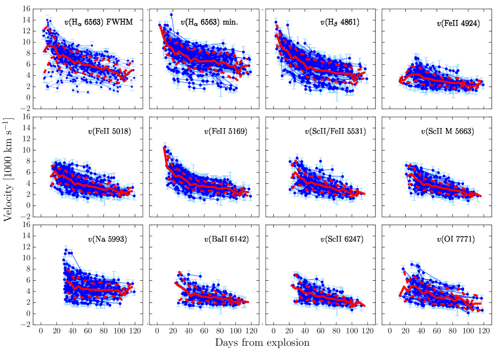
Figure 18.— Expansion velocity evolution for H_α (from the FWHM of emission and the minimum flux absorption), H_β, Fe II $\lambda 4924$, Fe II $\lambda 5018$, Fe II $\lambda 5169$, Sc II/Fe II, Sc II multiplet, Na I D, Ba II, Sc II and O I from explosion to 120 days. The red solid line represents the mean velocity within each time bin, while the dashed red lines indicate the standard deviation. Table A3 presents these values.

Figure 18 shows the velocity evolution of eleven spectral features as a function of time. The first two panels of the plot show the expansion velocity of the H_α feature: on the left the velocity derived from the FWHM and on the right that derived from the minimum absorption flux. As we can see, the behaviour is similar, however the velocity obtained from the minimum absorption flux is offset between 10 and 20% to higher velocities. Figure 19 shows this shift at 50 days. Velocities obtained from the minimum absorption flux are higher around $\sim 1000$ km s^-1. However, it is possible to see few SNe (with higher H_α velocities) showing higher values from the FWHM. Using the Pearson correlation test we find a weak correlation, with a value of $\rho=0.37$. SNe II with narrower emission components display a larger offset between the velocity from the FWHM and that from the minimum of the absorption. In contrast, those SNe II displaying the highest FWHM velocities present comparatively lower minimum absorption velocities. We note also the presence of two outliers (extreme cases, the lowest and highest value). Figure 11 shows the velocity distribution for the eleven features at 50 days post explosion. We can see that H_α shows higher velocities than the other lines, followed by H_β. The lowest velocities are presented by the iron-group lines. In Figure 18 it is possible to see that the H_β expansion velocity shows the typical evolution for a homologous expansion and like H_α, it is possible to see it from early phases. The iron lines display lower velocities than the Balmer lines. So, the highest velocity in SNe II is found in H_α, which implies that it is formed in the outer layers of the SN ejecta. Meanwhile, based on the lower velocities, the iron-group lines form in the inner part, closer to the photosphere. The O I line does not show a strong evolution. As we can see, its velocity evolution is almost flat.
The lowest velocities are found in SN 2008bm, SN 2009aj and SN 2009au. However, these SNe are distinct from the rest of the population. Unlike sub-luminous SNe II (such as SN 2008bk and SN 1999br) – that also display low expansion velocities – these events are relatively bright. They also show early signs of CS interactions, e.g., narrow emission lines. By contrast, SN 2007ab, SN 2008if and SN 2005Z have the largest velocities.

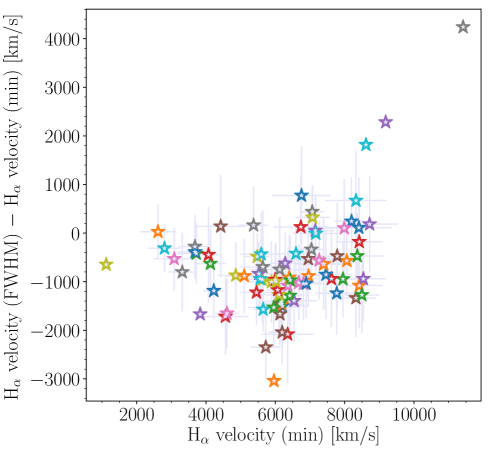
Figure 19.— Shifts of the H_α velocity obtained form the FWHM of the emission and from the minimum of the absorption at 50 days post explosion.

VIII.2. Velocity decline rate of H_β analysis

The velocity decline rate of SNe II, denoted $\Delta v($H_β), has not been previously analyzed. We estimate $\Delta v($H${}_{\beta})$ in five different epochs (outlined above) to understand their behaviour. We find that SNe with a higher decline rate at early times continue to show such behaviour at later times. The median velocity decline rate for our sample between 15 and 30 days is 105 km $s^{-1}$ d^-1, while between 50 and 80 days is 29 km $s^{-1}$ d^-1. This results show an evident decrease in the velocity decline rate at two different intervals, which is consitent with homologous expansion.

VIII.3. pEWs evolution

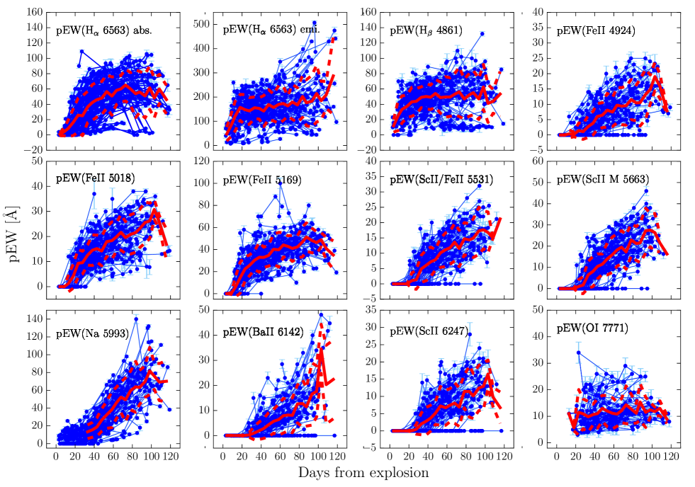
Figure 20.— pEWs evolution for H_α absorption, H_α emission, H_β, Fe II $\lambda 4924$, Fe II $\lambda 5018$, Fe II $\lambda 5169$, Sc II/Fe II, Sc II multiplet, Na I D, Ba II, Sc II and O I from explosion to 120 days. The red sold line represents the mean pEW within each time bin, while the dashed red lines indicate the standard deviation. Table A4 presents these values.

The temporal evolution of pEWs for each of the eleven spectral features is shown in Figure 20. In general the pEWs increase quickly in the first 1-2 months then level off. The first two panels show the pEW evolution of H_α. On the left is displayed the absorption, while on the right the emission component. The absorption component monotonically increases from 0 increasing to $\sim 100$ Å, however in a few SNe its evolution is different: from 70 days the pEW decreases significantly. This behaviour is observed in low and intermediate velocity SNe (e.g., SN 2003bl, SN 2006ee, SN 2007W, SN 2008bk, SN 2008in and SN 2009N). Generally, these SNe show a very narrow H_α P-cygni profile, and at around 70 days from explosion Ba II $\lambda 6497$ appears in the spectra as a dominant feature (see Roy et al. 2011; Lisakov et al. 2017 for more details). In Figure 21 we can see the H_α P-Cygni profile with the presence of Ba II $\lambda 6497$, and the HV feature of hydrogen line (see section VIII.4 for more details) on the blue side of Ba II.
Figure 20 also shows the H_α emission component evolution. An increment in the pEW in the majority of SNe is appreciable. There are a couple cases (e.g. SN 2006Y), displaying a quasi-constant evolution. The range of pEW of H_α emission goes up 400 Å. In the case of H_β, we can see that from 60 days there are few SNe with low pEW values, which show a quasi-constant evolution. SNe with this behaviour are those that show the Fe II line forest. The remaining SNe show an increase. The pEWs of iron-group lines grow with time, however there is a group of SNe with pEW$=0$. This indicates that some specific SNe do not have the line yet. For Sc II/Fe II, the Sc II multiplet, Ba II, and Sc II this is more obvious. On the other hand, the O I shows a quasi-constant behaviour and Na I D a steady increase. Comparing the values, we can see that the absorption of H_α, H_β and Na I D have the highest values (from 0 to $\sim 120$), while Fe II $\lambda 4924$, Fe II $\lambda 5018$, Sc II/Fe II, the Sc II multiplet, Ba II, Sc II and O I have the lowest ones (from 0 to $\sim 50$).

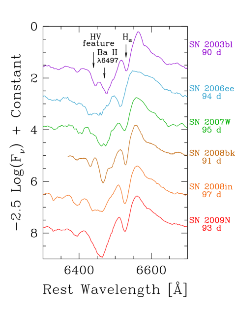
Figure 21.— H_α P-Cygni profile of low and intermediate velocity SNe II: 2003bl, 2006ee, 2007W, 2008bk, 2008in and 2009N around 95 days post-explosion.

The $a/e$ evolution is displayed in Figure 22. One can see an increase until $\sim 60$ days and then, the quantity remains constant or slightly decreases.

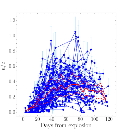
Figure 22.— Evolution of the ratio absorption to emission ($a/e$) of H_α between explosion and 120 days.

VIII.4. Cachito: Hydrogen HV features or Si II line

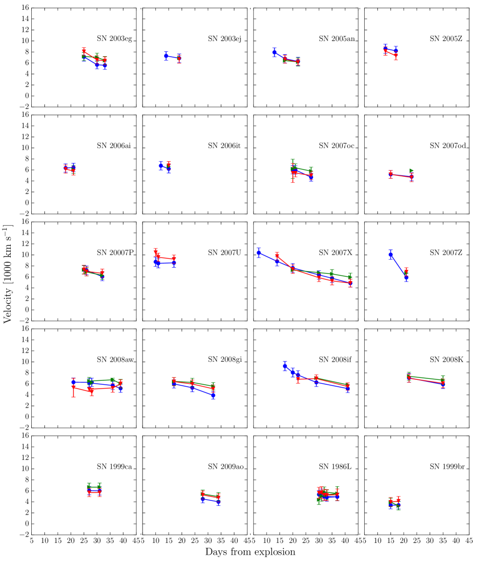
Figure 23.— Velocity evolution of Cachito (blue) at early phases compared with Fe II $\lambda$5018 (green) and Fe II $\lambda$5169 (red).

The nature of Cachito has recently been studied. Its presence on the blue side of H_α has given rise to multiple interpretations, such as HV features of hydrogen (e.g. Leonard et al., 2002b; Baron et al., 2000; Chugai et al., 2007; Inserra et al., 2011) or Si II $\lambda 6355$ (e.g. Pastorello et al., 2006; Valenti et al., 2013; Tomasella et al., 2013). Seventy SNe from our sample show Cachito in the photospheric phase, between 7 and 120 days post-explosion, however its behaviour, shape and evolution is different depending on the phase. To investigate the nature of Cachito we examine the following possibilities:

• If Cachito is produced by Si II its velocity should be similar to those presented by other metal lines.

• If Cachito is related to HV features of hydrogen, its velocity should be almost the same as those obtained from H_α at early phases. In addition, if it is present, a counterpart should be visible on the blue side of H_β.

Analyzing our sample we can detect Cachito in 50 SNe at early phases (before 40 days). Because of the high temperatures at these epochs, the presence of Ba II $\lambda 6497$ is discarded. Assuming that Cachito is produced by Si II, we find that 60% of SNe present a good match with Fe II $\lambda 5018$ and Fe II $\lambda 5169$ velocities. Conversely, the rest of the sample shows velocities comparable to those measured at very early phases for H_α. Curiously the Cachito shape is different between the two SN groups. In the former, the line is deeper and broader, while in the latter, the line is shallow. In Figure 23 we present the velocity comparison for the former group, where a good agreement is found between Cachito, assumed as Si II $\lambda 6355$ (blue), and the iron lines, Fe II $\lambda 5018$ (green) and Fe II $\lambda 5169$ (red).

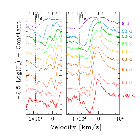
Figure 24.— Spectral evolution of H_α and H_β lines of SN 2004fc. The dotted lines correspond to the HV features seen on the blue side of H_α and H_β from 50 to 120 days. We can see that the HV features show a velocity evolution from $\sim 9000$ to $\sim 8000$ km s^-1.

Later than 40 days we detect Cachito in 43 SNe. Proceeding with the velocity comparison, we can discard its identification as Si II or Ba II $\lambda 6497$ (the latter, visible in few SNe from 60 days, see Figure 21), which suggests that Cachito is associated to hydrogen. During the plateau it is possible to see Cachito as a shallow absorption feature only in H_α and/or as a narrow and deeper absorption on the blue side of both H_α and H_β (see an example in Figure 24). According to Chugai et al. (2007), the interaction between the SN ejecta and the RSG wind should result in the emergence of these HV absorption features. They argue that the existence of a shallow absorption feature is the result of the enhanced excitation of the outer unshocked ejecta, which is visible on the blue side of H_α (and He I $\lambda$10830). At early times the H_β Cachito feature is not predicted by Chugai et al. (2007), who argue that the optical depth is too low at the line forming region. They also discuss that in addition to the HV shallow absorption, a HV notch is formed in the cool dense shell (CDS) located behind the reverse shock. Given the relatively high H_α optical depth of the CDS, a counterpart could be seen in H_β as well. We found that 63% of the SNe with Cachito during the plateau show a counterpart in H_β with the same velocity as that presented on H_α, which favours the interpretation as CS interaction. The HV notch of H I is found in 27 SNe, however in the low velocity/luminosity SNe, it is only present in H_α. After 50 days the blue part of the spectrum (<5000 Å) is dominated by metal lines, which may hinder its detection. Nonetheless, we argue that these can be HV H I because at least one low velocity/luminosity SN, SN 2006ee shows a Cachito feature on the blue side of both H_alpha and H_beta, at around 50 days with consistent velocities. A summary of the analysis is displayed in Figure 25, where the H_α (red), HV H_α (blue), H_β (cyan), and HV H_β (green) velocity evolution is presented for 20 SNe.

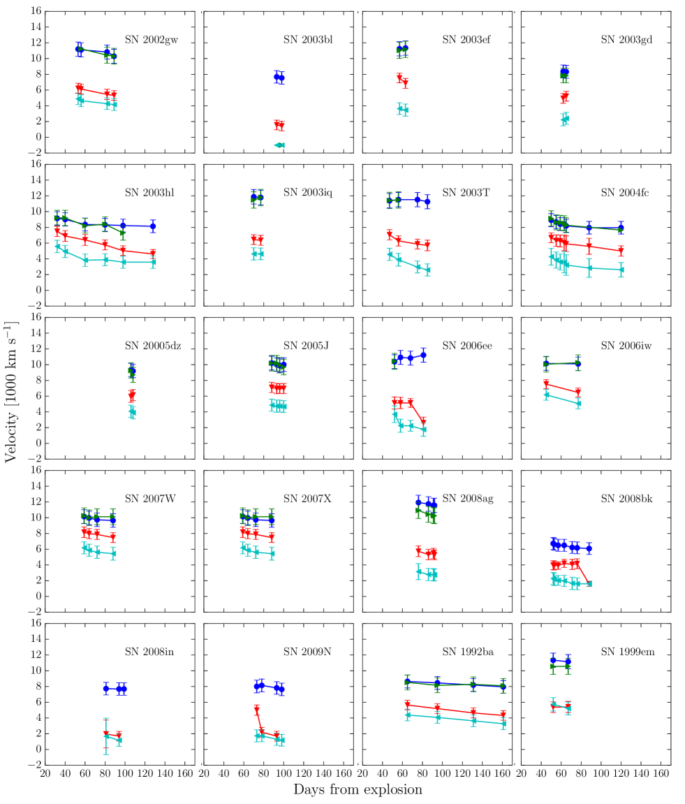
Figure 25.— Velocity evolution of Cachito in the plateau phase compared with the Balmer lines. In blue: HV of H_α, in green: HV of H_β, in red: the H_α velocity and in cyan the H_β velocity.

In addition to the 70 SNe where Cachito can be identified either with Si II or HV features of H I, we find six SNe II that display Cachito at certain epochs, however its exact properties do not align with the above interpretations (because of differences in shape and/or velocity). These are SN 2003bl, SN 2005an, SN 2007U, SN 2008br, SN 2002gd and SN 2004fb. In summary 59% of the full SNe sample show Cachito at some epoch, while 41% never show this feature. Soon after shock-break out all SNe II have extremely high temperature ejecta. Therefore, if we were able to obtain spectral sequences shortly after explosion, the Si II feature would always be observed. However, observationally this is not the case as there are many SNe II within our sample without Si II detections. This is simply an observational bias, due to the lack of data at very early times. Nevertheless, for SNe II that stay hotter for longer the probability of detecting Si II becomes larger. We therefore speculate that SNe II that have detected Si II at early times have larger radii, which leads to a slower cooling of the ejecta and hence facilitates Si II detection. Interestingly, when we split the sample into those SNe II that do and do not display the Si II line, those where the line is detected are found to have lower $a/e$ values, with only a 4% chance that the two populations are drawn from the same underlying distribution. This is also consistent with the previous finding that those SNe II with evident He I detections at around 20 days post explosion are also found to have lower $a/e$ values, suggesting that the value of $a/e$ is related to ejecta temperature evolution.
In the case of those SNe II displaying Cachito consistent with HV features, these are most likely produced by the interaction of the SN ejecta with the RSG wind, where the exact shape and persistence of Cachito is related to the wind density Chugai et al. (2007). In Figure 26 one can observe the significant diversity in the different detection of Cachito.

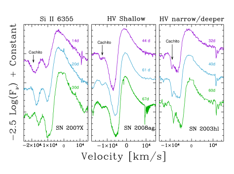
Figure 26.— Cachito’s shape according to its nature. On left panel: The Si II line in SN 2007X. In the middle panel: HV features of H I as a shallow absorption in SN 2008ag. On right panel: HV features of H I as narrow and deeper absorption component in SN 2003hl.

IX. Conclusions

In this paper we have presented optical spectra of 122 nearby SNe II observed between 1986 and 2009. A total of 888 spectra ranging between 3 and 363 days post explosion have been analyzed. The spectral matching technique was discussed as an alternative to non-detection constraints for estimating SN explosion epochs.
In order to quantify the spectral diversity we analyze the appearance of the photospheric lines and their time evolution in terms of the $a/e$ and H_α velocity at the $B$-band transition time plus 10 days (t_tran+10; see Gutiérrez et al. 2014 for more details), the magnitude at maximum (M_max), the plateau decline (s₂), and metallicity (M13 N2). We analyzed the velocity decline rate of H_β, the $a/e$ evolution, the expansion ejecta velocities and the pEWs for eleven features: H_α, H_β, He I/Na I D, Fe II $\lambda 4924$, Fe II $\lambda 5018$, Fe II $\lambda 5169$, Fe II blend, Sc II/Fe II, Sc II multiplet, Ba II, Sc II, and O I. We find a large range in velocities and pEWs, which may be related with a diversity in the explosion energy, radius of the progenitor, and metallicity. The evolution of line strengths was analyzed and compared to that of spectral models. SNe II displaying differences in spectral line evolution were also found to have other different spectral, photometric and environmental properties. Finally, we discuss the detection and origin of Cachito on the blue side of H_α.
The main results obtained with our analysis are summarized as follows:

• The line evolution indicates differences in temperatures and/or metallicity. Thus, SNe with slower temperature gradients show the appearance of the iron lines later, while SNe in environments with higher metallicities show them earlier. In fact, the Fe II line forest is present in faint SNe with low ejecta temperatures and/or in high metallicity environments. Comparing this result with the synthetic spectra, we find that indeed this feature is only present in higher metallicity (2 times solar) and lower explosion energy models, which is consistent with our observations.

• SNe II display a significant variety of expansion velocities, suggesting a large range in explosion energies.

• At early phases (before 25 days), SNe II with a weak H_α absorption component show He I $\lambda 5876$ and the Si II $\lambda 6355$ features. We speculate that this occurs because of higher temperatures at these epochs.

• Around 60% of our SNe II show the Cachito feature between 7 and 120 days since explosion. When Cachito is detected less than 30 days post explosion then it is identified with Si II. The epochs of early detection can thus inform us to the temperature evolution: SNe II with Si II detections at later epochs have higher temperatures, and this may be related to higher-radius progenitors. At later epochs, during the recombination phase, we suggest that Cachito is related to HV of hydrogen lines. Such HV features are most likely related to the interaction of the SN ejecta with the RSG wind.

All data analyzed in this work are available on http://csp.obs.carnegiescience.edu/, as well as the additional SNID templates (22 SNe), for the SNe II comparison.

Table 1SN II sample

	Host	Recession	Hubble	$E(B-V)_{\rm MW}$	Discovery	Discovery	Explosion	N of
SN	Galaxy	velocity (km s-1)	type	(mag)	date	Reference	Epoch	spectra	Campaign
1986L	NGC 1559	1305	SBcd	0.026	46711.1	IAUC 4260	46708.0n(3)	31	CTSS
1988A	NGC 4579	1517	SABb	0.036	47179.0	IAUC 4533	47177.2n(2)	5	CTSS
1990E	NGC 1035	1241	SAc	0.022	47937.7	IAUC 4965	47935.1n(3)	5	CTSS
1990K	NGC 0150	1584	SBbc	0.013	48037.3	IAUC 5022	48001.5n(6)	9	CTSS
1991al	2MASX J19422191–5506275	45751	?	0.054	48453.7	IAUC 5310	48442.5s(8)*	8	CT
1992af	ESO 340-G038	5541	S	0.046	48802.8	IAUC 5554	48798.8s(8)*	5	CT
1992am	MCG -01-04-039	143971	S	0.046	48829.8	IAUC 5570	48813.9s(6)*	2	CT
1992ba	NGC 2082	1185	SABc	0.051	48896.2	IAUC 5625	48884.9s(7)	10	CT
1993A	2MASX J07391822–6203095	87901	?	0.153	49004.6	IAUC 5693	48995.5n(9)	2	CT
1993K	NGC 2223	2724	SBbc	0.056	49075.5	IAUC 5733	49065.5n(9)	17	CT
1993S	2MASX J22522390-4018432	9903	S	0.014	49133.7	IAUC 5812	49130.8s(5)	4	CT
1999br	NGC 4900	960	SBc	0.021	51281.0	IAUC 7141	51276.7n(4)	8	SOIRS
1999ca	NGC 3120	2793	Sc	0.096	51296.0	IAUC 7158	51277.5s(7)*	4	SOIRS
1999cr	ESO 576-G034	60691	S/Irr	0.086	51249.7	IAUC 7210	51246.5s(4)*	5	SOIRS
1999eg	IC 1861	6708	SA0	0.104	51455.5	IAUC 7275	51449.5s(6)*	2	SOIRS
1999em	NGC 1637	717	SABc	0.036	51481.0	IAUC 7294	51476.5n(5)	12	SOIRS
2002ew	NEAT J205430.50-000822.0	8975	?	0.091	52510.8	IAUC 7964	52500.6n(10)	7	CATS
2002fa	NEAT J205221.51+020841.9	17988	?	0.088	52510.8	IAUC 7967	52502.5s(8)*	6	CATS
2002gd	NGC 7537	2676	SAbc	0.059	52552.7	IAUC 7986	52551.5s(4)*	12	CATS
2002gw	NGC 922	3084	SBcd	0.017	52560.7	IAUC 7995	52553.5s(8)*	11	CATS
2002hj	NPM1G +04.0097	7080	?	0.102	52568.0	IAUC 8006	52562.5n(7)	7	CATS
2002hx	PGC 023727	9293	SBb	0.048	52589.7	IAUC 8015	52582.5n(9)	9	CATS
2002ig	SDSS J013637.22+005524.9	231002	?	0.034	52576.7	IAUC 8020	52570.5s(5)*	5	CATS
210	MCG +00-03-054	15420	?	0.033	?3	?	52486.5s(6)*	6	CATS
2003B	NGC 1097	1272	SBb	0.024	52645.0	IAUC 8042	52613.5s(11)*	9	CATS
2003E	MCG -4-12-004	44701	Sbc	0.043	52645.0	IAUC 8044	52629.5s(8)*	8	CATS
2003T	UGC 4864	8373	SAab	0.028	52665.0	IAUC 8058	52654.5n(10)	6	CATS
2003bl	NGC 5374	43771	SBbc	0.024	52701.0	IAUC 8086	52696.5s(4)*	8	CATS
2003bn	2MASX J10023529-2110531	3828	?	0.057	52698.0	IAUC 8088	52694.5n(3)	12	CATS
2003ci	UGC 6212	9111	Sb	0.053	52720.0	IAUC 8097	52711.5n(8)	7	CATS
2003cn	IC 849	54331	SABcd	0.019	52728.0	IAUC 8101	52717.5s(4)*	5	CATS
2003cx	NEAT J135706.53-170220.0	11100	?	0.083	52730.0	IAUC 8105	52725.5s(5)*	6	CATS
2003dq	MAPS-NGP O4320786358	13800	?	0.016	52739.7	IAUC 8117	52731.5n(8)	3	CATS
2003ef	NGC 4708	44401	SAab	0.041	52770.7	IAUC 8131	52757.5s(9)*	6	CATS
2003eg	NGC 4727	43881	SABbc	0.046	52776.7	IAUC 8134	52764.5s(5)*	5	CATS
2003ej	UGC 7820	5094	SABcd	0.017	52779.7	IAUC 8134	52775.5n(5)	3	CATS
2003fb	UGC 11522	52621	Sbc	0.162	52796.0	IAUC 8143	52772.5s(10)*	4	CATS
2003gd	M74	657	SAc	0.062	52803.2	IAUC 8150	52755.5s(9)*	3	CATS
2003hd	MCG -04-05-010	11850	Sb	0.011	52861.0	IAUC 8179	52855.9s(5)*	9	CATS
2003hg	NGC 7771	4281	SBa	0.065	52870.0	IAUC 8184	52865.5n(5)	5	CATS
2003hk	NGC 1085	6795	SAbc	0.033	52871.6	CBET 41	52866.8s(4)*	4	CATS
2003hl	NGC 772	2475	SAb	0.064	52872.0	IAUC 8184	52868.5n(5)	6	CATS
2003hn	NGC 1448	1170	SAcd	0.013	52877.2	IAUC 8186	52866.5n(10)	9	CATS
2003ho	ESO 235-G58	4314	SBcd	0.034	52851.9	IAUC 8186	52848.5s(7)*	5	CATS
2003ib	MCG -04-48-15	7446	Sb	0.043	52898.7	IAUC 8201	52891.5n(8)	5	CATS
2003ip	UGC 327	5403	Sbc	0.058	52913.7	IAUC 8214	52896.5s(4)	4	CATS
2003iq	NGC 772	2475	SAb	0.064	52921.5	CBET 48	52919.5n(2)	5	CATS
2004dy	IC 5090	9352	Sa	0.045	53242.5	IAUC 8395	53240.5n(2)	3	CSP
2004ej	NGC 3095	2723	SBc	0.061	53258.5	CBET 78	53223.9s(9)*	9	CSP
2004er	MCG -01-7-24	4411	SAc	0.023	53274.0	CBET 93	53271.8n(2)	10	CSP
2004fb	ESO 340-G7	6100	S	0.056	53286.2	IAUC 8420	53258.6s(7)*	4	CSP
2004fc	NGC 701	1831	SBc	0.023	53295.2	IAUC 8422	53293.5n(1)	10	CSP
2004fx	MCG -02-14-3	2673	SBc	0.090	53307.0	IAUC 8431	53303.5n(4)	10	CSP
2005J	NGC 4012	4183	Sb	0.025	53387.0	IAUC 8467	53379.8s(7)*	11	CSP
2005K	NGC 2923	8204	?	0.035	53386.0	IAUC 8468	53369.8s(8)	2	CSP
2005Z	NGC 3363	5766	S	0.025	53402.0	IAUC 8476	53396.7n(6)	9	CSP
2005af	NGC 4945	563	SBcd	0.156	53409.7	IAUC 8482	53320.8s(17)*	9	CSP
2005an	ESO 506-G11	3206	S0	0.083	53432.7	CBET 113	53431.8s(6)*	7	CSP
2005dk	IC 4882	4708	SBb	0.043	53604.0	IAUC 8586	53601.5s(6)*	7	CSP
2005dn	NGC 6861	2829	SA0	0.048	53609.5	IAUC 8589	53602.6s(6)*	8	CSP
2005dt	MCG -03-59-6	7695	SBb	0.025	53614.7	CBET 213	53605.6n(9)	1	CSP
2005dw	MCG -05-52-49	5269	Sab	0.020	53612.7	CBET 219	53603.6n(9)	3	CSP
2005dx	MCG -03-11-9	8012	S	0.021	53623.0	CBET 220	53611.8s(7)*	1	CSP
2005dz	UGC 12717	5696	Scd	0.072	53623.7	CBET 222	53619.5n(4)	7	CSP
2005es	MCG +01-59-79	11287	S	0.076	53643.7	IAUC 8608	53638.7n(5)	1	CSP
2005gz	MCG -01-53-022	8518	SBbc	0.06	53654.7	IAUC 8616	53650.2n(5)	1	CSP
2005lw	IC 672	7710	?	0.043	53719.0	CBET 318	53716.8s(10)	14	CSP
2005me	ESO 244-31	6726	SAc	0.022	53728.2	CBET 333	53717.9s(10)*	1	CSP
2006Y	anon	100742	?	0.115	53770.0	IAUC 8668	53766.5n(4)	13	CSP
2006ai	ESO 005-G009	45711	SBcd	0.113	53784.0	CBET 406	53781.6s(5)	12	CSP
2006bc	NGC 2397	1363	SABb	0.181	53819.1	CBET 446	53815.5n(4)	3	CSP
2006be	IC 4582	2145	S	0.026	53819.0	CBET 449	53802.8s(9)*	4	CSP
2006bl	MCG +02-40-9	9708	?	0.045	53829.5	CBET 597	53822.7s(10)*	3	CSP
2006ee	NGC 774	4620	S0	0.054	53966.0	cbet 597	53961.9n(4)	13	CSP
2006it	NGC 6956	4650	SBb	0.087	54009.5	CBET 660	54006.5n(3)	6	CSP
2006iw	2MASX J23211915+0015329	9226	?	0.044	54011.5	CBET 663	54010.7n(1)	5	CSP
2006ms	NGC 6935	4543	SAa	0.031	54046.2	CBET 725	54028.5s(6)**	4	CSP
2006qr	MCG -02-22-023	4350	SABbc	0.040	54070.0	CBET 766	54062.8n(7)	8	CSP
2007P	ESO 566-G36	12224	Sa	0.036	54124.0	CBET 819	54118.7n(5)	6	CSP
2007U	ESO 552-65	7791	S	0.046	54136.5	CBET 835	54133.6s(6)*	7	CSP
2007W	NGC 5105	2902	SBc	0.045	54146.5	CBET 844	54130.8s(7)*	7	CSP
2007X	ESO 385-G32	2837	SABc	0.060	54146.5	CBET 844	54143.5s(5)	12	CSP
2007Z	PGC 016993	5277	Sbc	0.525	54148.7	CBET 847	54135.6s(5)	2	CSP
2007aa	NGC 4030	1465	SAbc	0.023	54149.7	CBET 848	54126.7s(8)*	11	CSP
2007ab	MCG -01-43-2	7056	SBbc	0.235	54150.7	CBET 851	54123.9s(10)	5	CSP
2007av	NGC 3279	1394	Scd	0.032	54180.2	CBET 901	54173.8s(5)*	4	CSP
2007bf	UGC 09121	5327	Sbc	0.018	54285.0	CBET 919	54191.5n(7)	4	CSP
2007hm	SDSS J205755.65-072324.9	7540	?	0.059	54343.7	CBET 1050	54336.6s(6)*	7	CSP
2007il	IC 1704	6454	S	0.042	54354.0	CBET 1062	54349.8n(4)	12	CSP
2007it	NGC 5530	1193	SAc	0.103	54357.5	CBET 1065	54348.5n(1)	11	CSP
2007ld	anon	74991	?	0.081	54379.5	CBET 1098	54376.5s(8)*	7	CSP
2007oc	NGC 7418	1450	SABcd	0.014	54396.5	CBET 1114	54388.5n(3)	17	CSP
2007od	UGC 12846	1734	Sm	0.032	54407.2	CBET 1116	54400.6s(5)*	14	CSP
2007sq	MCG -03-23-5	4579	SAbc	0.183	54443.0	CBET 1170	54422.8s(6)*	7	CSP
2008F	MCG -01-8-15	5506	SBa	0.044	54477.5	CBET 1207	54469.6s(6)*	2	CSP
2008H	ESO 499- G 005	4287	SAc	0.057	54481.0	CBET 1210	54432.8s(8)	1	CSP
2008K	ESO 504-G5	7997	Sb	0.035	54481.0	CBET 1211	54475.5s(6)*	12	CSP
2008M	ESO 121-26	2267	SBc	0.040	54480.7	CBET 1214	54471.7n(9)	12	CSP
2008W	MCG -03-22-7	5757	Sc	0.086	54502.7	CBET 1238	54483.8s(8)*	10	CSP
2008ag	IC 4729	4439	SABbc	0.074	54499.5	CBET 1252	54477.9s(8)*	18	CSP
2008aw	NGC 4939	3110	SAbc	0.036	54528.0	CBET 1279	54517.8n(10)	12	CSP
2008bh	NGC 2642	4345	SBbc	0.020	54549.0	CBET 1311	54543.5n(5)	6	CSP
2008bk	NGC 7793	227	SAd	0.017	54550.7	CBET 1315	54540.9s(8)*	26	CSP
2008bm	CGCG 071-101	9563	Sc	0.023	54554.7	CBET 1320	54522.8s(6)	4	CSP
2008bp	NGC 3095	2723	SBc	0.061	54558.7	CBET 1326	54551.7n(6)	5	CSP
2008br	IC 2522	3019	SAcd	0.083	54564.2	CBET 1332	54555.7n(9)	4	CSP
2008bu	ESO 586-G2	6630	S	0.376	54574.0	CBET 1341	54566.8s(7)	5	CSP
2008ga	LCSB L0250N	4639	?	0.582	54734.0	CBET 1526	54711.5s(7)	3	CSP
2008gi	CGCG 415-004	7328	Sc	0.060	54752.0	CBET 1539	54742.7n(9)	6	CSP
2008gr	IC 1579	6831	SBbc	0.012	54768.7	CBET 1557	54769.6s(6)*	5	CSP
2008hg	IC 1720	5684	Sbc	0.016	54785.5	CBET 1571	54779.8n(5)	6	CSP
2008ho	NGC 922	3082	SBcd	0.017	54796.5	CBET 1587	54792.7n(5)	3	CSP
2008if	MCG -01-24-10	3440	Sb	0.029	54812.7	CBET 1619	54807.8n(5)	20	CSP
2008il	ESO 355-G4	6276	SBb	0.015	54827.7	CBET 1634	54825.6n(3)	3	CSP
2008in	NGC 4303	1566	SABbc	0.020	54827.2	CBET 1636	54825.4n(2)*	13	CSP
2009N	NGC 4487	1034	SABcd	0.019	54856.3	CBET 1670	54846.8s(5)	13	CSP
2009W	SDSS J162346.79+114423	5100	?	0.065	54865.0	CBET 1683	54816.9s(9)	1	CSP
2009aj	ESO 221- G 018	2883	Sa	0.130	54887.0	CBET 1704	54880.5n(7)	12	CSP
2009ao	NGC 2939	3339	Sbc	0.034	54895.0	CBET 1711	54890.7n(4)	7	CSP
2009au	ESO 443-21	2819	Scd	0.081	54902.0	CBET 1719	54897.5n(4)	10	CSP
2009bu	NGC 7408	3494	SBc	0.022	54916.2	CBET 1740	54901.9s(8)*	6	CSP
2009bz	UGC 9814	3231	Sdm	0.035	54920.0	CBET 1748	54915.8n(4)	5	CSP

• ¹ Measured using our own spectra.
  ² Taken from the Asiago supernova catalog: http://graspa.oapd.inaf.it/ (Barbon et al., 1999).
  ³ The CATS survey performed the follow up of SN 210, which was discovered by the SN Factory Wood-Vasey et al. (2004) and was never reported to the International Astronomical Union (IAU) to provide an official designation.
  ^s Explosion epoch estimation through spectral matching.
  ⁿ Explosion epoch estimation from SN non-detection.
  ^∗ Cases where explosion epochs have changed between Anderson et al. (2014b) and the current work.
  Observing campaigns: CTSS=Cerro Tololo Supernova Survey; CT=Calán/Tololo Supernova Program; SOIRS=Supernova Optical and Infrared Survey; CATS=Carnegie Type II Supernova Survey; CSP=Carnegie Supernova Project.

• In the first column the SN name, followed by its host galaxy are listed. In column 3 we list the host galaxy heliocentric recession velocity. These are taken from the Nasa Extragalactic Database (NED: http://ned.ipac.caltech.edu/) unless indicated by a superscript (sources in table notes). In columns 4 and 5 we list the host galaxy morphological Hubble types (from NED) and the reddening due to dust in our Galaxy (Schlafly & Finkbeiner, 2011) taken from NED. In column 6, 7 and 8 we list the discovery date, their reference and the explosion epochs. The number of spectra and the the observing campaign from which each SN was taken are given in column 9 and 10, and acronyms are listed in the table notes.
  

Table 2Reference SNe II

SN	Explosion date	V-Maximum date	Days from Explosion to V-maximum	Reference
1999em	2451475.6 (5)	2451485.5	5	Leonard et al. 2002b
1999gi	2451518.3 (3)	2451530.0	12	Leonard et al. 2002a
2004et	2453270.5 (3)	2453286.6	16	Li et al. 2005; Sahu et al. 2006
2005cs	2453547.6 (1)	2453553.6	6	Pastorello et al. 2006
2006bp	2453833.4 (1)	2453842.0	9	Dessart et al. 2008
1988A	2447177.2 (2)	$\cdots$	$\cdots$	This work
1990E	2447935.1 (3)	$\cdots$	$\cdots$	This work
1999br	2451276.7 (4)	$\cdots$	$\cdots$	This work
2003bn	2452694.5 (3)	$\cdots$	$\cdots$	This work
2003iq	2452919.5 (2)	$\cdots$	$\cdots$	This work
2004er	2453271.8 (2)	$\cdots$	$\cdots$	This work
2004fc	2453293.5 (1)	$\cdots$	$\cdots$	This work
2004fx	2453303.5 (4)	$\cdots$	$\cdots$	This work
2005dz	2453619.5 (4)	$\cdots$	$\cdots$	This work
2006bc	2453815.5 (4)	$\cdots$	$\cdots$	This work
2006ee	2453961.9 (4)	$\cdots$	$\cdots$	This work
2006it	2454006.5 (3)	$\cdots$	$\cdots$	This work
2006iw	2454010.7 (1)	$\cdots$	$\cdots$	This work
2006Y	2453766.5 (4)	$\cdots$	$\cdots$	This work
2007il	2454349.8 (4)	$\cdots$	$\cdots$	This work
2007it	2454348.5 (1)	$\cdots$	$\cdots$	This work
2007oc	2454388.5 (3)	$\cdots$	$\cdots$	This work
2008il	2454825.6 (3)	$\cdots$	$\cdots$	This work
2008in	2454825.4 (2)	$\cdots$	$\cdots$	This work
2009ao	2454890.7 (4)	$\cdots$	$\cdots$	This work
2009au	2454897.5 (4)	$\cdots$	$\cdots$	This work
2009bz	2454915.8 (4)	$\cdots$	$\cdots$	This work

• Columns: (1) SN name; (2) Julian date of the explosion epoch; (3) Julian date of the $V$-band maximum; (4) Days from Explosion to $V-$band maximum; (5) References.
  The first five SNe are included in SNID and are used as templates in this work. Their respective references are presented in the column 4. The rest of SNe showed after the line are taken from this work as new SNID templates.

Table 3Spectral features used to the statistical analysis in the photospheric and nebular phases

Feature name	Rest wavelength⋆ [Å]	Blue-ward limit range♣ [Å]	Red-ward limit range♣ [Å]
Hα	6563	6000 - 6300	6900 - 7100
Hβ	4861	4400 - 4700	4800 - 4900
Fe II	4924	4800 - 4900	4900 - 4950
Fe II	5018	4900 - 4500	5000 - 5050
Fe II	5169	5000 - 5050	5100 - 5300
Na I	5893	5500 - 6000	5800 - 6000
Sc II	5531	5400 - 5450	5500- 5550
Sc II/Fe II	5663	5500 - 5550	5600 - 5700
Ba II	6142	6000 - 6050	6100 - 6150
Sc II	6247	6150 - 6170	6250 - 6270
O I	7774	7630 - 7650	7750 - 7780

• ^⋆ The rest wavelengths are weighted averages of the strongest spectral lines that give rise to each absorption feature.
  ^♣ These limits are necessary in order to account for variations in spectral feature width and expansion velocity among SNe.

Table 4KS-Test values

Feature name	$v$(Hα)	$a/e$	Mmax	$s_{2}$	M13N2	Epoch [days]
Fe II line forest	5.19	9.80	2.17	$3.73\times 10^{-4}$	4.38	0 - 100
Hγ blended	29.75	58.33	31.21	55.32	16.10	23 - 27
He I 5876	18.62	1.91	30.94	25.73	46.18	18 - 22
Ca II IR triplet	87.73	91.97	94.47	53.30	98.82	18 - 22
Fe II 4924	2.82	16.84	1.09	4.80	99.40	28 - 32
Fe II 5018	15.68	90.80	99.02	68.84	61.53	18 - 22
Fe II 5169	60.76	35.15	74.88	50.83	20.30	13 - 17
Fe II multiplet	21.38	26.75	1.00	0.25	99.28	33 - 37
Sc II/Fe II 5531	75.60	89.60	30.34	45.20	1.84	38 - 42
Sc II multiplet 5663	63.54	63.54	30.34	80.10	0.79	38 - 42
Ba II 6142	45.75	83.58	1.90	57.43	1.29	38 - 42
Sc II 6247	45.76	83.58	1.89	57.42	0.52	38 - 42

• Percentage obtained using a KS Test to verify if two distributions (with and without each line ) are drawn from the same parent population as a function of $v$(H_α), $a/e$, M_max, $s_{2}$, and M13N2 in an particular epoch. This epoch is shown in the last column of the table.

Table 5Model properties

Model	Z	Mfinal	R∗	Ekin
	[Z⊙]	[M⊙]	[R⊙]	[B]
m15z2m3	0.1	14.92	524	1.35
m15z8m3	0.4	14.76	611	1.27
m15z8m3	1.0	14.09	768	1.27
m15z4m2	2.0	12.60	804	1.24
m15mlt1	1.0	14.01	1107	1.24
m15mlt3	1.0	14.08	501	1.34
m12mlt3	1.0	10.50	500	0.25

• Summary of model properties used in this work.
  Columns: (1) Model name; (2) Metallicity; (3) Final progenitor mass; (4) Progenitor radius; (5) Kinetic energy

Table A1Spectroscopic observations information

UT Date	JD	Phase	Tel.	Inst.	Wavelength	Resol.	Exp.	Air-
		(days)			Range (AA)	(AA)	(s)	mass
(1)	(2)	(3)	(4)	(5)	(6)	(7)	(8)	(9)
SN 1986L
1986-10-09	2446712.50	4	$\cdots$	$\cdots$	3681-7728	$\cdots$	1000	1.21
1986-10-11	2446714.50	6	$\cdots$	$\cdots$	3730-7168	$\cdots$	1556	1.20
1986-10-12	2446715.50	7	$\cdots$	$\cdots$	3800-7322	$\cdots$	2000	1.21
1986-10-13	2446716.50	8	$\cdots$	$\cdots$	3681-4988	$\cdots$	1352	1.21⋆
1986-10-14	2446717.50	9	$\cdots$	$\cdots$	3681-4988	$\cdots$	2500	1.19⋆
1986-10-15	2446718.50	10	$\cdots$	$\cdots$	3681-4988	$\cdots$	2500	1.18⋆
1986-10-20	2446723.50	15	$\cdots$	$\cdots$	3720-5031	$\cdots$	3000	1.24⋆
1986-10-26	2446729.50	21	$\cdots$	$\cdots$	3830-7330	$\cdots$	2000	1.20
1986-10-28	2446731.50	23	$\cdots$	$\cdots$	3596-5125	$\cdots$	2000	1.37
1986-10-28	2446731.50	23	$\cdots$	$\cdots$	3590-5130	$\cdots$	$\cdots$	1.37
1986-10-29	2446732.50	24	$\cdots$	$\cdots$	3675-5240	$\cdots$	1200	1.23
1986-11-01	2446735.50	27	$\cdots$	$\cdots$	3270-7205	$\cdots$	1800	1.21
1986-11-02	2446736.50	28	$\cdots$	$\cdots$	3270-7205	$\cdots$	1200	1.2
1986-11-03	2446737.50	29	$\cdots$	$\cdots$	3847-7357	$\cdots$	2000	1.22
1986-11-03	2446737.50	29	$\cdots$	$\cdots$	3270-7205	$\cdots$	1200	1.21
1986-11-04	2446738.50	30	$\cdots$	$\cdots$	4166-7701	$\cdots$	1800	1.22
1986-11-04	2446738.50	30	$\cdots$	$\cdots$	3270-7205	$\cdots$	1200	1.20
1986-11-05	2446739.50	31	$\cdots$	$\cdots$	3270-7205	$\cdots$	1200	1.20
1986-11-06	2446740.50	32	$\cdots$	$\cdots$	3270-7205	$\cdots$	1200	1.21
1986-11-07	2446741.50	33	$\cdots$	$\cdots$	3270-7205	$\cdots$	1200	1.21
1986-11-10	2446744.50	36	$\cdots$	$\cdots$	4166-7701	$\cdots$	1800	1.23
1986-11-11	2446745.50	37	$\cdots$	$\cdots$	3830-7285	$\cdots$	1000	1.19
1986-11-14	2446748.50	40	$\cdots$	$\cdots$	3561-6446	$\cdots$	$\cdots$	1.20
1986-11-16	2446750.50	42	$\cdots$	$\cdots$	3561-6446	$\cdots$	$\cdots$	1.18
1986-11-25	2446759.50	51	$\cdots$	$\cdots$	3450-6950	$\cdots$	2000	1.20⋆
1986-12-09	2446773.50	65	$\cdots$	$\cdots$	3680-6670	$\cdots$	1000	1.44
1986-12-10	2446774.50	66	$\cdots$	$\cdots$	3769-7329	$\cdots$	2262	$\cdots$
1986-12-23	2446787.50	79	$\cdots$	$\cdots$	3991-7548	$\cdots$	2394	$\cdots$
1987-01-01	2446796.50	88	$\cdots$	$\cdots$	3776-7578	$\cdots$	2545	$\cdots$
1987-01-23	2446818.50	110	$\cdots$	$\cdots$	3450-6950	$\cdots$	3000	1.20
1987-01-30	2446825.50	117	$\cdots$	$\cdots$	5601-7998	$\cdots$	$\cdots$	1.24
SN 1988A
1988-01-28	2447188.50	11	$\cdots$	$\cdots$	3047-7731	$\cdots$	600	1.37
1988-01-29	2447189.50	12	$\cdots$	$\cdots$	3034-7778	$\cdots$	600	1.35
1988-02-02	2447193.50	16	$\cdots$	$\cdots$	5786-10284	$\cdots$	600	1.34
1988-02-03	2447194.50	17	$\cdots$	$\cdots$	2914-7389	$\cdots$	600	1.34
1988-03-06	2447226.50	49	$\cdots$	$\cdots$	7699-10964	$\cdots$	600	1.48
SN 1990E
1990-02-23	2447945.50	10	$\cdots$	$\cdots$	3172-7910	$\cdots$	600	1.37
1990-03-04	2447954.50	19	$\cdots$	$\cdots$	3147-6412	$\cdots$	600	1.35
1990-03-04	2447954.50	19	$\cdots$	$\cdots$	3147-9083	$\cdots$	600	1.34
1990-03-19	2447969.50	34	$\cdots$	$\cdots$	5794-9082	$\cdots$	600	5.52
1990-07-03	2448075.50	140	$\cdots$	$\cdots$	2979-7726	$\cdots$	600	1.48
SN 1990K
1990-05-31	2448042.50	41	$\cdots$	$\cdots$	3177-6489	$\cdots$	240	1.23
1990-05-31	2448042.50	41	$\cdots$	$\cdots$	6180-9553	$\cdots$	360	1.38
1990-06-07	2448049.50	48	$\cdots$	$\cdots$	2980-7729	$\cdots$	900	1.31
1990-06-08	2448050.50	49	$\cdots$	$\cdots$	6078-10597	$\cdots$	900	1.23
1990-06-12	2448054.50	53	$\cdots$	$\cdots$	2982-7731	$\cdots$	900	1.15
1990-06-19	2448061.50	60	$\cdots$	$\cdots$	5933-10440	$\cdots$	600	1.33
1990-07-03	2448075.50	74	$\cdots$	$\cdots$	2980-7726	$\cdots$	1200	1.20
1990-08-13	2448116.50	115	$\cdots$	$\cdots$	2994-7733	$\cdots$	1800	1.01
1990-08-17	2448120.50	119	$\cdots$	$\cdots$	2982-7737	$\cdots$	1800	1.03
SN 1991al
1991-08-05	2448473.50	31	$\cdots$	$\cdots$	3595-9899	$\cdots$	$\cdots$	$\cdots$
1991-08-06	2448474.50	32	$\cdots$	$\cdots$	3545-6794	$\cdots$	$\cdots$	$\cdots$
1991-08-10	2448478.50	36	$\cdots$	$\cdots$	3545-9793	$\cdots$	$\cdots$	$\cdots$
1991-08-13	2448481.50	39	$\cdots$	$\cdots$	4432-7052	$\cdots$	$\cdots$	$\cdots$
1991-09-02	2448501.67	59	$\cdots$	$\cdots$	2961-7621	$\cdots$	3600	1.24
1991-09-14	2448513.68	71	$\cdots$	$\cdots$	3218-7417	$\cdots$	2x600	1.40
1991-10-10	2448538.61	97	$\cdots$	$\cdots$	2957-7612	$\cdots$	1800	1.41
1991-11-07	2448567.54	125	$\cdots$	$\cdots$	3157-7384	$\cdots$	600	1.45
SN 1992af
1992-07-09	2448812.87	14	$\cdots$	$\cdots$	4666-7037	$\cdots$	1800	1.25
1992-07-10	2448813.81	15	$\cdots$	$\cdots$	4667-7038	$\cdots$	1200	1.07
1992-07-29	2448832.76	34	$\cdots$	$\cdots$	3194-7364	$\cdots$	900	1.08
1992-10-01	2448896.59	98	$\cdots$	$\cdots$	3149-7360	$\cdots$	3x1200	1.08
1992-10-31	2448926.55	128	$\cdots$	$\cdots$	3152-7334	$\cdots$	3x1800	1.21
SN 1992am
1992-07-29	2448832.89	19	$\cdots$	$\cdots$	3106-7161	$\cdots$	900	1.10
1992-10-01	2448896.78	84	$\cdots$	$\cdots$	3061-7156	$\cdots$	3X900	1.16
SN 1992ba
1992-10-01	2448896.85	12	$\cdots$	$\cdots$	3196-7470	$\cdots$	4X180	1.23
1992-10-01	2448896.90	12	$\cdots$	$\cdots$	6159-10112	$\cdots$	120	1.20
1992-10-05	2448900.88	16	$\cdots$	$\cdots$	5968-10447	$\cdots$	150	1.20
1992-10-05	2448900.82	16	$\cdots$	$\cdots$	3119-7367	$\cdots$	4X900	1.25
1992-10-27	2448922.81	38	$\cdots$	$\cdots$	2944-7658	$\cdots$	2X1200	1.21
1992-11-23	2448949.80	65	$\cdots$	$\cdots$	3182-7425	$\cdots$	500	1.22
1992-12-18	2448974.83	95	$\cdots$	$\cdots$	3213-7468	$\cdots$	2X90	1.45
1993-01-28	2449015.69	131	$\cdots$	$\cdots$	3683-6977	$\cdots$	600	1.34
1993-02-27	2449045.66	161	$\cdots$	$\cdots$	3082-8918	$\cdots$	2X2700	1.67
1993-03-21	2449067.54	183	$\cdots$	$\cdots$	5806-9125	$\cdots$	4X480	1.34
SN 1993A
1993-01-28	2449015.72	20	$\cdots$	$\cdots$	3591-6803	$\cdots$	1200	1.22
1993-04-21	2449098.60	103	$\cdots$	$\cdots$	3132-7240	$\cdots$	2X900	1.56
SN 1993K
1993-04-01	2449078.50	13	$\cdots$	$\cdots$	3171-7610	$\cdots$	900	1.05
1993-04-21	2449098.55	33	$\cdots$	$\cdots$	3180-7386	$\cdots$	3x600	1.75
1993-04-28	2449105.50	40	$\cdots$	$\cdots$	3665-9759	$\cdots$	2x1200	1.31
1993-05-16	2449123.47	58	$\cdots$	$\cdots$	3657-9741	$\cdots$	2x300	1.61
1993-05-17	2449124.47	59	$\cdots$	$\cdots$	6001-9743	$\cdots$	$\cdots$	$\cdots$
1993-05-17	2449124.47	59	$\cdots$	$\cdots$	7053-6728	$\cdots$	$\cdots$	$\cdots$
1993-11-17	2449308.83	243	$\cdots$	$\cdots$	5789-8357	$\cdots$	$\cdots$	1.00
1993-11-18	2449309.78	244	$\cdots$	$\cdots$	4453-8357	$\cdots$	$\cdots$	1.02
1993-11-18	2449309.82	244	$\cdots$	$\cdots$	4453-7053	$\cdots$	$\cdots$	1.00
1993-11-18	2449309.50	244	$\cdots$	$\cdots$	4453-7053	$\cdots$	$\cdots$	1.02
1993-12-15	2449336.78	271	$\cdots$	$\cdots$	3660-6825	$\cdots$	2x1800	1.02
1994-01-14	2449366.65	301	$\cdots$	$\cdots$	6355-10282	$\cdots$	1200	1.10
1994-01-14	2449366.66	301	$\cdots$	$\cdots$	6355-10282	$\cdots$	1800	1.15
1994-01-14	2449366.60	301	$\cdots$	$\cdots$	3696-6817	$\cdots$	1800	1.01
1994-01-14	2449366.62	301	$\cdots$	$\cdots$	3657-6827	$\cdots$	1500	1.04
1994-02-10	2449393.70	328	$\cdots$	$\cdots$	5802-8370	$\cdots$	$\cdots$	1.29
1994-03-17	2449428.58	363	$\cdots$	$\cdots$	4181-7506	$\cdots$	3600	1.16
SN 1993S
1993-06-26	2449164.76	34	$\cdots$	$\cdots$	2903-7478	$\cdots$	2x1800	1.28
1993-06-28	2449166.50	36	$\cdots$	$\cdots$	3872-9339	$\cdots$	$\cdots$	$\cdots$
1993-07-23	2449191.92	61	$\cdots$	$\cdots$	3111-7448	$\cdots$	1800	1.21
1993-08-24	2449223.76	93	$\cdots$	$\cdots$	3574-9523	$\cdots$	2x1800	1.02
SN 1999br
1999-04-23	2451291.50	15	$\cdots$	$\cdots$	3463-9271	$\cdots$	3x600	1.30
1999-04-26	2451294.50	18	$\cdots$	$\cdots$	2990-11961	$\cdots$	900	1.19
1999-04-29	2451297.50	21	$\cdots$	$\cdots$	2990-11961	$\cdots$	600	1.20
1999-05-03	2451301.50	25	$\cdots$	$\cdots$	2990-11961	$\cdots$	600	1.18
1999-05-11	2451309.50	33	$\cdots$	$\cdots$	2990-11961	$\cdots$	900	1.47
1999-05-19	2451317.50	41	$\cdots$	$\cdots$	2990-11961	$\cdots$	400	1.37
1999-05-21	2451320.02	43	$\cdots$	$\cdots$	3339-10249	$\cdots$	2x1800	1.24
1999-07-21	2451380.45	104	$\cdots$	$\cdots$	3113-8757	$\cdots$	2400	1.29
SN 1999ca
1999-05-06	2451303.50	26	$\cdots$	$\cdots$	10603-14225	$\cdots$	4x303	1.20⋆
1999-05-07	2451304.50	27	$\cdots$	$\cdots$	3170-10005	$\cdots$	600	1.04
1999-05-11	2451305.50	31	$\cdots$	$\cdots$	3338-10080	$\cdots$	900	1.10
1999-05-19	2451309.50	39	$\cdots$	$\cdots$	3170-10006	$\cdots$	400	1.11
SN 1999cr
1999-03-20	2451257.50	11	DUP	$\cdots$	3528-9086	$\cdots$	4x900	1.03
1999-03-30	2451267.50	21	$\cdots$	$\cdots$	3430-8821	$\cdots$	600	1.02
1999-04-23	2451291.50	45	DUP	$\cdots$	3406-9116	$\cdots$	2x1200	1.30
1999-05-03	2451301.50	55	$\cdots$	$\cdots$	3136-9893	$\cdots$	600	1.04
1999-05-07	2451305.50	59	$\cdots$	$\cdots$	3136-9901	$\cdots$	600	1.02
SN 1999eg
1999-10-16	2451467.50	18	DUP	$\cdots$	3521-9038	$\cdots$	1200	1.74
1999-11-19	2451501.50	52	NTT	$\cdots$	4597-9879	$\cdots$	200	1.76
SN 1999em
1999-11-02	2451484.50	8	$\cdots$	$\cdots$	8978-12653	$\cdots$	3x200	1.59
1999-11-03	2451485.50	9	$\cdots$	$\cdots$	3292-10074	$\cdots$	200	1.40
1999-11-09	2451491.50	15	$\cdots$	$\cdots$	3292-10074	$\cdots$	150	1.32
1999-11-14	2451496.50	20	$\cdots$	$\cdots$	3292-10074	$\cdots$	150	1.23
1999-11-18	2451500.50	24	$\cdots$	$\cdots$	2992-26935	$\cdots$	3x200	1.27
1999-11-19	2451501.50	25	$\cdots$	$\cdots$	3292-10074	$\cdots$	150	1.23
1999-11-28	2451510.50	34	$\cdots$	$\cdots$	8978-26935	$\cdots$	2x200	1.18
1999-12-16	2451528.75	52	$\cdots$	$\cdots$	4907-9257	$\cdots$	2x900	1.23
1999-12-31	2451543.75	67	$\cdots$	$\cdots$	3092-7109	$\cdots$	2x450	1.22
2000-04-09	2451643.50	167	$\cdots$	$\cdots$	3292-10074	$\cdots$	300	2.42
SN 2002ew
2002-09-12	2452329.50	29	DUP	WF	3670-7080	$\cdots$	2x1800	1.43
2002-09-13	2452329.50	30	DUP	WF	3670-7080	$\cdots$	1800	1.33⋆
2002-09-28	2452545.50	45	CLA	LD	3496-8740	$\cdots$	600	1.38
2002-10-08	2452555.50	55	DUP	WF	3709-9060	$\cdots$	2x900	1.61
2002-10-15	2452562.50	62	CLA	LD	3496-8740	$\cdots$	600	1.41
2002-10-25	2452572.50	72	CLA	LD	3496-8740	$\cdots$	600	1.00
2002-10-29	2452576.50	76	CLA	LD	3496-8740	$\cdots$	600	1.79
SN 2002fa
2002-09-12	2452529.50	27	DUP	WF	3565-6875	$\cdots$	2x1800	1.17
2002-09-28	2452545.50	43	CLA	LD	3395-8489	$\cdots$	600	1.29
2002-10-08	2452555.50	53	DUP	WF	3603-8800	$\cdots$	5x900	1.21
2002-10-14	2452561.50	59	CLA	LD	3395-8489	$\cdots$	600	1.17
2002-10-25	2452572.50	70	CLA	LD	3395-8489	$\cdots$	900	1.00
2002-10-29	2452576.50	74	CLA	LD	3395-8489	$\cdots$	900	1.35
SN 2002gd
2002-10-08	2452555.50	4	DUP	WF	3786-9247	$\cdots$	2x300	1.89
2002-10-14	2452561.50	10	CLA	LD	3568-8920	$\cdots$	300	1.36
2002-10-25	2452572.50	21	CLA	LD	3568-8920	$\cdots$	300	1.00
2002-10-29	2452576.50	25	CLA	LD	3568-8920	$\cdots$	300	1.42
2002-10-30	2452577.50	26	DUP	WF	3786-9247	$\cdots$	450	1.30
2002-11-07	2452585.50	34	DUP	WF	3786-9247	$\cdots$	450	1.28
2002-11-10	2452588.50	37	CLA	LD	3568-8920	$\cdots$	180	2.00
2002-11-12	2452590.50	39	CLA	LD	3151-9247	$\cdots$	300	1.55
2002-11-28	2452606.50	55	CLA	LD	3151-9247	$\cdots$	300	1.24
2002-12-01	2452609.50	58	DUP	WF	3786-9247	$\cdots$	600	1.57
2002-12-27	2452635.50	84	DUP	WF	3746-7215	$\cdots$	3x600	1.86
2003-01-09	2452648.50	97	CLA	LD	3151-9247	$\cdots$	300	2.42
SN 2002gw
2002-10-25	2452572.50	19	CLA	LD	3563-8908	$\cdots$	300	1.00
2002-10-29	2452576.50	23	CLA	LD	3563-8908	$\cdots$	300	1.03
2002-10-30	2452577.50	24	DUP	WF	3781-9234	$\cdots$	450	1.04
2002-11-07	2452585.50	32	DUP	WF	3781-9234	$\cdots$	450	1.00
2002-11-10	2452588.50	35	CLA	LD	3563-8908	$\cdots$	200	1.26
2002-11-12	2452590.50	37	CLA	LD	3147-9234	$\cdots$	300	1.06
2002-11-28	2452606.50	53	CLA	LD	3147-9234	$\cdots$	300	1.03
2002-12-01	2452609.50	56	DUP	WF	3781-9234	$\cdots$	600	1.02
2002-12-27	2452635.50	82	DUP	WF	3741-7205	$\cdots$	3x600	1.53
2003-01-03	2452642.50	89	DUP	WF	3741-7205	$\cdots$	3x600	1.93
2003-01-10	2452649.50	96	CLA	LD	3147-9234	$\cdots$	300	1.51
SN 2002hj
2002-11-07	2452585.50	23	DUP	WF	3731-9114	$\cdots$	450	1.21
2002-11-10	2452588.50	26	CLA	LD	3516-8792	$\cdots$	200	1.59
2002-11-12	2452590.50	28	CLA	LD	3106-9114	$\cdots$	300	1.25
2002-11-28	2452606.50	44	CLA	LD	3180-9330	$\cdots$	300	1.22
2002-12-03	2452611.50	49	DUP	WF	3731-9114	$\cdots$	600	1.22
2002-12-27	2452635.50	73	DUP	WF	3692-7111	$\cdots$	3x600	1.51
2003-01-08	2452647.50	85	CLA	LD	3106-9114	$\cdots$	300	1.45
SN 2002hx
2002-11-28	2452606.50	24	CLA	LD	3084-9049	$\cdots$	300	1.22
2002-12-01	2452609.50	27	DUP	WF	3705-9049	$\cdots$	600	1.11
2002-12-27	2452635.50	53	DUP	WF	3666-7061	$\cdots$	3x600	1.07
2003-01-03	2452642.50	60	DUP	WF	3666-7061	$\cdots$	3x600	1.04
2003-01-08	2452647.50	65	CLA	LD	3084-9049	$\cdots$	300	1.12
2003-01-09	2452648.50	66	CLA	LD	3084-9049	$\cdots$	600	1.12
2003-01-27	2452666.50	84	DUP	WF	3705-9049	$\cdots$	1200	1.14
2003-02-03	2452673.50	91	DUP	WF	3705-9049	$\cdots$	900	1.06
2003-03-04	2452702.50	120	DUP	WF	3685-9044	$\cdots$	900	1.13
SN 2002ig
2002-11-10	2452588.50	18	CLA	LD	3345-8364	$\cdots$	200	1.17
2002-11-12	2452590.50	20	CLA	LD	2955-8671	$\cdots$	300	1.16
2002-11-28	2452606.50	36	CLA	LD	2955-8671	$\cdots$	450	1.18
2002-12-03	2452611.50	41	DUP	WF	3550-8671	$\cdots$	900	1.17
2002-12-27	2452635.50	65	DUP	WF	3513-6765	$\cdots$	4x900	1.46
SN 210
2002-09-28	2452588.50	59	CLA	LD	3424-8560	$\cdots$	450	1.21
2002-09-30	2452590.50	60	DUP	WF	3633-8874	$\cdots$	4x900	1.32
2002-10-08	2452606.50	69	DUP	WF	3633-8874	$\cdots$	4x900	1.37
2002-10-14	2452611.50	75	CLA	LD	3424-8560	$\cdots$	600	1.44
2002-10-25	2452635.50	86	CLA	LD	3424-8560	$\cdots$	900	1.00
2002-10-29	2452635.50	90	CLA	LD	3424-8560	$\cdots$	900	1.16
SN 2003B
2003-01-06	2452645.50	32	$\cdots$	$\cdots$	3684-8961	$\cdots$	$\cdots$	$\cdots$
2003-01-08	2452647.50	34	CLA	LD	3166-9290	$\cdots$	200	1.00
2003-01-09	2452648.50	35	CLA	LD	3166-9290	$\cdots$	200	1.13
2003-01-10	2452649.50	36	CLA	LD	3166-9290	$\cdots$	200	1.45
2003-02-03	2452673.50	60	DUP	WF	3783-9285	$\cdots$	600	2.17
2003-03-02	2452700.50	87	DUP	WF	3803-9290	$\cdots$	600	1.61
2003-03-31	2452729.50	116	DUP	WF	3764-7249	$\cdots$	2x700	2.36
2003-06-07	2452797.50	184	DUP	WF	3783-9285	$\cdots$	2x300	1.60
2003-09-15	2452897.81	284	CLA	LD	3584-8961	$\cdots$	450	1.01
SN 2003E
2003-01-09	2452648.50	18	CLA	LD	3133-9194	$\cdots$	300	1.06
2003-01-10	2452649.50	19	CLA	LD	3133-9194	$\cdots$	300	1.12
2003-01-27	2452666.50	36	DUP	WF	3764-9194	$\cdots$	900	1.57
2003-03-03	2452701.50	71	DUP	WF	3744-9189	$\cdots$	352	1.41
2003-03-12	2452710.50	80	DUP	WF	3744-9189	$\cdots$	900	1.67
2003-03-31	2452729.50	99	DUP	WF	3725-7174	$\cdots$	2x900	1.72
2003-04-10	2452739.50	109	CLA	LD	3547-8869	$\cdots$	240	1.60
2003-05-05	2452764.50	134	CLA	LD	3547-8869	$\cdots$	240	2.30
SN 2003T
2003-02-03	2452673.50	19	DUP	WF	3716-9076	$\cdots$	900	1.55
2003-03-03	2452701.50	47	DUP	WF	3696-9071	$\cdots$	900	1.48
2003-03-12	2452710.50	56	DUP	WF	3696-9071	$\cdots$	900	1.70
2003-03-31	2452729.50	75	DUP	WF	3677-7082	$\cdots$	3x900	1.68
2003-04-10	2452739.50	85	CLA	LD	3502-8755	$\cdots$	300	1.60
2003-05-05	2452764.50	110	CLA	LD	3502-8755	$\cdots$	300	1.54
SN 2003bl
2003-03-03	2452701.50	5	DUP	WF	3746-9193	$\cdots$	600	1.23
2003-03-04	2452702.50	6	DUP	WF	3746-9193	$\cdots$	900	1.32
2003-03-31	2452729.50	33	DUP	WF	3726-7177	$\cdots$	2x900	1.37
2003-04-06	2452735.50	39	DUP	WF	3746-9193	$\cdots$	900	1.40
2003-04-10	2452739.50	43	CLA	LD	3549-8872	$\cdots$	200	2.15
2003-05-05	2452764.50	68	CLA	LD	3549-8872	$\cdots$	300	1.41
2003-05-30	2452789.50	93	DUP	WF	3746-9193	$\cdots$	2x900	1.88
2003-06-04	2452794.50	98	CLA	LD	3549-8872	$\cdots$	300	2.10
SN 2003bn
2003-03-08	2452706.50	12	DUP	WF	3751-9205	$\cdots$	300	1.18
2003-03-12	2452710.50	16	DUP	WF	3751-9205	$\cdots$	900	1.36
2003-03-31	2452729.50	35	DUP	WF	3731-7186	$\cdots$	2x900	1.16
2003-04-04	2452733.50	39	DUP	WF	88843553-	$\cdots$	600	1.15
2003-04-07	2452736.50	42	DUP	WF	3751-9205	$\cdots$	600	1.01
2003-04-10	2452739.50	45	CLA	LD	3553-8884	$\cdots$	250	1.54
2003-05-05	2452764.50	70	CLA	LD	3553-8884	$\cdots$	250	1.30
2003-05-30	2452789.50	95	DUP	WF	3751-9205	$\cdots$	2x600	1.22
2003-06-04	2452794.50	100	CLA	LD	3751-9205	$\cdots$	300	1.6
2003-06-07	2452797.50	103	DUP	WF	3751-9205	$\cdots$	2x600	1.18
2003-06-23	2452813.50	119	DUP	WF	3751-9205	$\cdots$	2x600	1.31
2003-06-30	2452820.50	126	CLA	LD	3553-8884	$\cdots$	300	2.08
SN 2003ci
2003-03-31	2452729.50	18	DUP	WF	3668-7065	$\cdots$	2x900	1.50
2003-04-04	2452733.50	22	DUP	WF	3688-9050	$\cdots$	900	1.84
2003-05-05	2452764.50	53	CLA	LD	3494-8735	$\cdots$	300	1.95
2003-05-30	2452789.50	78	DUP	WF	3688-9050	$\cdots$	2x600	1.22
2003-06-04	2452794.50	83	CLA	LD	3494-8735	$\cdots$	450	1.32
2003-06-07	2452797.50	86	DUP	WF	3688-9050	$\cdots$	3x900	1.38
2003-06-26	2452816.50	105	DUP	WF	3688-9050	$\cdots$	2x900	1.76
SN 2003cn
2003-03-31	2452729.50	12	DUP	WF	3712-7150	$\cdots$	2x900	1.27
2003-04-04	2452733.50	16	DUP	WF	3732-9159	$\cdots$	600	2.34
2003-04-10	2452739.50	22	CLA	LD	3535-8839	$\cdots$	300	1.46
2003-05-05	2452764.50	47	CLA	LD	3535-8839	$\cdots$	300	1.29
2003-06-07	2452797.50	80	DUP	WF	3732-9159	$\cdots$	2x900	1.88
SN 2003cx
2003-04-10	2452739.50	14	CLA	LD	3472-8681	$\cdots$	300	1.79
2003-05-05	2452764.50	39	CLA	LD	3472-8681	$\cdots$	450	1.23
2003-06-04	2452794.50	69	CLA	LD	3472-8681	$\cdots$	450	1.77
2003-06-07	2452797.50	72	DUP	WF	3665-8994	$\cdots$	3x600	2.14
2003-06-24	2452814.50	89	DUP	WF	3665-8994	$\cdots$	2x900	1.21
2003-06-30	2452820.50	95	CLA	LD	3472-8681	$\cdots$	450	1.41
SN 2003dq
2003-05-05	2452764.50	33	CLA	LD	3440-8600	$\cdots$	300	1.42
2003-05-30	2452789.50	58	DUP	WF	3631-8911	$\cdots$	2x900	1.74
2003-06-04	2452794.50	63	CLA	LD	3440-8600	$\cdots$	450	1.46
SN 2003ef
2003-05-30	2452789.50	32	DUP	WF	3748-9199	$\cdots$	2x450	1.33
2003-06-04	2452794.50	37	CLA	LD	3551-8878	$\cdots$	300	1.37
2003-06-07	2452797.50	40	DUP	WF	3748-9199	$\cdots$	2x600	1.30
2003-06-24	2452814.50	57	DUP	WF	3748-9199	$\cdots$	2x450	1.14
2003-06-30	2452820.50	63	CLA	LD	3551-8878	$\cdots$	300	1.72
2003-08-15	2452866.50	109	CLA	LD	3551-8878	$\cdots$	450	2.00
SN 2003eg
2003-05-30	2452789.50	25	DUP	WF	3745-9191	$\cdots$	2x300	1.64
2003-06-04	2452794.50	30	CLA	LD	3548-8871	$\cdots$	200	1.45
2003-06-07	2452797.50	33	DUP	WF	3745-9191	$\cdots$	2x300	1.49
2003-06-30	2452820.50	56	CLA	LD	3548-8871	$\cdots$	300	1.45
2003-08-20	2452871.51	107	DUP	WF	3745-9191	$\cdots$	600	2.39
SN 2003ej
2003-05-30	2452789.50	14	DUP	WF	3736-9169	$\cdots$	2x300	1.41
2003-06-04	2452794.50	19	CLA	LD	3539-8849	$\cdots$	300	1.33
2003-06-25	2452815.50	40	DUP	WF	3736-9169	$\cdots$	2x450	1.30
SN 2003fb
2003-06-07	2452797.50	25	DUP	WF	3734-9164	$\cdots$	2x900	1.22
2003-06-30	2452820.50	48	CLA	LD	3537-8844	$\cdots$	450	1.22
2003-08-15	2452866.50	94	CLA	LD	3537-8844	$\cdots$	900	1.23
2003-08-20	2452871.62	99	DUP	WF	3734-9164	$\cdots$	2x900	1.22
SN 2003gd
2003-06-27	2452817.50	62	DUP	WF	3791-9304	$\cdots$	2x300	1.54
2003-06-30	2452820.50	65	CLA	LD	3592-8980	$\cdots$	75	1.82
2003-09-26	2452908.71	153	DUP	WF	3791-9304	$\cdots$	2x600	1.47
SN 2003hd
2003-08-15	2452866.50	11	CLA	LD	3463-8658	$\cdots$	450	1.22
2003-08-20	2452871.86	16	DUP	WF	3655-8970	$\cdots$	2x900	1.01
2003-09-15	2452897.70	42	CLA	LD	3463-8658	$\cdots$	450	1.15
2003-09-18	2452900.76	45	DUP	WF	3636-7003	$\cdots$	3x900	1.02
2003-09-26	2452908.67	53	DUP	WF	3655-8970	$\cdots$	2x900	1.14
2003-10-16	2452928.64	73	DUP	WF	3655-8970	$\cdots$	900	1.09
2003-11-05	2452948.79	93	CLA	LD	3463-8658	$\cdots$	450	1.48
2003-11-29	2452972.64	117	DUP	WF	3655-8970	$\cdots$	2x1200	1.07
2003-12-16	2452989.66	134	DUP	WF	3655-8970	$\cdots$	2x900	1.33
SN 2003hg
2003-09-07	2452889.61	24	CLA	LD	3551-8878	$\cdots$	410	2.33
2003-09-15	2452897.65	32	CLA	LD	3551-8878	$\cdots$	600	1.67
2003-09-18	2452900.68	35	DUP	WF	3729-7181	$\cdots$	3x900	1.55
2003-10-16	2452928.57	63	DUP	WF	3748-9199	$\cdots$	2x900	1.63
2003-11-29	2452972.54	107	DUP	WF	3748-9199	$\cdots$	2x900	1.59
SN 2003hk
2003-09-18	2452900.84	34	DUP	WF	3696-7118	$\cdots$	2x900	1.20
2003-09-26	2452908.77	42	DUP	WF	3715-9118	$\cdots$	2x900	1.22
2003-10-16	2452928.79	62	DUP	WF	3715-9118	$\cdots$	900	1.25
2003-11-29	2452972.69	106	DUP	WF	3715-9118	$\cdots$	2x900	1.30
SN 2003hl
2003-09-18	2452900.79	32	DUP	WF	3749-7220	$\cdots$	2x600	1.50
2003-09-26	2452908.73	40	DUP	WF	3768-9248	$\cdots$	2x900	1.54
2003-10-16	2452928.71	60	DUP	WF	3768-9248	$\cdots$	2x900	1.50
2003-11-05	2452948.77	80	CLA	LD	3570-8926	$\cdots$	300	2.22
2003-11-23	2452966.68	98	DUP	WF	3768-9248	$\cdots$	2x600	1.73
2003-12-23	2452996.59	128	DUP	WF	3768-9248	$\cdots$	2x900	1.68
SN 2003hn
2003-09-15	2452897.85	31	CLA	LD	3586-8965	$\cdots$	90	1.04
2003-09-18	2452900.87	34	DUP	WF	3765-7251	$\cdots$	2x300	1.04
2003-09-26	2452908.82	42	DUP	WF	3785-9288	$\cdots$	2x600	1.04
2003-10-16	2452928.83	62	DUP	WF	3785-9288	$\cdots$	600	1.07
2003-11-05	2452948.82	82	CLA	LD	3586-8965	$\cdots$	150	1.18
2003-11-23	2452966.81	100	DUP	WF	3785-9288	$\cdots$	2x600	1.29
2003-12-16	2452989.74	123	DUP	WF	3785-9288	$\cdots$	3x600	1.29
2003-12-23	2452996.68	130	DUP	WF	3785-9288	$\cdots$	2x600	1.13
2004-02-05	2453040.69	174	CLA	LD	3586-8965	$\cdots$	600	2.03
SN 2003ho
2003-09-07	2452889.53	41	CLA	LD	3549-8873	$\cdots$	900	1.15
2003-09-15	2452897.59	49	CLA	LD	3549-8873	$\cdots$	900	1.06
2003-09-18	2452900.58	52	DUP	WF	3727-7177	$\cdots$	3x900	1.06
2003-09-26	2452908.55	60	DUP	WF	3746-9194	$\cdots$	3x900	1.06
2003-11-23	2452966.58	118	DUP	WF	3746-9194	$\cdots$	3x900	1.63
SN 2003ib
2003-09-18	2452900.65	9	DUP	WF	3900-7100	$\cdots$	2x900	1.15
2003-09-26	2452908.52	17	DUP	WF	3850-8200	$\cdots$	2x900	1.01
2003-10-16	2452928.54	37	DUP	WF	3800-9100	$\cdots$	2x900	1.06
2003-11-16	2452959.52	68	CLA	LD	3800-8800	$\cdots$	600	1.30
2003-11-23	2452966.54	75	DUP	WF	4100-9000	$\cdots$	2x900	1.62
SN 2003ip
2003-10-16	2352928.61	32	DUP	WF	3700-9150	$\cdots$	2x900	1.31
2003-11-05	2352948.65	52	CLA	LD	3600-8850	$\cdots$	450	1.35
2003-11-23	2352966.64	70	DUP	WF	3900-9150	$\cdots$	2x900	1.49
2003-12-16	2352989.63	93	DUP	WF	4400-9100	$\cdots$	2x450	2.30
SN 2003iq
2003-10-16	2452928.5	9	DUP	WF	4800-9200	$\cdots$	2x1200	1.53
2003-11-05	2452948.5	29	CLA	LD	3700-9100	$\cdots$	300	1.86
2003-11-23	2452966.5	47	DUP	WF	3900-9200	$\cdots$	2x600	1.62
2003-12-16	2452989.5	70	DUP	WF	4000-9200	$\cdots$	180	3.27
2003-12-23	2452996.5	77	DUP	WF	3900-9200	$\cdots$	2x900	1.94
SN 2004dy
2004-09-07	2453255.61	15	DUP	MS	3663-7097	5.0	3x900	1.12⋆
2004-09-14	2453262.55	22	DUP	WF	3683-8951	8.0	3x900	1.18⋆
2004-09-20	2453268.58	28	DUP	WF	3683-8951	8.0	3x900	1.12⋆
SN 2004ej
2004-09-14	2453262.91	39	DUP	WF	3765-9151	8.0	480	2.54
2004-09-19	2453267.89	44	DUP	WF	4489-9531	8.0	600	2.59
2004-09-20	2453268.50	45	DUP	WF	3765-9151	8.0	300	2.32
2004-10-24	2453302.50	79	CLA	LD	3567-8918	14.0	3x300	1.56
2004-11-17	2453326.84	103	DUP	WF	3765-9240	8.0	3x600	1.23
2004-11-26	2453335.74	112	CLA	LD	3567-8918	14.0	3x300	1.93
2004-12-04	2453343.50	120	DUP	WF	3765-9151	8.0	500	1.05
2004-12-13	2453352.79	129	DUP	WF	3765-9151	8.0	3x900	1.13
2004-12-19	2453358.76	135	CLA	LD	3567-8918	14.0	3x450	1.17
SN 2004er
2004-10-24	2453302.79	31	CLA	LD	3547-8869	14.0	3x300	1.22
2004-11-17	2453326.73	55	DUP	WF	3744-9189	8.0	3x600	1.25
2004-11-25	2453334.71	63	CLA	LD	3547-8869	14.0	3x300	1.26
2004-12-04	2453343.68	72	DUP	WF	3744-9101	8.0	3x600	1.24
2004-12-09	2453348.66	77	DUP	WF	3744-9101	8.0	3x600	1.21
2004-12-13	2453352.68	81	DUP	WF	3744-9101	8.0	3x600	1.35
2004-12-17	2453356.60	85	T60	CS	3153-9436	14.0	3x160	1.14
2004-12-19	2453358.61	87	CLA	LD	3547-8869	14.0	3x400	1.14
2005-01-11	2453381.56	110	T60	CS	3153-9475	14.0	3x120	1.20
2005-03-17	2453446.50	175	DUP	WF	3744-9101	8.0	900	2.51
SN 2004fb
2004-10-24	2453302.58	44	DUP	WF	3723-9048	8.0	3x900	1.96
2004-11-17	2453326.54	68	CLA	LD	3527-8818	14.0	3x300	1.33
2004-11-26	2453335.52	77	CLA	LD	3527-8818	14.0	3x450	1.49
2004-12-04	2453343.54	85	DUP	WF	3723-9137	8.0	3x600	1.47
SN 2004fc
2004-10-24	2453302.69	9	CLA	LD	3578-8945	14.0	3x300	1.06
2004-11-17	2453326.71	33	DUP	WF	3776-9268	8.0	3x300	1.25
2004-11-25	2453334.69	41	CLA	LD	3578-8945	14.0	150	1.30
2004-12-04	2453343.62	50	DUP	WF	3776-9178	8.0	3x300	1.12
2004-12-09	2453348.63	55	DUP	WF	3776-9178	8.0	3x300	1.18
2004-12-13	2453352.60	59	DUP	WF	3776-9178	8.0	3x300	1.12
2004-12-17	2453356.54	63	T60	CS	3180-9517	14.0	3x900	1.07
2004-12-19	2453358.57	65	CLA	LD	3578-8945	14.0	3x200	1.09
2004-01-11	2453381.53	88	T60	CS	3180-9555	14.0	3x600	1.17
2004-02-12	2453413.53	120	DUP	WF	3776-9178	8.0	3x300	1.74
SN 2004fx
2004-11-17	2453326.81	23	DUP	WF	3766-9242	8.0	3x450	1.13
2004-11-25	2453334.73	31	CLA	LD	3568-8920	14.0	3x300	1.06
2004-12-04	2453343.74	40	DUP	WF	3766-9153	8.0	3x450	1.09
2004-12-09	2453348.81	45	DUP	WF	3766-9153	8.0	3x450	1.42
2004-12-17	2453356.68	53	T60	CS	3171-9491	14.0	3x120	1.07
2004-12-19	2453358.66	55	CLA	LD	3568-8920	14.0	3x300	1.06
2004-01-11	2453381.61	78	T60	CS	3171-9529	14.0	3x120	1.07
2004-02-04	2453405.63	102	DUP	WF	3766-9153	8.0	3x900	1.24
2004-02-08	2453409.61	106	DUP	WF	3766-9153	8.0	3x900	1.21
2004-02-12	2453413.60	110	DUP	WF	3766-9153	8.0	3x900	1.22
SN 2005J
2005-02-04	2453405.78	26	DUP	WF	3747-9107	8.0	3x700	1.30
2005-02-08	2453409.79	30	DUP	WF	3747-9107	8.0	3x700	1.30
2005-02-12	2453413.82	34	DUP	WF	3747-9107	8.0	3x700	1.30
2005-03-15	2453444.70	65	DUP	WF	3747-9107	8.0	3x600	1.30
2005-03-19	2453448.67	69	DUP	WF	3747-9107	8.0	3x600	1.30
2005-03-24	2453453.68	74	DUP	MS	3727-7171	5.0	3x900	1.30
2005-04-03	2453462.67	84	DUP	WF	3747-9107	8.0	3x800	1.30
2005-04-07	2453467.66	88	DUP	WF	3747-9107	8.0	3x800	1.30
2005-04-12	2453472.66	93	DUP	WF	3747-9107	8.0	3x600	1.30
2005-04-15	2453475.69	96	DUP	WF	3747-9107	8.0	3x600	1.40
2005-04-19	2453479.56	100	DUP	WF	3747-9107	8.0	3x600	1.40
SN 2005K
2005-02-08	2453409.68	40	DUP	WF	3698-8987	8.0	3x900	1.46
2005-02-12	2453413.71	44	DUP	WF	3698-8987	8.0	3x900	1.44
SN 2005Z
2005-02-04	2453405.74	9	DUP	WF	3727-9059	8.0	3x700	1.65
2005-02-08	2453409.76	13	DUP	WF	3727-9059	8.0	3x700	1.60
2005-02-12	2453413.78	17	DUP	WF	3727-9059	8.0	3x700	1.64
2005-03-15	2453444.66	48	DUP	WF	3727-9059	8.0	3x600	1.60
2005-03-19	2453448.61	52	DUP	WF	3727-9059	8.0	3x800	1.66
2005-03-24	2453453.50	57	DUP	MS	3707-7134	5.0	3x900	1.64
2005-04-03	2453462.62	67	DUP	WF	3727-9059	8.0	3x900	1.60
2005-04-07	2453467.61	71	DUP	WF	3727-9059	8.0	3x1200	1.60
2005-04-15	2453475.58	79	DUP	WF	3727-9059	8.0	3x900	1.60
SN 2005af
2005-02-12	2453413.86	93	DUP	WF	3792-9217	8.0	120	1.07
2005-03-15	2453444.78	124	DUP	WF	3792-9217	8.0	3x200	1.07
2005-03-19	2453448.74	128	DUP	WF	3792-9217	8.0	3x200	1.07
2005-03-24	2453453.75	133	DUP	MS	3772-7258	5.0	3x300	1.07
2005-04-03	2453463.75	143	DUP	WF	3792-9217	8.0	3x200	1.10
2005-04-07	2453467.84	147	DUP	WF	3792-9217	8.0	3x200	1.42
2005-04-12	2453472.76	152	DUP	WF	3792-9217	8.0	3x200	1.14
2005-04-15	2453475.80	155	DUP	WF	3792-9217	8.0	3x200	1.32
2005-04-19	2453479.75	159	DUP	WF	3792-9217	8.0	200	1.18
SN 2005an
2005-03-15	2453444.75	13	DUP	WF	3758-9133	8.0	3x600	1.01
2005-03-19	2453448.71	17	DUP	WF	3758-9133	8.0	3x600	1.01
2005-03-24	2453453.72	22	DUP	MS	3738-7193	5.0	3x800	1.00
2005-04-07	2453467.77	36	DUP	WF	3758-9133	8.0	3x600	1.16
2005-04-12	2453472.72	41	DUP	WF	3758-9133	8.0	3x600	1.07
2005-04-15	2453475.73	44	DUP	WF	3758-9133	8.0	3x600	1.11
2005-04-19	2453479.70	48	DUP	WF	3758-9133	8.0	3x600	1.06
SN 2005dk
2005-09-26	2453639.50	40	DUP	WF	3740-9090	8.0	3x600	1.11
2005-09-27	2453640.52	41	DUP	WF	3740-9090	8.0	3x600	1.12
2005-10-05	2453648.50	49	DUP	WF	3740-9090	8.0	3x600	1.12
2005-10-18	2453661.54	62	NTT	EM	3150-5217	6.0	3x300	1.18
2005-10-18	2453661.53	62	NTT	EM	5709-10040	9.0	3x300	1.26
2005-10-18	2453661.51	62	NTT	EM	3937-10040	9.0	3x300	1.22
2005-11-25	2453699.54	100	DUP	MS	3720-7176	5.0	3x1200	1.79
SN 2005dn
2005-09-26	2453639.55	37	DUP	WF	3759-9137	8.0	3x600	1.07
2005-10-05	2453648.53	46	DUP	WF	3759-9137	8.0	3x600	1.07
2005-10-18	2453661.56	59	NTT	EM	3166-5243	6.0	3x200	1.21
2005-10-18	2453661.59	59	NTT	EM	5738-10092	9.0	3x150	1.30
2005-10-18	2453661.58	59	NTT	EM	3957-10092	9.0	3x150	1.26
2005-11-06	2453680.53	78	T60	CS	3166-9454	14.0	3x900	1.27
2005-11-24	2453698.52	96	DUP	MS	3740-7212	5.0	3x1200	1.48
2005-11-25	2453699.51	97	T60	CS	3166-9483	14.0	3x900	1.45
SN 2005dt
2005-09-26	2453639.6	34	DUP	WF	3703-9000	8.0	3x900	1.02
SN 2005dw
2005-09-26	2453639.59	36	DUP	WF	3733-9074	8.0	3x900	1.01
2005-10-05	2453648.58	45	DUP	WF	3733-9074	8.0	3x900	1.00
2005-12-20	2453724.56	121	DUP	WF	3733-9074	8.0	1200	1.84
SN 2005dx
2005-09-26	2453639.78	24	DUP	WF	3698-8988	8.0	3x900	1.13
SN 2005dz
2005-09-26	2453639.70	20	DUP	WF	3728-9061	8.0	3x900	1.25
2005-10-05	2453648.71	29	DUP	WF	3728-9061	8.0	3x700	1.36
2005-10-18	2453661.68	42	NTT	EM	3139-5200	6.0	3x300	1.36⋆
2005-10-18	2453661.65	42	NTT	EM	3924-10008	9.0	3x300	2.09
2005-10-18	2453661.66	42	NTT	EM	3924-10008	9.0	3x300	1.27
2005-12-21	2453725.54	106	DUP	WF	3728-9061	8.0	3x1200	1.55
2005-12-23	2453727.53	108	DUP	WF	3728-9061	8.0	3x1200	1.57
SN 2005es
2005-10-05	2453648.67	10	DUP	WF	3659-8893	8.0	3x900	1.29
SN 2005gz
2005-10-18	2453661.63	11	NTT	EM	3887-9914	9.0	3x300	1.55⋆
SN 2005lw
2005-12-18	2453722.80	6	NTT	EM	3899-9944	9.0	3x450	1.33
2005-12-21	2453725.81	9	DUP	WF	3704-9003	8.0	3x900	1.24
2005-12-23	2453727.81	11	DUP	WF	3704-9003	8.0	3x900	1.22♣
2005-01-26	2453761.84	45	CLA	LD	3696-5982	2.9	900	1.06♣
2005-01-26	2453761.85	45	CLA	LD	5541-9731	4.7	900	1.08
2005-03-05	2453799.80	83	DUP	WF	3704-9003	8.0	3x900	1.24
2005-03-08	2453802.82	86	DUP	WF	3704-9003	8.0	3x900	1.37♣
2005-03-15	2453809.71	93	CLA	LD	3800-6130	2.9	900	1.06♣
2005-03-15	2453809.71	93	CLA	LD	5673-9950	4.7	900	1.05
2005-03-22	2453816.73	100	DUP	WF	3704-9003	8.0	900	1.13♣
2005-03-24	2453818.78	102	DUP	WF	3704-9003	8.0	3x900	1.43♣
2005-04-02	2453827.73	111	DUP	WF	3704-9003	8.0	3x900	1.25♣
2005-04-24	2453849.58	133	DUP	WF	3704-9003	8.0	3x900	1.05♣
2005-04-26	2453851.65	135	DUP	WF	3704-9003	8.0	3x1200	1.17♣
SN 2005me
2006-02-28	2453794.52	77	DUP	WF	3715-9030	8.0	1200	1.88
SN 2006Y
2006-02-13	2453779.67	13	NTT	EM	3094-5124	6.0	3x300	1.15⋆
2006-02-13	2453779.70	13	NTT	EM	5608-9862	9.0	3x300	1.22⋆
2006-02-13	2453779.69	13	NTT	EM	3867-9862	9.0	3x300	1.19⋆
2006-02-27	2453793.63	27	DUP	WF	3674-8929	8.0	3x900	1.14
2006-03-05	2453799.54	33	DUP	WF	3674-8929	8.0	3x900	1.08
2006-03-08	2453802.60	36	DUP	WF	3674-8929	8.0	3x900	1.14
2006-03-14	2453808.59	42	CLA	LD	3659-5926	2.9	3x600	1.14
2006-03-14	2453808.59	42	CLA	LD	5485-9642	4.7	3x600	1.20
2006-03-22	2453816.55	50	DUP	WF	3674-8929	8.0	3x900	1.12
2006-03-23	2453817.57	51	DUP	WF	3674-8929	8.0	3x900	1.15
2006-03-30	2453824.51	58	DUP	WF	3674-8929	8.0	3x900	1.10
2006-04-23	2453848.48	82	DUP	WF	3674-8929	8.0	3x1200	1.14
2006-04-26	2453851.54	85	DUP	WF	3674-8929	8.0	3x1200	1.38
SN 2006ai
2006-03-05	2453799.61	18	DUP	WF	3707-9009	8.0	3x400	1.75
2006-03-08	2453802.68	21	DUP	WF	3707-9009	8.0	3x600	1.83
2006-03-15	2453809.56	28	CLA	LD	3692-6130	2.9	3x300	1.74⋆
2006-03-15	2453809.56	28	CLA	LD	5700-9725	4.7	3x300	1.75⋆
2006-03-15	2453809.66	28	NTT	EM	3121-5170	6.0	3x300	1.82⋆
2006-03-15	2453809.67	28	NTT	EM	3902-9950	9.0	3x300	1.84
2006-03-15	2453809.69	28	NTT	EM	5658-9950	9.0	3x300	1.87
2006-03-22	2453816.59	35	DUP	WF	3707-9009	8.0	3x600	1.78
2006-03-24	2453818.61	37	DUP	WF	3707-9009	8.0	3x600	1.80
2006-03-30	2453824.60	43	DUP	WF	3707-9009	8.0	3x600	1.81
2006-04-16	2453841.61	60	BAA	IM	3842-9670	4.0	3x600	1.91⋆
2006-04-25	2453850.50	69	DUP	WF	3707-9200	8.0	3x600	1.77
SN 2006bc
2006-03-30	2453824.55	9	DUP	WF	3782-9193	8.0	3x400	1.36
2006-04-16	2453841.53	26	BAA	IM	3824-9660	4.0	3x600	1.39
2006-04-21	2453847.49	31	DUP	WF	3782-9193	8.0	3x400	1.35
SN 2006be
2006-03-30	2453824.85	22	DUP	WF	3772-9169	8.0	3x200	1.88
2006-04-02	2453827.87	25	DUP	WF	3772-9169	8.0	3x300	1.99
2006-04-24	2453849.79	47	DUP	WF	3772-9169	8.0	4x600	1.88
2006-04-25	2453850.75	48	DUP	WF	3772-9169	8.0	3x400	1.86
SN 2006bl
2006-04-16	2453841.82	19	BAA	IM	3842-9500	4.0	3x900	1.42
2006-04-23	2453848.69	26	DUP	WF	3678-8940	8.0	3x600	1.56
2006-04-26	2453851.75	29	DUP	WF	3678-8940	8.0	3x600	1.38
SN 2006ee
2006-09-25	2454003.79	42	DUP	WF	3742-9094	8.0	3x900	1.37
2006-09-28	2454006.68	45	DUP	WF	3742-9094	8.0	3x900	1.39
2006-10-05	2454013.70	52	NTT	EM	3151-5219	6.0	3x300	1.37
2006-10-05	2454013.75	52	NTT	EM	5711-10044	9.0	3x300	1.41
2006-10-05	2454013.72	52	NTT	EM	3950-10044	9.0	3x300	1.39
2006-10-06	2454014.72	53	MGH	BC	3950-10044	3.1	3x600	1.05
2006-10-07	2454015.72	54	MGH	BC	3950-10044	3.1	3x600	1.05
2006-10-11	2454019.73	58	DUP	WF	3800-9200	8.0	3x600	1.05
2006-10-21	2454029.73	68	MGH	BC	3800-9200	3.1	3x600	1.09
2006-11-03	2454042.69	81	NTT	EM	4000-10100	9.0	3x900	1.62
2006-11-03	2454042.66	81	NTT	EM	3151-5219	6.0	3x400	1.42
2006-11-03	2454042.68	81	NTT	EM	5800-10100	9.0	3x400	1.38
2006-11-16	2454055.63	94	DUP	WF	3800-9200	8.0	3x900	1.38
SN 2006it
2006-10-08	2454016.58	10	CLA	LD	5940-10570	4.0	3x300	1.47
2006-10-10	2454018.53	12	DUP	WF	3800-9200	8.0	3x600	1.36
2006-10-13	2454021.49	15	DUP	WF	3800-9200	8.0	3x900	1.34
2006-11-03	2454042.55	36	NTT	EM	3150-5218	6.0	3x300	1.57
2006-11-03	2454042.54	36	NTT	EM	5710-10042	9.0	3x299	1.85
2006-11-03	2454042.52	36	NTT	EM	3949-10042	9.0	3x300	1.71
SN 2006iw
2006-10-08	2454016.61	6	CLA	LD	5849-10410	4.0	2x300	1.15⋆
2006-10-10	2454018.63	8	DUP	WF	3800-9200	8.0	3x1200	1.15
2006-10-13	2454021.58	11	DUP	WF	3800-9200	8.0	3x1800	1.18
2006-11-16	2454087.58	45	DUP	WF	3800-9200	8.0	3x900	1.16
2006-12-18	2454055.54	77	DUP	WF	3800-9200	8.0	3x900	1.95
SN 2006ms
2006-11-09	2454048.67	20	CLA	LD	5800-9826	4.7	2x300	2.71
2006-11-09	2454048.67	20	CLA	LD	3727-6038	2.9	2x300	2.61⋆
2006-11-16	2454055.51	27	DUP	WF	3800-9200	8.0	3x500	1.25
2006-11-22	2454061.56	33	DUP	WF	3800-9200	8.0	3x500	1.57
SN 2006qr
2006-12-13	2454082.76	20	DUP	BC	3627-9800	8.0	3x900	1.17
2006-12-18	2454087.85	25	DUP	WF	3745-9101	8.0	900	1.08
2007-01-01	2454101.82	39	CLA	LD	3651-6049	2.9	3x700	1.06
2007-01-01	2454101.78	39	CLA	LD	5690-9842	4.7	3x700	1.09
2007-01-13	2454113.82	51	DUP	BC	3960-10000	8.0	900	1.18
2007-01-14	2454114.80	52	DUP	BC	5075-9693	8.0	1200	1.11
2007-01-29	2454129.68	67	BAA	IM	4217-9500	4.0	3x1200	1.07
2007-02-25	2454156.66	94	DUP	WF	3800-9200	8.0	3x900	1.08
SN 2007P
2007-01-29	2454129.80	11	BAA	IM	4279-9525	4.0	3x900	1.01
2007-01-31	2454131.71	13	NTT	EM	3223-5280	6.0	3x400	1.03
2007-02-12	2454143.76	25	DUP	WF	3800-9200	8.0	3x1200	1.04
2007-02-13	2454144.85	26	DUP	WF	3800-9200	8.0	1200	1.38
2007-02-19	2454150.66	32	DUP	WF	3800-9200	8.0	3x1200	1.05
2007-04-18	2454208.64	90	DUP	WF	3800-9200	8.0	3x1000	1.21
SN 2007U
2007-02-11	2454142.56	9	DUP	WF	3800-9200	8.0	3x900	1.04
2007-02-12	2454143.53	10	DUP	WF	3800-9200	8.0	3x1200	1.00
2007-02-13	2454144.58	11	DUP	WF	3800-9200	8.0	3x1200	1.10
2007-02-19	2454150.61	17	DUP	WF	3800-9200	8.0	3x900	1.29
2007-03-04	2454163.60	30	NTT	EM	4000-10100	9.0	4x400	1.47
2007-03-14	2454173.54	40	DUP	BC	3429-9600	8.0	3x1200	1.22
2007-04-19	2454209.47	76	DUP	WF	3800-9200	8.0	3x900	1.41
SN 2007W
2007-02-19	2454150.81	20	DUP	WF	3800-9200	8.0	3x600	1.06
2007-02-25	2454156.88	26	DUP	WF	3800-9200	8.0	600	1.10
2007-03-04	2454163.80	33	NTT	EM	3961-10101	9.0	3x300	1.04
2007-03-14	2454173.76	43	DUP	BC	3430-9552	8.0	3x600	1.04
2007-04-12	2454202.77	72	DUP	WF	3800-9200	8.0	3x600	1.15
2007-04-18	2454208.79	78	DUP	WF	3800-9200	8.0	3x600	1.31
2007-05-11	2454231.77	101	DUP	BC	3344-9458	8.0	900	1.64
SN 2007X
2007-02-19	2454150.78	7	DUP	WF	3764-9148	8.0	3x300	1.18
2007-02-25	2454156.90	14	DUP	WF	3764-9148	8.0	300	1.02
2007-03-04	2454163.87	20	NTT	EM	3962-10100	9.0	3x300	1.01
2007-03-10	2454169.90	26	BAA	IM	3800-10180	6.0	300	1.08
2007-03-14	2454173.82	30	DUP	BC	3430-9626	8.0	3x400	1.01
2007-03-19	2454178.82	35	DUP	BC	3419-9600	8.0	3x400	1.01
2007-03-26	2454185.88	42	DUP	BC	3400-9600	8.0	3x400	1.15
2007-04-12	2454202.85	59	DUP	WF	3800-9200	8.0	300	1.20
2007-04-17	2454207.87	64	DUP	WF	3800-9200	8.0	3x300	1.35
2007-04-25	2454215.78	72	DUP	BC	3564-9714	8.0	3x500	1.09
2007-05-11	2454231.71	88	DUP	BC	3344-9460	8.0	3x400	1.05
SN 2007Z
2007-02-19	2454150.58	15	DUP	WF	3800-9200	8.0	3x900	1.74
2007-02-25	2454156.56	21	DUP	WF	3800-9200	8.0	3x900	1.73
SN 2007aa
2007-02-19	2454150.74	24	DUP	WF	3800-9200	8.0	3x300	1.17
2007-02-25	2454156.77	30	DUP	WF	3800-9200	8.0	3x500	1.13
2007-03-04	2454163.69	37	NTT	EM	3300-5274	6.0	3x300	1.26
2007-03-04	2454163.67	37	NTT	EM	5771-10150	9.0	3x300	1.17
2007-03-04	2454163.70	37	NTT	EM	3980-10150	9.0	3x300	1.20
2007-03-14	2454173.73	47	DUP	BC	3440-9630	8.0	3x600	1.13
2007-03-19	2454178.69	52	DUP	BC	3402-9580	8.0	3x600	1.14
2007-03-26	2454185.74	59	DUP	BC	3383-9600	8.0	3x600	1.20
2007-04-12	2454202.67	76	DUP	WF	3800-9200	8.0	3x500	1.15
2007-04-18	2454208.72	82	DUP	WF	3800-9200	8.0	3x400	1.38
2007-05-11	2454231.54	105	DUP	BC	3344-9550	8.0	3x900	1.13
SN 2007ab
2007-03-04	2454163.89	40	NTT	EM	4000-10180	9.0	3x400	1.18
2007-03-14	2454173.90	50	DUP	BC	3429-9600	8.0	600	1.12
2007-03-19	2454178.89	55	DUP	BC	3419-9530	8.0	3x900	1.12
2007-03-26	2454185.84	62	DUP	BC	3400-9550	8.0	3x1200	1.17
2007-04-17	2454207.90	84	DUP	WF	3800-9200	8.0	3x900	1.21
SN 2007av
2007-03-26	2454185.69	12	DUP	BC	3400-9600	8.0	3x600	1.42
2007-04-12	2454202.61	29	DUP	WF	3800-9200	8.0	3x400	1.34
2007-04-18	2454208.61	35	DUP	WF	3800-9200	8.0	3x400	1.38
2007-05-11	2454231.48	58	DUP	BC	3343-9530	8.0	3x400	1.32
SN 2007bf
2007-04-12	2454202.73	11	DUP	WF	3800-9200	8.0	3x900	1.41
2007-04-17	2454207.75	16	DUP	WF	3800-9200	8.0	3x900	1.44
2007-04-25	2454215.72	24	DUP	BC	3600-9650	8.0	3x900	1.42
2007-05-11	2454231.65	40	DUP	BC	3344-9500	8.0	3x900	1.41
SN 2007hm
2007-09-12	2454355.69	19	DUP	BC	3506-9600	8.0	3x900	1.29
2007-09-18	2454361.65	25	DUP	BC	3408-9550	8.0	3x900	1.18
2007-10-03	2454376.55	40	3P6	EF	5220-9260	4.0	3x900	1.08
2007-10-03	2454376.52	40	3P6	EF	3300-6075	2.7	3x900	1.09
2007-10-16	2454389.60	53	DUP	BC	3412-9500	8.0	3x1200	1.28
2007-11-05	2454409.54	73	DUP	WF	3800-9200	8.0	3x900	1.28
2007-11-17	2454421.53	85	BAA	IM	3900-10600	6.0	900	1.39
SN 2007il
2007-09-18	2454361.88	12	DUP	BC	3408-9500	8.0	3x1200	1.88
2007-10-03	2454376.74	27	3P6	EF	3300-6065	2.7	3x900	1.40
2007-10-03	2454376.78	27	3P6	EF	5108-9250	4.0	3x900	1.48
2007-10-16	2454389.72	40	DUP	BC	3412-9600	8.0	3x1200	1.40
2007-10-21	2454394.69	45	DUP	BC	3352-9530	8.0	3x900	1.39
2007-10-28	2454401.65	52	CLA	LD	4076-9250	7.0	3x900	1.38
2007-11-05	2454409.63	60	3P6	EF	3300-6060	20.0	3x900	1.44
2007-11-05	2454409.60	60	3P6	EF	5539-9240	30.0	3x900	1.39
2007-11-11	2454415.64	66	DUP	WF	3800-9200	8.0	3x900	1.41
2007-12-01	2454435.62	86	3P6	EF	5108-9262	30.0	3x900	1.51
2007-12-01	2454435.59	86	3P6	EF	3300-6060	20.0	3x900	1.41
2007-12-10	2454444.62	95	DUP	WF	3800-9200	8.0	1200	1.61
SN 2007it
2007-09-15	2454358.48	10	DUP	BC	3668-6822	8.0	2x150	1.58
2008-02-24	2454520.87	172	BAA	IM	3743-10700	7.0	600	1.03
2008-03-14	2454539.88	191	3P6	EF	3286-6006	20.0	3x300	1.09
2008-03-14	2454539.87	191	3P6	EF	5199-9203	30.0	400	1.07
2008-04-07	2454563.83	215	DUP	WF	3800-9200	8.0	3x600	1.14
2008-04-12	2454568.86	220	DUP	WF	3800-9200	8.0	3x600	1.29
2008-04-13	2454569.80	221	DUP	WF	3800-9200	8.0	3x900	1.10
2008-04-26	2454582.75	234	BAA	IM	3879-10370	6.0	600	1.07
2008-04-29	2454585.76	237	DUP	WF	3800-9200	8.0	3x600	1.10
2008-05-12	2454598.72	250	DUP	WF	3800-9200	8.0	3x600	1.09
2008-05-30	2454616.74	268	DUP	BC	3476-9660	8.0	3x600	1.34
SN 2007ld
2007-10-08	2454381.5	5	BAA	IM	3900-9950	4.0	900	1.14
2007-10-16	2454389.5	13	DUP	BC	3412-9500	8.0	1200	1.19
2007-10-21	2454394.5	18	DUP	BC	3352-9400	8.0	900	1.16
2007-10-28	2454401.5	25	CLA	LD	4076-9278	7.0	970	1.22
2007-11-04	2454408.5	32	3P6	EF	3300-6060	20.0	600	1.22
2007-11-04	2454408.5	32	3P6	EF	5660-9250	30.0	600	1.30
2007-11-11	2454415.5	39	DUP	WF	3800-9200	8.0	900	1.48
SN 2007oc
2007-11-04	2454408.56	20	3P6	EF	3300-6017	20.0	3x300	1.01
2007-11-04	2454408.55	20	3P6	EF	5660-9195	30.0	3x300	1.02
2007-11-05	2454409.64	21	DUP	WF	3800-9200	8.0	3x300	1.23
2007-11-11	2454415.60	27	DUP	WF	3800-9200	8.0	3x300	1.12
2007-11-17	2454421.56	33	BAA	IM	3809-10670	6.0	3x100	1.08
2007-11-19	2454423.61	35	NTT	EM	3200-5300	6.0	3x200	1.27
2007-11-19	2454423.63	35	NTT	EM	5800-10180	9.0	3x200	1.44
2007-11-19	2454423.64	35	NTT	EM	4000-10180	9.0	3x199	1.36
2007-11-26	2454430.57	42	CLA	MA	3100-9450	0.5	2x600	1.15
2007-11-30	2454434.53	46	3P6	EF	3300-6065	20.0	3x300	1.05
2007-11-30	2454434.52	46	3P6	EF	5660-9240	30.0	3x300	1.08
2007-12-03	2454437.54	49	DUP	WF	3800-9200	8.0	3x300	1.13
2007-12-09	2454443.62	55	DUP	WF	3800-9200	8.0	3x400	1.71
2007-12-17	2454451.55	63	BAA	IM	3873-10670	6.0	3x200	1.36
2007-12-18	2454452.54	64	NTT	EM	3200-5262	6.0	3x300	1.31
2007-12-18	2454452.57	64	NTT	EM	5790-10190	9.0	3x300	1.53
2007-12-18	2454452.56	64	NTT	EM	3980-10190	9.0	3x300	1.42
SN 2007od
2007-11-04	2454408.60	8	3P6	EF	3300-6045	20.0	3x300	1.49
2007-11-04	2454408.59	8	3P6	EF	5660-9243	30.0	3x300	1.51
2007-11-05	2454409.59	9	DUP	WF	3300-9200	8.0	3x300	1.50
2007-11-11	2454415.57	15	DUP	WF	3800-9200	8.0	3x300	1.50
2007-11-17	2454421.55	21	BAA	IM	3809-10670	6.0	3x100	1.48
2007-11-19	2454423.52	23	NTT	EM	3200-5269	6.0	3x200	1.49
2007-11-19	2454423.55	23	NTT	EM	5800-10180	9.0	3x200	1.49
2007-11-19	2454423.54	23	NTT	EM	4000-10180	9.0	3x200	1.49
2007-12-01	2454435.53	35	3P6	EF	3300-6074	20.0	3x300	1.50
2007-12-01	2454435.52	35	3P6	EF	5220-9257	30.0	3x300	1.53
2007-12-03	2454437.57	37	DUP	WF	3800-9200	8.0	3x400	1.71
2007-12-10	2454444.58	44	DUP	WF	3800-9200	8.0	3x400	1.97
2007-12-17	2454451.53	51	BAA	IM	3809-10670	6.0	3x200	1.74
2008-01-04	2454469.54	69	3P6	EF	3300-6073	20.0	3x400	2.52
SN 2007sq
2007-12-18	2454452.77	30	NTT	EM	4000-10100	9.0	4x1800	1.07
2007-12-27	2454461.81	39	BAA	IM	3800-9450	6.0	1200	1.01⋆
2007-12-28	2454462.79	40	BAA	IM	3800-9450	6.0	3x1200	1.02
2008-01-03	2454468.70	46	3P6	EF	3300-6070	20.0	3x1200	1.13
2008-01-03	2454468.74	46	3P6	EF	5220-9257	30.0	3x1200	1.03
2008-01-05	2454470.73	48	DUP	BC	4166-10200	8.0	3x1200	1.05
2008-02-25	2454521.68	99	CLA	LD	3650-9420	7.0	3x1200	1.04
SN 2008F
2008-01-17	2454482.61	13	NTT	EM	4000-10180	9.0	3x1200	1.41
2008-01-26	2454491.61	22	DUP	BC	4859-9500	8.0	3x900	1.58⋆
SN 2008H
2008-01.17	2454482.82	50	NTT	EM	4000-10180	9.0	3x600	1.03
SN 2008K
2008-01-17	2454482.78	7	NTT	EM	4000-10200	9.0	3x900	1.11
2008-01-26	2454491.74	16	DUP	BC	4859-9500	8.0	3x900	1.17
2008-02-01	2454497.75	22	DUP	BC	3510-9650	8.0	3x1200	1.08
2008-02-14	2454510.75	35	NTT	EM	4000-10200	9.0	900	1.02
2008-02-19	2454515.74	40	CLA	MA	3102-9470	0.5	1200	1.02
2008-02-24	2454520.77	45	BAA	IM	6390-10700	7.0	3x200	1.78
2008-03-09	2454534.80	59	BAA	IM	4500-10700	6.0	900	1.11
2008-03-14	2454539.70	64	3P6	EF	3300-6030	20.0	3x900	1.00
2008-03-14	2454539.73	64	3P6	EF	5220-9220	30.0	3x900	1.02
2008-03-31	2454556.70	81	DUP	WF	3800-9200	8.0	3x900	1.04
2008-04-12	2454568.69	93	DUP	WF	3800-9200	8.0	3x900	1.07
2008-04-26	2454582.63	107	BAA	IM	4300-10360	6.0	3x900	1.03
SN 2008M
2008-01-26	2454491.66	20	DUP	BC	4859-9700	8.0	3x300	1.18
2008-01-27	2454492.75	21	3P6	EF	3300-6073	20.0	3x300	1.44
2008-01-27	2454492.76	21	3P6	EF	5230-9260	30.0	3x300	1.49
2008-02-01	2454497.65	26	DUP	BC	3510-9685	8.0	3x300	1.20
2008-02-13	2454509.68	38	NTT	EM	4000-10220	9.0	3x600	1.33
2008-02-25	2454521.63	50	CLA	LD	3620-9422	7.0	3x600	1.28
2008-03-13	2454538.53	67	3P6	EF	3300-6073	20.0	3x400	1.16
2008-03-13	2454538.51	67	3P6	EF	5230-9260	30.0	3x400	1.18
2008-03-19	2454544.50	73	CLA	MA	3327-9465	0.5	1200	1.17
2008-03-20	2454545.56	74	CLA	LD	3601-9430	7.0	3x600	1.28
2008-03-31	2454556.52	85	DUP	WF	3800-9200	8.0	3x900	1.24
2008-04-13	2454569.48	98	DUP	WF	3800-9200	8.0	3x1200	1.24
SN 2008W
2008-02-13	2454509.71	26	NTT	EM	4000-10130	9.0	3x600	1.05
2008-02-19	2454515.69	32	CLA	MA	3150-9470	0.5	1200	1.04
2008-02-24	2454520.72	32	BAA	IM	4000-10715	7.0	3x900	1.16
2008-03-14	2454539.62	56	3P6	EF	3300-6075	20.0	3x900	1.04
2008-03-14	2454539.66	56	3P6	EF	5220-9260	30.0	3x900	1.12
2008-03-20	2454545.61	62	CLA	LD	3630-9430	7.0	3x900	1.05
2008-04-07	2454563.59	80	DUP	WF	3800-9200	8.0	3x600	1.14
2008-04-13	2454569.59	86	DUP	WF	3800-9200	8.0	3x900	1.18
2008-05-12	2454598.54	115	DUP	WF	3800-9200	8.0	1200	1.30
2008-05-22	2454608.50	125	BAA	IM	4500-10700	7.0	3x900	1.25
SN 2008ag
2008-02-13	2454509.88	32	NTT	EM	3500-5295	6.0	3x600	1.80
2008-02-13	2454509.85	32	NTT	EM	4000-10150	9.0	3x600	1.98
2008-02-24	2454520.90	43	BAA	IM	3743-10716	7.0	600	1.54
2008-02-25	2454521.87	44	CLA	LD	3620-9405	7.0	3x900	1.67
2008-03-13	2454538.85	61	3P6	EF	3300-6030	20.0	3x600	1.54
2008-03-13	2454538.85	61	3P6	EF	5230-9240	30.0	3x600	1.45
2008-03-19	2454544.87	67	CLA	MA	3303-9450	0.5	1200	1.41
2008-03-20	2454545.91	68	CLA	LD	3630-9430	7.0	900	1.33
2008-03-28	2454553.86	76	NTT	EM	3500-5300	6.0	3x300	1.36
2008-03-28	2454553.88	76	NTT	EM	4000-10150	9.0	3x200	1.32
2008-04-07	2454563.87	86	DUP	WF	3800-9200	8.0	3x600	1.32
2008-04-12	2454568.90	91	DUP	WF	3800-9200	8.0	600	1.28
2008-04-13	2454569.86	92	DUP	WF	3800-9200	8.0	3x1200	1.31
2008-04-25	2454581.87	104	BAA	IM	4200-10370	6.0	3x600	1.27
2008-05-12	2454598.80	121	DUP	WF	3800-9200	8.0	3x600	1.28
2008-05-16	2454602.81	125	BAA	IM	4200-10570	7.0	3x900	1.27
2008-05-22	2454608.77	131	BAA	IM	4500-10700	7.0	3x600	1.29
2008-05-30	2454616.77	139	DUP	BC	3480-9660	8.0	3x900	1.27
SN 2008aw
2008-03-13	2454538.81	21	3P6	EF	3300-6030	20.0	3x400	1.07
2008-03-13	2454538.81	21	3P6	EF	5230-9220	30.0	3x400	1.10
2008-03-19	2454544.76	27	CLA	MA	3240-9460	0.5	900	1.05
2008-03-20	2454545.84	28	CLA	LD	3650-9400	7.0	3x600	1.26
2008-03-28	2454553.79	36	NTT	EM	3330-6030	6.0	3x200	1.12
2008-03-28	2454556.81	36	NTT	EM	4000-10170	9.0	3x200	1.16
2008-03-31	2454569.75	39	DUP	WF	3800-9200	8.0	3x400	1.28
2008-04-13	2454582.75	52	DUP	WF	3800-9200	8.0	3x700	1.17
2008-04-26	2454585.72	65	CLA	LD	3650-9450	7.0	3x600	1.30
2008-04-29	2454597.68	68	DUP	WF	3800-9200	8.0	3x600	1.20
2008-05-11	2454616.70	80	DUP	WF	3800-9200	8.0	3x500	1.18
2008-05-30		99	DUP	BC	3480-9640	8.0	3x900	1.70
SN 2008bh
2008-03-28	2454553.66	10	NTT	EM	4000-10000	9.0	3x299	1.50
2008-03-31	2454556.59	13	DUP	WF	3800-9200	8.0	3x600	1.19
2008-04-13	2454569.65	26	DUP	WF	3800-9200	8.0	1200	1.87
2008-04-26	2454582.52	39	CLA	LD	3650-9400	7.0	3x900	1.16
2008-05-05	2454591.51	48	DUP	WF	3800-9200	8.0	3x900	1.21
2008-05-12	2454598.49	55	DUP	WF	3800-9200	8.0	3x900	1.21
SN 2008bk
2008-04-12	2454568.92	28	DUP	WF	3797-9228	8.0	120	2.36
2008-04-13	2454569.91	29	DUP	WF	3797-9228	8.0	120	2.50
2008-04-25	2454581.92	41	BAA	IM	3876-10367	6.0	3x60	1.74
2008-04-26	2454582.91	42	BAA	IM	3875-10367	6.0	6x60	1.73
2008-04-26	2454582.90	42	CLA	LD	3623-9425	7.0	3x120	1.88
2008-05-05	2454591.93	51	DUP	WF	3797-9228	8.0	3x120	1.40
2008-05-11	2454597.88	57	DUP	WF	3797-9228	8.0	120	1.69
2008-05-12	2454598.90	58	DUP	WF	3797-9228	8.0	3x120	1.46
2008-05-16	2454602.91	62	BAA	IM	3923-10580	6.0	100	1.28
2008-05-22	2454608.91	68	BAA	IM	3878-10858	7.0	3x60	1.21
2008-05-30	2454616.84	76	DUP	BC	3473-9672	8.0	4x120	1.49
2008-06-04	2454621.81	81	DUP	BC	3572-9768	8.0	3x600	1.72
2008-06-16	2454633.88	93	BAA	IM	3455-9479	2.0	3x200	1.09
2008-09-15	2454724.64	184	BAA	IM	4024-10717	7.0	4x600	1.06
2008-09-17	2454726.59	186	CLA	LD	3643-9452	7.0	4x600	1.23
2008-09-21	2454730.76	190	DUP	WF	3797-9228	8.0	3x600	1.08
2008-09-28	2454737.73	197	DUP	WF	3797-9228	8.0	3x600	1.05
2008-09-29	2454738.63	198	DUP	WF	3797-9228	8.0	3x600	1.03
2008-10-14	2454753.59	213	NTT	EF	3398-6015	27.0	3x900	1.02
2008-10-14	2454753.66	213	NTT	EF	5236-9203	39.0	3x900	1.01
2008-11-05	2455505.61	235	BAA	IM	3973-10049	7.0	4x180	1.01
2008-11-20	2454790.65	250	NTT	EF	3297-5999	27.0	3x400	1.27
2008-11-20	2454790.68	250	NTT	EF	5236-9203	39.0	3x400	1.47
2008-11-25	2454795.66	255	DUP	WF	3797-9228	8.0	900	1.40
2008-12-10	2454810.57	270	NTT	EF	3297-5999	27.0	3x400	1.10
2008-12-10	2454810.55	270	NTT	EF	5236-9203	39.0	3x400	1.17
SN 2008bm
2008-04-07	2454563.76	41	DUP	WF	3800-9200	8.0	3x900	1.44
2008-04-13	2454569.70	47	DUP	WF	3800-9200	8.0	3x900	1.32
2008-04-26	2454582.72	60	CLA	LD	3512-9137	7.0	3x900	1.46
2008-05-15	2454601.65	74	BAA	IM	4064-10245	7.0	3x700	1.41
SN 2008bp
2008-04-07	2454563.72	12	DUP	WF	3765-9151	8.0	3x1200	1.42
2008-04-26	2454582.57	31	BAA	IM	4207-10670	7.0	3x900	1.07
2008-05-05	2454591.65	40	DUP	WF	3765-9151	8.0	3x900	1.48
2008-05-12	2454598.60	47	DUP	WF	3765-9151	8.0	3x1200	1.3
2008-05-22	2454608.55	57	BAA	IM	4390-10670	7.0	3x900	1.19
SN 2008br
2008-04-12	2454568.50	13	DUP	WF	3761-9142	8.0	3x900	1.01
2008-04-26	2454582.50	27	CLA	LD	3590-9338	7.0	3x900	1.05
2008-05-05	2454591.50	36	DUP	WF	3761-9142	8.0	3x900	1.07
2008-05-12	2454598.50	43	DUP	WF	3761-9142	8.0	3x900	1.13
SN 2008bu
2008-04-22	2454578.74	12	CLA	LD	3619-10502	7.0	900	1.11
2008-04-25	2454581.84	12	BAA	IM	4153-10148	6.0	3x900	1.03
2008-04-26	2454582.82	12	BAA	IM	4163-10161	6.0	3x1200	1.01
2008-05-12	2454598.75	32	DUP	WF	3716-9032	8.0	3x1200	1.01
2008-05-16	2454602.75	36	BAA	IM	4105-10354	6.0	3x1200	1.01
SN 2008ga
2008-10-27	2454766.81	55	DUP	WF	3800-9235	8.0	3x1800	1.48
2008-11-20	2454790.79	79	NTT	EF	3300-6003	27.0	3x600	1.65⋆
2008-12-21	2454821.65	110	DUP	WF	3800-9235	8.0	3x1200	1.49
SN 2008gi
2008-10-14	2454753.70	11	NTT	EF	3319-5874	27.0	3x900	1.27⋆
2008-10-14	2454753.73	11	NTT	EF	5113-8987	39.0	3x600	1.21⋆
2008-10-20	2454759.77	17	DUP	WF	3708-9011	8.0	900	1.26
2008-10-27	2454766.75	24	DUP	WF	3708-9011	8.0	3x1200	1.24
2008-11-04	2454774.62	32	CLA	LD	3548-9209	7.0	3x900	1.35
2008-12-22	2454822.62	80	DUP	WF	3708-9011	8.0	4x1200	1.30
SN 2008gr
2008-11-02	2454772.59	3	BAA	IM	3934-10470	6.0	800	1.00
2008-11-19	2454789.61	20	NTT	EF	3225-5868	27.0	3x600	1.02
2008-11-23	2454793.67	24	DUP	WF	3714-9026	8.0	3x700	1.24
2008-12-15	2454815.60	46	CLA	LD	3538-9217	7.0	3x400	1.22
2008-12-29	2454829.60	60	DUP	WF	3714-9026	8.0	3x900	1.39
SN 2008hg
2008-11-19	2454789.57	10	NTT	EF	3238 5891	27.0	5x600	1.02
2008-11-20	2454790.71	11	NTT	EF	5141 9037	39.0	3x600	1.21
2008-11-23	2454793.73	14	DUP	WF	3728 9061	8.0	3x800	1.34
2008-12-08	2454808.62	29	BAA	IM	3947 10522	6.0	4x900	1.07
2008-12-10	2454810.61	31	NTT	EF	3238 5891	27.0	3x400	1.08
2008-12-10	2454810.64	31	NTT	EF	5141 9037	39.0	3x400	1.14
SN 2008ho
2008-12-10	2454810.67	18	NTT	EF	3266-5942	27.0	3x400	1.18
2008-12-10	2454810.70	18	NTT	EF	5186-9115	39.0	3x400	1.29
2008-12-15	2454815.63	23	CLA	LD	3582-9333	7.0	600	1.07
SN 2008if
2008-12-18	2454818.79	11	CLA	LD	3588-9322	7.0	3x600	1.12
2008-12-20	2454820.79	13	DUP	WF	3757-9130	8.0	3x600	1.11
2008-12-21	2454821.74	14	DUP	WF	3757-9130	8.0	3x600	1.28
2008-12-22	2454822.74	15	DUP	WF	3757-9130	8.0	3x600	1.27
2008-12-23	2454823.78	16	DUP	WF	3757-9130	8.0	3x600	1.11
2008-12-24	2454824.78	17	DUP	WF	3757-9130	8.0	3x600	1.12
2008-12-27	2454827.50	20	DUP	WF	3757-9130	8.0	3x600	1.09
2008-12-29	2454829.81	22	DUP	WF	6478-10007	8.0	600	1.07
2009-01-05	2454836.71	29	CLA	LD	3579-9322	7.0	900	1.23
2009-01-17	2454848.76	41	CLA	LD	3587-9332	7.0	100	1.07
2009-01-22	2454853.81	46	CLA	LD	3579-9321	7.0	300	1.17
2009-02-11	2454873.73	66	BAA	IM	3987-10007	5.0	3x400	1.09
2009-02-16	2454878.66	71	BAA	IM	3975-9997	5.0	400	1.07
2009-02-23	2454885.67	78	DUP	WF	3757-9130	8.0	3x400	1.08
2009-02-25	2454887.70	80	DUP	WF	3757-9130	8.0	3x600	1.11
2009-03-16	2454906.62	99	BAA	IM	3980-10111	11.0	3x500	1.07
2009-03-28	2454918.60	111	DUP	WF	3757-9130	8.0	3x900	1.09
2009-04-03	2454924.54	117	DUP	WF	3757-9130	8.0	3x900	1.07
2009-04-17	2454938.54	131	CLA	LD	3672-9328	7.0	900	1.08
2009-04-22	2454943.54	136	DUP	BC	3322-9462	8.0	3x900	1.09
SN 2008il
2008-12-28	2454888.51	3	DUP	WF	3721-9044	8.0	3x600	1.04
2008-12-29	2454828.57	4	DUP	WF	3721-9044	8.0	3x600	1.33
2009-02-26	2454829.65	63	DUP	WF	3721-9044	8.0	3x900	1.47
SN 2008in
2008-12-29	2454829.83	4	DUP	WF	3780-9186	8.0	500	1.53
2009-01-09	2454840.83	15	NTT	EF	3282-5972	20.0	300	1.33
2009-01-09	2454840.80	15	NTT	EF	5212-9162	30.0	3x300	1.52
2009-01-22	2454853.82	28	CLA	LD	3601-9379	7.0	3x300	1.20
2009-02-08	2454870.79	45	CLA	LD	3696-9389	7.0	300	1.22
2009-02-11	2454873.78	48	BAA	IM	4011-10066	5.0	3x300	1.22
2009-02-25	2454887.77	62	DUP	WF	3780-9186	8.0	3x400	1.21
2009-03-16	2454990.20	81	NTT	EF	3282-5972	27.0	3x400	1.21
2009-03-16	2454990.20	81	NTT	EF	5212-9162	39.0	3x400	1.22
2009-03-29	2454919.76	94	DUP	WF	3780-9186	8.0	3x900	1.31
2009-04-03	2454924.70	99	DUP	WF	3780-9186	8.0	900	1.23
2009-04-17	2454938.63	113	CLA	LD	3694-9385	7.0	3x700	1.22
2009-04-23	2454944.71	119	DUP	BC	3343-9517	8.0	3x900	1.41
SN 2009N
2009-02-08	2454870.80	24	CLA	LD	3703-9406	7.0	3x300	1.08
2009-02-09	2454871.77	25	CLA	LD	3703-9405	7.0	3x600	1.15
2009-02-11	2454873.81	27	BAA	IM	4018-10084	5.0	3x300	1.07
2009-02-24	2454886.81	40	DUP	WF	3786-9203	8.0	3x300	1.09
2009-02-25	2454887.84	41	DUP	WF	3786-9203	8.0	3x400	1.15
2009-02-26	2454888.83	42	DUP	WF	3786-9203	8.0	3x400	1.12
2009-03-15	2454905.84	59	BAA	IM	4012-10078	5.0	400	1.32
2009-03-29	2454919.80	73	DUP	WF	3786-9203	8.0	3x700	1.29
2009-04-03	2454924.73	78	DUP	WF	3786-9203	8.0	700	1.11
2009-04-18	2454939.66	93	DUP	BC	3438-9625	8.0	3x900	1.07
2009-04-23	2454944.76	98	DUP	BC	3349-9534	8.0	3x900	1.46
2009-05-01	2454952.66	106	CLA	LD	3708-9412	7.0	3x700	1.11
2009-05-23	2454974.61	128	DUP	BC	3348-9532	8.0	3x900	1.14
SN 2009W
2009-08-02	2454870.87	54	CLA	LD	3654-9283	7.0	600	1.90
SN 2009aj
2009-02-26	2454888.72	8	DUP	WF	3763-9146	8.0	3x300	1.27
2009-03-11	2454901.89	21	BAA	IM	3988-10025	5.0	3x400	1.16
2009-03-16	2454990.20	26	NTT	EF	3268-5946	27.0	3x400	1.06
2009-03-16	2454990.20	26	NTT	EF	5189-9121	39.0	3x400	1.07
2009-03-28	2454918.83	38	DUP	WF	3763-9146	8.0	3x600	1.13
2009-04-03	2454924.79	44	DUP	WF	3763-9146	8.0	3x600	1.09
2009-04-17	2454938.77	58	CLA	LD	3678-9344	7.0	3x600	1.11
2009-04-18	2454939.70	59	DUP	BC	3416-9564	8.0	3x900	1.06
2009-04-22	2454943.69	63	DUP	BC	3327-9475	8.0	3x900	1.06
2009-04-23	2454944.84	64	DUP	BC	3329-9475	8.0	3x900	1.40
2009-04-30	2454951.79	71	CLA	LD	3666-9354	7.0	3x600	1.29
2009-05-14	2454965.64	85	BAA	IM	3935-10035	5.0	3x600	1.06
SN 2009ao
2009-03-15	2454905.54	15	BAA	IM	3981-10001	5.0	3x600	1.46
2009-03-16	2454906.66	16	BAA	IM	3981-10001	11.0	3x900	1.32
2009-03-28	2454918.64	28	DUP	WF	3757-9132	8.0	3x600	1.40
2009-04-03	2454924.59	34	DUP	WF	3757-9132	8.0	3x900	1.30
2009-04-18	2454939.54	49	DUP	BC	3411-9551	8.0	3x900	1.28
2009-04-23	2454944.56	54	DUP	BC	3324-9462	8.0	3x1000	1.36
2009-05-01	2454952.49	62	CLA	LD	3679-9340	7.0	3x800	1.27
SN 2009au
2009-03-15	2454905.80	8	BAA	IM	3988-10017	5.0	3x500	1.03
2009-03-16	2454990.20	9	NTT	EF	3269-5947	27.0	3x500	1.01
2009-03-16	2454990.20	9	NTT	EF	5190-9123	39.0	3x500	1.04
2009-03-28	2454918.80	21	DUP	WF	3764-9148	8.0	3x500	1.10
2009-03-29	2454919.87	22	DUP	WF	3764-9148	8.0	3x900	1.45
2009-04-03	2454924.75	27	DUP	WF	3764-9148	8.0	3x700	1.03
2009-04-17	2454938.73	41	CLA	LD	3679-9346	7.0	3x700	1.07
2009-04-22	2454943.65	46	DUP	BC	3328-9477	8.0	3x900	1.00
2009-05-01	2454952.74	55	CLA	LD	3686-9356	7.0	3x900	1.23
2009-05-23	2454974.65	77	DUP	BC	3328-9475	8.0	3x900	1.11
SN 2009bu
2009-03-29	2454919.91	18	DUP	WF	3755-9127	8.0	600	1.98
2009-04-03	2454924.90	23	DUP	WF	3321-9454	8.0	3x900	1.43
2009-04-18	2454939.87	38	DUP	BC	3678-9335	8.0	3x600	1.47
2009-04-23	2454944.88	43	DUP	BC	3410-9544	8.0	4x700	1.85
2009-05-01	2454952.90	51	CLA	LD	3410-9544	7.0	4x700	1.85
2009-05-23	2454974.85	73	DUP	BC	3322-9455	8.0	3x900	1.69
SN 2009bz
2009-04-03	2454924.85	9	DUP	WF	3759-9136	8.0	3x700	1.37
2009-04-18	2454939.75	24	DUP	BC	3413-9553	8.0	3x900	1.31
2009-04-22	2454943.73	28	DUP	BC	3323-9465	8.0	3x900	1.31
2009-05-01	2454952.71	37	CLA	LD	3681-9343	7.0	3x600	1.31
2009-05-14	2454965.72	50	BAA	IM	3931-10025	5.0	3x600	1.33

• Note that up to 1999 we do not have acess to the telescope, intrument and resolution information. Between 2002 and 2003 the resolution information is not available.

• Columns: (1) UT date of the observation; (2) Julian date of the observation; (3) Phase in days since explosion; (4) Telescope code – 3P6: ESO 3.6-m Telescope; BAA: Las Campanas Magellan I 6.5-m Baade Telescope; CLA: Las Campanas Magellan II 6.5-m Clay Telescope; DUP: Las Campanas 2.5-m du Pont Telescope Telescope; NTT: New Technology Telescope; (5) Instrument code – BC: Boller & Chivens spectrograph; EF: ESO Faint Object Spectrograph and Camera (EFOSC-2); EM: ESO Multi-Mode Instrument (EMMI); IM: Inamori Magellan Areal Camera and Spectrograph (IMACS), LD: Low Dispersion Survey Spectrograph (LDSS); WF: Wide Field Reimaging CCD Camera (WFCCD); (6) Wavelength range covered; (7) Spectral resolution in Å as estimated from arc-lamp lines; (8) Total exposure time; (9) Airmass at the middle of the observation.
  ^⋆ Spectra with low S/N
  ^□ Peculiar SN
  ^♣ Spectra with defects resulting from the observing procedure or data reduction.

Table A2Explosion epoch estimations comparison

SN	Spect. date	Best Match	Days from	Days from	Average	Explosion date	Non Detection date	Discovery date	Explosion date	Difference
	JD		maximum	explosion	(Using match)	(MJD)	(MJD)	(MJD)	(MJD)	(days)
1968L	46715.5	2006bp	$-2$	7	7	46708.5 (5)	46705.5	46710.5	46708.0 (3)	0
		1999em	$-4$	6
1988A	47188.5	1999em	+5	15	17	47171.5 (6)	47175.5	47179.0	47177.2 (2)	$-6$
		2006bp	+7	16
		2004et	+4	20
1990E	47945.5	1999em	$-3$	7	9	47936.5 (6)	47932.5	47937.7	47935.1 (3)	1
		2004et	$-3$	13
		1999gi	$-4$	8
		2006bp	0	9
1990K	48049.5	2004et	+33	49	48	48001.5 (6)	$\cdots$	48037.3	$\cdots$	$\cdots$
		2006bp	+49	58
		1999em	+27	37
1991al	48473.5	2006bp	+25	34	31	48442.5 (8)	$\cdots$	48453.7	$\cdots$	$\cdots$
		2004et	+20	36
		1999em	+16	26
		2003iq	$\cdots$	29
1992af	48832.8	2003bn	$\cdots$	35	34	48798.8 (8)	$\cdots$	48802.8	$\cdots$	$\cdots$
		2007il	$\cdots$	45
		1999gi	+19	31
		2006bp	+20	29
		2003iq	$\cdots$	29
		2004et	+20	36
1992am	48832.9	2004et	+6	21	19	48813.9 (6)	$\cdots$	48829.8	$\cdots$	$\cdots$
		1999em	+7	17
1992ba	48896.9	1999em	+1	11	12	48884.9 (7)	$\cdots$	48896.2	$\cdots$	$\cdots$
		2006it	$\cdots$	12
1993A	49015.7	1999em	+11	21	23	48992.7 (6)	48985.5	49004.6	48995.5 (9)	$-3$
		2004et	+10	26
		2006bp	+14	23
1993K	49098.6	2006bp	+15	24	26	49072.6 (6)	49057.5	49075.5	49065.5 (9)	7
		1999em	+11	21
		2004et	+12	28
		2004fc	$\cdots$	33
1993S	49164.8	2006bp	+20	29	34	49130.8 (5)	$\cdots$	49133.7	$\cdots$	$\cdots$
		2004et	+23	39
1999br	51291.5	2005cs	+7	13	13	51278.5 (4)	51273.0	51280.5	51276.7 (4)	2
1999ca	51304.5	2006bp	+20	29	27	51277.5 (7)	51271.0	51296.0	51283.5 (13)	$-6$
		2003iq	$\cdots$	29
		1999em	+16	26
		1999gi	+19	31
		2007oc	$\cdots$	21
1999cr	51257.5	2005cs	+5	11	11	51246.5 (4)	$\cdots$	51249.7	$\cdots$	$\cdots$
1999eg	51467.5	2005cs	+7	13	18	51449.5 (6)	$\cdots$	51455.5	$\cdots$	$\cdots$
		1999br	$\cdots$	18
		2004et	+6	22
			$\cdots$
1999em	51485.5	2004et	$-2$	13	12	51473.5 (5)	51472.0	51481.0	51476.5 (5)	$-3$
		2006bp	+3	12
2002ew	$\cdots$	$\cdots$	$\cdots$	$\cdots$	$\cdots$	$\cdots$	52490.5	52510.8	52500.6 (10)	$\cdots$
2002fa	52529.5	2004et	+15	31	28	52501.5 (8)	52489.5	52510.8	52500.0 (11)	1
		1992H	+25	30
		1999em	+11	21
		2006bp	+20	29
		1999gi	+19	31
2002gd	52555.5	2005cs	-2	4	4	52551.5 (4)	52508.5	52552.7	52530.6 (22)	21
2002gw	52572.5	2009bz	$\cdots$	24	19	52553.5 (8)	52529.5	52560.7	52545.1 (16)	8
		2005dz	$\cdots$	20
		1999em	+6	16
		2003bn		16
2002hj	52585.5	2004et	+12	28	27	52558.5 (10)	52556.5	52568.0	52562.5 (7)	$-4$
		2009bz	$\cdots$	28
		2005dz	$\cdots$	29
		1999em	+11	21
		2006bp	+16	25
		1999gi	+19	31
		2003iq	$\cdots$	29
2002hx	52606.5	2007il	$\cdots$	45	27	52575.5 (9)	52574.0	52589.7	52582.5 (9)	$-7$
		2009bz	$\cdots$	37
		2004fx	$\cdots$	31
		1999em	+16	26
		2005cs	+10	16
		2006bp	+20	29
		2003bn	$\cdots$	39
		1999br	$\cdots$	25
2002ig	52588.5	2004et	+6	22	18	52570.5 (5)	$\cdots$	52576.7	$\cdots$	$\cdots$
		2006bp	+7	16
		1999em	+5	15
SN210	52545.5	2004et	+40	56	59	52486.5 (6)	$\cdots$	$\cdots$	$\cdots$	$\cdots$
		2004er	$\cdots$	63
		2006bp	+49	58
2003B	52645.5	2007il		45	32	52613.5 (11)	$\cdots$	52645.0	$\cdots$	$\cdots$
		1999em	+16	26
		2005cs	+10	16
		2003bn	$\cdots$	39
		2006bp	+25	34
2003E	52648.5	2009bz	$\cdots$	24	19	52629.5 (8)	52605.7	52645.0	52625.3 (20)	4
		2004et	+6	22
		1999em	+5	15
		2006bp	+7	16
		2003bn	$\cdots$	16
2003T	52673.5	1999em	+9	19	22	52651.5 (6)	52645.0	52665.0	52654.5 (10)	$-3$
		2004et	+10	26
		2006bp	+13	22
2003bl	52702.5	2005cs	$-2$	4	6	52696.5(4)	52438.7	52701.0	$\cdots$	$\cdots$
		1999em	$-4$	6
		1999gi	$-4$	8
2003bn	52706.5	2004et	$-2$	14	12	52694.5 (5)	52691.5	52698.0	52694.5 (3)	0
		2006bp	+4	13
		1999em	0	10
2003ci	52729.5	2006bp	+16	25	26	52703.5 (5)	52704.0	52720.0	52711.5 (8)	$-8$
		1999em	+11	21
		2004et	+15	31
2003cn	52729.5	2005cs	+4	10	12	52717.5 (4)	52706.0	52728.0	52717.0 (11)	0
		1999br	$\cdots$	15
2003cx	52739.5	2009bz	$\cdots$	24	14	52725.5 (5)	52683.0	52730.0	52706.5 (24)	19
		2006bp	+7	16
		1999em	+5	15
		2005cs	+4	10
2003dq	52764.5	2006bp	+7	16	25	52739.5 (8)	52724.7	52739.7	52731.5 (8)	8
		2004et	+4	20
		1999em	+5	15
		2006Y	$\cdots$	51
2003ef	52789.5	2004et	+23	39	32	52757.5 (9)	52720.7	52770.7	52745.7 (25)	12
		1999em	+16	26
		2006bp	+20	29
		1999gi	+19	31
		2003bn	$\cdots$	39
		2004fc	$\cdots$	33
		2003iq	$\cdots$	29
2003eg	52789.5	2004et	+6	22	25	52764.5 (5)	52743.7	52776.7	52759.5 (17)	5
		2009ao	$\cdots$	28
2003ej	52789.5	2004et	+4	20	15	52775.5 (5)	52770.7	52779.7	52775.5 (5)	0
		2005cs	+2	8
		2006bp	+7	16
2003fb	52797.5	1999em	+11	21	25	52772.5 (10)	52591.7	52796.0	$\cdots$	$\cdots$
		2005dz	$\cdots$	29
		2004et	+9	25
		2006bp	+13	22
		2003iq		29
2003gd	52817.5	2005cs	+57	63	62	52755.5 (9)	$\cdots$	52803.2	$\cdots$	$\cdots$
		1999em	+62	72
		2006ee	$\cdots$	52
2003hd	52871.9	2004et	+2	18	16	52855.9 (5)	52640.7	52861.0	$\cdots$	$\cdots$
		2006bp	+4	13
2003hg	52897.6	2006bp	+20	29	30	52867.6 (9)	52861.0	52870.0	52865.5 (5)	2
		2004et	+15	31
		1999em	+16	26
		1999gi	+19	31
		2004fc	$\cdots$	33
		2003iq	$\cdots$	29
2003hk	52908.8	2004et	+25	41	42	52866.8 (4)	52687.5	52871.6	52679.6 (92)	$\cdots$
		1999gi	+24	41
		1999em	+34	44
2003hl	52900.8	2006bp	+25	34	33	52869.8 (5)	52863.0	52872.0	52868.5 (5)	1
		1999em	+35	45
		2005cs	+14	20
2003hn	52897.9	2006bp	+20	29	30	52867.9 (8)	52856.5	52877.2	52866.5 (10)	1
		2003iq		29
		1999em	+16	26
		2004et	+20	36
2003ho	52889.5	2006bp	+34	43	41	52848.5 (7)	52830.5	52851.9	52841.2 (11)	7
		2004et	+25	41
		2003bn	$\cdots$	39
2003ib	52900.6	2005cs	+3	9	12	52888.6 (5)	52883.7	52898.7	52891.5 (8)	$-3$
		2006it	$\cdots$	12
		2004et	$-1$	15
		1999em	+2	12
2003ip	52928.6	2004et	+20	36	32	52896.6 (4)	52637.5	52913.7	$\cdots$	$\cdots$
		2006bp	+25	34
		1999em	+16	26
2003iq	52928.5	2006bp	+3	12	10	52918.5 (7)	52918.5	52921.5	52919.5 (2)	$-1$
		2004et	$-3$	13
		1999em	$-3$	7
		2004fc	$\cdots$	9
2004dy	$\cdots$	$\cdots$	$\cdots$	$\cdots$	$\cdots$	$\cdots$	53238.5	53242.5	53240.5 (2)	$\cdots$
2004ej	53262.9	1999em	+27	37	39	53223.9 (9)	53221.2	53258.5	53239.9 (19)	$-16$
		2006bp	+34	43
		1999gi	+24	36
		2004et	+23	39
2004er	53302.8	2006bp	+16	25	31	53271.8 (6)	53270.0	53274.0	53271.8 (2)	0
		1999em	+16	36
		2004et	+15	31
2004fb	53302.6	2004et	+35	51	44	53258.6 (7)	53250.2	53286.2	53268.2 (18)	$-10$
		2006bp	+34	43
		1999gi	+24	36
		1999em	+33	43
		2003iq	$\cdots$	47
2004fc	53302.7	1999em	$-3$	7	10	53292.7 (5)	53285.2	53295.2	53293.5 (1)	$-1$
		2004et	$-3$	13
		2006bp	+2	11
		2003iq	$\cdots$	9
2004fx	53326.8	2005dz		29	26	53300.8 (8)	53301.0	53307.0	53303.5 (4)	$-3$
		1999em	+11	21
		1999gi	+19	31
		2006bp	+14	23
2005J	53405.8	2004er	$\cdots$	31	26	53379.8 (7)	53026.0	53387.0	$\cdots$	$\cdots$
		2004et	+15	31
		1999em	+11	21
		2006bp	+13	22
2005K	53409.8	2006bp	+34	43	40	53369.8 (8)	53261.0	53386.0	53323.5 (63)	46
		2003bn	$\cdots$	39
		1999gi	+24	36
		2006it	$\cdots$	36
		2007il	$\cdots$	45
2005Z	53405.7	2004fc	$\cdots$	9	10	53395.7 (4)	53391.0	53402.0	53396.7 (6)	$-1$
		2006bp	+2	11
		1999em	$-2$	8
		2004et	$-3$	13
2005af	53413.8	1999em	+101	111	93	53320.8 (17)	53177.5	53409.7	$\cdots$	$\cdots$
		2006ee	$\cdots$	94
		1999gi	+78	90
		1987A	$-7$	78
2005an	53444.8	2004et	$-1$	15	13	53431.8 (6)	53391.0	53432.7	53411.9 (21)	20
		2006bp	+4	13
		1999em	+0	10
		2006it		12
2005dk	53639.5	2004et	+23	39	38	53601.5 (6)	53562.0	53604.0	53583.0 (21)	18
		2006bp	+25	34
		1999gi	+24	36
		2003bn	$\cdots$	42
2005dn	53639.6	2004et	+23	39	37	53602.6 (6)	53465.7	53609.5	53537.6 (72)	65
		2006bp	+25	34
2005dt	53639.6	1999em	+33	43	41	53598.6 (4)	53596.7	53614.7	53605.6 (9)	$-7$
		2006bp	+34	43
		1999gi	+24	36
2005dw	53648.6	2006bp	+25	34	38	53610.6 (8)	53594.7	53612.7	53603.6 (9)	7
		2003bn	$\cdots$	42
		1999em	+16	36
		2004et	+23	39
		1999gi	+24	36
		2004fc	$\cdots$	33
		2006iw	$\cdots$	45
2005dx	53639.8	2007il	$\cdots$	40	28	53611.8 (7)	53424.7	53623.0	53523.9 (99)	$\cdots$
		1999em	+16	26
		2005cs	+10	16
		2003iq	$\cdots$	29
2005dz	53639.7	1999em	+5	15	16	53623.7 (6)	53615.7	53623.7	53619.5 (4)	4
		2003bn	$\cdots$	16
2005es	53648.7	1999em	$-2$	8	10	53638.7 (6)	53634.7	53643.7	53638.7 (5)	0
		2006bp	+3	12
		2004et	$-3$	13
		2004fc	$\cdots$	9
		2006iw	$\cdots$	11
		1999gi	$-4$	8
2005gz	$\cdots$	$\cdots$	$\cdots$	$\cdots$	$\cdots$	$\cdots$	53645.7	53654.7	53650.2 (5)	$\cdots$
2005lw	53722.8	1999em	$-4$	6	6	53716.8 (10)	53696.0	53719.0	53707.5 (12)	9
		1999gi*	$\cdots$	6
2005me	53794.5	2004et	+58	74	70	53724.5 (9)	53707.5	53728.2	53717.9 (10)	7
		2006bp	+65	74
		2008il	$\cdots$	63
		2003bn	$\cdots$	70
		2003iq	$\cdots$	70
2006Y	$\cdots$	$\cdots$	$\cdots$	$\cdots$	$\cdots$	53766.5 (4)	53763.0	53770.0	53766.5 (4)	$\cdots$
2006ai	53799.6	2004et	+6	22	18	53781.6 (5)	53721.2	53784.0	53752.6 (31)	29
		2003bn	$\cdots$	16
		2006bp	+7	16
2006bc	53846.5	1999br	$\cdots$	25	33	53813.5 (6)	53811.0	53819.1	53815.5 (4)	$-2$
		2009au	$\cdots$	41
2006be	53824.8	2009bz	$\cdots$	24	22	53802.8 (9)	53789.0	53819.0	53804.0 (15)	$-2$
		2005dz	$\cdots$	29
		1999em	+11	21
		2006bp	+13	22
		2003bn		16
2006bl	53848.7	2004et	+10	26	26	53822.7 (10)	53763.5	53829.5	53796.5 (33)	26
		1999em	+11	21
		2006bp	+13	22
		1999gi	+19	31
		2004er	$\cdots$	31
		2003iq	$\cdots$	29
		1990E	$\cdots$	19
2006ee	54003.8	1999em	+35	45	41	53962.8 (7)	53958.0	53966.0	53961.9 (4)	1
		2005cs	+30	36
		1999br	$\cdots$	43
2006it	54016.6	1999em	+2	12	12	54005.6 (5)	54004.7	54009.5	54006.5 (3)	$-1$
		2004et	+1	17
		2006bp	+4	13
		2005cs	+1	7
2006iw	54016.6	1990E	$\cdots$	10	9	54007.6 (7)	54009.5	54011.5	54010.7 (1)	$-3$
		1999em	$-3$	7
		2004et	$-3$	13
		1999gi	$-5$	7
2006ms	54055.5	1999em	+16	26	27	54028.5 (6)	54021.2	54046.2	54034.0 (13)	$-6$
		2006bp	+25	34
		2005cs	+13	19
		1999gi	+19	31
2006qr	54082.8	2005cs	+10	16	22	54061.8 (5)	54056.2	54070.0	54062.8 (7)	$-1$
		2004et	+10	26
		2006bp	+15	24
2007P	54143.7	2004et	+6	22	19	54124.7 (5)	54114.0	54124.0	54118.7 (5)	6
		2006bp	+8	17
		2005dz	$\cdots$	20
		2006it	$\cdots$	15
2007U	54143.6	2006iw	$\cdots$	11	10	54133.6 (6)	54111.5	54136.5	54124.0 (13)	9
		2004fc	$\cdots$	9
		1990E	$\cdots$	10
2007W	54150.8	2005cs	+5	11	20	54130.58 (7)	54103.5	54146.5	54125.0 (22)	5
		2005dz	$\cdots$	29
		1999em	+11	21
2007X	54150.8	1999em	$-4$	6	9	54143.8 (5)	53961.2	54146.5	54053.8 (93)	$\cdots$
		1999gi	$-4$	8
		2004et	$-3$	13
		2006bp	$-2$	7
2007Z	54150.6	2006bp	+7	16	15	54135.6 (5)	54125.5	54148.7	54137.1 (12)	$-2$
		2004et	+1	17
		2003bn	$\cdots$	16
		2006it	$\cdots$	12
2007aa	54150.7	1999em	+11	21	24	54126.7 (8)	53441.7	54149.7	$\cdots$	$\cdots$
		1999gi	+19	31
		2005cs	+9	15
		2006bp	+20	29
2007ab	54163.9	2006bp	+34	43	42	54123.9 (10)	$\cdots$	54150.7	$\cdots$	$\cdots$
		1999em	+33	43
		2004et	+23	39
		2006it	$\cdots$	36
		2003iq	$\cdots$	47
2007av	54185.8	1999em	0	10	12	54173.8 (5)	$\cdots$	54180.2	$\cdots$	$\cdots$
		2004et	$-3$	13
		2006bp	+3	12
		2006it	$\cdots$	12
2007bf	54202.7	1999em	$-1$	9	11	54191.7 (5)	54184.5	54198.5	54191.5 (7)	0
		2004et	$-3$	13
		2006bp	+3	12
2007hm	54355.6	2004et	+9	25	19	54336.6 (6)	$\cdots$	54343.7	$\cdots$	$\cdots$
		1999em	+6	16
		2006bp	+8	17
2007il	54361.9	1999em	$-2$	8	10	54351.9 (7)	54346.0	54354.0	54349.8 (4)	2
		1990E	$\cdots$	10
		2004fc	$\cdots$	9
		1999gi	$-4$	8
		2004et	$-2$	14
		2009bz	$\cdots$	9
2007it	54358.5	2004et	$-3$	13	10	54348.5 (4)	54347.5	54349.5	54348.5 (1)	0
		2009bz	$\cdots$	9
		2004fc	$\cdots$	9
		2003iq	$\cdots$	9
		2006bp	+3	12
			$\cdots$
2007ld	54389.5	2004et	+1	17	13	54376.5 (8)	$\cdots$	54379.5	$\cdots$	$\cdots$
		1999em	+1	11
		2006bp	+4	13
		2006it	$\cdots$	12
2007oc	54408.6	2004et	+15	31	29	54379.6 (6)	54381.5	54396.5	54388.5 (3)	$-9$
		2003iq	$\cdots$	29
		1999em	+16	26
		2006bp	+20	29
2007od	54409.6	2004et	$-3$	13	9	54400.6 (5)	54026.5	54407.2	$\cdots$	$\cdots$
		2004fc	$\cdots$	9
		1999em	$-2$	8
		2005cs	0	6
2007sq	54452.8	2004et	+15	31	30	54422.8 (6)	54413.0	54443.0	54428.0 (15)	$-6$
		2006bp	+20	29
		2003iq	$\cdots$	29
		2004er	$\cdots$	31
2008F	54482.6	1999em	+1	11	13	54469.6 (6)	54413.5	54477.5	54445.5 (32)	24
		2004et	+1	17
		2006bp	+4	13
		2006it	$\cdots$	12
2008H	54482.8	2006ee	$\cdots$	42	50	54432.8 (8)	54408.0	54481.0	54444.5 (37)	$-12$
		2004fc	$\cdots$	59
		2004et	+47	63
		2005cs	+30	36
		1999em	+39	49
2008K	54482.8	2005cs	$-1$	5	7	54475.8 (6)	54447.7	54481.0	54464.4 (17)	11
		2004fc	$\cdots$	9
		1999gi	$-4$	8
		1999em	$-3$	7
2008M	54497.7	2009bz	$\cdots$	28	25	54472.7 (9)	54462.5	54480.7	54471.7 (9)	1
		1999em	+11	21
		2005dz	$\cdots$	24
		2004et	+10	26
2008W	54509.8	2009ao	$\cdots$	28	26	54483.8 (8)	54450.7	54502.7	54476.7 (26)	7
		2005cs	+7	17
		2004et	+15	31
		1999em	+16	26
		2006bp	+17	26
		1999gi	+19	31
2008ag	54509.9	1999em	+16	26	32	54477.9 (8)	54408.5	54499.5	54454.0 (46)	23
		2003bn	$\cdots$	39
		2006bp	+25	34
		2004et	+25	41
		2005cs	+13	19
		1999gi	+19	31
2008aw	54545.8	2006Y	$\cdots$	27	24	54522.8 (5)	54508.0	54528.0	54517.8 (10)	5
		2004et	+4	20
2008bh	54553.7	2004et	$-3$	13	12	54541.7 (3)	54538.6	54549.0	54543.5 (5)	$-2$
		2006bp	+3	12
2008bk	54568.9	1999br	$\cdots$	25	28	54540.9 (8)	54468.2	54550.7	54509.4 (41)	31
		2005cs	+14	20
		2004fx		40
2008bm	54563.8	2009au	$\cdots$	41	41	54522.8 (6)	54497.0	54554.7	54522.5 (26)	0
2008bp	54563.7	2005cs	+1	7	10	54553.7 (10)	54546.5	54558.7	54551.7 (6)	2
		2004et	$-3$	13
		2004fc	$\cdots$	9
		2003iq	$\cdots$	9
		2006it	$\cdots$	12
		1999em	+2	12
2008br	54568.5	2005cs	+10	16	17	54551.5 (7)	54546.5	54564.2	54555.7 (9)	$-4$
		1999br	$\cdots$	18
2008bu	54578.8	2004et	$-2$	14	12	54566.8 (7)	54297.7	54574.0	$\cdots$	$\cdots$
		2005cs	+2	8
		2006it	$\cdots$	12
		1999em	+2	12
		2006bp	+4	13
2008ga	54766.5	2006bp	+49	58	55	54711.5 (7)	54534.7	54734.0	$\cdots$	$\cdots$
		2007oc	$\cdots$	64
		1999em	+33	43
2008gi	54759.7	2004et	+9	25	20	54739.7 (7)	54734.0	54752.0	54742.7 (9)	$-3$
		1999em	+6	16
			$\cdots$
2008gr	54793.6	1999em	+11	21	24	54769.6 (6)	54303.5	54768.7	$\cdots$	$\cdots$
		2004et	+12	28
		2006bp	+15	24
2008hg	54790.7	2004et	+1	17	12	54778.7 (5)	54774.5	54785.5	54779.8 (5)	$-1$
		2004fc	$\cdots$	9
		2006bp	+4	13
		1999em	+0	10
		2006iw		11
2008ho	54815.6	2004fx	$\cdots$	31	27	54788.6 (7)	54787.7	54796.5	54792.7 (5)	$-4$
		2009bz	$\cdots$	37
		2005cs	+10	16
		1999em	+16	26
2008if	54822.7	1999em	$-4$	6	8	54814.7 (3)	54802.7	54812.7	54807.8 (5)	7
		2004fc	$\cdots$	9
		2008il	$\cdots$	3
		1990E	$\cdots$	10
		1999gi	$-4$	8
		2006iw	$\cdots$	11
2008il	54828.6	1999em	$-4$	6	7	54821.6 (7)	54822.7	54827.7	54825.6 (3)	$-4$
		1999gi	$-4$	8
		2006iw	$\cdots$	8
2008in	54829.8	2005cs	0	6	9	54820.8 (8)	54823.5	54827.2	54825.4 (2)	$-5$
		1999em	$-3$	7
		2004fc	$\cdots$	9
		2004et	$-3$	13
2009N	54870.8	2005cs	+10	16	24	54846.8 (5)	54834.5	54856.3	54845.4 (11)	1
		1999em	+16	22
		1999br	$\cdots$	25
		1999gi	+19	31
2009W	54870.9	2004fx	$\cdots$	55	54	54816.9 (9)	54737.5	54865.0	54801.3 (64)	15
		1999br	$\cdots$	43
		2008il	$\cdots$	63
2009aj	$\cdots$	$\cdots$	$\cdots$	$\cdots$	$\cdots$	$\cdots$	54874.0	54887.0	54880.5 (7)	$\cdots$
2009ao	54918.5	2004et	+12	22	24	54894.5 (7)	54887.0	54895.0	54890.7 (4)	4
		1999em	+16	26
		2006bp	+15	24
2009au	54918.8	2006bc	$\cdots$	9	9	54909.8 (6)	54894.0	54902.0	54897.5 (4)	12
2009bu	54919.9	2003bn	$\cdots$	16	18	54901.9 (8)	54827.5	54916.2	54871.8 (44)	30
		2006bp	+8	17
		2005dz	$\cdots$	20
		2006it	$\cdots$	15
		1999em	+6	16
		2004et	+6	22
2009bz	54924.8	2004et	$-3$	13	10	54914.8 (7)	54909.5	54920.0	54915.8 (4)	$-1$
		1999em	$-2$	8
		2006bp	+2	11
		2005cs	+1	7

• Columns: (1) SN name; (2) Reduced Julian date of the spectrum used to the match (JD − 2400000); (3) Best match obtained with SNID; (4) Days from maximum of the template used to the match; (5) Days from explosion of the template used to the match; (6) Average obtained from the days from explosion; (7) Explosion date obtained with the matching technique; (8) Non-detection date of the SN; (9) Discovery date of the SN; (10) Explosion date obtained from non-detection and discovery date; (11) Difference in days between the explosion date from matching technique and non-detection.

Table A3Mean velocity values and the standard deviation for our sample.

Epoch	Hα	Hα	Hβ	Fe II $\lambda$4924	Fe II $\lambda$5018	Fe II $\lambda$5169	Fe II/Sc II	Sc II Mult.	Na I D	Ba II	Sc II	O I
(Days)	(km s-1)	(km s-1)	(km s-1)	(km s-1)	(km s-1)	(km s-1)	(km s-1)	(km s-1)	(km s-1)	(km s-1)	(km s-1)	(km s-1)
4	$8369\pm 3930$	$12845\pm 950$	$11379\pm 1800$	$\cdots$	$\cdots$	$\cdots$	$\cdots$	$\cdots$	$\cdots$	$\cdots$	$\cdots$	$\cdots$
8.6	$9399\pm 3564$	$10702\pm 1382$	$9605\pm 1574$	$\cdots$	$\cdots$	$10447\pm 1050$	$\cdots$	$\cdots$	$\cdots$	$\cdots$	$\cdots$	$\cdots$
12.8	$9384\pm 2240$	$9468\pm 1787$	$8748\pm 1653$	$3187\pm 281$	$5298\pm 1791$	$6871\pm 2234$	$\cdots$	$\cdots$	$\cdots$	$\cdots$	$\cdots$	$3280\pm 1680$
18.1	$9044\pm 1576$	$8987\pm 1430$	$8364\pm 1478$	$3183\pm 796$	$6237\pm 1117$	$6300\pm 1174$	$\cdots$	$\cdots$	$\cdots$	$\cdots$	$\cdots$	$4888\pm 2762$
23.1	$7191\pm 2027$	$7798\pm 1966$	$7083\pm 1690$	$3882\pm 1025$	$5241\pm 1328$	$5274\pm 1254$	$5057\pm 1995$	$5426\pm 1612$	$\cdots$	$5539\pm 3200$	$5076\pm 420$	$3951\pm 1396$
27.7	$7728\pm 1606$	$8369\pm 1825$	$7426\pm 1527$	$4193\pm 1499$	$5506\pm 1229$	$5440\pm 1098$	$6033\pm 2276$	$5747\pm 1826$	$\cdots$	$4984\pm 2790$	$4537\pm 2678$	$4961\pm 1900$
33.1	$7319\pm 1190$	$7745\pm 1194$	$6668\pm 1260$	$4240\pm 1139$	$4974\pm 1114$	$4942\pm 892$	$5085\pm 1307$	$4832\pm 1267$	$5865\pm 2029$	$4521\pm 1595$	$4504\pm 1323$	$4908\pm 1586$
38.1	$6815\pm 1563$	$7478\pm 1548$	$6297\pm 1582$	$4135\pm 1346$	$4641\pm 1324$	$4428\pm 1065$	$4835\pm 1458$	$4427\pm 1181$	$5479\pm 1977$	$3979\pm 1513$	$3837\pm 1301$	$4274\pm 1737$
42.8	$6188\pm 1807$	$6551\pm 1745$	$5267\pm 1600$	$3544\pm 1158$	$3857\pm 1097$	$3760\pm 1045$	$3969\pm 1188$	$3739\pm 968$	$4411\pm 1596$	$3164\pm 1367$	$3621\pm 1238$	$3587\pm 1605$
47.8	$6616\pm 1864$	$7145\pm 1772$	$5541\pm 1688$	$3493\pm 1130$	$4049\pm 1181$	$3938\pm 990$	$4243\pm 1035$	$3956\pm 899$	$4952\pm 1634$	$3712\pm 1165$	$3747\pm 888$	$4090\pm 947$
53.1	$5975\pm 1457$	$6535\pm 1755$	$5004\pm 1785$	$3307\pm 1027$	$3654\pm 1135$	$3537\pm 851$	$3888\pm 1181$	$3507\pm 978$	$4408\pm 1531$	$3258\pm 1258$	$3227\pm 1146$	$3520\pm 1690$
58.6	$5907\pm 1883$	$6615\pm 1900$	$5025\pm 1774$	$3086\pm 924$	$3682\pm 1358$	$3631\pm 973$	$3803\pm 1371$	$3552\pm 935$	$4491\pm 1467$	$3047\pm 815$	$3092\pm 638$	$2861\pm 1099$
63.3	$5836\pm 1597$	$6619\pm 1565$	$4836\pm 1548$	$3074\pm 919$	$3455\pm 1093$	$3401\pm 758$	$3553\pm 1073$	$3294\pm 918$	$4284\pm 1213$	$3062\pm 735$	$3145\pm 898$	$2919\pm 1077$
68	$5556\pm 1053$	$6613\pm 1038$	$4909\pm 1146$	$2963\pm 464$	$3378\pm 722$	$3397\pm 639$	$3342\pm 609$	$3099\pm 752$	$4359\pm 1098$	$2785\pm 581$	$2843\pm 593$	$2786\pm 1095$
72.8	$5473\pm 1496$	$6720\pm 1564$	$4725\pm 1665$	$2875\pm 936$	$3203\pm 952$	$3374\pm 828$	$3352\pm 1315$	$3074\pm 935$	$4296\pm 1426$	$3004\pm 1123$	$2738\pm 813$	$3091\pm 1631$
78.2	$5037\pm 1706$	$6061\pm 1660$	$4460\pm 1553$	$2685\pm 784$	$2980\pm 778$	$3078\pm 820$	$2981\pm 852$	$2841\pm 850$	$4229\pm 1344$	$2792\pm 877$	$2607\pm 668$	$2682\pm 1109$
83.5	$5687\pm 1722$	$6490\pm 1883$	$4386\pm 1492$	$2679\pm 929$	$2863\pm 1000$	$3074\pm 919$	$2686\pm 861$	$2734\pm 700$	$4240\pm 1156$	$2564\pm 776$	$2428\pm 773$	$2232\pm 424$
87.5	$4871\pm 1664$	$6197\pm 1930$	$4448\pm 1514$	$2732\pm 807$	$3217\pm 937$	$3253\pm 785$	$3041\pm 855$	$2679\pm 532$	$4335\pm 1062$	$2735\pm 724$	$2517\pm 722$	$2986\pm 16344$
93.3	$4627\pm 1541$	$5666\pm 2016$	$4261\pm 1493$	$2555\pm 372$	$2841\pm 811$	$2946\pm 718$	$2607\pm 610$	$2478\pm 596$	$4200\pm 1059$	$2484\pm 554$	$2256\pm 398$	$2493\pm 12364$
98.2	$4349\pm 1602$	$5788\pm 2073$	$4372\pm 1505$	$2122\pm 550$	$2498\pm 603$	$2476\pm 631$	$2276\pm 644$	$2069\pm 629$	$4203\pm 971$	$2139\pm 501$	$1929\pm 580$	$1655\pm 950$
103	$3466\pm 836$	$4422\pm 1353$	$3014\pm 993$	$2067\pm 593$	$2141\pm 393$	$2119\pm 525$	$1844\pm 471$	$1864\pm 334$	$3445\pm 915$	$101\pm 506$	$1514\pm 124$	$1335\pm 321$
108.2	$4114\pm 836$	$5625\pm 1226$	$4128\pm 885$	$2128\pm 594$	$2430\pm 346$	$2625\pm 457$	$2531\pm 344$	$2278\pm 242$	$4073\pm 388$	$274\pm 259$	$2161\pm 249$	$1833\pm 1555$
115.7	$4927\pm 1763$	$5805\pm 1176$	$4536\pm 1025$	$2667\pm 484$	$2623\pm 725$	$2451\pm 679$	$2170\pm 1860$	$1748\pm 210$	$4793\pm 722$	$100\pm 108$	$1441\pm 220$	$1823\pm 1160$

• Columns: (1) Epoch; (2) Velocity of H_α from FWHM of emission component; (3) Velocity of H_α from the minimum flux of the absorption component; (4) Velocity of H_β; (5) Velocity of Fe II $\lambda$4924; (6) Velocity of Fe II $\lambda$5018; (7) Velocity of Fe II $\lambda$5169; (8) Velocity of Fe II/Sc II; (9) Velocity of Sc II Multiplet; (10) Velocity of Na I D; (11) Velocity of Ba II; (12) Velocity of ScII; and (13) Velocity of O I.
  

Table A4Mean pEW values and the stardard deviations for our sample.

Epoch	Hα	Hα	Hβ	Fe II $\lambda$4924	Fe II $\lambda$5018	Fe II $\lambda$5169	Fe II/Sc II	Sc II Mult.	Na I D	Ba II	Sc II	O I
(Days)	(Å)	(Å)	(Å)	(Å)	(Å)	(Å)	(Å)	(Å)	(Å)	(Å)	(Å)	(Å)
4	$0.8\pm 1.8$	$47.3\pm 28.7$	$11.9\pm 8.3$	$0\pm 0$	$0\pm 0$	$0\pm 0$	$0\pm 0$	$0\pm 0$	$\cdots$	$0\pm 0$	$0\pm 0$	$\cdots$
8.6	$4.34\pm 5.4$	$83.2\pm 46.4$	$24.8\pm 19.2$	$0\pm 0$	$0\pm 0$	$0.1\pm 0.6$	$0\pm 0$	$0\pm 0$	$\cdots$	$0\pm 0$	$0\pm 0$	$\cdots$
12.8	$8.6\pm 10.9$	$121.2\pm 61.2$	$33.3\pm 17.6$	$0.3\pm 1.3$	$1.2\pm 3.2$	$5.5\pm 8.6$	$0\pm 0$	$0\pm 0$	$\cdots$	$0\pm 0$	$0\pm 0$	$11\pm 1.1$
18.1	$16.6\pm 17.3$	$157.2\pm 53.7$	$37.4\pm 14.8$	$0.2\pm 0.8$	$4.2\pm 4.8$	$14.5\pm 14.0$	$0\pm 0$	$0\pm 0$	$\cdots$	$0\pm 0$	$0\pm 0$	$5.67\pm 1.1$
23.1	$25.7\pm 22.1$	$147.8\pm 62.2$	$43.3\pm 18.8$	$1.4\pm 2.5$	$9.3\pm 5.5$	$22.4\pm 10.9$	$1.1\pm 2.5$	$1.02\pm 3.21$	$\cdots$	$0.1\pm 0.3$	$0.1\pm 0.30$	$11.5\pm 8.6$
27.7	$25.0\pm 25.9$	$142.7\pm 55.2$	$43.8\pm 16.7$	$1.1\pm 2.5$	$9.6\pm 4.5$	$25.5\pm 9.5$	$1.4\pm 3.1$	$1.61\pm 3.99$	$\cdots$	$0.3\pm 1.0$	$0.5\pm 1.40$	$10.9\pm 5.6$
33.1	$36.6\pm 20.4$	$155.7\pm 44.5$	$49.2\pm 13.6$	$2.8\pm 3.6$	$12.5\pm 4.0$	$30.2\pm 8.4$	$4.9\pm 4.4$	$6.48\pm 6.30$	$13.3\pm 7.6$	$1.1\pm 2.7$	$2.1\pm 3.17$	$9.8\pm 5.8$
38.1	$42.5\pm 23.3$	$152.9\pm 44.2$	$50.2\pm 16.4$	$3.8\pm 3.8$	$14.5\pm 6.0$	$33\pm 13.5$	$6.0\pm 5.0$	$8.09\pm 7.14$	$15.6\pm 8.3$	$2.0\pm 3.4$	$2.8\pm 4.00$	$10.6\pm 3.9$
42.8	$46.1\pm 22.7$	$142.0\pm 64.0$	$49.2\pm 15.9$	$6.1\pm 4.2$	$15.1\pm 5.4$	$32.9\pm 9.2$	$7.1\pm 4.8$	$10.5\pm 5.87$	$18.7\pm 10.3$	$2.8\pm 3.9$	$3.7\pm 3.77$	$11.0\pm 5.5$
47.8	$48.1\pm 21.6$	$169\pm 61.7$	$54.2\pm 18.3$	$6.4\pm 4.1$	$14.2\pm 5.8$	$34.6\pm 9.6$	$7.9\pm 3.3$	$11.5\pm 4.83$	$26.5\pm 12.5$	$4.3\pm 4.7$	$5.1\pm 3.26$	$13.0\pm 4.9$
53.1	$56.6\pm 21.7$	$156.9\pm 55.2$	$48.8\pm 20.3$	$8.1\pm 5.5$	$17.9\pm 5.9$	$40.2\pm 13.5$	$10.1\pm 4.7$	$14.0\pm 7.53$	$32.4\pm 15.2$	$5.6\pm 4.7$	$7.2\pm 5.64$	$11.9\pm 5.9$
58.5	$50.7\pm 24.9$	$169.7\pm 78.6$	$49.6\pm 26.4$	$7.5\pm 4.7$	$18.3\pm 7.4$	$39.8\pm 15.7$	$11.2\pm 5.5$	$16.0\pm 8.35$	$38.3\pm 20.0$	$6.4\pm 6.2$	$6.7\pm 5.09$	$11.1\pm 5.8$
63.3	$58.1\pm 18.4$	$173.3\pm 70.1$	$49.5\pm 25.1$	$9.7\pm 5.7$	$19.8\pm 5.6$	$44.1\pm 11.0$	$11.8\pm 5.3$	$18.2\pm 7.63$	$46.0\pm 17.5$	$7.9\pm 6.8$	$7.4\pm 4.78$	$10.8\pm 4.6$
68.0	$60.2\pm 17.3$	$163.3\pm 42.1$	$53.1\pm 27.0$	$9.4\pm 6.0$	$21.6\pm 7.0$	$42.8\pm 9.6$	$13.6\pm 6.1$	$19.5\pm 7.79$	$52.2\pm 17.1$	$8.2\pm 6.3$	$8.0\pm 5.88$	$12.1\pm 4.5$
72.8	$65.2\pm 20.8$	$179.5\pm 71.8$	$56.3\pm 32.2$	$9.6\pm 6.3$	$19.5\pm 6.3$	$41\pm 11.7$	$11.5\pm 5.9$	$17.3\pm 8.15$	$49.4\pm 24.5$	$8.1\pm 6.9$	$6.9\pm 5.61$	$14.3\pm 7.1$
78.2	$60.0\pm 21.4$	$167.0\pm 71.7$	$46.9\pm 26.1$	$11.6\pm 6.6$	$20.8\pm 7.8$	$42.4\pm 10.1$	$14.7\pm 5.2$	$22.9\pm 7.55$	$59.7\pm 21.8$	$12.6\pm 7.56$	$11.4\pm 4.7$	$12.7\pm 5.6$
83.5	$53.8\pm 31.1$	$202.2\pm 86.1$	$52.4\pm 27.9$	$10.4\pm 5.9$	$21.5\pm 7.8$	$47.0\pm 13.5$	$14.3\pm 5.2$	$21.3\pm 8.00$	$63.9\pm 28.6$	$12.8\pm 9.41$	$11.4\pm 7.4$	$11.1\pm 3.7$
87.5	$56.1\pm 26.9$	$176.4\pm 95.0$	$55.2\pm 28.8$	$10.5\pm 7.6$	$23.0\pm 7.5$	$51.3\pm 12.8$	$14.9\pm 6.2$	$21.6\pm 9.26$	$63.2\pm 19.0$	$11.4\pm 7.67$	$10.1\pm 6.5$	$15.4\pm 6.9$
93.3	$50.9\pm 28.8$	$182.9\pm 107.3$	$47.0\pm 26.7$	$13.3\pm 8.1$	$25.6\pm 8.2$	$48.2\pm 11.1$	$17.3\pm 7.7$	$27.3\pm 10.6$	$69.7\pm 17.7$	$16.6\pm 12.4$	$12.4\pm 6.5$	$11.5\pm 5.8$
98.2	$61.6\pm 28.3$	$214.4\pm 117.6$	$62.7\pm 29.3$	$14.9\pm 4.7$	$26.2\pm 7.0$	$46.4\pm 9.9$	$17.7\pm 6.2$	$27.6\pm 7.81$	$81.8\pm 26.4$	$17.6\pm 10.2$	$12.9\pm 6.7$	$12.4\pm 2.7$
103.0	$48.2\pm 25.9$	$184.8\pm 80.3$	$41.2\pm 24.8$	$19.1\pm 4.7$	$30.7\pm 3.9$	$48.8\pm 6.4$	$16.8\pm 6.6$	$26.4\pm 9.00$	$76.0\pm 14.9$	$34.6\pm 9.78$	$16.5\pm 4.0$	$11.8\pm 1.6$
108.2	$60.1\pm 19.0$	$208.9\pm 56.1$	$43.8\pm 15.5$	$15.9\pm 4.0$	$25.7\pm 2.6$	$41\pm 10.2$	$15.0\pm 0.0$	$21.5\pm 4.11$	$69.2\pm 20.8$	$20.3\pm 15.7$	$9.8\pm 2.7$	$13.0\pm 2.8$
115.7	$46.2\pm 18.6$	$287.5\pm 158.8$	$53.4\pm 29.4$	$7.9\pm 0.9$	$16.8\pm 6.2$	$35.1\pm 12.9$	$21.2\pm 3.5$	$16.3\pm 4.5$	$70.2\pm 23.1$	$22.4\pm 15.7$	$6.7\pm 4.5$	$8.9\pm 1.5$

• Columns: (1) SN name; (2) pEW of H_α absorption component; (3) pEW of H_α emission component; (4) pEW of H_β; (5) pEW of Fe II $\lambda$4924; (6) pEW of Fe II $\lambda$5018; (7) pEW of Fe II $\lambda$5169; (8) pEW of Fe II/Sc II; (9) pEW of Sc II Multiplet; (10) pEW of Na I D; (11) pEW of Ba II; (12) pEW of ScII; (13) pEW of O I.
  

Appendix A Spectral series

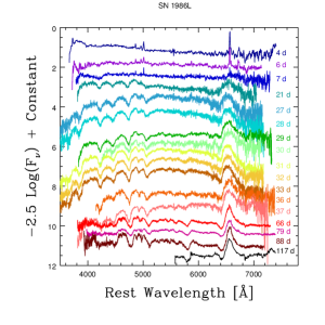
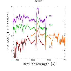
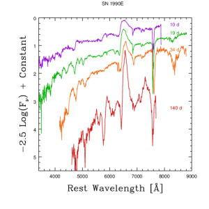
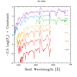
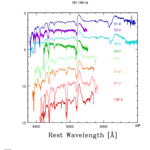
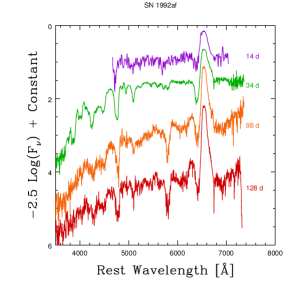
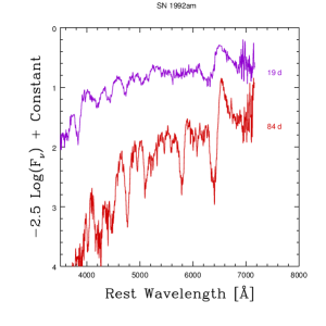
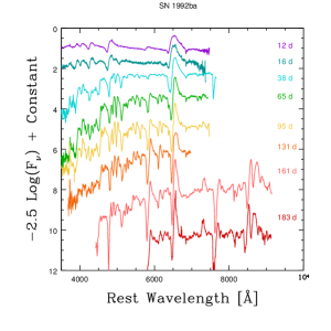
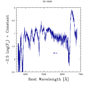
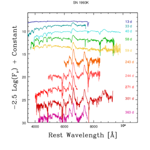
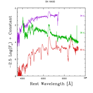
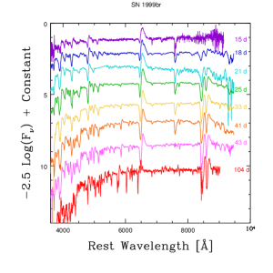
Figure 27.— Examples of SNe II spectra: SN 1986L, SN 1988A, SN 1990E, SN 1990K, SN 1991al, SN 1992af, SN 1992am, SN 1992ba, SN 1993A, SN 1993K, SN 1993S, SN 1999br.

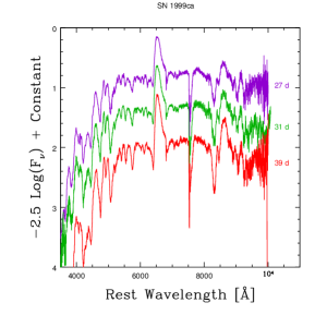
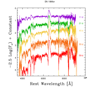
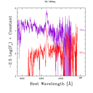
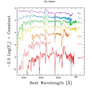
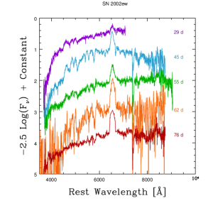
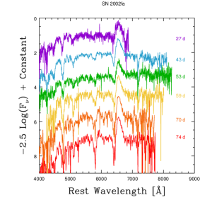
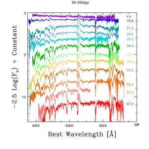
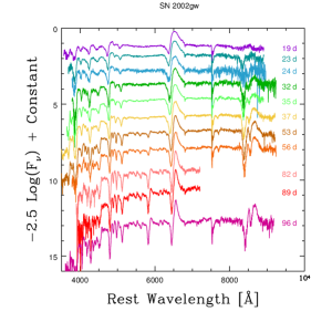
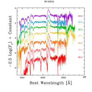
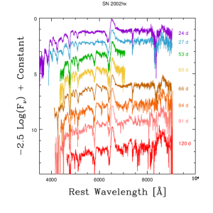
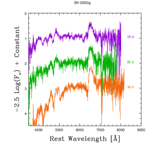
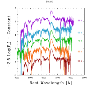
Figure 28.— Examples of SNe II spectra: SN 1999ca, SN 1999cr, SN 1999eg, SN 1999em, SN 2002ew, SN 2002fa, SN 200gd, SN 200gw, SN 2002hj, SN 2002hx, SN 2002ig, SN 210.

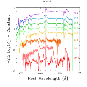
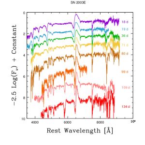
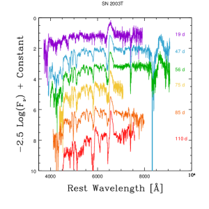
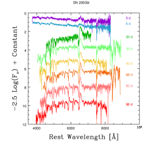
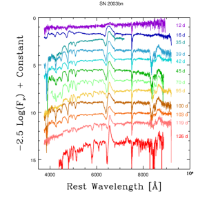
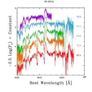
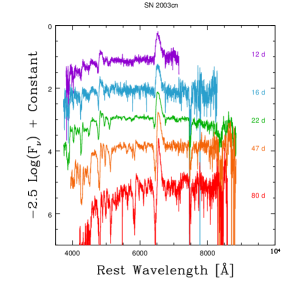
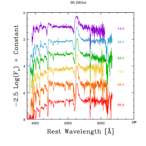
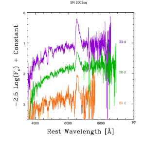
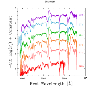
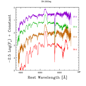
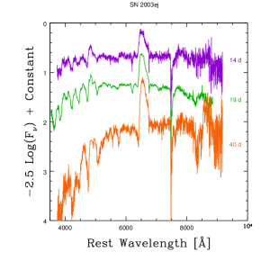
Figure 29.— Examples of SNe II spectra: SN 2003B, SN 2003E, SN 2003T, SN 2003bl, SN 2003bn, SN 2003ci, SN 2003cn, SN 2003cx, SN 2003dq, SN 2003ef, SN 2003eg, SN 2003ej.

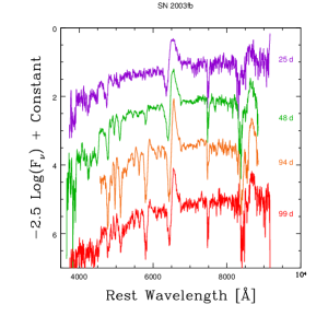
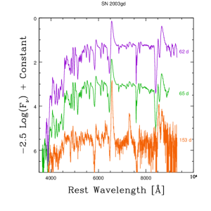
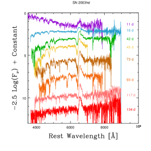
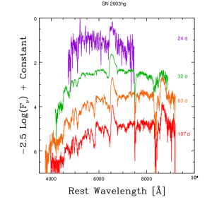
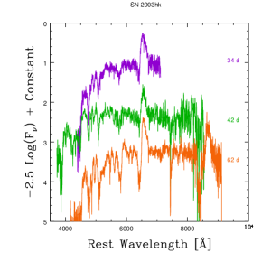
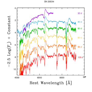
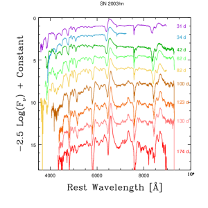
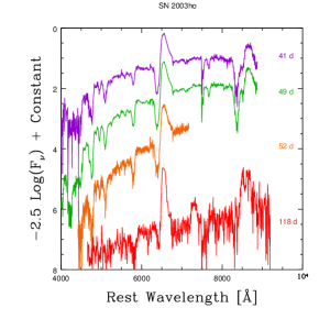
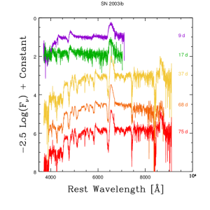
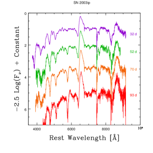
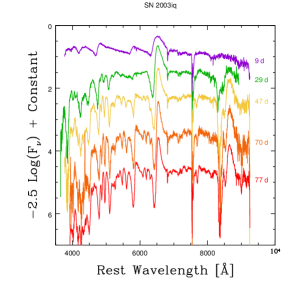
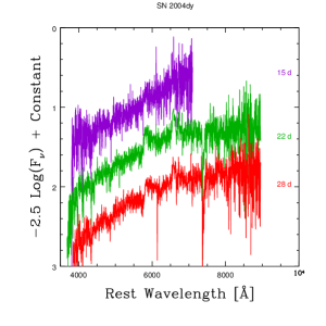
Figure 30.— Examples of SNe II spectra: SN 2003fb, SN 2003gd, SN 2003hd, SN 2003hg, SN 2003hk, SN 2003hl, SN 2003hn, SN 2003ho, SN 2003ib, SN 2003ip, SN 2003iq, SN 2004dy.

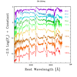
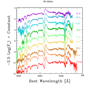
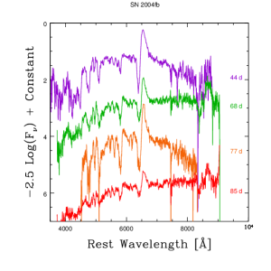
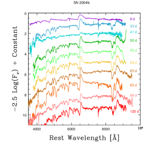
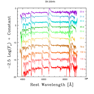
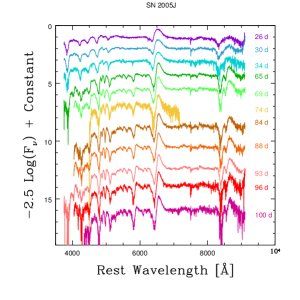
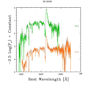
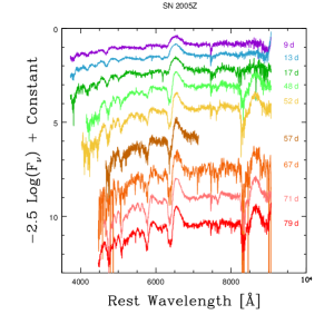
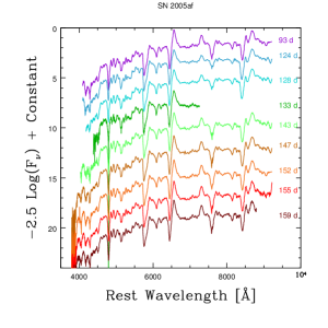
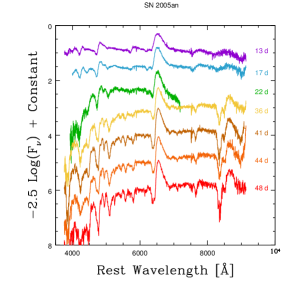
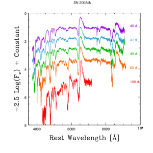
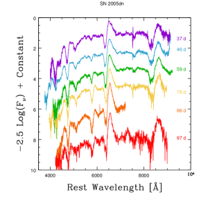
Figure 31.— Examples of SNe II spectra: SN 2004ej, SN 2004er, SN 2004fb, SN 2004fc, SN 2004fx, SN 2005J, SN 2005K, SN 2005Z, SN 2005af, SN 2005an, SN 2005dk, SN 2005dn.

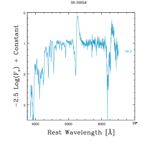
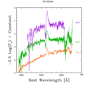
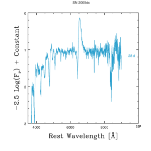
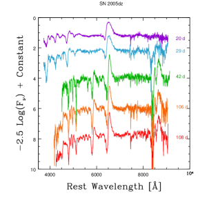
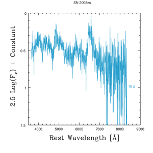
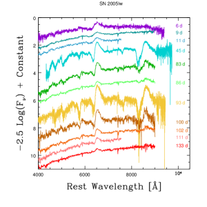
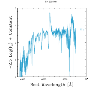
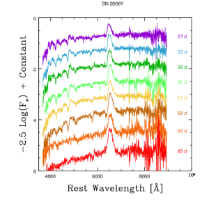
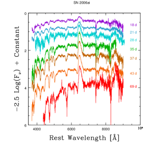
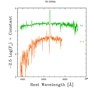
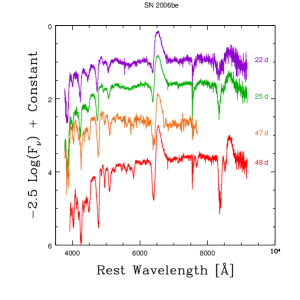
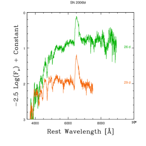
Figure 32.— Examples of SNe II spectra: SN 2005dt, SN 2005dw, SN 2005dx, SN 2005dz, SN 2005es, SN 2005lw, SN 2005me, SN 2006Y, SN 2006ai, SN 2006be, SN 2006be, SN 2006bl.

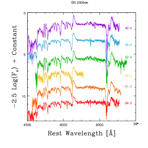
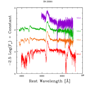
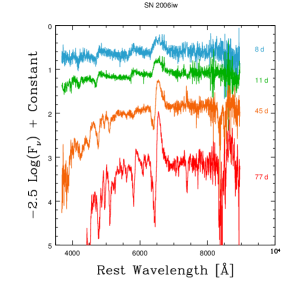
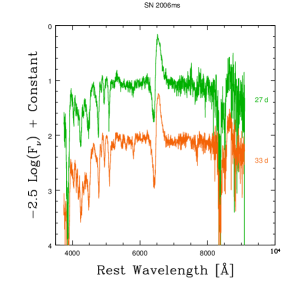
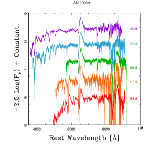
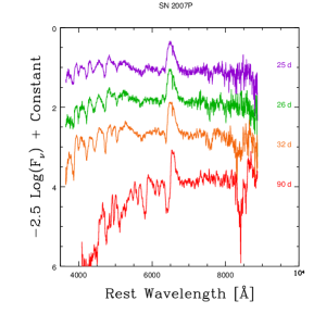
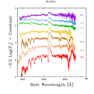
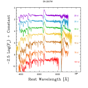
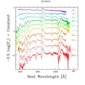
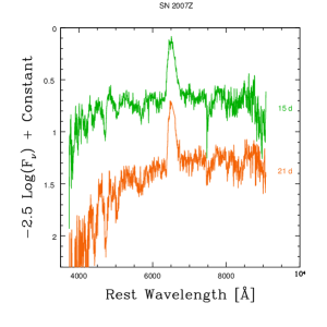
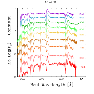
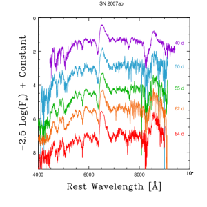
Figure 33.— Examples of SNe II spectra: SN 2006ee, SN 2006it, SN 2006iw, SN 2006ms, SN 2006qr, SN 2007P, SN 2007U, SN 2007W, SN 2007X, SN 2007Z, SN 2007aa, SN 2007ab.

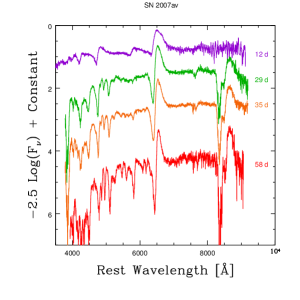
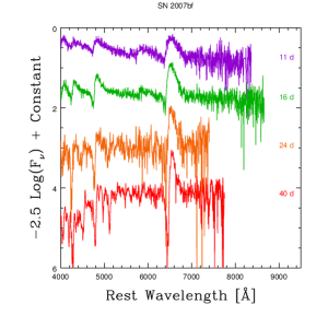
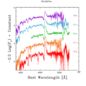
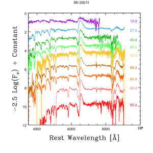
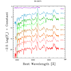
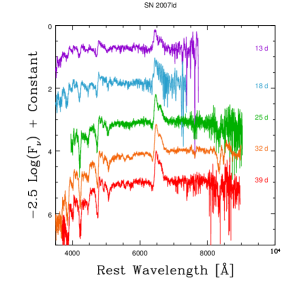
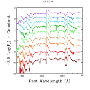
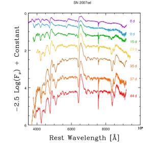
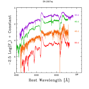
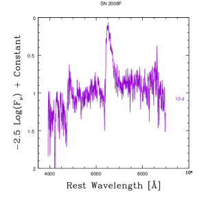
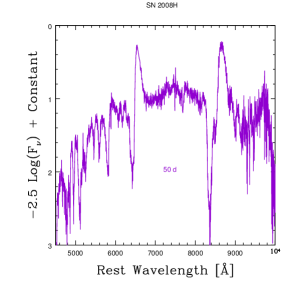
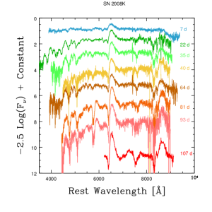
Figure 34.— Examples of SNe II spectra: SN 2007av, SN 2007bf, SN 2007hm, SN 2007il, SN 2007it, SN 2007ld, SN 2007oc, SN 2007od, SN 2007sq, SN 2008F, SN 2008H, SN 2008K.

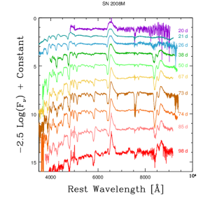
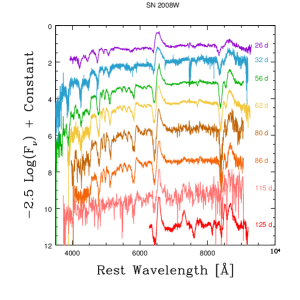
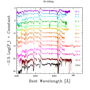
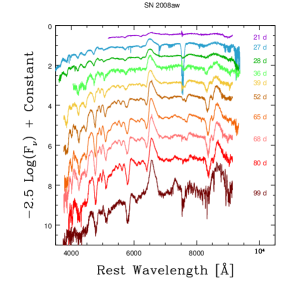
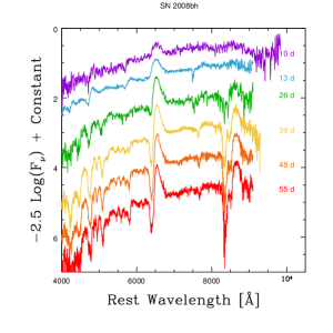
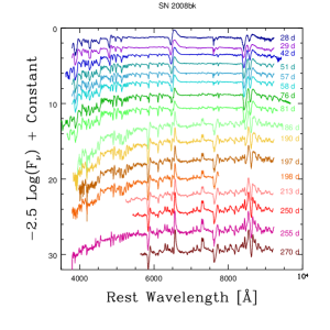
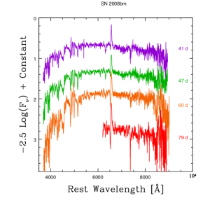
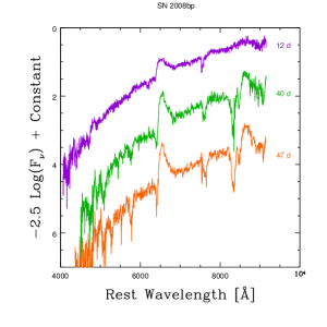
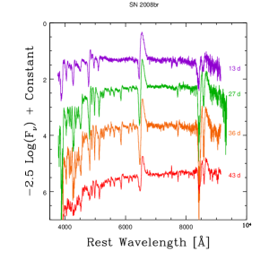
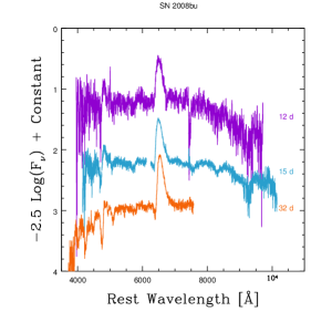
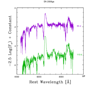
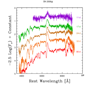
Figure 35.— Examples of SNe II spectra: SN 2008M, SN 2008W, SN 2008ag, SN 2008aw, SN 2008bh, SN 2008bk, SN 2008bm, SN 2008bp, SN 2008br, SN 2008bu, SN 2008ga, SN 2008gi.

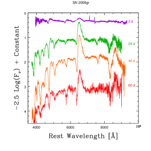
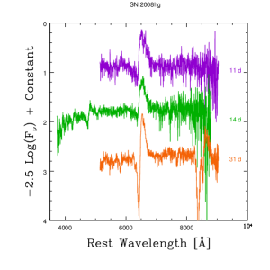
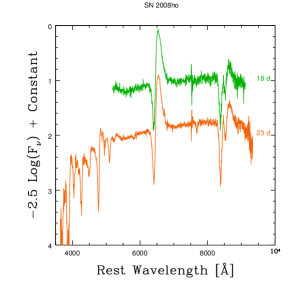
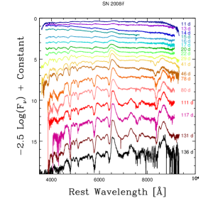
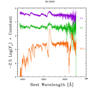
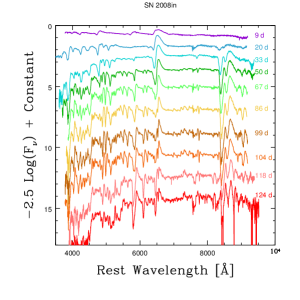
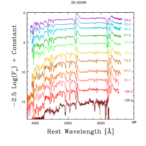
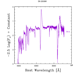
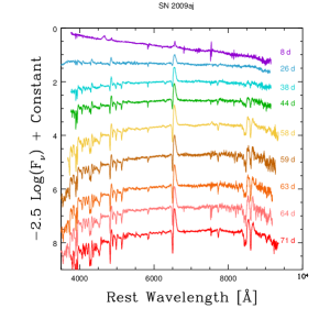
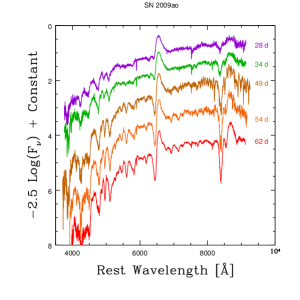
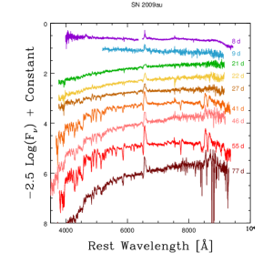
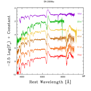
Figure 36.— Examples of SNe II spectra: SN 2008gr, SN 2008hg, SN 2008ho¸ SN 2008if, SN 2008il, SN 2008in, SN 2009N, SN 2009W, SN 2009aj, SN 2009ao, SN 2009au, SN 2009bu.

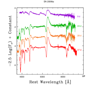
Figure 37.— Examples of SNe II spectra: SN 2009bz.

Appendix B SNID matches

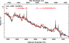
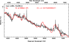
Figure 38.— Best spectral matching of SN 1986L using SNID. The plots show SN 1986L compared with SN 2006bp and SN 1999em at 6 and 7 days from explosion.

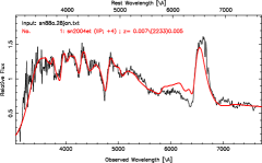
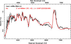
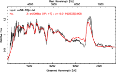
Figure 39.— Best spectral matching of SN 1988A using SNID. The plots show SN 1988A compared with SN 2004et, SN 1999em, SN 2006bp at 20, 15 and 16 days from explosion.

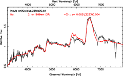
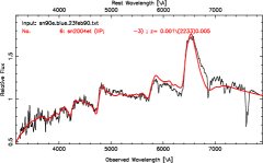
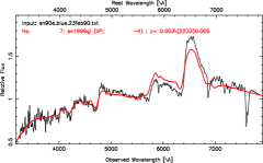
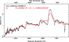
Figure 40.— Best spectral matching of SN 1990E using SNID. The plots show SN 1990E compared with SN 1999em, SN 2004et, SN 1999gi and SN2006bp at 7, 13, 8 and 9 days from explosion.

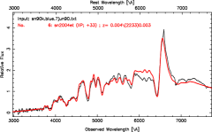
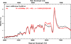
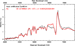
Figure 41.— Best spectral matching of SN 1990K using SNID. The plots show SN 1990K compared with SN 2004et, SN 2006bp , 1999em at 49, 58, and 37 days from explosion.

+

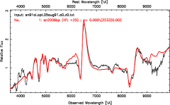
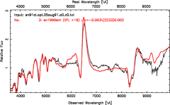
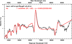
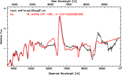
Figure 42.— Best spectral matching of SN 1991al using SNID. The plots show SN 1991al compared with SN 2006bp, SN 1999em, SN004et, and SN 2003iq at 34, 26, 36, and 29 days from explosion.

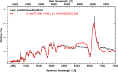
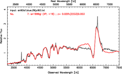
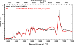
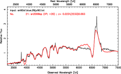
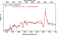
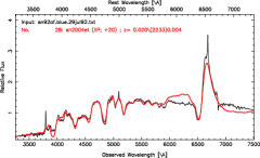
Figure 43.— Best spectral matching of SN 1992af using SNID. The plots show SN 1992af compared with SN 2007il, SN 199gi, SN 2003bn, SN 2006bp, SN 2003iq, and SN 2004et at 45, 31, 35, 29, 29, and 36 days from explosion.

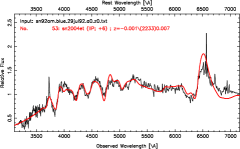
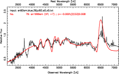
Figure 44.— Best spectral matching of SN 1992am using SNID. The plots show SN 1992am compared with SN 2004et and SN 1999em at 21 and 17 days from explosion.

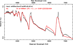
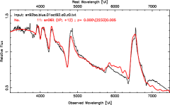
Figure 45.— Best spectral matching of SN 1992ba using SNID. The plots show SN 1992ba compared with SN 1999em and SN 2006it at 11 and 12 days from explosion.

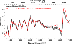
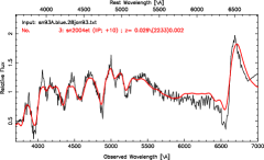
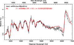
Figure 46.— Best spectral matching of SN 1993A using SNID. The plots show SN 1993A compared with SN 1999em, SN 2004et, SN 2006bb at 21, 36, and 23 days from explosion.

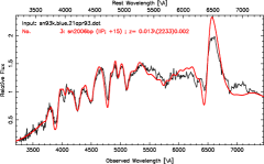
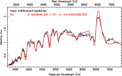
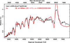
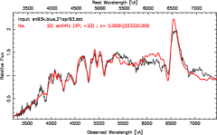
Figure 47.— Best spectral matching of SN 1993K using SNID. The plots show SN 1993K compared with SN 2006bp, SN 2004et, SN 1999em, and SN 2004fc at 24, 28, 21, and 33 days from explosion.

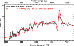
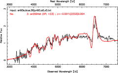
Figure 48.— Best spectral matching of SN 1993S using SNID. The plots show SN 1993S compared with SN 2006bp and SN 2004et at 29 and 39 days from explosion.

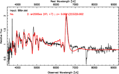
Figure 49.— Best spectral matching of SN 1999br using SNID. The plots show SN 1999br compared with SN 1999br at 13 days from explosion.

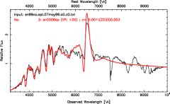
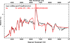
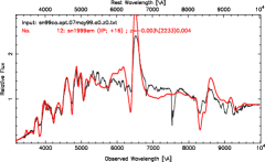
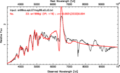
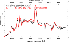
Figure 50.— Best spectral matching of SN 1999ca using SNID. The plots show SN 1999ca compared with SN 2006bp, SN 2003iq, SN 1999em, SN 1999gi, and 2007oc at 29, 29, 26, 31 and 21 days from explosion.

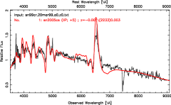
Figure 51.— Best spectral matching of SN 1999cr using SNID. The plots show SN 1999cr compared with SN 2005cs at 11 days from explosion.

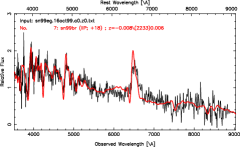
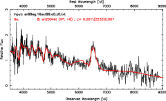
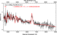
Figure 52.— Best spectral matching of SN 1999eg using SNID. The plots show SN 1999eg compared with SN 1999br, SN 2004et, and SN 2005cs at 18, 22, and 13 days from explosion.

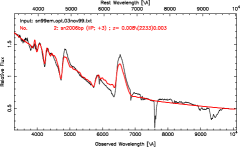
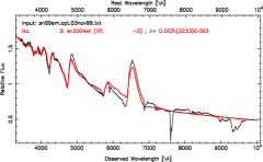
Figure 53.— Best spectral matching of SN 1999em using SNID. The plots show SN 1999em compared with SN 2006bp and SN 2004et at 12 and 13 days from explosion.

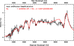
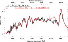
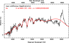
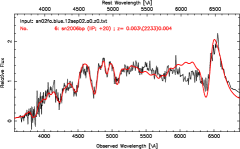
Figure 54.— Best spectral matching of SN 2002fa using SNID. The plots show SN 2002fa compared with SN 2004et, SN 1999em, SN 1992H, SN 2006bp, and SN 1999gi at 31, 21, 30, 29, and 31 days from explosion.

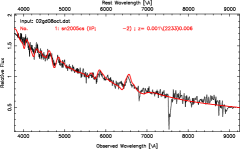
Figure 55.— Best spectral matching of SN 2002gd using SNID. The plots show SN 2002gd compared with SN 2005cs at 4 days from explosion.

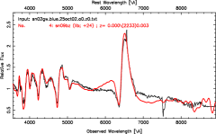
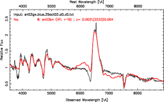
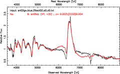
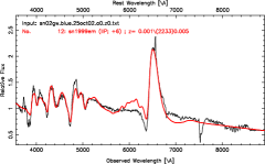
Figure 56.— Best spectral matching of SN 2002gw using SNID. The plots show SN 2002gw compared with SN 2009bz, SN 2003bn, SN 2005dz, and SN 1999em at 24, 16, 20, and 16 days from explosion.

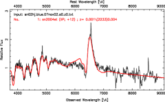
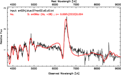
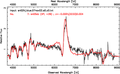
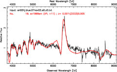
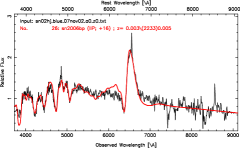
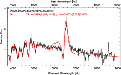
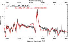
Figure 57.— Best spectral matching of SN 2002hj using SNID. The plots show SN 2002hj compared with SN 2004et, SN 2009bz, SN 2005dz, SN 1999em, SN 2006bp, SN 1999gi, and SN 2003iq at 28, 28, 29, 21, 25, 31, and 29 days from explosion.

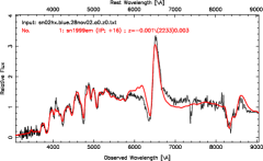
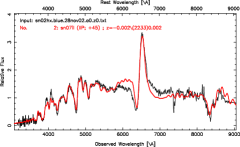
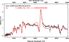
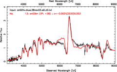
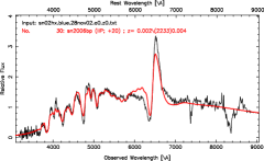
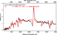
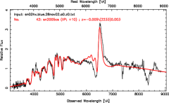
Figure 58.— Best spectral matching of SN 2002hx using SNID. The plots show SN 2002hx compared with SN 1999em, SN 2007il, SN 2009bz, SN 2003bn, SN 2006bp, SN 1999br, and SN 2005cs at 26, 45, 37, 39, 29, 25, and 16 days from explosion.

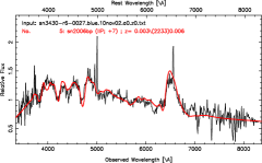
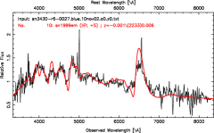
Figure 59.— Best spectral matching of SN 2002ig using SNID. The plots show SN 2002ig compared with SN 2004et, SN 2006bp, and SN 1999em at 22, 16, and 15 days from explosion.

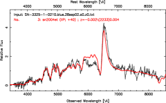
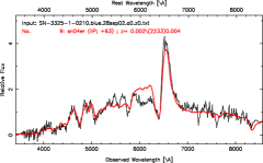
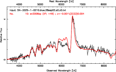
Figure 60.— Best spectral matching of SN 210 using SNID. The plots show SN 210 compared with SN 2004et, SN 2004er, and SN 2006bp at 56, 63, and 58 days from explosion.

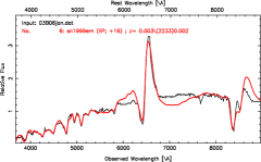
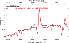
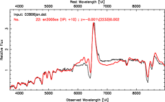
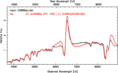
Figure 61.— Best spectral matching of SN 2003B using SNID. The plots show SN 2003B compared with SN 2007il, SN 1999em, SN 2003bn, SN 2005cs, and SN 2006bp at 45, 26, 39, 16, and 34 days from explosion.

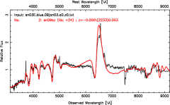
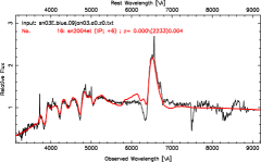
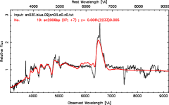
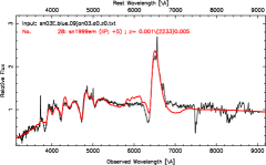
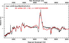
Figure 62.— Best spectral matching of SN 2003E using SNID. The plots show SN 2003E compared with SN 2009bz, SN 2004et, SN 2006bp, SN 1999em, and SN 2003bn at 24, 22, 16, 15, and 16 days from explosion.

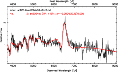
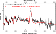
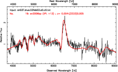
Figure 63.— Best spectral matching of SN 2003T using SNID. The plots show SN 2003T compared with SN 2004et, SN 1999em, and SN 2006bp at 26, 19, and 22 days from explosion.

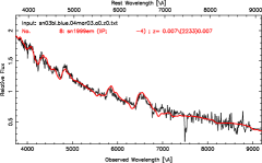
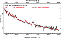
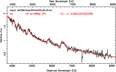
Figure 64.— Best spectral matching of SN 2003bl using SNID. The plots show SN 2003bl compared with SN 1999em, SN 2005cs, and SN 1999gi at 6, 4, and 8 days from explosion.

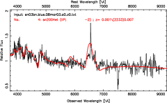
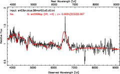
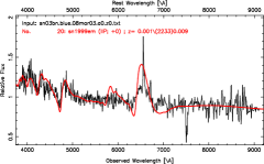
Figure 65.— Best spectral matching of SN 2003bn using SNID. The plots show SN 2003bn compared with SN 2004et, SN 2006bp, and SN 1999em at 14, 13, and 10 days from explosion.

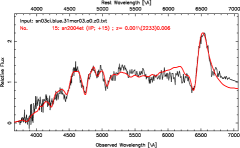
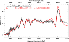
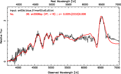
Figure 66.— Best spectral matching of SN 2003ci using SNID. The plots show SN 2003ci compared with SN 2004et, SN 1999em, and SN 2006bp at 31, 21, and 25 days from explosion.

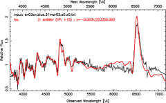
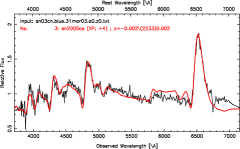
Figure 67.— Best spectral matching of SN 2003cn using SNID. The plots show SN 2003cn compared with SN 1999br and SN 2005cs at 15 and 10 days from explosion.

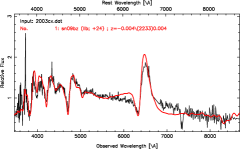
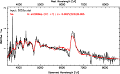
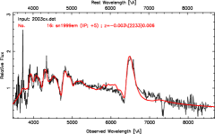
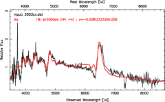
Figure 68.— Best spectral matching of SN 2003cx using SNID. The plots show SN 2003cx compared with SN 2009bz, SN 2006bp, SN 1999em, and SN 2005cs at 24, 16, 15, and 10 days from explosion.

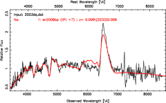
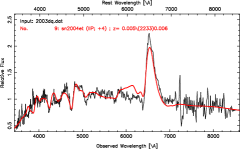
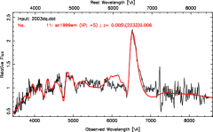
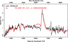
Figure 69.— Best spectral matching of SN 2003dq using SNID. The plots show SN 2003dq compared with SN 2006bp, SN 2004et, SN 1999em, and SN 2006Y at 16, 20, 15, 51 days from explosion.

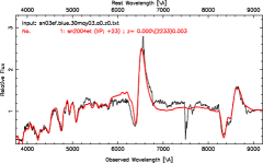
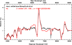
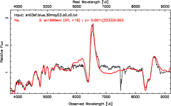
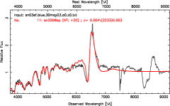
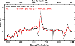
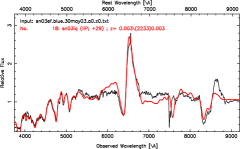
Figure 70.— Best spectral matching of SN 2003ef using SNID. The plots show SN 2003ef compared with SN 2004et, SN 2003bn, SN 1999em, SN 2006bp, SN 2004fc, and SN 2003iq at 39, 39, 26, 29, 33 days from explosion.

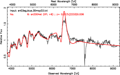
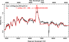
Figure 71.— Best spectral matching of SN 2003eg using SNID. The plots show SN 2003eg compared with SN 2004et, and SN 2009ao at 22 and 28 days from explosion.

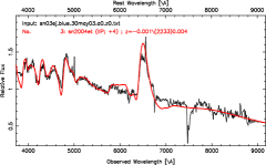
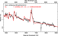
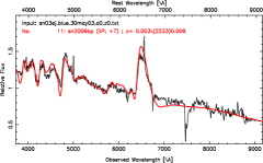
Figure 72.— Best spectral matching of SN 2003ej using SNID. The plots show SN 2003ej compared with SN 2004et, SN 2005cs, and SN 2006bp at 20, 8, and 16 days from explosion.

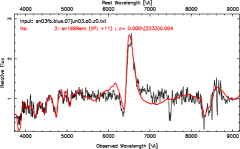
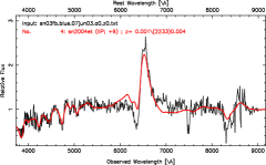
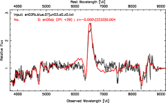
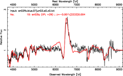
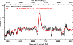
Figure 73.— Best spectral matching of SN 2003fb using SNID. The plots show SN 2003fb compared with SN 1999em, SN 2004et, SN 2005dz, SN 2003iq, and SN 2006bp at 21, 25, 29, 29, and 22 days from explosion.

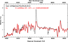
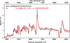
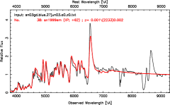
Figure 74.— Best spectral matching of SN 2003gd using SNID. The plots show SN 2003gd compared with SN 2005cs, SN 2006ee, and SN 1999em at 63, 52, and 72 days from explosion.

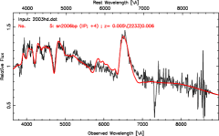
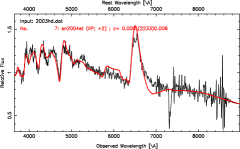
Figure 75.— Best spectral matching of SN 2003hd using SNID. The plots show SN 2003hd compared with SN 2006b and SN 2004et at 13 and 18 days from explosion.

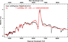
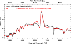
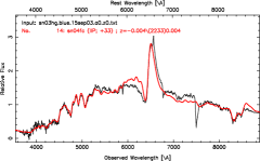
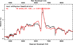
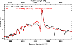
Figure 76.— Best spectral matching of SN 2003hg using SNID. The plots show SN 2003hg compared with SN 2006bp, SN 2004et, SN 2004fc, SN 2003iq, and SN 1999gi at 29, 31, 33, 29, and 31 days from explosion.

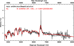
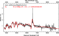
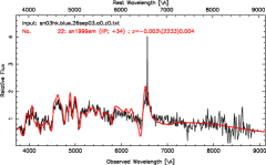
Figure 77.— Best spectral matching of SN 2003hk using SNID. The plots show SN 2003hk compared with SN 2004et, SN 1999gi, and SN 1999em at 41, 41, and 44 days from explosion.

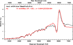
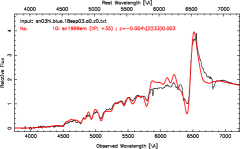
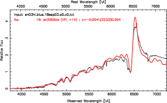
Figure 78.— Best spectral matching of SN 2003hl using SNID. The plots show SN 2003hl compared with SN 2006bp, SN 1999em, and SN 2005cs at 34, 45, and 20 days from explosion.

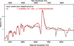
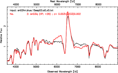
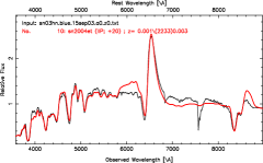
Figure 79.— Best spectral matching of SN 2003hn using SNID. The plots show SN 2003hn compared with SN 2006bp, SN 2003iq, and SN 2004et at 29, 29, and 36 days from explosion.

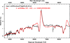
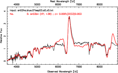
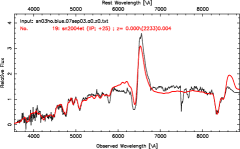
Figure 80.— Best spectral matching of SN 2003ho using SNID. The plots show SN 2003ho compared with SN 2006bp, SN 2003bn, and SN 2004et at 43, 39, and 41 days from explosion.

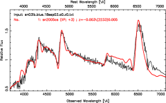
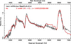
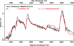
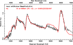
Figure 81.— Best spectral matching of SN 2003ib using SNID. The plots show SN 2003ib compared with SN 2005cs, SN 2006it, SN 2004et, and SN 1999em at 9, 12, 15, and 12 days from explosion.

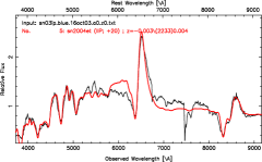
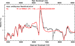
Figure 82.— Best spectral matching of SN 2003ip using SNID. The plots show SN 2003ip compared with SN 2004et and SN 1999em at 36 and 26 days from explosion.

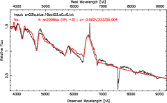
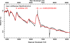
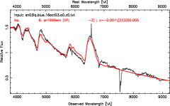
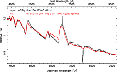
Figure 83.— Best spectral matching of SN 2003iq using SNID. The plots show SN 2003iq compared with SN 2006bp, SN 2004et, SN 1999em, and SN 2004fc at 13, 12, 7, and 9 days from explosion.

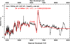
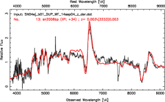
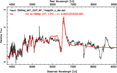
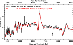
Figure 84.— Best spectral matching of SN 2004ej using SNID. The plots show SN 2004ej compared with SN1999em , SN 2006bp, SN 1999gi, and SN 2004et at 37, 43, 36, and 39 days from explosion.

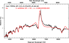
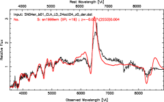
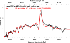
Figure 85.— Best spectral matching of SN 2004er using SNID. The plots show SN 2004er compared with SN 2004et, SN 1999em, and SN 2006bp at 31, 36, and 25 days from explosion.

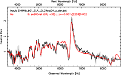
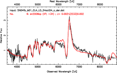
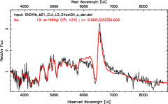
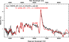
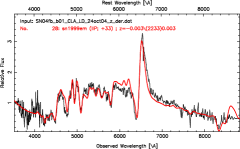
Figure 86.— Best spectral matching of SN 2004fb using SNID. The plots show SN 2004fb compared with SN 2004et, SN 2006bp, SN 1999gi, SN 2003iq, and SN 1999em at 51, 43, 36, 47, and 43 days from explosion.

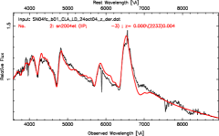
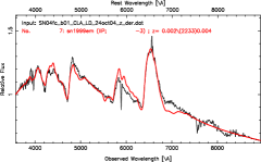
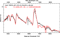
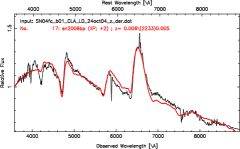
Figure 87.— Best spectral matching of SN 2004fc using SNID. The plots show SN 2004fc compared with SN 2004et, SN 1999em, SN 2003iq, and SN 2006bp at 13, 7, 9, and 11 days from explosion.

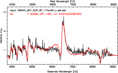
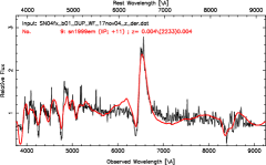
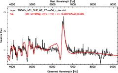
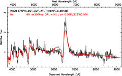
Figure 88.— Best spectral matching of SN 2004fx using SNID. The plots show SN 2004fx compared with SN 2005dz, SN 1999em, SN 1999gi, and SN 2006bp at 29, 21, 31, and 23 days from explosion.

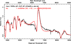
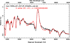
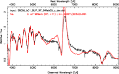
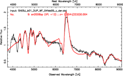
Figure 89.— Best spectral matching of SN 2005J using SNID. The plots show SN 2005J compared with SN 2004et, SN 2004er, SN 1999em, and SN 2006bp at 31, 31, 21, and 22 days from explosion.

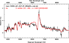
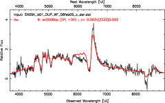
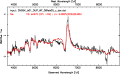
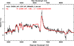
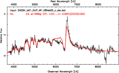
Figure 90.— Best spectral matching of SN 2005K using SNID. The plots show SN 2005K compared with SN 2003bn, SN 2006bp, SN 2007il, SN 2006it, and SN 1999gi at 39, 43, 45, 36, and 36 days from explosion.

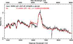
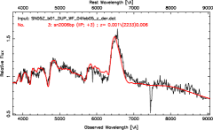
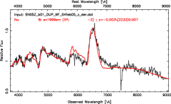
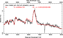
Figure 91.— Best spectral matching of SN 2005Z using SNID. The plots show SN 2005Z compared with SN 2004fc, SN 2006bp, SN 1999em, and 2004et at 9, 11, 8 and 13 days from explosion.

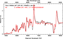
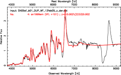
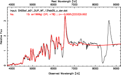
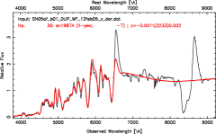
Figure 92.— Best spectral matching of SN 2005af using SNID. The plots show SN 2005af compared with SN 2006ee, SN 1999em, SN 1999gi, and 1987A at 94, 111, 90, and 78 days from explosion.

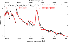
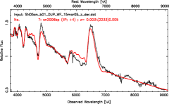
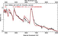
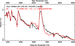
Figure 93.— Best spectral matching of SN 2005an using SNID. The plots show SN 2005an compared with SN 2004et, SN 2006bp, SN 1999em, and SN 2006it at 15, 13, 10, and 12 days from explosion.

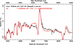
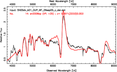
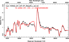
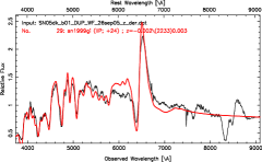
Figure 94.— Best spectral matching of SN 2005dk using SNID. The plots show SN 2005dk compared with SN 2004et, SN 2006bp, SN 2003bn, and SN 1999gi at 39,34, and 36 days from explosion.

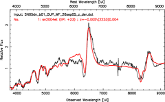
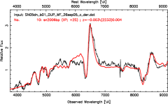
Figure 95.— Best spectral matching of SN 2005dn using SNID. The plots show SN 2005dn compared with SN 2004et and SN 2006bp at 39 and 34 days from explosion.

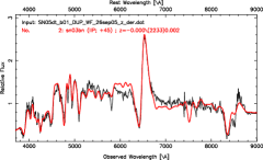
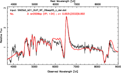
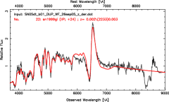
Figure 96.— Best spectral matching of SN 2005dt using SNID. The plots show SN 2005dt compared with SN 2003bn, SN 2006bp, and SN 1999gi at 45, 43, and 36 days from explosion.

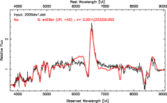
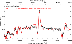
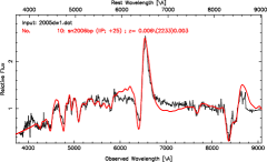
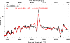
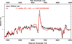
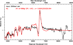
Figure 97.— Best spectral matching of SN 2005dw using SNID. The plots show SN 2005dw compared with SN 1999em, SN 2003bn, SN 2004et, SN 2006bp, SN 2004fc, SN 2006iw, and SN 1999gi at 36, 42, 39, 34, 33, 45, and 36 days from explosion.

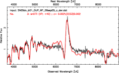
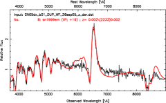
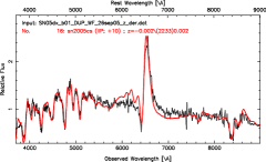
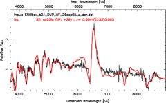
Figure 98.— Best spectral matching of SN 2005dx using SNID. The plots show SN 2005dx compared with SN 2007il, SN 1999em, SN 2005cs, and SN 2003iq at 40, 26, 16, and 29 days from explosion.

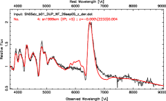
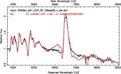
Figure 99.— Best spectral matching of SN 2005dz using SNID. The plots show SN 2005dz compared with SN 1999em and SN 2003bn at 15 and 16 days from explosion.

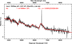
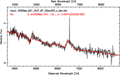
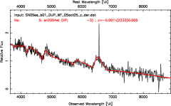
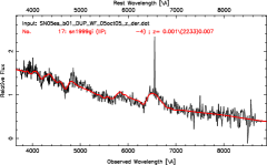
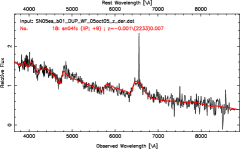
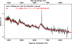
Figure 100.— Best spectral matching of SN 2005es using SNID. The plots show SN 2005es compared with SN 1999em, SN 2006bp, SN 2004et, SN 1999gi, SN 2004fc, and SN 2006iw at 8, 12, 13, 8, 9, and 11 days from explosion.

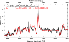
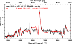
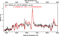
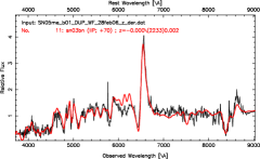
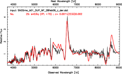
Figure 101.— Best spectral matching of SN 2005me using SNID. The plots show SN 2005me compared with SN 2004et, SN 2008il, SN 2006bp, SN 2003bn, and SN 2003iq at 74, 63, 74, 70 and 70 days from explosion.

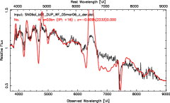
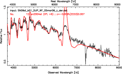
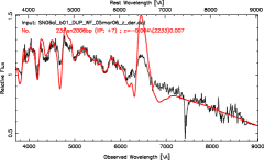
Figure 102.— Best spectral matching of SN 2006ai using SNID. The plots show SN 2006ai compared with SN 2003bn, SN 2004et, and SN 2006bp at 16, 22, and 16 days from explosion.

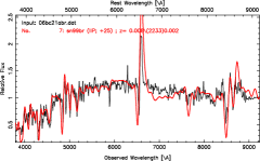
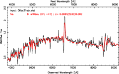
Figure 103.— Best spectral matching of SN 2006bc using SNID. The plots show SN 2006bc compared with SN 1999br and SN 2009au at 25 and 41 days from explosion.

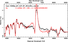
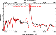
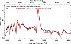
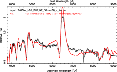
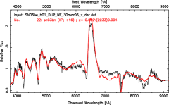
Figure 104.— Best spectral matching of SN 2006be using SNID. The plots show SN 2006be compared with SN 2005dz, SN 1999em, SN 2006bp, SN 2009bz, and SN 2003bn at 29, 21, 22 24, and 16 days from explosion.

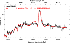
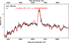
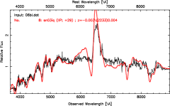
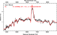
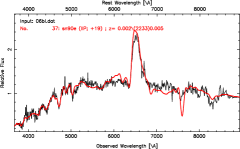
Figure 105.— Best spectral matching of SN 2006bl using SNID. The plots show SN 2006bl compared with SN 2004et, SN 2004er, SN 1999em, SN 2003iq, SN 2006bp, SN 1999gi, and SN 1990E at 26, 31, 21, 29, 22, 31 and 19 days from explosion.

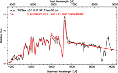
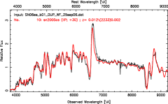
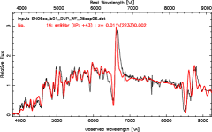
Figure 106.— Best spectral matching of SN 2006ee using SNID. The plots show SN 2006ee compared with SN 1999em, SN 2005cs, and SN 1999br at 45, 36, and 43 days from explosion.

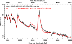
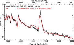
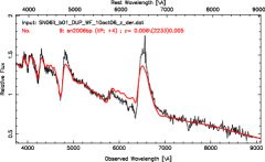
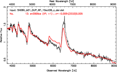
Figure 107.— Best spectral matching of SN 2006it using SNID. The plots show SN 2006it compared with SN 1999em, SN 2004et, SN 2006bp, and SN 2005cs at 12, 17, 13 and 7 days from explosion.

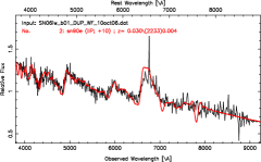
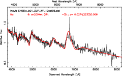
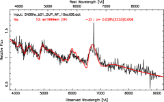
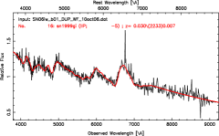
Figure 108.— Best spectral matching of SN 2006iw using SNID. The plots show SN 2006iw compared with SN 1990E, SN 2004et, SN 1999em, and SN 1999gi at 10, 13, 7, and 7 days from explosion.

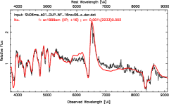
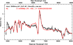
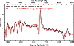
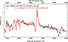
Figure 109.— Best spectral matching of SN 2006ms using SNID. The plots show SN 2006ms compared with SN 1999em, SN 2006bp, SN 2005cs, and SN 1999gi at 26, 34, 19, smf 31 days from explosion.

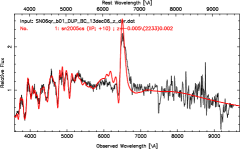
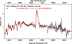
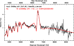
Figure 110.— Best spectral matching of SN 2006qr using SNID. The plots show SN 2006qr compared with SN 2005cs, SN 2004et, and SN 2006bp at 16, 26, and 24 days from explosion.

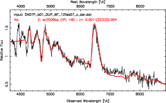
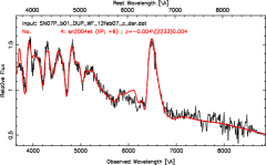
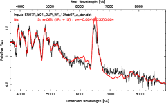
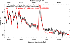
Figure 111.— Best spectral matching of SN 2007P using SNID. The plots show SN 2007P compared with SN 2006bp, SN 2004et, SN 2006it, and SN 2005dz at 17. 22, 15, and 20 days from explosion.

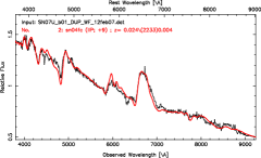
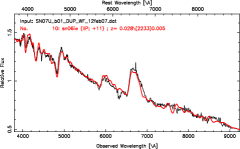
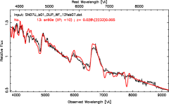
Figure 112.— Best spectral matching of SN 2007U using SNID. The plots show SN 2007U compared with SN 2004fc, SN 2006iw, and SN 1990E at 9, 11, and 10 days from explosion.

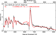
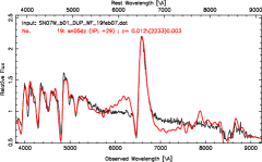
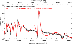
Figure 113.— Best spectral matching of SN 2007W using SNID. The plots show SN 2007W compared with SN 2005cs, SN 2005dz, and SN 1999em at 11, 29, and 21 days from explosion.

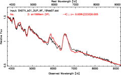
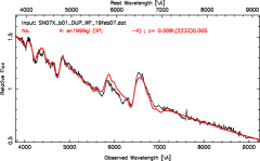
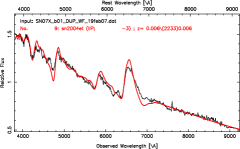
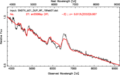
Figure 114.— Best spectral matching of SN 2007X using SNID. The plots show SN 2007X compared with SN 1999em, SN 1999gi, SN 2004et, and SN 2006bp at 6, 8, 13, and 7 days from explosion.

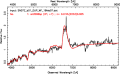
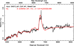
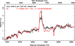
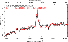
Figure 115.— Best spectral matching of SN 2007Z using SNID. The plots show SN 2007Z compared with SN 2006bp, SN 2004et, SN 2003bn, and SN 2006it at 16, 17, 16, and 12 days from explosion.

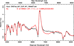
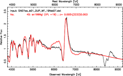
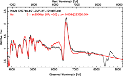
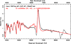
Figure 116.— Best spectral matching of SN 2007aa using SNID. The plots show SN 2007aa compared with SN 1999em, SN 1999gi, SN 2006bp, and SN 2005cs at 21, 31, 29, and 15 days from explosion.

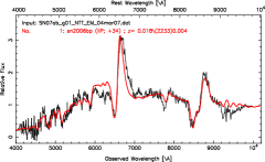
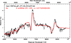
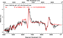
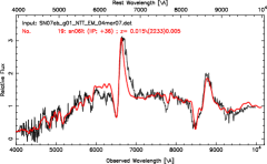
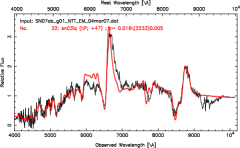
Figure 117.— Best spectral matching of SN 2007ab using SNID. The plots show SN 2007ab compared with SN 2006bp, SN 2004et, SN 1999em, SN 2006it and SN 2003iq at 43, 39, 43, 36, and 47 days from explosion.

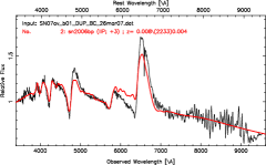
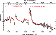
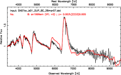
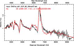
Figure 118.— Best spectral matching of SN 2007av using SNID. The plots show SN 2007av compared with SN 2006bp, SN 2004et, SN 1999em, and SN 2006it at 12, 13, 10, and 12 days from explosion.

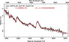
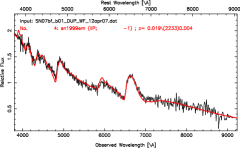
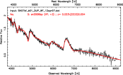
Figure 119.— Best spectral matching of SN 2007bf using SNID. The plots show SN 2007bf compared with SN 2004et, SN 1999em, and SN 2006bp at 13, 9, and 12 days from explosion.

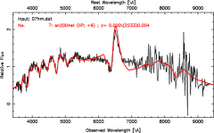
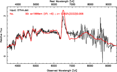
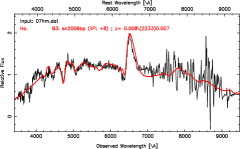
Figure 120.— Best spectral matching of SN 2007hm using SNID. The plots show SN 2007hm compared with SN 2004et, SN 1999em, and SN 2006bp at 25, 16, and 17 days from explosion.

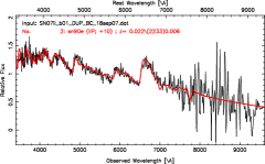
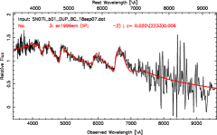
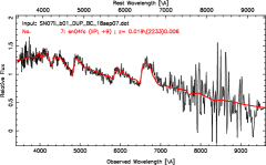
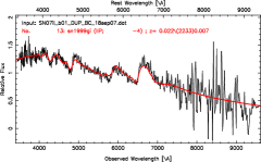
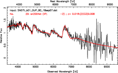
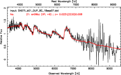
Figure 121.— Best spectral matching of SN 2007il using SNID. The plots show SN 2007il compared with SN 1990E, SN 1999em, SN 2004fc, SN 1999gi, SN 2004et, and SN 2009bz at 10, 8, 9, 8, 14, and 9 days from explosion.

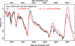
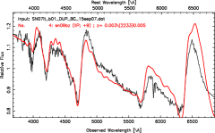
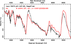
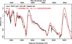
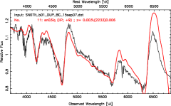
Figure 122.— Best spectral matching of SN 2007it using SNID. The plots show SN 2007it compared with SN 2004et, SN 2009bz, SN 2004fc, SN 2006bp, and SN 2003iq at 13, 9, 9, 12, and 9 days from explosion.

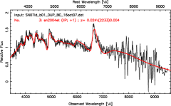
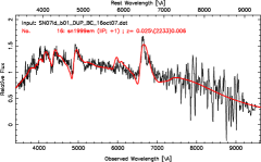
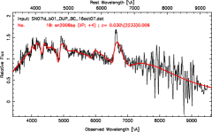
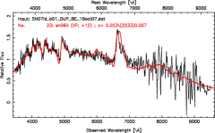
Figure 123.— Best spectral matching of SN 2007ld using SNID. The plots show SN 2007ld compared with SN 2004et, SN 1999em, SN 2006bp, and SN 2006it at 17, 11, 13m and 12 days from explosion.

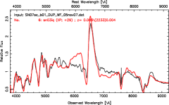
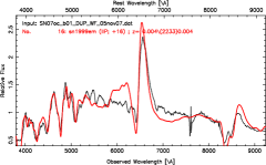
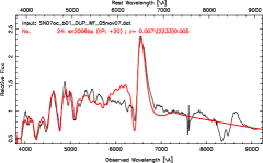
Figure 124.— Best spectral matching of SN 2007oc using SNID. The plots show SN 2007oc compared with SN 2003iq, SN 1999em, and SN 2006bp at 29, 26, and 29 days from explosion.

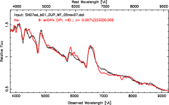
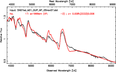
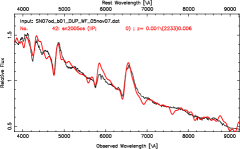
Figure 125.— Best spectral matching of SN 2007od using SNID. The plots show SN 2007od compared with SN 2004et, SN 2004fc, SN 1999em, and SN 2005cs at 13, 9, 8, and 6 days from explosion.

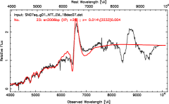
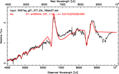
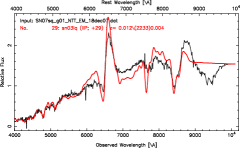
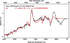
Figure 126.— Best spectral matching of SN 2007sq using SNID. The plots show SN 2007sq compared with SN 2006bp, SN 2004et, SN 2003iq, and SN 2004er at 29, 31, 29, and 31 days from explosion.

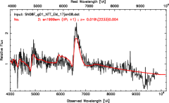
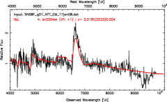
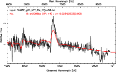
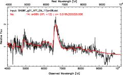
Figure 127.— Best spectral matching of SN 2008F using SNID. The plots show SN 2008F compared with SN 1999em, SN 2004et, SN 2006bp, and SN 2006it at 11, 17, 13, and 12 days from explosion.

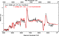
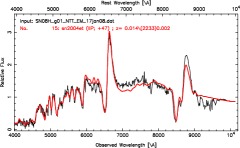
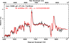
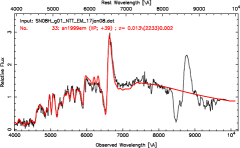
Figure 128.— Best spectral matching of SN 2008H using SNID. The plots show SN 2008H compared with SN 2004fc, SN 2006ee, SN 2004et, SN 2005cs, and SN 1999em at 59, 42, 63, 36, and 49 days from explosion.

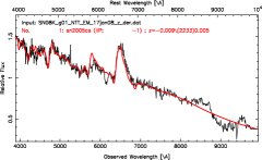
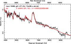
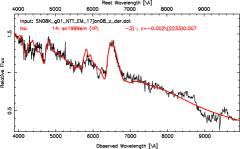
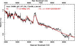
Figure 129.— Best spectral matching of SN 2008K using SNID. The plots show SN 2008K compared with SN 2005cs, SN 2004fc, SN 1999em, and SN 1999gi at 5, 9, 7 and 8 days from explosion.

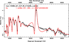
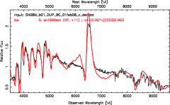
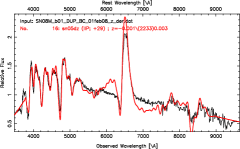
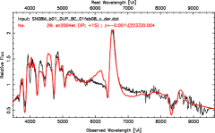
Figure 130.— Best spectral matching of SN 2008M using SNID. The plots show SN 2008M compared with SN 2009bz, SN 1999em, SN 2005dz, and SN 2004et at 28, 21, 24, and 26 days from explosion.

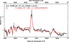
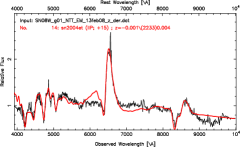
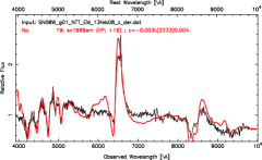
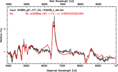
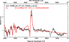
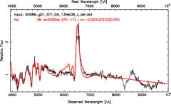
Figure 131.— Best spectral matching of SN 2008W using SNID. The plots show SN 2008W compared with SN 2009ao, SN 2004et, SN 1999em, SN 2006bp, SN 1999gi, and SN 2005cs at 28, 31, 26, 26, 31, and 17 days from explosion.

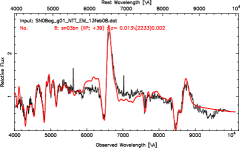
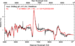
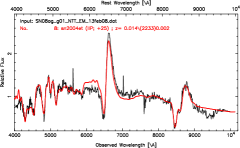
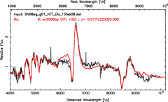
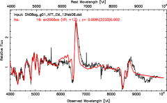
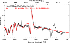
Figure 132.— Best spectral matching of SN 2008ag using SNID. The plots show SN 2008ag compared with SN 2003bn, SN 1999em, SN 2004et, SN 2006bp, SN 2005cs, and SN 1999gi at 39, 26, 41, 34, 19, and 31 days from explosion.

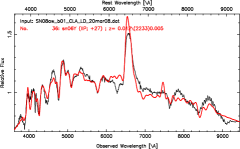
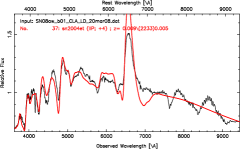
Figure 133.— Best spectral matching of SN 2008aw using SNID. The plots show SN 2008aw compared with SN 2006Y and SN 2004et at 27 and 20 days from explosion.

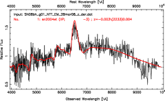
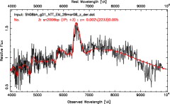
Figure 134.— Best spectral matching of SN 2008bh using SNID. The plots show SN 2008bh compared with SN 2004et and SN 2006bp at 13 and 12 days from explosion.

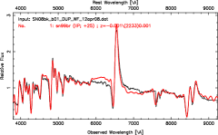
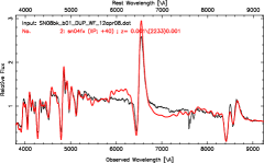
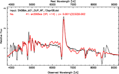
Figure 135.— Best spectral matching of SN 2008bk using SNID. The plots show SN 2008bk compared with SN 1999br, SN 2004fx, and SN 2005cs at 25, 40, and 20 days from explosion.

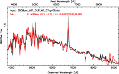
Figure 136.— Best spectral matching of SN 2008bm using SNID. The plots show SN 2008bm compared with SN 2009au at 41 days from explosion.

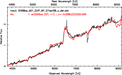
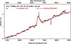
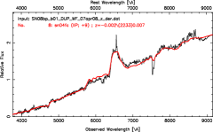
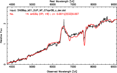
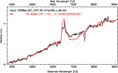
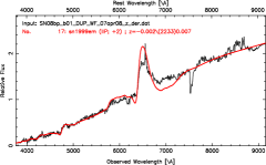
Figure 137.— Best spectral matching of SN 2008bp using SNID. The plots show SN 2008bp compared with SN 2005cs, SN 2004et, SN 2004fc, SN 2003iq, SN 2006it, and SN 1999em at 7, 13, 9, 9, 12, and 12 days from explosion.

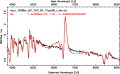
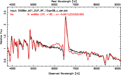
Figure 138.— Best spectral matching of SN 2008br using SNID. The plots show SN 2008br compared with SN 2005cs and SN 1999br at 16, 18 days from explosion.

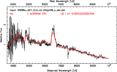
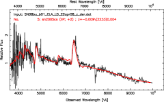
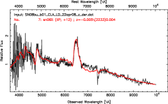
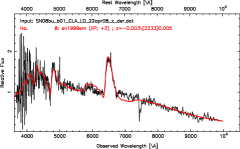
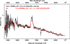
Figure 139.— Best spectral matching of SN 2008bu using SNID. The plots show SN 2008bu compared with SN 2004et, SN 2005cs, SN 2006it, SN 1999em, and SN 2006bp at 14, 8, 12, 12, and 13 days from explosion.

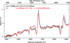
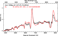
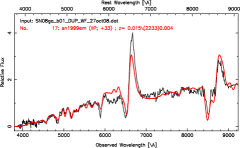
Figure 140.— Best spectral matching of SN 2008ga using SNID. The plots show SN 2008ga compared with SN 2006bp, SN 2007oc, and SN 1999em at 58, 64, and 43 days from explosion.

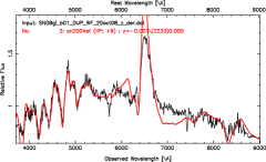
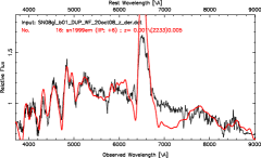
Figure 141.— Best spectral matching of SN 2008gi using SNID. The plots show SN 2008gi compared with SN 2004et and SN 1999em at 25 and 16 days from explosion.

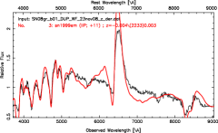
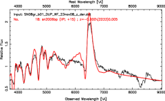
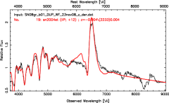
Figure 142.— Best spectral matching of SN 2008gr using SNID. The plots show SN 2008gr compared with SN 1999em, SN 2006bp, and SN 2004et at 21, 24, and 28 days from explosion.

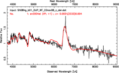
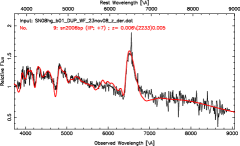
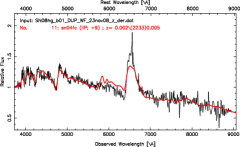
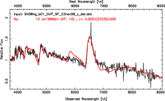
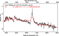
Figure 143.— Best spectral matching of SN 2008hg using SNID. The plots show SN 2008hg compared with SN 2004et, SN 2006bp, SN 2004fc, SN 1999em, and 2006iw at 17, 13, 9, 10, amd 11 days from explosion.

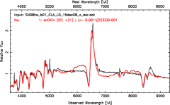
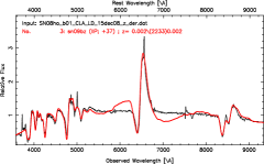
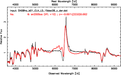
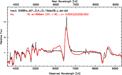
Figure 144.— Best spectral matching of SN 2008ho using SNID. The plots show SN 2008ho compared with SN 2004fx, SN 2009bz, SN 2005cs, and SN 1999em at 31, 37, 16, and 26 days from explosion.

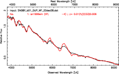
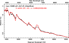
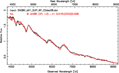
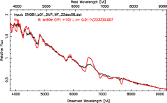
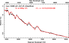
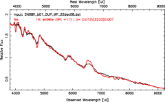
Figure 145.— Best spectral matching of SN 2008if using SNID. The plots show SN 2008if compared with SN 1999em, SN 2004fc, SN 2008il, SN 1990E, SN 1999gi, and SN 2006iw at 6, 9, 3, 10, 8, and 11 days from explosion.

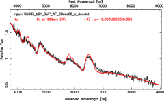
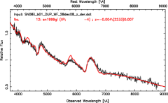
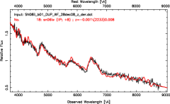
Figure 146.— Best spectral matching of SN 2008il using SNID. The plots show SN 2008il compared with SN 1999em, SN 1999gi, and SN 2006iw at 6, 8, and 8 days from explosion.

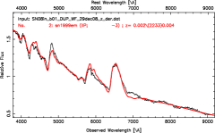
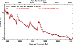
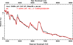
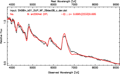
Figure 147.— Best spectral matching of SN 2008in using SNID. The plots show SN 2008in compared with SN 1999em, SN 2005cs, SN 2004fc, and SN 2004et at 7, 6, 9, and 13 days from explosion.

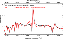
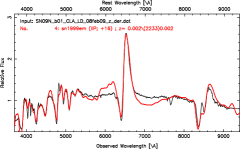
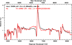
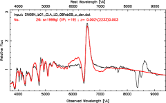
Figure 148.— Best spectral matching of SN 2009N using SNID. The plots show SN 2009N compared with SN 2005cs, SN 1999em, SN 1999br, and SN 1999gi at 22, 16, 25, 31 days from explosion.

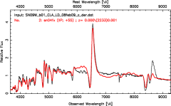
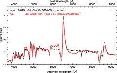
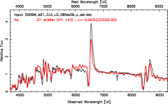
Figure 149.— Best spectral matching of SN 2009W using SNID. The plots show SN 2009W compared with SN 2004fx, SN 2008il, and SN 1999br at 55, 63, and 43 days from explosion.

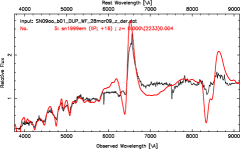
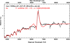
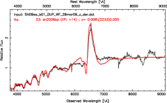
Figure 150.— Best spectral matching of SN 2009ao using SNID. The plots show SN 2009ao compared with SN 1999em, SN 2004et, and SN 2006bp at 26, 22, and 24 days from explosion.

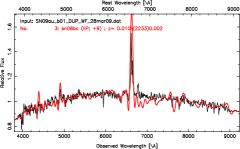
Figure 151.— Best spectral matching of SN 2009au using SNID. The plots show SN 2009au compared with SN 2006bc at 9 days from explosion.

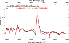
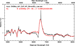
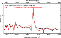
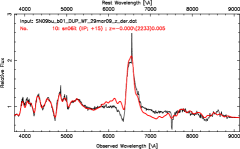
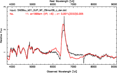
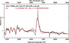
Figure 152.— Best spectral matching of SN 2009bu using SNID. The plots show SN 2009bu compared with SN 2003bn, SN 2006bp, SN 2005dz, SN 2006it, SN 1999em, and SN 2004et at 16, 17, 20, 15, 16, and 22 days from explosion.

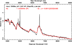
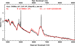
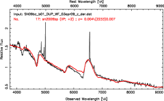
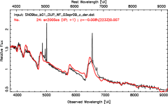
Figure 153.— Best spectral matching of SN 2009bz using SNID. The plots show SN 2009bz compared with SN 2004et, SN 1999em, SN 2006bp, and SN 2005cs at 13, 8, 11, and 7 days from explosion.

References

- Allington-Smith et al. (1994) Allington-Smith, J., Breare, M., Ellis, R., et al. 1994, PASP, 106, 983
- Anderson et al. (2014a) Anderson, J. P., Dessart, L., Gutierrez, C. P., et al. 2014a, MNRAS, 441, 671
- Anderson et al. (2014b) Anderson, J. P., et al. 2014b, ApJ, 786, 67
- Anderson et al. (2016) Anderson, J. P., Gutiérrez, C. P., Dessart, L., et al. 2016, A&A, 589, A110
- Arcavi et al. (2010) Arcavi, I., Gal-Yam, A., Kasliwal, M. M., et al. 2010, ApJ, 721, 777
- Barbon et al. (1999) Barbon, R., Buondí, V., Cappellaro, E., & Turatto, M. 1999, A&AS, 139, 531
- Barbon et al. (1979) Barbon, R., Ciatti, F., & Rosino, L. 1979, A&A, 72, 287
- Baron et al. (2000) Baron, E., Branch, D., Hauschildt, P. H., et al. 2000, ApJ, 545, 444
- Blanco et al. (1987) Blanco, V. M., Gregory, B., Hamuy, M., et al. 1987, ApJ, 320, 589
- Blondin & Tonry (2007) Blondin, S., & Tonry, J. L. 2007, ApJ, 666, 1024
- Bose et al. (2013) Bose, S., Kumar, B., Sutaria, F., et al. 2013, MNRAS, 433, 1871
- Branch et al. (1981) Branch, D., Falk, S. W., Uomoto, A. K., et al. 1981, ApJ, 244, 780
- Buta (1982) Buta, R. J. 1982, PASP, 94, 578
- Buzzoni et al. (1984) Buzzoni, B., Delabre, B., Dekker, H., et al. 1984, The Messenger, 38, 9
- Cappellaro et al. (1995) Cappellaro, E., Danziger, I. J., della Valle, M., Gouiffes, C., & Turatto, M. 1995, A&A, 293, 723
- Chugai et al. (2007) Chugai, N. N., Chevalier, R. A., & Utrobin, V. P. 2007, ApJ, 662, 1136
- Contreras et al. (2010) Contreras, C., Hamuy, M., Phillips, M. M., et al. 2010, AJ, 139, 519
- Dall’Ora et al. (2014) Dall’Ora, M., Botticella, M. T., Pumo, M. L., et al. 2014, ApJ, 787, 139
- Dekker et al. (1986) Dekker, H., Delabre, B., & Dodorico, S. 1986, in Proc. SPIE, Vol. 627, Instrumentation in astronomy VI, ed. D. L. Crawford, 339–348
- Dessart & Hillier (2005) Dessart, L., & Hillier, D. J. 2005, A&A, 437, 667
- Dessart & Hillier (2006) —. 2006, A&A, 447, 691
- Dessart & Hillier (2008) —. 2008, MNRAS, 383, 57
- Dessart & Hillier (2010) —. 2010, MNRAS, 405, 2141
- Dessart & Hillier (2011) —. 2011, MNRAS, 410, 1739
- Dessart et al. (2013) Dessart, L., Hillier, D. J., Waldman, R., & Livne, E. 2013, MNRAS, 433, 1745
- Dessart et al. (2008) Dessart, L., Blondin, S., Brown, P. J., et al. 2008, ApJ, 675, 644
- Dressler et al. (2011) Dressler, A., Bigelow, B., Hare, T., et al. 2011, PASP, 123, 288
- Dwek (1983) Dwek, E. 1983, ApJ, 274, 175
- Fabbri et al. (2011) Fabbri, J., Otsuka, M., Barlow, M. J., et al. 2011, MNRAS, 418, 1285
- Faran et al. (2014a) Faran, T., Poznanski, D., Filippenko, A. V., et al. 2014a, MNRAS, 445, 554
- Faran et al. (2014b) —. 2014b, MNRAS, 442, 844
- Fesen et al. (1999) Fesen, R. A., Gerardy, C. L., Filippenko, A. V., et al. 1999, AJ, 117, 725
- Filippenko et al. (1993) Filippenko, A. V., Matheson, T., & Ho, L. C. 1993, ApJ, 415, L103
- Folatelli et al. (2010) Folatelli, G., Phillips, M. M., Burns, C. R., et al. 2010, AJ, 139, 120
- Folatelli et al. (2013) Folatelli, G., Morrell, N., Phillips, M. M., et al. 2013, ApJ, 773, 53
- Fransson & Chevalier (1987) Fransson, C., & Chevalier, R. A. 1987, ApJ, 322, L15
- Galbany et al. (2016) Galbany, L., Hamuy, M., Phillips, M. M., et al. 2016, AJ, 151, 33
- Gutiérrez et al. (2014) Gutiérrez, C. P., et al. 2014, ApJ, 786, L15
- Hamuy (2003) Hamuy, M. 2003, ApJ, 582, 905
- Hamuy et al. (1996) Hamuy, M., Phillips, M. M., Suntzeff, N. B., et al. 1996, AJ, 112, 2438
- Hamuy & Pinto (2002) Hamuy, M., & Pinto, P. A. 2002, ApJ, 566, L63
- Hamuy et al. (1988) Hamuy, M., Suntzeff, N. B., Gonzalez, R., & Martin, G. 1988, AJ, 95, 63
- Hamuy et al. (1993) Hamuy, M., Maza, J., Phillips, M. M., et al. 1993, AJ, 106, 2392
- Hamuy et al. (2001) Hamuy, M., Pinto, P. A., Maza, J., et al. 2001, ApJ, 558, 615
- Hamuy et al. (2006) Hamuy, M., Folatelli, G., Morrell, N. I., et al. 2006, PASP, 118, 2
- Hamuy (2001) Hamuy, M. A. 2001, PhD thesis, The University of Arizona
- Harutyunyan et al. (2008) Harutyunyan, A. H., et al. 2008, A&A, 488, 383
- Howell et al. (2005) Howell, D. A., et al. 2005, ApJ, 634, 1190
- Immler et al. (2005) Immler, S., Fesen, R. A., Van Dyk, S. D., et al. 2005, ApJ, 632, 283
- Inserra et al. (2011) Inserra, C., Turatto, M., Pastorello, A., et al. 2011, MNRAS, 417, 261
- Inserra et al. (2012) —. 2012, MNRAS, 422, 1122
- Inserra et al. (2013) Inserra, C., Pastorello, A., Turatto, M., et al. 2013, A&A, 555, A142
- Jerkstrand et al. (2012) Jerkstrand, A., Fransson, C., Maguire, K., et al. 2012, A&A, 546, A28
- Jerkstrand et al. (2014) Jerkstrand, A., Smartt, S. J., Fraser, M., et al. 2014, MNRAS, 439, 3694
- Jones et al. (2009) Jones, M. I., Hamuy, M., Lira, P., et al. 2009, ApJ, 696, 1176
- Kotak et al. (2009) Kotak, R., Meikle, W. P. S., Farrah, D., et al. 2009, ApJ, 704, 306
- Leonard et al. (2002a) Leonard, D. C., Filippenko, A. V., Li, W., et al. 2002a, AJ, 124, 2490
- Leonard et al. (2002b) Leonard, D. C., Filippenko, A. V., Gates, E. L., et al. 2002b, PASP, 114, 35
- Li et al. (2005) Li, W., Van Dyk, S. D., Filippenko, A. V., & Cuillandre, J.-C. 2005, PASP, 117, 121
- Lisakov et al. (2017) Lisakov, S. M., Dessart, L., Hillier, D. J., Waldman, R., & Livne, E. 2017, MNRAS, 466, 34
- Maguire et al. (2010) Maguire, K., Di Carlo, E., Smartt, S. J., et al. 2010, MNRAS, 404, 981
- Marino et al. (2013) Marino, R. A., Rosales-Ortega, F. F., Sánchez, S. F., et al. 2013, A&A, 559, A114
- Maund & Smartt (2005) Maund, J. R., & Smartt, S. J. 2005, MNRAS, 360, 288
- Menzies et al. (1987) Menzies, J. W., Catchpole, R. M., van Vuuren, G., et al. 1987, MNRAS, 227, 39P
- Minkowski (1941) Minkowski, R. 1941, PASP, 53, 224
- Misra et al. (2007) Misra, K., et al. 2007, MNRAS, 381, 280
- Müller et al. (2017) Müller, T., Prieto, J. L., Pejcha, O., & Clocchiatti, A. 2017, ApJ, 841, 127
- Olivares (2008) Olivares, F. 2008, ArXiv e-prints
- Pastorello et al. (2004) Pastorello, A., Zampieri, L., Turatto, M., et al. 2004, MNRAS, 347, 74
- Pastorello et al. (2006) Pastorello, A., Sauer, D., Taubenberger, S., et al. 2006, MNRAS, 370, 1752
- Pastorello et al. (2009) Pastorello, A., Valenti, S., Zampieri, L., et al. 2009, MNRAS, 394, 2266
- Patat et al. (1994) Patat, F., Barbon, R., Cappellaro, E., & Turatto, M. 1994, A&A, 282, 731
- Pejcha & Prieto (2015a) Pejcha, O., & Prieto, J. L. 2015a, ApJ, 799, 215
- Pejcha & Prieto (2015b) —. 2015b, ApJ, 806, 225
- Phillips et al. (1988) Phillips, M. M., Heathcote, S. R., Hamuy, M., & Navarrete, M. 1988, AJ, 95, 1087
- Pooley et al. (2002) Pooley, D., Lewin, W. H. G., Fox, D. W., et al. 2002, ApJ, 572, 932
- Roy et al. (2011) Roy, R., Kumar, B., Benetti, S., et al. 2011, ApJ, 736, 76
- Sahu et al. (2006) Sahu, D. K., Anupama, G. C., Srividya, S., & Muneer, S. 2006, MNRAS, 372, 1315
- Sanders et al. (2015) Sanders, N. E., Soderberg, A. M., Gezari, S., et al. 2015, ApJ, 799, 208
- Schlafly & Finkbeiner (2011) Schlafly, E. F., & Finkbeiner, D. P. 2011, ApJ, 737, 103
- Schlegel (1990) Schlegel, E. M. 1990, MNRAS, 244, 269
- Schmidt et al. (1993) Schmidt, B. P., Kirshner, R. P., Schild, R., et al. 1993, AJ, 105, 2236
- Smartt (2015) Smartt, S. J. 2015, Publications of the Astronomical Society of Australia, 32, e016
- Smartt et al. (2009) Smartt, S. J., Eldridge, J. J., Crockett, R. M., & Maund, J. R. 2009, MNRAS, 395, 1409
- Smartt et al. (2004) Smartt, S. J., Maund, J. R., Hendry, M. A., et al. 2004, Science, 303, 499
- Spiro et al. (2014) Spiro, S., Pastorello, A., Pumo, M. L., et al. 2014, ArXiv e-prints
- Stritzinger et al. (2011) Stritzinger, M. D., et al. 2011, AJ, 142, 156
- Stritzinger et al. (2017) Stritzinger, M. D., Anderson, J. P., Contreras, C., et al. 2017, ArXiv e-prints
- Suntzeff et al. (1988) Suntzeff, N. B., Hamuy, M., Martin, G., Gomez, A., & Gonzalez, R. 1988, AJ, 96, 1864
- Taddia et al. (2012) Taddia, F., Stritzinger, M. D., Sollerman, J., et al. 2012, A&A, 537, A140
- Taddia et al. (2013) Taddia, F., et al. 2013, A&A, 555, A10
- Taddia et al. (2017) Taddia, F., Stritzinger, M. D., Bersten, M., et al. 2017, ArXiv e-prints
- Tomasella et al. (2013) Tomasella, L., Cappellaro, E., Fraser, M., et al. 2013, MNRAS, 434, 1636
- Turatto et al. (1993) Turatto, M., Cappellaro, E., Benetti, S., & Danziger, I. J. 1993, MNRAS, 265, 471
- Valenti et al. (2013) Valenti, S., et al. 2013, ArXiv e-prints
- Valenti et al. (2016) Valenti, S., Howell, D. A., Stritzinger, M. D., et al. 2016, MNRAS, 459, 3939
- Van Dyk et al. (2003) Van Dyk, S. D., Li, W., & Filippenko, A. V. 2003, PASP, 115, 1289
- Wood-Vasey et al. (2004) Wood-Vasey, W. M., Aldering, G., Lee, B. C., et al. 2004, New Astronomy Reviews, 48, 637