A classifier for gravitational-wave inspiral signals in non-ideal single-detector data

Abstract

We describe a multivariate classifier for candidate events in a templated search for gravitational-wave (GW) inspiral signals from neutron-star–black-hole (NS-BH) binaries, in data from ground-based detectors where sensitivity is limited by non-Gaussian noise transients. The standard signal-to-noise ratio (SNR) and chi-squared test for inspiral searches use only properties of a single matched filter at the time of an event; instead, we propose a classifier using features derived from a bank of inspiral templates around the time of each event, and also from a search using approximate sine-Gaussian templates. The classifier thus extracts additional information from strain data to discriminate inspiral signals from noise transients. We evaluate a Random Forest classifier on a set of single-detector events obtained from realistic simulated advanced LIGO data, using simulated NS-BH signals added to the data. The new classifier detects a factor of 1.5 – 2 more signals at low false positive rates as compared to the standard ‘re-weighted SNR’ statistic, and does not require the chi-squared test to be computed. Conversely, if only the SNR and chi-squared values of single-detector events are available, Random Forest classification performs nearly identically to the re-weighted SNR.

I Introduction

I.1 Motivation

The epoch of gravitational wave astronomy has begun with the unambiguous detection of GW signals from massive merging binary black hole (BBH) systems Abbott et al. (2016a, b, c, d, e, f, 2017) in data from the Advanced LIGO interferometers Abbott et al. (2016g). Already, though, the non-detection of binary neutron-star (BNS) and neutron star-black hole (NS-BH) binaries in the first Advanced LIGO observing run Abbott et al. (2016h) provides motivation to further develop search methods for coalescing binaries (CBC) in order to fully realize the science potential of the Advanced detector network Aasi et al. (2015a); Acernese et al. (2015). Moreover, since it appears that elucidating the origin of merging BBH systems may require some tens of detections (see e.g. Stevenson et al. (2017)), it is also desirable to increase the sensitivity of searches to relatively weak CBC signals, which should be more numerous than high-SNR detections.

Consider a signal comparable to the candidate event LVT151012, which has a network SNR of $\sim 9.7$, consistent with a massive BBH merger at redshift $\sim 0.2$ if astrophysical, but is assigned a false alarm rate of $0.4$ per year in the advanced LIGO-Virgo search pipeline of Abbott et al. (2016b, f); Usman et al. (2016). (This false alarm rate is the expected number of noise events with a higher ranking than LVT151012 in the given search pipeline, per year of data searched.) We could not confidently rule out that an event with comparable SNR was due to noise with current methods. Noise events louder than such relatively weak signals are still dominated by transient detector artefacts (‘glitches’), which are generally suppressed by the standard chi-squared test Allen (2005); Allen et al. (2012) but not eliminated. If new methods are able to further reduce the contribution of non-Gaussian artefacts to the noise background, the search sensitivity to weak signals could be significantly increased, as an improved pipeline would assign such events lower false alarm rates relative to current methods, corresponding to a higher probability of astrophysical origin via the analysis of Abbott et al. (2016i, j).

I.2 Detection statistics and followup for inspiral events

Searches for GW from inspiraling compact binary sources in data from ground-based detectors Babak et al. (2013a); Abbott et al. (2009a, b); Abadie et al. (2010a, 2012) have so far relied on empirical methods to suppress the effects of non-Gaussian noise transients (‘glitches’) Blackburn et al. (2008); Slutsky et al. (2010); Aasi et al. (2015b). These transients give rise to a background distribution of ‘triggers’ (maxima of the matched filter SNR time series Allen et al. (2012)) with SNRs up to $10^{2}$–$10^{3}$, whereas Gaussian noise would, for typical search parameters, produce a maximum network SNR of order 10 or less. Without any steps to exclude or down-rank very high noise SNRs, the search sensitivity for astrophysical signals would be reduced by orders of magnitude Babak et al. (2013a).

Various signal consistency tests for loud triggers in binary inspiral searches have been considered Allen (2005); Rodriguez (2007); Babak et al. (2005); Hanna (2008); Harry and Fairhurst (2011); Messick et al. (2017); the time-frequency $\chi^{2}$ test described in Allen (2005) has been widely employed, due to its relative simplicity and effectiveness over a range of different epochs of data and signal parameters. In ‘all-sky’ searches (those without a restriction on the times and sky directions searched) candidate events have been ranked by a simple algebraic function of the matched filter SNR $\rho$ and $\chi^{2}$ of single-detector triggers (‘effective SNR’ or ‘re-weighted SNR’) Babak et al. (2013a); Abadie et al. (2012) which pass a consistency test between their arrival time and mass parameters Robinson et al. (2008).

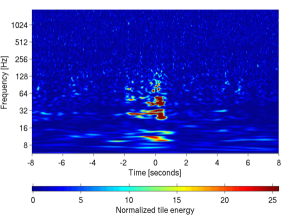
In principle the loudest search events, i.e. those with highest combined re-weighted SNR $\hat{\rho}$, are the most likely to indicate GW signals Babak et al. (2013a); Abadie et al. (2012). Conversely, the loudest events generated by unphysical relative time-shifts of detectors at different locations, used to estimate the noise background of the search, are those which restrict the sensitivity of the search at low false alarm rate. However, when examining the properties of these loudest events in detail Gouaty (2008), we often find that even triggers with high $\hat{\rho}$ appear to be caused by loud glitches, or occur in times of sub-optimal data quality as shown by the presence of excess noise over periods of  seconds. Such excess noise can be diagnosed by the presence of many high-energy tiles when decomposing the strain data in an approximate sine-Gaussian basis Chatterji (1995); a ‘Q-scan’ or ‘Omega scan’ diagnostic output for a few seconds of poor quality data from the LIGO S6 science run is shown in Fig. 1. In contrast, an inspiraling binary signal in Gaussian noise viewed in this basis would either have no loud tiles at all, or if the signal was strong, the loud tiles would trace a clear ‘chirp’ trajectory in time and frequency, as in Fig. 1 of Abbott et al. (2016a) and (for simulated signals) in Fig. 6 of Gouaty (2008) and the LIGO-Virgo S6/VSR3 blind injection data release Collaboration and Collaboration (2011).

Figure 1: Diagnostic whitened spectrogram (‘Omegagram’) from a decomposition of LIGO strain data in an approximate sine-Gaussian basis, showing excess noise power (‘tile energy’) over for a few seconds of searched data. Such non-Gaussian noise gives rise to some of the highest-ranked events in a matched filter search for inspiral signals where the well-known time-frequency $\chi^{2}$ test is employed.

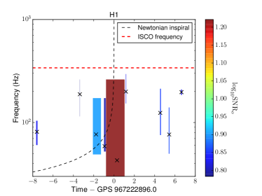
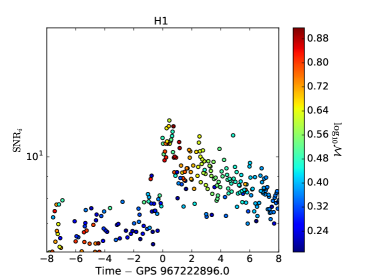
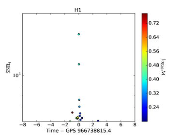
Furthermore, when examining the triggers from the inspiral search around the time of a candidate (plots known as ‘mini-followup’), we often find that the loudest events show large numbers of high-SNR triggers spread over several seconds, whereas for an inspiral signal in Gaussian noise we expect a small number of high-SNR triggers localized within a fraction of a second of the loud event and with similar chirp mass, defined as

$$\mathcal{M}=(m_{1}m_{2})^{3/5}(m_{1}+m_{2})^{-1/5},$$ (1)

where $m_{1,2}$ are the binary component masses. See the right-hand plots in Figures 3 and 3 respectively for examples of ‘glitchy’ vs. ’clean’ sets of triggers around a loud event. These two plots can easily be distinguished although the highest-SNR trigger has similar properties in both. Thus, the strain data around the time of a noise trigger of high $\hat{\rho}$ will likely contain more information than the $\chi^{2}$ statistic, which uses only the samples of the matched filter integral for that trigger, divided into frequency bins Allen (2005).

I.3 Outline of classifier method

Our objective here is to identify additional information available in the strain data and employ it effectively in distinguishing triggers due to binary inspiral-merger signals from those caused by noise transients. To do so we will construct a ranking statistic that uses several independent, or partially correlated, pieces of information (‘features’) extracted from the data around each inspiral search trigger. Some of these features consist of information already available in the output of the inspiral matched filter search, namely the coalescence times, SNRs and parameters of other triggers close to the event under consideration.

Our classification information also includes the output of another analysis algorithm, omicron Robinet (2016), which responds to transient signals or artefacts in a very different way from the inspiral matched filter search. Omicron is an adaptation of the Q-pipeline and Omega search methods Chatterji (1995); Abbott et al. (2009c) which aim to detect transient events with excess power localized in time and frequency, without placing strong constraints on the morphology of such events. Omega/omicron have also been applied to single-interferometer data for characterization of non-Gaussian noise transients in LIGO and Virgo data Aasi et al. (2015b, 2012); our use of omicron has a similar motivation, as we are seeking to down-rank times where strain data contains high-amplitude noise artifacts. A set of omicron triggers may contain information on such noise events which is at least partly independent of that contained in inspiral matched filter triggers.

To combine features derived from omicron triggers with those from the inspiral search triggers, we implement a Random Forest multivariate classifier Ran trained on both noise triggers derived from realistic simulated early Advanced LIGO data, and on simulated neutron-star black-hole (NS-BH) binary signals added to such data. We then use independent trigger samples to evaluate how efficiently the classifier sorts noise from signal events.

I.4 Relation to previous work

Multivariate classification methods to separate transient GW signals from non-Gaussian artefacts have been proposed and implemented in the context of templated searches for inspiral-merger-ringdown (IMR) signals from stellar-mass or intermediate mass binary black holes Baker et al. (2015); Hodge (2014), and in a search for weakly-modelled GW burst signals associated with external high-energy electromagnetic triggers Adams et al. (2013). The possible improvement in efficiency of a coherent templated search for inspiral GW signals associated with gamma-ray bursts (GRB) Harry and Fairhurst (2011) due to use of a neural network was also investigated in Kim et al. (2015). Our work differs from these methods in two main respects. First, in contrast to previous work which uses properties of events derived from multi-detector analysis, we show that multivariate classification can be effective even using only the data stream from a single detector. Our approach may then be useful to ‘modularize’ the classification problem for a multi-detector network, splitting the calculation into parts which depend on the noise properties in each separate detector and parts which depend on the joint properties of an event compared in several detectors.

Second, we build our classification information from the outputs of two entirely independent analyses applied to a given data stream, effectively viewing the data in two different ways, which allows us to extract information which would not be available when using the output of a single search pipeline alone. In the case we consider, the omicron (burst) analysis acts as a diagnostic for non-Gaussian noise similar to a followup by visual inspection of the data. We also use information from times surrounding a candidate trigger, rather than only at the peak of the likelihood; this information helps to diagnose the state of the detector, uncovering times of worse quality data where frequent glitches occur.

Overview of the paper

We will proceed in Section II by setting out the problem to be addressed in classifying inspiral search events (triggers) and defining a figure of merit for the outcome of the classification. We give a brief introduction to the Random Forest method of multivariate classification in Section III, then describe its application to the case of a templated search for inspiral GW signals in Section IV. The tuning of classifier parameters and the results of evaluating the classifier on simulated non-ideal early Advanced era detector data are given in Section V, with Section VI giving conclusions and discussion of possible further steps.

II Statistics of event classification

The detection of transient gravitational-wave signals in data from interferometric detectors such as Advanced LIGO and Virgo Aasi et al. (2015a); Acernese et al. (2015) is a statistical classification problem. Given the expected rates of occurrence of source events Abadie et al. (2010b), most time samples in the detector outputs will contain either no signal, or a signal that is so weak as to be indistinguishable from zero by any means in the presence of detector noise. The task is then to sort the few time samples that are likely to contain an identifiable signal, and thus contain information on the nature of a GW source, from the overwhelming majority of noise-only samples.

This sorting is done by considering short time periods (such that each is extremely unlikely to contain more than $1$ signal) and assigning each period labelled by $i$ a real number $\Lambda_{i}$, where large $\Lambda$ indicates a greater likelihood that a signal is present and small $\Lambda$ indicates a smaller likelihood of signal, i.e. a greater likelihood that time $i$ contains only noise. Times when $\Lambda$ exceeds a threshold $\Lambda_{t}$ are considered as candidate signals.

Due to the presence of random (unpredictable) noise in the detector outputs, this classification can never be perfectly reliable. Even with a high threshold $\Lambda_{t}$, the false positive rate (FPR) $p_{f}(\Lambda_{t})\equiv p(\Lambda_{i}>\Lambda_{t}|N)$, where $N$ indicates the hypothesis of data containing noise only, can never be reduced to zero. Conversely, raising the threshold will cause the detection probability $p_{d}(\Lambda_{t})\equiv p(\Lambda_{i}>\Lambda_{t}|S)$ to decrease, where $S$ indicates the hypothesis of data containing noise plus a signal of non-negligible amplitude. In addition, if the signals have a distribution of amplitudes, the weaker signals are less likely to produce a $\Lambda$ value above any specific threshold. A classification method mapping the data at time $i$ to a $\Lambda_{i}$ value is optimized by maximizing $p_{d}$, marginalized over a given distribution of signal parameters Searle (2008), at fixed $p_{f}$. In practice the threshold $\Lambda_{t}$ may be adjusted to obtain a desired $p_{f}$ value.

An optimal search statistic will then be given by the likelihood ratio $\Lambda_{i,{\rm opt}}\equiv p(d_{i}|S)/p(d_{i}|N)$: in words, the relative likelihood that the data at time $i$ is caused by a signal plus noise, versus by noise only. Our task is then, if possible, to evaluate $\Lambda_{i,{\rm opt}}$ for the actual noise seen at detector outputs and for the desired signals; if this is not possible from first principles, then to obtain a good approximation to it.

The matched filter is an optimal method for a signal of known form in stationary noise, and may straightforwardly be extended to post-Newtonian signal waveforms from quasi-circular non-precessing binary systems for which the coalescence time, phase and amplitude are unknown Sathyaprakash and Dhurandhar (1991); Finn and Chernoff (1993); Allen et al. (2012). Briefly, each signal template is correlated with the strain data in Fourier domain, weighting by the inverse of the detector noise power spectrum (power spectral density, PSD). The resulting time series, normalized such that the template’s correlation with itself is unity, is maximized over complex phase to obtain a real SNR $\rho(t)$, which is then maximized over time (over periods of typically a few seconds) to obtain triggers. The trigger SNR $\rho_{i}$ is, to a good approximation, a monotonic function of $\Lambda_{i}$, and is thus suitable as a detection statistic.

The above is only true if the noise is indeed Gaussian and stationary; however, real detector strain shows a large number of transients well localized in time – “glitches” – caused by more or less well-understood instrumental or environmental effects; see e.g. Abbott et al. (2004); Blackburn et al. (2008); Aasi et al. (2015b, 2012). Although many such transient artefacts may be readily identified and removed from searches Slutsky et al. (2010), large numbers remain unexplained, particularly with relatively low amplitude (SNRs of order 10-20; though such values are still strongly inconsistent with Gaussian noise). The presence of non-stationary transients invalidates the matched filter SNR as a detection statistic and ranking events by $\rho_{i}$ then leads to a vast loss of sensitivity to signals compared to a search in Gaussian noise with comparable PSD Usman et al. (2016).

Hence a different strategy must be adopted. Searches for inspiraling binary signals in LIGO-Virgo data have implicitly assumed that the majority of time samples are well modelled by stationary, Gaussian noise, with a small number of times affected by glitches. This motivates calculating additional quantities besides $\rho$ which will indicate the presence of a glitch, then vetoing (removing) or down-ranking affected times. A widely used test is the time-frequency chi-squared Allen (2005) which splits the template waveform into several frequency bands and checks whether the matched filter output for each one at the time of the supposed signal is consistent with expected amplitude and phase. High-amplitude glitches have large $\chi^{2}$ values relative to the expectation in Gaussian noise, while signals which are well matched to a given template have small $\chi^{2}$ (approximately $1$ per degree of freedom). Recent searches have used the “re-weighted SNR” $\hat{\rho}(\rho,\chi^{2})$ of single-detector triggers as a ranking statistic Abadie et al. (2012); Babak et al. (2013b); Abbott et al. (2016b); Usman et al. (2016):

$$\hat{\rho}=\begin{cases}\rho&\textrm{for }\chi^{2}\leq n_{\rm dof}\\ \rho\left[\left(1+(\frac{\chi^{2}}{n_{\rm dof}})^{3}\right)/2\right]^{-\frac{1}{6}}&\textrm{for }\chi^{2}>n_{\rm dof},\end{cases}$$ (2)

where $n_{\mathrm{dof}}=2p-2$ is the number of degrees of freedom of the $\chi^{2}$ test with $p$ frequency bands. (For multi-detector events, the ranking statistic is taken to be the quadrature sum of $\hat{\rho}$ values over detectors.)

We would like to generalize such a ranking statistic to a function of several pieces of information available for each binary merger search trigger, called ‘features’. For instance, each trigger has an SNR value, a template chirp mass $\mathcal{M}$, etc.. We notate each trigger’s features as a $p$-dimensional vector ${\bf x}$; triggers resulting from detector noise are written as ${\bf x}_{n}$, those arising from (simulated or real) signal added to noise as ${\bf x}_{s}$. We write the total number of noise and signal triggers as $N_{n}$ and $N_{s}$, respectively.

Given a classification method which assigns a trigger with features ${\bf x}$ a likelihood of belonging to either ${\bf x}_{n}$ or ${\bf x}_{s}$, we require a method to assess the performance of the classifier. Typically, a classifier needs to “train” itself on a set of candidate events where the status of each ${\bf x}$ as noise or signal is already known. Given the low rate of detected GW in existing data and the trigger generation threshold adopted in this analysis, the great majority of triggers will be due to noise. To train a classifier we also require a large number of simulated GW signals, typically via injecting (adding) the signal strain to the detector data to produce a set of candidate events.

In principle, one could train the classifier on the entire set of simulated triggers at hand, and test it on the same set of triggers. This method however is susceptible to overfitting, making it difficult to trust the classifier’s predictions on trigger sets it has not trained on. In order to circumvent this problem, cross-validation is employed: a portion of the trigger set is kept aside for testing, while the remaining triggers are used for training. A more sophisticated version, stratified K-fold cross validation, splits the data into $K$ partitions or “folds”, where $K$ is an integer greater than unity. Stratification ensures that each partition is well balanced, and not skewed in favour of one or other class. The classifier then trains itself on $K-1$ folds, the remaining fold having been kept aside for testing. This process is repeated $K$ times, with each repetition using a different fold for testing and correspondingly a different set of folds for training.

There are two kinds of classification models: discrete and probabilistic. The discrete classifier directly labels a candidate event ${\bf x}$ in a test set as either ${\bf x}_{n}$ or ${\bf x}_{s}$. The probabilistic classifier assigns a score $\hat{p}$ to a trigger, the score being a continuous variable. Typically, though not necessarily, $\hat{p}$ is an estimate of the probability that a trigger is a signal event. The Random Forest multivariate classifier used in this project outputs such an estimate, which may then be used to predict whether the trigger is associated with a noise or signal event by setting a threshold value $\hat{p}_{t}$ for the classifier score.

For each prediction of a trigger’s category, there are four possible cases. These may be summarized by a so-called confusion matrix, with the four elements “True Positive”, “False Positive”, “False Dismissal”, “True Dismissal”. True Positive (True Dismissal) corresponds to a signal (noise) trigger accurately labelled as ${\bf x}_{s}$ (${\bf x}_{n}$). False Positive (False Dismissal) corresponds to a noise (signal) trigger wrongly labelled as ${\bf x}_{s}$ (${\bf x}_{n}$). If $N_{\rm TP}$ and $N_{\rm FP}$ are the numbers of True Positives and False Positives evaluated from the output of the classifier at a specific threshold $\hat{p}_{t}$, then the classical Detection Probability (DP) and False Positive Rate (notated as $\alpha$) are estimated as

$$DP=\frac{N_{\rm TP}}{N_{s}},$$ (3)

$$\alpha=\frac{N_{\rm FP}}{N_{n}}.$$ (4)

These quantities summarize the performance of the classifier, and can be represented visually via the “receiver operating characteristic” (ROC) graph.

The detection probability and false positive rate computed from the output of a probabilistic classifier, like the one employed in this project, are a function of the score threshold used to label triggers. By varying the threshold value from $0$ to $1$, an ROC curve may be created. Here we use the classifier scores assigned to simulated signals as thresholds for plotting the ROC. The false positive rate associated with a signal trigger $\alpha_{s}$ is computed by counting the number of noise triggers whose scores $\hat{p}_{n}^{i}$ are greater than the score of the signal trigger $\hat{p}_{s}$:

$$\alpha_{s}=\frac{1}{N_{n}}\sum^{N_{n}}_{i=1}\Theta(\hat{p}^{i}_{n}-\hat{p}_{s}).$$ (5)

For reasons of computational expense, the amplitude distribution of simulated signals used in this study is different from the astrophysical $\rho^{-4}$ distribution expected for merging binaries uniformly distributed over space. Our set of simulated mergers is, instead, evenly distributed in distance from the detector, leading to an expected $\rho^{-2}$ distribution of signals. Therefore the detection probability for a given threshold $\hat{p}_{t}$ is not directly proportional to the number of simulated signals with higher scores; instead, we compute a figure of merit proportional to the expected number of detections, $N_{d}$, by performing a weighted sum of signal triggers. To compensate for the non-astrophysical distribution of signal amplitudes we use a weighting inversely proportional to the square of the trigger SNR $\rho_{s}^{j}$,

$$w_{\mathrm{ROC}}^{j}=\left(\frac{8}{\rho_{s}^{j}}\right)^{2}.$$ (6)

Our estimate of the relative number of detections $N_{d}$ at a threshold $\hat{p}_{s}$ is the sum of weights $w_{\mathrm{ROC}}^{j}$ over simulated signal triggers $j$ with scores $\hat{p}_{s}^{j}$ greater than $\hat{p}_{s}$:

$$N_{d}(\hat{p}_{s})=\sum_{j=1}^{N_{s}}w_{\mathrm{ROC}}^{j}\Theta(\hat{p}_{s}^{j}-\hat{p}_{s}).$$ (7)

Every point ($\alpha_{s}$, $N_{d}$) on the ROC plot then corresponds to classification using the score $\hat{p}_{s}$ of a given signal trigger as a threshold. We may also compute the figure of merit for a predefined set of $\alpha$ values: $N_{d}$ evaluated at a chosen $\alpha$ is the sum of weights $w_{\mathrm{ROC}}^{j}$ for signal triggers whose false positive rates $\alpha_{s}^{j}$ evaluated via Eq. (5) are less than or equal to the chosen $\alpha$:

$$N_{d}(\alpha)=\sum_{j=1}^{N_{s}}w_{\mathrm{ROC}}^{j}\Theta(\alpha-\alpha_{s}^{j}).$$ (8)

Note that $N_{d}$ is only defined up to an arbitrary multiplicative constant; one cannot use it to predict the absolute number or rate of signal detections, only to compare the relative number of detections between different classifiers, i.e. different methods of assigning scores $\hat{p}$ to triggers ${\bf x}$.

III Random Forest as a multivariate classifier

The Random Forest (RF) is an ensemble classifier consisting of a collection of random decision trees Ran . The RF algorithm employed in this project uses a particular kind of decision tree known as a classification tree, which, when trained, predicts the probability of class membership of test data points. A classification tree has a structure similar to a flowchart, made up of a root node, internal nodes, branches and leaf nodes. Each internal node is connected to a parent node and two child/daughter nodes via branches, starting with the root node (with no parent) and ending at leaf nodes (with no children). During training, each node splits the training data set into two sections and sends them along branches to daughter nodes. The branch that a data point will follow depends on the splitting condition imposed at the parent node.

In principle, each point in a $p$-dimensional feature space provides $p$ possible splitting criteria; if this space contains an infinite number of such points, these would correspond to an infinite number of ways in which the training data set can be segregated. In practice, not all of those splits will result in unique two-way divisions of the data set. Typically, one considers only those $n$ points in feature space that are occupied by the $n$ training data points themselves, and chooses the splitting condition from $n\times p$ possible attribute values that minimizes the mixing of classes at the daughter nodes. We use “Gini Impurity” ($I_{G}$) as a measure of this mixing of classes. The Gini Impurity at a node that has data points from $m$ classes is computed using the formula:

$$I_{G}=1-\displaystyle\sum\limits_{i=1}^{m}f_{i}^{2},$$ (9)

where $f_{i}$ is the fraction of data points belonging to the $i^{th}$ class. Starting from the root node and progressing down the tree node by node, the splitting condition at a node is chosen in a way that yields the maximum reduction in Gini Impurity when going from that node to its daughter nodes.

A test data point with feature vector ${\bf x}$ pushed into a trained classification tree, trickles down node to node based on the splitting conditions imposed at each node, until it reaches a leaf node, at which the probability (given ${\bf x}$) of its membership to a class $c$, may be estimated. This estimate, which we denote as $\hat{p}(c|{\bf x})$, is simply the fraction of training data points at the leaf node belonging to class $c$.

A random tree is a straightforward modification to the classification tree. In a random tree, the search for the optimum splitting criterion at each internal node occurs over a random sub-space of the existing feature space, with only the size of this sub-space being the same at each node. (Note that the size of the sub-space is a tunable property of the random tree; in fact, in our RF implementation we allow the algorithm to search for the best split over the entire feature space at each node.)

The random forest algorithm grows multiple random trees, and trains each random tree serially on a different “bootstrapped” sample of the original training data set - a technique known as “bagging”. More specifically, given $N$ training samples, each random tree draws a bootstrap from this training set by choosing $N$ samples at random with replacement.

A test data point supplied to a trained RF with $T$ random trees is pushed down simultaneously into each random tree until it reaches a leaf node. If $\hat{p}_{t}(c|{\bf x})$ is tree $t$’s estimate of the probability that the test data point belongs to class $c$, then the prediction by the RF of the same probability is:

$$\hat{p}_{RF}(c|{\bf x})=\frac{1}{T}\displaystyle\sum\limits_{t=1}^{T}\hat{p}_{t}(c|{\bf x}).$$ (10)

We choose the random forest method for this classification problem as it is straightforward to implement, computationally manageable, does not require special transformations of the input data and yields results that are relatively insensitive to choice of hyperparameters, e.g. number of trees, splitting criterion, leaf size (see Section V for more details of these choices). We have also investigated other classification algorithms such as Nearest Neighbours and Support Vector Machine, which yield comparable results but are less robust to parameter changes.

IV Feature generation and selection for an inspiral search

IV.1 Inspiral search triggers

Figure 2: Omicron (left) and inspiral (right) clustered triggers within a 16-second time window centred on a high-SNR inspiral search trigger due to a noise artefact in LHO recolored mock data. The rectangles in the omicron plot indicate the time and frequency limits of trigger (tile) clusters, while the $\times$ sign locates the highest-power tile in each cluster. In the inspiral trigger plot the color indicates chirp mass $\mathcal{M}$. Note that the loudest omicron triggers, while overlapping the track of the high-SNR inspiral search trigger, also cover much wider regions of time-frequency space and are not peaked on the inspiral track. The inspiral triggers show elevated SNR over several seconds and over a wide range of $\mathcal{M}$.

Figure 3: Omicron (left) and inspiral (right) clustered triggers within a 16-second time window centred on a simulated signal added to LHO recolored mock data. The loudest omicron triggers lie around the signal’s time-frequency track and are peaked on the track. The omicron trigger between approximately $+3$ and $+4$ s is due to an unrelated lower-frequency glitch which does not generate an inspiral trigger. The inspiral triggers have low SNR except very close to the signal coalescence time and within a narrow $\mathcal{M}$ range.

The data used for training and evaluation of the classifier were generated principally by applying a templated matched filter search Allen et al. (2012) to realistic simulated early Advanced LIGO data covering approximately $10^{6}\,$s for each of two observatories, Hanford (LHO) and Livingston (LHO). The bank of templates used for filtering and the implementation are described in Dal Canton et al. (2014a), where our analysis uses the ‘non-spinning search’ configuration. The template waveforms are restricted TaylorF2 approximants for binaries with non-spinning components of BH mass ($m_{1}$) ranging over $3$–$15\,M_{\odot}$ and second component (either a NS or BH) ranging from $1\,M_{\odot}$ up to equal mass $m_{2}\leq m_{1}$; total binary mass is restricted to $M\leq 18\,M_{\odot}$, resulting in $\sim 28\,000$ templates. Although the target space of signals for this bank comprises NS-BH systems with a NS mass up to $3\,M_{\odot}$, we allow spinning signals to be recovered by non-spinning templates with similar chirp mass but closer to the equal-mass boundary; i.e. we tolerate a bias in the recovered mass ratio.

Triggers are generated by finding local maximum of matched filter SNR $\rho(t)$ in each template, where $t$ denotes the coalescence time of the inspiralling system, above a predetermined threshold; here we choose $\rho>\rho_{\rm th}=6$. To reduce the incidence of highly-correlated triggers from templates with large overlaps, clustering over the template bank was performed: triggers for which there exists a higher-SNR trigger in another template within a time window of 25 ms are discarded, keeping only those with the highest SNR over all templates inside the window. A $\chi^{2}$ signal consistency test was also calculated for the triggers Allen (2005) with the standard choice of $p=16$ frequency bins, although its value was not used for our principal multivariate classifier results. Finally, triggers falling within times marked as affected by instrumental and environmental disturbances with a known coupling to the strain channel (“Category 2 veto” Slutsky et al. (2010)) and times of hardware injections, i.e. signals simulated by actuating the interferometer optics, are removed from the data set.

The recolored mock data provide a set of noise events, each specified by a GPS time, template binary component masses, and matched filter SNR value (and, where calculated, a $\chi^{2}$ value); the $10^{6}\,$s of recolored mock data provide $\sim 480\,000$ noise events from LHO and $\sim 320\,000$ from LLO. We also require corresponding events that model astrophysical NS-BH signals in order to train the classifier and evaluate its sensitivity. We add simulated NS-BH signals to the recolored mock data within the search pipeline (‘software injections’) using the SpinTaylorT2 approximant implemented in LALSimulation LAL . We inject a population covering the NS-BH space evenly with component masses distributed uniformly on $2\leq m_{1}/M_{\odot}\leq 16$ and $1\leq m_{2}/M_{\odot}\leq 3$; selecting only events associated with the simulated signals we obtain $\sim 6100$ events from each observatory’s data.

Dimensionless spin magnitudes were distributed uniformly on $(0,1)$ for the BH component and $(0,0.05)$ for the NS, while spin directions were uniform on the sphere. Thus, many simulated signals exhibited orbital precession, which is expected to affect the recovery of their SNR Harry et al. (2014) in non-spinning templates, as well as in the spin-aligned (non-precessing) templates Ajith et al. (2014); Privitera et al. (2014); Dal Canton et al. (2014a) used in recent searches of Advanced LIGO data Abbott et al. (2016b). Mismatch between precessing signals and non-precessing templates will also lead to larger chi-squared values, which will reduce the effectiveness of the chi-squared test in distinguishing signals from glitches.

Note that there is significant theoretical uncertainty in NS-BH signal waveforms Nitz et al. (2013) due both to the incompleteness of the post-Newtonian expansion and the technical difficulty of numerically simulating unequal-mass systems evolving well before merger. Thus, there may be some (moderate) mismatch between real NS-BH signals and our search templates (whether non-spinning or spin-aligned): when evaluating detection methods it may be desirable to have some degree of mismatch between simulated signals and search templates.

IV.2 Omicron: a sine-Gaussian glitch characterization algorithm

While compact binary inspiral signals can be approximately described by post-Newtonian theory, other types of transient GW signal, described in general as “bursts”, are in general more computationally expensive to simulate and have more systematic uncertainty due to complicated processes in the physics of super-dense matter. Thus, many searches for bursts in GW data have used methods which rather than using signal templates, instead aim to detect generic (weakly-modelled) transient excess power events in the strain time series from one or more GW detectors Klimenko et al. (2016); Kanner et al. (2016); Lynch et al. (2017).

Omicron Robinet (2016) is a single-detector burst trigger generator employing the Q-transform Chatterji (1995) which uses windowed sinusoids that form an over-complete set of basis functions of varying durations, covering the time-frequency plane within a specified frequency range. Each single-detector data stream is whitened using a PSD produced via the mean-median method, and is then projected onto the basis functions; any projection with energy over a pre-determined threshold results in the production of an Omicron trigger. The basic event production is thus similar to a template matched filter Chatterji (1995).

It has been shown through approximations and numerical computations that the inner product of inspiral and sine-Gaussian waveforms can be large when the parameters of the two signals satisfy a specific relation Dal Canton et al. (2014b). Intuitively, the inner product is large when the time-frequency supports of the signals overlap significantly, in particular when the time-frequency curve traced by the inspiral passes through the point $(\tau,\phi)$, $\tau$ and $\phi$ being the center time and frequency of the sine-Gaussian. On the other hand, the signals are almost orthogonal when their time-frequency supports are very far apart. Thus, when Omicron is used in data containing a loud inspiral signal, we expect a sequence of sine-Gaussian triggers “covering” the time-frequency curve associated with the inspiral. Conversely, when an inspiral template bank is used against data affected by a sine-Gaussian glitch, a sequence of triggers is produced by templates whose time-frequency curve overlaps with the sine-Gaussian.

Omicron uses windowed sinusoids uniquely defined by their center frequency $\phi$, center time $\tau$, and quality factor $Q$, which may be viewed as “tiles” of constant $Q$ in the time-frequency plane. The bandwidth of the tile is defined as $2\sqrt{\pi}\phi/Q$, while the duration of the tile is the inverse of the bandwidth due to the uncertainty relation. Gaussian windowed sinusoids provide the maximum possible resolution for the matched filter allowed by the time-frequency uncertainty relation, and are therefore the basis functions of choice in principle Chatterji (1995). However, the infinite extent of Gaussian sinusoids is incompatible with the periodic window sequence required when performing a discrete Q transform. Therefore, in practice, the near-minimum uncertainty bi-square window of finite extent is used Chatterji (1995); Abbott et al. (2009c).

The set of basis functions may be viewed as lattice points in signal space with axes as frequency, time and quality factor. The distance between lattice points is judiciously chosen so as to ensure that the mismatch between an arbitrary burst within the space spanned by the basis functions, and the windowed sinusoids, does not exceed a predefined threshold. We here briefly review the generation of Omicron triggers to fix notation for their use in the classifier.

For each lattice point, the projection of the data stream $x(t)$ onto the Omicron basis function produces a Q-transform coefficient $X$:

$$X(\tau,\phi,Q)=\int_{-\infty}^{+\infty}x(t)W(t-\tau,\phi,Q)e^{-i2\pi\phi t}dt,$$ (11)

where $W(t-\tau,\phi,Q)$ is the bi-square window function. The tile energy is measured by the squared magnitude of the Q transform coefficients, $|X|^{2}$. In the absence of localized excess energy, the expectation of the mean tile energy can be shown to be

$$\langle|X_{n}(\tau,\phi,Q)|^{2}\rangle=\frac{1}{2}\int_{0}^{+\infty}S_{n}(f)|W(\phi-f)|^{2}df,$$ (12)

where $S_{n}(f)$ is the one-sided PSD. In Omicron, the mean tile energy is computed for each Q plane and for each frequency bin. An outlier rejection technique Chatterji (1995) is used to exclude localized and loud bursts in the data. Moreover, the frequency bin is narrow enough so the PSD is assumed to be constant over the bin, in which case $\langle|X_{n}(\tau,\phi,Q)|^{2}\rangle\simeq 1/2S_{n}(\phi)$.

For each tile, Omicron computes the Q-transform coefficient, $|X(\tau,\phi,Q)|^{2}$, from which the SNR is derived as

$$\mathrm{SNR_{omi}^{2}}(\tau,\phi,Q)=\frac{|X_{e}(\tau,\phi,Q)|^{2}}{\langle|X_{n}(\tau,\phi,Q)|^{2}\rangle}-1\simeq\frac{2|X_{e}(\tau,\phi,Q)|^{2}}{S_{n}(\phi)}-1.$$ (13)

An Omicron trigger is defined as a tile with a SNR above a given threshold.

To reduce the vast amounts of triggers produced during an Omicron matched filtered search, we employ a technique known as “clustering” which lumps together tiles produced with small time separations. Two tiles above threshold are clustered together if the difference between the end time of the first and the start time of the second is smaller than $100\,ms$; clustering is continued until no more tiles can be added. The resulting cluster is parameterized by the peak time ($t_{\rm peak}$), peak frequency ($f_{\rm peak}$) and peak SNR ($\mathrm{SNR}_{\rm omi}$) of the highest-SNR tile in the cluster. The start (end) time of the cluster is simply the start (end) time of the tile with the smallest (largest) start (end) time value, and is denoted by $t_{s}$ ($t_{e}$). The start (end) frequency, $f_{s}$ ($f_{e}$), is similarly defined. The cluster bandwidth $\sigma_{f}$ and duration $\sigma_{t}$ may then be trivially computed.

These output values may be visually represented by a two-dimensional time-frequency plot where each clustered Omicron trigger is plotted as a rectangle of height equal to its bandwidth $\sigma_{f}$ and width equal to the duration $\sigma_{t}$. The color of the rectangle indicates the trigger’s peak SNR $\mathrm{SNR_{omi}}$ and the $\times$ symbol within each rectangle indicates the peak time and frequency of the Omicron trigger.

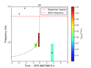
Figures 3 and 3 show two such plots, one centred on the time of an inspiral noise trigger, the other centred on the time of a simulated inspiral signal trigger. In addition to the Omicron triggers, each of these plots show a Newtonian-order time-frequency trajectory for the leading order GW emission of a binary system with mass parameters given by the template where the respective inspiral trigger was seen.

The Omicron triggers of figure 3 are all short-lived ($\sigma_{t}\lesssim 1sec$) and lie scattered around the inspiral track, except for the loudest glitch which appears close to the inspiral trigger time and partially overlaps with the track. However, its central frequency is noticeably away from the inspiral track, an indication that it is likely not an inspiral signal trigger.

When the Omicron algorithm encounters data containing a (simulated) inspiral signal, the inspiral track corresponding to this signal gets covered by a series of Omicron triggers. We see two such triggers in figure 3. Not unexpectedly, the loudest of these triggers sits on the inspiral track with a peak time close to the time of the inspiral signal trigger, i.e. slightly before the time of coalescence (as seen at the detector).

IV.3 Classification features

Using the properties of the inspiral and Omicron triggers, we pass to the random forest algorithm a series of seven inspiral features and fourteen Omicron features, on which the RF will train itself and use to classify noise and signal triggers.

The following lists the inspiral features, briefly explaining each one:

• $\mathrm{SNR_{insp}}$: The inspiral matched filter SNR of a trigger.

• $\mathcal{M}$: The chirp mass of the template used to identify the candidate event, given by Eq. (1)

For the following features, we consider 0.2 second, 2-second, and 20-second time windows $\delta t_{0.1},\delta t_{1},\delta t_{10}$ centred on the time at which the inspiral candidate event occurred, and determine the maximum signal to noise ratio values $\mathrm{SNR_{insp}^{0.1}},\mathrm{SNR_{insp}^{1}},\mathrm{SNR_{insp}^{10}}$ from the SNRs of the triggers within each of the time windows.

• $n_{1,10}$: The number of inspiral triggers within $\delta t_{1,10}$

• $\mathrm{\Delta SNR_{insp}^{0.1,1,10}}$: The difference between the maximum SNR value in each of the time windows $\delta t_{0.1,1,10}$ and the SNR of the trigger on which the window is centred:

  $$\mathrm{\Delta SNR_{insp}^{0.1,1,10}}=\mathrm{SNR_{insp}^{0.1,1,10}}-\mathrm{SNR_{insp}}$$ (14)

The following set of fourteen Omicron features rely entirely on the time at which the inspiral trigger was found. The properties of the loudest Omicron trigger within a time window of $20$ s duration centred on the inspiral trigger time are used as the first five Omicron features:

• $\mathrm{SNR_{omi}^{10}},f^{10}_{s},f^{10}_{e},\tau^{10},\phi^{10}$: The SNR, start frequency, end frequency, center time, center frequency of the loudest Omicron trigger within the $20$ s time window.

Figure 4: The time-frequency box associated to an inspiral search trigger (candidate signal) with coalescence time $t_{c}$ and highest GW frequency $f_{\rm ISCO}$. The inspiral trigger is a maximum of the matched filter time series, where the filter has support between frequencies $f_{\rm low}$ and $f_{\rm ISCO}$.

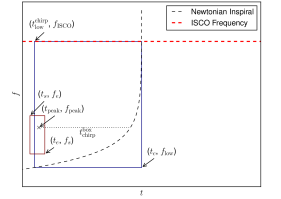
The remaining nine Omicron features are constructed using a time-frequency “box” and an inspiral “track” drawn in the time-frequency plane by assuming $t_{c}$ to be the coalescence time of a binary with chirp mass $\mathcal{M}$ given by the inspiral template: see Figure 4. The lower right corner of the box is the point $(t_{c},f_{\mathrm{low}})$, $t_{c}$ being the time of the inspiral trigger and $f_{\mathrm{low}}=30Hz$, which is close to the lower end of LIGO’s frequency range of detectability. The intersection between the inspiral track and the line of constant frequency $f=f_{\mathrm{low}}$ gives the lower left corner of the box $(t_{\mathrm{low}}^{\mathrm{chirp}},f_{\mathrm{low}})$. The upper right corner of the box is $(t_{c},f_{\mathrm{ISCO}})$, $f_{\mathrm{ISCO}}$ being the GW frequency corresponding to the innermost stable circular orbit, computed using the inspiral template’s chirp mass $\mathcal{M}$ and symmetric mass ratio $\eta$. The upper left corner is the intersection of the line of constant frequency $f=f_{\mathrm{ISCO}}$ and $t=t_{\mathrm{low}}^{\mathrm{chirp}}$.

The set of Omicron triggers that lie within the box are first identified. The properties of these triggers have to satisfy the conditions $\tau>t_{\mathrm{low}}^{\mathrm{chirp}},t_{s}<t_{c},f_{e}>f_{\mathrm{low}},f_{s}<f_{\mathrm{ISCO}}$. This gives us the sixth Omicron feature:

• $n_{\mathrm{box}}$: The number of Omicron triggers found within the time-frequency box.

We then determine the loudest Omicron trigger amongst the $n_{\mathrm{box}}$ triggers within the box, and construct the remaining Omicron features from the properties of this loudest trigger:

• $\mathrm{SNR_{omi}^{box}},t_{s}^{\mathrm{box}},t_{e}^{\mathrm{box}},\sigma_{t}^{{\mathrm{box}}},f_{s}^{\mathrm{box}},f_{e}^{\mathrm{box}},\phi^{\mathrm{box}}$: The SNR, start time, end time, duration, start frequency, end frequency, center frequency of the loudest Omicron trigger in the box.

• $t_{\mathrm{chirp}}^{\mathrm{box}}$: Let $t_{\mathrm{th}}$ be the delay between the coalescence time $t_{c}$ and time-coordinate of the intersection point between the inspiral track and the line $f=\phi^{\mathrm{box}}$. We then define

  $$t_{\mathrm{chirp}}^{\mathrm{box}}=t_{\mathrm{th}}-(t_{c}-\tau^{\mathrm{box}}),$$ (15)

  where $\tau^{\mathrm{box}}$ is the center frequency of the loudest Omicron trigger in the box. $t_{\mathrm{chirp}}^{\mathrm{box}}$ is thus a measure of the temporal separation between the inspiral track and loudest Omicron trigger.

V Random forest tuning and evaluation

In this study we employ the random forest (RF) machine learning algorithm to classify triggers derived from the inspiral matched filter search. We consider each trigger as belonging either to the class of “noise” or “signal”; the trained RF outputs an estimate of the probability of class membership for each trigger supplied to it. The RF has a number of adjustable parameters which may affect the accuracy of this estimate and the computational cost of training and classification. Here we briefly summarize the parameters that were used in our runs; these were arrived at after stages of grid search on a smaller data set. We give both the names used internally in the Python machine learning package scikit-learn Pedregosa et al. (2011) which we use in this study, and a condensed notation used for labelling our plots.

• n_estimators ($N_{t}$): The number of random trees that the RF algorithm is asked to produce. While increasing the number of trees increases the accuracy of the RF’s output, it also enlarges computational costs. Gain in accuracy by adding more trees ultimately starts to saturate, as a consequence of the fact that the training data set is of finite size; after a point, additional trees cannot extract distinct information from the training data relative to their predecessors (see e.g. Baker et al. (2015)). We do not see significant improvements from values above $N_{t}=128$, which is used for all RF implementations here.

• criterion: There are multiple ways by which the quality of a split at a node in a tree may be measured. The “worse” the quality of a split, the larger the mixing of classes of data points at daughter nodes. We use Gini impurity to measure this mixing of classes (scikit-learn also allows the choice of using Shannon entropy).

• min_samples_split: The minimum number of data points required to split an internal node into two daughter nodes. We use the default value $2$.

• min_samples_leaf ($l_{\rm min}$): The minimum number of data points that a daughter node must have. Any split that produces a daughter node with fewer than $l_{\rm min}$ data points is rejected. Reducing $l_{\rm min}$ increases the accuracy of the RF classifier, although a too small value of $l_{\rm min}$ may make the RF prone to over-fitting. Hence this is the main parameter we use to regulate tree size and complexity.

• samples_weight: As discussed in Section II, it is worthwhile to assign weights to signal triggers when training the RF, to model a more astrophysically realistic distribution. To that end, the noise triggers are all set to be equally weighted (unit weights) and the signal triggers are weighted according to the formula

  $$w_{s}=\left(\frac{w}{\rho}\right)^{2},$$ (16)

  where $w$ is a tunable parameter; thus, the smaller the signal SNR, the larger the weight. We also evaluate the RF with the signal triggers all equally weighted; this case will be described as “unit weights”.

Proceeding as described in section II, we generate ROC plots using the RF’s output evaluated on a set of noise and signal triggers, using two-fold cross validation, and compute the $N_{d}$ for a predefined set of $\alpha$s. We repeat the evaluation five times, using the same set of predefined $\alpha$s but a different realization of the two-fold splitting. For each $\alpha$, we then plot the mean $N_{d}$ value and the standard deviation, which we use as a proxy for the statistical error at each point on the ROC.

(a)  LHO data, all triggers weighted equally

(b)  LHO data, signals weighted as $w_{s}=10/\rho^{2}$

(c)  LLO data, all triggers weighted equally

(d)  LLO data, signals weighted as $w_{s}=10/\rho^{2}$

Figure 5: ROC plots for the random forest (RF) classifier for different forest parameters. Each panel shows the expected number of detected signals $N_{d}$ (in arbitrary units) vs. the type I error rate (false positive rate) $\alpha$, estimated by 2-fold cross-validation on trigger sets derived from realistic early Advanced LIGO noise with simulated spinning compact binary inspiral signals. For each plot, the red line shows the ROC of the standard matched filter re-weighted SNR, while the colored lines with error bars show ROCs for the RF classifier with different minimum leaf sizes. Each column corresponds to a different choice of relative weights for signal and noise triggers in training the classifier. All RFs used $N_{t}=128$ trees.

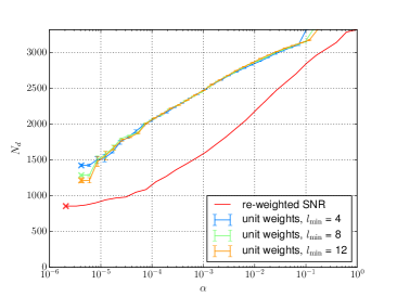
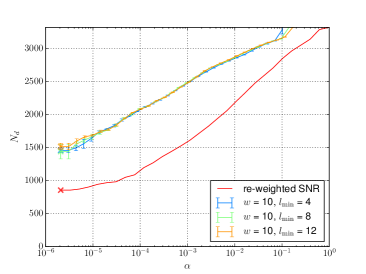
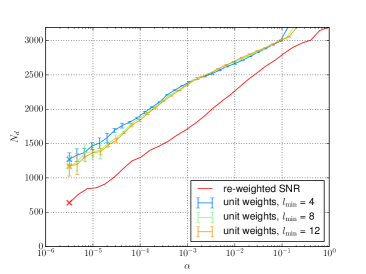
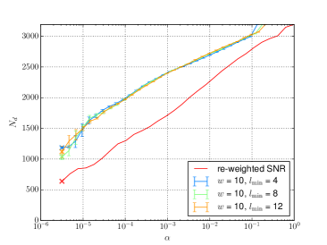
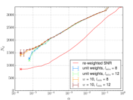
Fig. 5 shows that the RF classification yields a higher expected detection rate than the re-weighted SNR statistic by up to a factor of two at low false positive rates $\alpha\sim 10^{-5}$.The statistical errors in the RF curves estimated from different random cross-validation realizations are small. The efficiency of the RF classification for a given set of data also does not change greatly upon changing the RF parameters, which is an indication of the robustness of the RF algorithm.

Figure 6: Dependence of the RF classification for simulated signal triggers on $\chi^{2}_{r}$ (reduced chi-squared, expectation value $1$ in Gaussian noise) and SNR $\rho$ : color represents the false positive rate $\alpha$ at the threshold of the trigger’s RF score. We show illustrative results from LHO data for the RF classification with unit weights and minimum leaf size 8.

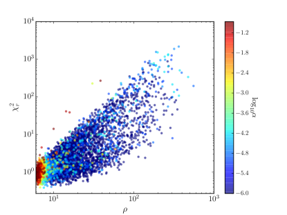
Figure 6 plots $\chi^{2}$ vs SNR for signal triggers and assigns to each trigger a color based on false positive rate $\alpha$, computed using the signal trigger’s probability score (estimated by the RF) as a threshold.

Most signal triggers are located below a diagonal boundary in the $\chi^{2}$-SNR plane. Signal triggers with low SNR are assigned higher $\alpha$ by the RF. The $\alpha$ values decrease by orders of magnitude with increasing SNR, for SNRs between $\sim 6$ and $\sim 10$. Between SNRs $\sim 10$ and $\sim 200$, the plot points maintain a low $\alpha$. Above SNR $\sim 200$, the $\alpha$ starts to increase again. The RF also assigns high $\alpha$ values to all signal triggers above the diagonal boundary and to a few triggers below the boundary.

The higher the false positive rate, the lower the probability score assigned by the RF classifier to the signal trigger. One would expect the RF to output a low probability score if a signal trigger is located in a region with a large number of noise triggers. Indeed, the region above the diagonal boundary, as well as the low- and high-SNR regions are populated by noise triggers.

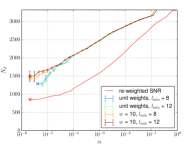
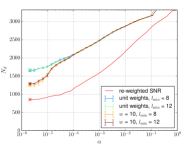
It is clear from Figure 5 that the number of detected signals increases significantly when the RF is used to classify triggers, as compared to the standard re-weighted SNR $\hat{\rho}$ statistic. Naïvely, one might think that using $\hat{\rho}$ as an additional feature for RF classification may further increase the detection efficiency. However, as seen in Figure 7, there is in fact no significant improvement by adding either $\chi^{2}$ or $\hat{\rho}$ as a feature.

(a)  No additional features

(b)  $\chi^{2}$ as an additional feature

(c)  Re-weighted SNR as an additional feature

Figure 7: ROC plots for the RF classifier comparing the standard feature set (left) to the cases where $\chi^{2}$ (centre) or re-weighted SNR $\hat{\rho}$ (right) are added to the feature sets. Axes are as in figure 5. For each plot, the red line shows the ROC of the standard matched filter re-weighted SNR, while the colored lines with error bars show ROCs for the RF classifier with different minimum leaf sizes and weighting schemes. Including $\chi^{2}$ or $\hat{\rho}$ as an additional feature does not significantly increase detection efficiency. We show plots for LHO data only, similar results are obtained for LLO.

V.1 Classification with SNR and chi-squared only

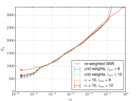
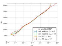
Our results show that a classifier using multiple features derived from triggers close to the time of a candidate event achieves a detection efficiency significantly higher than the standard re-weighted SNR statistic $\hat{\rho}$ via more accurate classification into signal or noise. An interesting question here is whether $\hat{\rho}$, which is built from $\chi^{2}$ and SNR, is an optimal detection statistic given only the values of SNR and $\chi^{2}$? I.e. could a different function of (SNR,$\chi^{2}$) yield a higher efficiency at fixed FPR? To address this question, we employ our RF classifier but use as features only the candidate triggers’ SNR and $\chi^{2}$ values. We find that that the detection efficiency given by the $\hat{\rho}$ statistic and the RF classifier, for a selection of different tree parameters, are nearly equal over almost the entire range of false positive rate $\alpha$. (We also investigated nearest-neighbor and SVM classifiers in various configurations on this 2-d problem and none produced any significant gain over the $\hat{\rho}$ statistic.) While not a proof, this is consistent with $\hat{\rho}$ being close to the optimum detection statistic that can be constructed from $\chi^{2}$ and SNR, at least for our data sets.

Figure 8: ROC plots with LHO (left) and LLO (right) data comparing detection efficiency between the standard re-weighted SNR statistic (red lines) and the RF classifier using only the $\chi^{2}$ and SNR of individual triggers as features, for various choices of forest hyperparameters. The RF classifier reproduces the performance of the standard statistic over a wide range of false positive rate $\alpha$.

VI Discussion

In this study we have shown that a multivariate approach to classifying single-detector events as either (simulated) binary inspiral signals or transient noise artefacts (‘glitches’) can yield a more accurate classification than the currently used time-frequency chi-squared test Allen (2005) in realistic early Advanced LIGO mock data; such an approach can thus be expected to result in a higher detection efficiency for inspiral signals at fixed false alarm probability.

The chi-squared test, which uses only information present in the template matched filter integrand, can effectively downweight many high-amplitude glitches. However, some transient artefacts with moderate SNR values still receive $\chi^{2}$ values typical of signals, although visual inspection of the data suggests a strong inconsistency. These low-$\chi^{2}$ glitches are limiting on the sensitivity of the search to inspiral signals. The use of other test quantities (’features’) computed from data, which can contain information independent of the SNR and $\chi^{2}$ values, enables us to successfully suppress such glitches.

We have conducted a detailed proof of principle study to identify and calculate various features from single-detector data, using both properties of the templated matched filter search (trigger count and maximum SNR over the whole template bank in time windows around a candidate event) and properties of triggers from a sine-Gaussian excess power search using the Q-transform. We then set up a random forest classifier using sets of noise (glitch) triggers obtained from realistic simulated Advanced LIGO noise, and simulated signal triggers obtained from injecting NS-BH inspiral waveforms into the same noise data streams. Note that the (orbitally precessing) injected signals do not lie in the space of (non-spinning) template waveforms; the resulting lack of effectualness is a proxy for unknown systematic uncertainties in NS-BH waveforms which may affect detection.

The performance of the classifier was assessed by calculating the ROC for test data sets under two-fold cross-validation, and we estimated the variance of the ROC by running the cross-validation analysis several times with different random splits. We also explored a range of different hyperparameters in constructing the forest, notably the size of the ‘leaves’ and the relative weighting of signal and noise events.

The figure of merit for the classification is the expected number of signals found at fixed false positive rate (FPR), which is proportional to the volume of space that the search would be sensitive to, assuming that signal events are uniformly distributed through space. We find an increase of a factor 1.5–2 in this sensitive volume at low FPR compared to the “$\chi^{2}$- reweighted SNR” statistic currently used in LIGO searches. The improvement in sensitivity is relatively insensitive to different choices of forest parameters, and is not substantially affected by including or omitting the $\chi^{2}$ or re-weighted SNR values as features. We also checked that, given only the single-detector SNR and $\chi^{2}$ values for individual triggers, the classifier was able to reproduce the ROC of the reweighted SNR statistic; thus, any increase in sensitivity for the full classifier is due to the inclusion of additional information.

This is the first demonstration that a multivariate machine learning classifier acting on single-detector data can outperform the reweighted SNR statistic for inspiral signals. Although a welcome proof of principle, various issues remain to be addressed before such a classifier may be used in production analysis of Advanced LIGO-Virgo data.

The trigger set used here was restricted to relatively high matched filter SNR ($\rho>6.0$) and was clustered over the template bank (selection of the highest-SNR trigger inside given time windows), in order to obtain a manageable number of samples for training the random forest (few$\,\times 10^{5}$); typically under an hour was required for each training round on a single CPU. In current inspiral searches, however, a threshold $\rho>5.5$ is used and no clustering over the bank is applied Abbott et al. (2016b); Usman et al. (2016) thus the total rate of triggers is some orders of magnitude higher. Computational cost might then be addressed by parallelizing the training stage over hundreds of independent trees in the forest, by a decimation process to select a small subset of triggers for training, or possibly use of GPUs.

Since our multivariate classifier is able to efficiently sort signal from noise events in a single detector, we expect that its use within a coincident (two- or more-detector) search would also increase sensitivity to GW inspiral signals. A detection statistic for coincident events (i.e. sets of triggers having consistent parameters over the network) would incorporate the single-detector $\hat{p}$ scores in addition to coincidence parameters: time delays, phase differences and relative amplitudes between detectors Nitz et al. (2017). A more direct application of the method concerns signals which may arrive when only a single detector is observing Callister et al. (2017) as expected in ground-based detector networks with typical duty cycles well below 100$\%$. Although the significance of single-detector candidates is limited by the amount of data available, signals might still be identified if their expected rate, given the detector sensitivity, is high enough and if a reliable method of distinguishing them from noise artefacts is available.

A natural extension of our methodology would be to other types of compact binary coalescence signal templates, specifically for higher-mass systems, given that the traditional $\chi^{2}$ test is less effective for such systems, having shorter duration templates Abbott et al. (2016b); Nitz et al. (2017). An expansion of the method to the early Advanced LIGO stellar-mass binary search space of Abbott et al. (2016b) (template binary mass in $2$-$100$ M_⊙, non-precessing component spins with dimensionless magnitudes up to $0.9895$) is under development for integration in the PyCBC pipeline (for which see https://ligo-cbc.github.io/ and Usman et al. (2016); Dal Canton et al. (2014a)).

Finally, since many transient artefacts in the gravitational wave strain channel could in principle be predicted by use of auxiliary channels that monitor the state of the instrument and the environment Abbott et al. (2016c); Slutsky et al. (2010); Aasi et al. (2015b), we could also consider deriving input features from these channels. This implies a significant increase in the dimensionality and volume of data input to the classifier, requiring machine learning techniques robust to high-dimensional multivariate data where many channels may be redundant or contain their own, irrelevant artefacts (see Biswas et al. (2013) for applications of machine learning to noise artefacts in Initial LIGO data).

References

- Abbott et al. (2016a) B. P. Abbott et al. (Virgo, LIGO Scientific), Phys. Rev. Lett. 116, 061102 (2016a), arXiv:1602.03837 [gr-qc] .
- Abbott et al. (2016b) B. P. Abbott et al. (Virgo, LIGO Scientific), Phys. Rev. D93, 122003 (2016b), arXiv:1602.03839 [gr-qc] .
- Abbott et al. (2016c) B. P. Abbott et al. (Virgo, LIGO Scientific), Class. Quant. Grav. 33, 134001 (2016c), arXiv:1602.03844 [gr-qc] .
- Abbott et al. (2016d) B. P. Abbott et al. (Virgo, LIGO Scientific), Phys. Rev. Lett. 116, 241102 (2016d), arXiv:1602.03840 [gr-qc] .
- Abbott et al. (2016e) B. P. Abbott et al. (Virgo, LIGO Scientific), Phys. Rev. Lett. 116, 241103 (2016e), arXiv:1606.04855 [gr-qc] .
- Abbott et al. (2016f) B. P. Abbott et al. (Virgo, LIGO Scientific), Phys. Rev. X6, 041015 (2016f), arXiv:1606.04856 [gr-qc] .
- Abbott et al. (2017) B. P. Abbott et al. (VIRGO, LIGO Scientific), Phys. Rev. Lett. 118, 221101 (2017), arXiv:1706.01812 [gr-qc] .
- Abbott et al. (2016g) B. P. Abbott et al. (Virgo, LIGO Scientific), Phys. Rev. Lett. 116, 131103 (2016g), arXiv:1602.03838 [gr-qc] .
- Abbott et al. (2016h) B. P. Abbott et al. (Virgo, LIGO Scientific), Astrophys. J. 832, L21 (2016h), arXiv:1607.07456 [astro-ph.HE] .
- Aasi et al. (2015a) J. Aasi et al. (LIGO Scientific), Class. Quant. Grav. 32, 074001 (2015a), arXiv:1411.4547 [gr-qc] .
- Acernese et al. (2015) F. Acernese et al. (VIRGO), Class. Quant. Grav. 32, 024001 (2015), arXiv:1408.3978 [gr-qc] .
- Stevenson et al. (2017) S. Stevenson, C. P. L. Berry, and I. Mandel, (2017), arXiv:1703.06873 [astro-ph.HE] .
- Usman et al. (2016) S. A. Usman et al., Class. Quant. Grav. 33, 215004 (2016), arXiv:1508.02357 [gr-qc] .
- Allen (2005) B. Allen, Phys.Rev. D71, 062001 (2005).
- Allen et al. (2012) B. Allen, W. G. Anderson, P. R. Brady, D. A. Brown, and J. D. E. Creighton, Phys. Rev. D 85, 122006 (2012).
- Abbott et al. (2016i) B. P. Abbott et al. (Virgo, LIGO Scientific), Astrophys. J. 833, 1 (2016i), arXiv:1602.03842 [astro-ph.HE] .
- Abbott et al. (2016j) B. P. Abbott et al. (Virgo, LIGO Scientific), Astrophys. J. Suppl. 227, 14 (2016j), arXiv:1606.03939 [astro-ph.HE] .
- Babak et al. (2013a) S. Babak et al., Phys. Rev. D 87, 024033 (2013a).
- Abbott et al. (2009a) B. Abbott et al. (LIGO Scientific Collaboration), Phys. Rev. D79, 122001 (2009a), arXiv:0901.0302 .
- Abbott et al. (2009b) B. Abbott et al. (LIGO Scientific), Phys.Rev. D80, 047101 (2009b).
- Abadie et al. (2010a) J. Abadie et al. (LIGO Scientific, VIRGO), Phys.Rev. D82, 102001 (2010a).
- Abadie et al. (2012) J. Abadie et al. (LIGO, VIRGO), Phys.Rev. D85, 082002 (2012), arXiv:1111.7314 [gr-qc] .
- Blackburn et al. (2008) L. Blackburn, L. Cadonati, S. Caride, S. Caudill, S. Chatterji, et al., Class.Quant.Grav. 25, 184004 (2008), arXiv:0804.0800 .
- Slutsky et al. (2010) J. Slutsky, L. Blackburn, D. Brown, L. Cadonati, J. Cain, et al., Class.Quant.Grav. 27, 165023 (2010), arXiv:1004.0998 [gr-qc] .
- Aasi et al. (2015b) J. Aasi et al. (LIGO Scientific, VIRGO), Class. Quant. Grav. 32, 115012 (2015b), arXiv:1410.7764 [gr-qc] .
- Rodriguez (2007) A. Rodriguez, Reducing False Alarms in Searches for Gravitational Waves from Coalescing Binary Systems, Master’s thesis, Louisiana State University (2007), arXiv:0802.1376 [gr-qc] .
- Babak et al. (2005) S. Babak, H. Grote, M. Hewitson, H. Lück, and K. A. Strain, Phys. Rev. D 72, 022002 (2005).
- Hanna (2008) C. Hanna, Searching for gravitational waves from binary systems in non-stationary data, Ph.D. thesis, Louisiana State University (2008).
- Harry and Fairhurst (2011) I. W. Harry and S. Fairhurst, Phys.Rev. D83, 084002 (2011), arXiv:1012.4939 [gr-qc] .
- Messick et al. (2017) C. Messick et al., Phys. Rev. D95, 042001 (2017), arXiv:1604.04324 [astro-ph.IM] .
- Robinson et al. (2008) C. Robinson, B. Sathyaprakash, and A. S. Sengupta, Phys.Rev. D78, 062002 (2008).
- Gouaty (2008) R. Gouaty (LIGO Scientific), Class.Quant.Grav. 25, 184006 (2008), arXiv:0805.2412 [gr-qc] .
- Chatterji (1995) S. Chatterji, The search for gravitational wave bursts in data from the second LIGO science run, Ph.D. thesis, Massachusetts Instititute of Technology (1995).
- Collaboration and Collaboration (2011) L. S. Collaboration and V. Collaboration, “Gw100916 blind injection data release,” (2011).
- Robinet (2016) F. Robinet, “Omicron: an algorithm to detect and characterize transient events in gravitational-wave detectors,” (2016), Virgo report VIR-0545B-14.
- Abbott et al. (2009c) B. P. Abbott et al., Phys. Rev. D 80, 102001 (2009c).
- Aasi et al. (2012) J. Aasi et al. (VIRGO), Class.Quant.Grav. 29, 155002 (2012), arXiv:1203.5613 [gr-qc] .
- (38) http://www.stat.berkeley.edu/~breiman/RandomForests/cc_home.htm .
- Baker et al. (2015) P. T. Baker, S. Caudill, K. A. Hodge, D. Talukder, C. Capano, and N. J. Cornish, Phys. Rev. D91, 062004 (2015), arXiv:1412.6479 [gr-qc] .
- Hodge (2014) K. A. Hodge, The search for gravitational waves from the coalescence of black hole binary systems in data from the LIGO and Virgo detectors. Or: A dark walk through a random forest, Ph.D. thesis, Caltech (2014).
- Adams et al. (2013) T. S. Adams, D. Meacher, J. Clark, P. J. Sutton, G. Jones, and A. Minot, Phys. Rev. D88, 062006 (2013), arXiv:1305.5714 [gr-qc] .
- Kim et al. (2015) K. Kim et al., Class. Quant. Grav. 32, 245002 (2015), arXiv:1410.6878 [astro-ph.IM] .
- Abadie et al. (2010b) J. Abadie et al. (VIRGO, LIGO Scientific), Class. Quant. Grav. 27, 173001 (2010b), arXiv:1003.2480 [astro-ph.HE] .
- Searle (2008) A. C. Searle, in Proceedings, 12th Workshop on Gravitational wave data analysis (GWDAW-12) (2008) arXiv:0804.1161 [gr-qc] .
- Sathyaprakash and Dhurandhar (1991) B. S. Sathyaprakash and S. V. Dhurandhar, Phys. Rev. D44, 3819 (1991).
- Finn and Chernoff (1993) L. S. Finn and D. F. Chernoff, Phys. Rev. D 47, 2198 (1993).
- Abbott et al. (2004) B. Abbott et al. (LIGO Scientific), Phys. Rev. D69, 122001 (2004), arXiv:gr-qc/0308069 [gr-qc] .
- Babak et al. (2013b) S. Babak, R. Biswas, P. Brady, D. Brown, K. Cannon, et al., Phys.Rev. D87, 024033 (2013b), arXiv:1208.3491 [gr-qc] .
- (49) “Early aLIGO Configurations: example scenarios toward design sensitivity,” LIGO Document T1200307-v4.
- Dal Canton et al. (2014a) T. Dal Canton et al., Phys. Rev. D90, 082004 (2014a), arXiv:1405.6731 [gr-qc] .
- (51) https://wiki.ligo.org/DASWG/LALSuite .
- Harry et al. (2014) I. W. Harry, A. H. Nitz, D. A. Brown, A. P. Lundgren, E. Ochsner, and D. Keppel, Phys. Rev. D89, 024010 (2014), arXiv:1307.3562 [gr-qc] .
- Ajith et al. (2014) P. Ajith, N. Fotopoulos, S. Privitera, A. Neunzert, and A. Weinstein, Phys. Rev. D89, 084041 (2014), arXiv:1210.6666 [gr-qc] .
- Privitera et al. (2014) S. Privitera, S. R. P. Mohapatra, P. Ajith, K. Cannon, N. Fotopoulos, et al., Phys.Rev. D89, 024003 (2014), arXiv:1310.5633 [gr-qc] .
- Nitz et al. (2013) A. H. Nitz, A. Lundgren, D. A. Brown, E. Ochsner, D. Keppel, and I. W. Harry, Phys. Rev. D88, 124039 (2013), arXiv:1307.1757 [gr-qc] .
- Klimenko et al. (2016) S. Klimenko et al., Phys. Rev. D 93, 042004 (2016), arXiv:1511.05999 [gr-qc] .
- Kanner et al. (2016) J. B. Kanner et al., Phys. Rev. D93, 022002 (2016), arXiv:1509.06423 [astro-ph.IM] .
- Lynch et al. (2017) R. Lynch, S. Vitale, R. Essick, E. Katsavounidis, and F. Robinet, Phys. Rev. D95, 104046 (2017), arXiv:1511.05955 [gr-qc] .
- Dal Canton et al. (2014b) T. Dal Canton, S. Bhagwat, S. Dhurandhar, and A. Lundgren, Class.Quant.Grav. 31, 015016 (2014b), arXiv:1304.0008 [gr-qc] .
- Pedregosa et al. (2011) F. Pedregosa et al., Journal of Machine Learning Research 12, 2825 (2011).
- Nitz et al. (2017) A. H. Nitz, T. Dent, T. Dal Canton, S. Fairhurst, and D. A. Brown, (2017), arXiv:1705.01513 [gr-qc] .
- Callister et al. (2017) T. A. Callister, J. B. Kanner, T. J. Massinger, S. Dhurandhar, and A. J. Weinstein, Class. Quant. Grav. 34, 155007 (2017), arXiv:1704.00818 [astro-ph.IM] .
- Biswas et al. (2013) R. Biswas et al., Phys. Rev. D88, 062003 (2013), arXiv:1303.6984 [astro-ph.IM] .