Fast and accurate computation of projected two-point functions

Abstract

We present the two-point function from fast and accurate spherical Bessel transformation (2-FAST) algorithm for a fast and accurate computation of integrals involving one or two spherical Bessel functions. These types of integrals occur when projecting the galaxy power spectrum $P(k)$ onto the configuration space, $\xi_{\ell}^{\nu}(r)$, or spherical harmonic space, $C_{\ell}(\chi,\chi^{\prime})$. First, we employ the FFTLog transformation of the power spectrum to divide the calculation into $P(k)$-dependent coefficients and $P(k)$-independent integrations of basis functions multiplied by spherical Bessel functions. We find analytical expressions for the latter integrals in terms of special functions, for which recursion provides a fast and accurate evaluation. The algorithm, therefore, circumvents direct integration of highly oscillating spherical Bessel functions.

I Introduction

In standard cosmology, the large-scale structure of the Universe is statistically homogeneous and isotropic and evolved from nearly Gaussian (Maldacena, 2003) primordial curvature perturbations (Mukhanov and Chibisov, 1981; Hawking, 1982; Guth and Pi, 1982; Bardeen et al., 1983) generated during inflation (Starobinskiǐ, 1979; Starobinsky, 1982; Guth, 1981; Sato, 1981; Linde, 1982; Albrecht and Steinhardt, 1982). The statistics of large-scale structure, therefore, are often predicted in terms of the power spectrum $P(k)$ (the two-point correlation function in Fourier space) that reflects the underlying spatial symmetry of the Universe, and that connects directly with the primordial curvature power spectrum. The predicted power spectrum at late times responds sensitively to key cosmological parameters such as the dark energy equation of state, primordial non-Gaussianity parameters, and total mass of neutrinos. This makes the power spectrum a powerful cosmological probe (Percival et al., 2001; Tegmark et al., 2004, 2006; Percival et al., 2007; Blake et al., 2011; Beutler et al., 2014; Rota et al., 2017).

The observed large-scale structure, however, does not enjoy full spatial symmetry because all observations must be done within our past light cone; at each cosmological distance, we observe the large-scale structure at a different time. As a result, the time evolution of large-scale structure genuinely breaks the homogeneity along the radial direction, and we are left only with the spherical symmetry on the two-dimensional sky.

On the sky, the equivalent of the power spectrum $P(k)$ is the angular power spectrum $C_{\ell}$, which is the two-point function in spherical harmonic space. The harmonic-space basis $Y_{\ell m}(\hat{\mathbf{x}})$ is related to the Fourier basis $e^{i\mathbf{k}\cdot\mathbf{x}}$ by Rayleigh’s formula:

$$e^{i\mathbf{k}\cdot\mathbf{x}} =4\pi\sum_{\ell,m}i^{\ell}j_{\ell}(kx)\,Y_{\ell m}(\hat{\mathbf{k}})\,Y^{*}_{\ell m}(\hat{\mathbf{x}}),$$ (1)

so that the angular power spectrum is related to the power spectrum $P(k)$ by integrals of the form

$$w_{\ell\ell^{\prime}}(\chi,\chi^{\prime}) =\frac{2}{\pi}\int_{0}^{\infty}\mathrm{d}{}k\,k^{2}\,P(k)\,j_{\ell}(k\chi)\,j_{\ell^{\prime}}(k\chi^{\prime}),$$ (2)

where $\chi$ and $\chi^{\prime}$ are the comoving angular diameter distances at two different epochs, and $j_{\ell}(z)$ are spherical Bessel functions. Note that we consider the general case of $\ell^{\prime}\neq\ell$, because the contribution from vector or tensor quantities can couple adjacent $\ell$-modes. For example, in order to account for the peculiar velocity effect on redshift-space distortion to linear order, one needs up to $\ell-\ell^{\prime}=\pm 4$. We show an explicit expression of the angular power spectrum $C_{\ell}(\chi,\chi^{\prime})$ of galaxies in redshift space in terms of $w_{\ell\ell^{\prime}}(\chi,\chi^{\prime})$ in App. G. The brute-force numerical integration of Eq. (2) is quite cumbersome and time-consuming because it involves the evaluation of the spherical Bessel functions with high degree $\ell$ and large arguments $k\chi$ at which the $j_{\ell}(k\chi)$ functions are highly oscillatory. It is the oscillatory nature of the spherical Bessel functions that delays the convergence of the numerical integration. Additionally, these integrals are often needed to sample a large area in $\chi$-$\chi^{\prime}$-space.

Although the spherical harmonic basis reflects the underlying spherical symmetry and facilitates data analysis, intuition often works better in configuration space. The prediction for the configuration-space galaxy two-point correlation function that is valid on the spherical sky is often called the wide-angle formula (Szalay et al., 1998; Szapudi, 2004; Papai and Szapudi, 2008) in contrast to the plane-parallel approximation (Kaiser, 1987) that works for small sky coverage. The building blocks of the wide-angle formula are the configuration-space functions $\xi_{\ell}^{\nu}(r)$ defined as

$$\xi^{\nu}_{\ell}(r) \equiv\int_{0}^{\infty}\frac{k^{2}\mathrm{d}{}k}{2\pi^{2}}\,P(k)\,\frac{j_{\ell}(kr)}{(kr)^{\nu}}\,.$$ (3)

Using this notation, the linear two-point correlation function becomes $\xi(r)=\xi_{0}^{0}(r)$, and calculation of the linear redshift-space galaxy correlation function requires $\xi_{2}^{0}(r)$ and $\xi_{4}^{0}(r)$ Hamilton (1992). These functions also appear in calculating the higher-order correlation functions (Slepian and Eisenstein, 2017), the correlation functions of peaks (Bardeen et al., 1986), and nonlinear correlation functions (McCullagh and Szalay, 2014; McEwen et al., 2016; Schmittfull et al., 2016; Fang et al., 2017). Note that, although not as cumbersome and time consuming as Eq. (2), the evaluation of Eq. (3) also involves integrating over spherical Bessel functions that are highly oscillatory in the $k\to\infty$ limit.

In this paper, we shall present a fast and accurate method of calculating the integrations in Eqs. (2)–(3). Specifically, we use the fast Hankel transformation first proposed in Talman (1978) and Siegman (1977), and introduced to the cosmology community in Hamilton (2000). Following Ref. Hamilton (2000), hereafter, we call it an FFTLog transformation. The idea of Talman (1978) is as follows. When changing the integration variables to a logarithmic scale, the spherical Bessel integrations in Eqs. (2)–(3) become convolutions. We then use the convolution theorem to perform the integration: by first Fourier transforming the convolving functions, then multiplying, and inverse Fourier transforming back. The method requires no explicit computation and integration of spherical Bessel functions. Instead, it requires the computation of Gamma functions and the Gauss hypergeometric function ${}_{2}F_{1}$, which are the FFTLog transformation of, respectively, one and two spherical Bessel functions. Therefore, a fast and accurate calculation of Eqs. (2)–(3) boils down to a fast and accurate computation of the Gamma function and Gauss hypergeometric function for any $\ell$ and any ratio $R=\chi^{\prime}/\chi$. We shall achieve this goal by using a recursion.

A recent paper by Assassi et al. (2017) has also proposed a similar algorithm to efficiently calculate the angular two-point function $w_{\ell\ell}(\chi,\chi^{\prime})$. Here, we have further extended the algorithm by studying a fast and accurate method to calculate the Gauss hypergeometric functions, and by including the cases for $\ell\neq\ell^{\prime}$. We also study the choice of parameters such as the biasing parameter $q$ and the size of the FFTLog transformation $N$ in a systematic way.

This paper is organized as follows. In Sec. II we introduce the FFTLog transformation. We present the two-point function from fast and accurate spherical Bessel transformation (2-FAST) algorithm for computing the real-space correlation functions $\xi^{\nu}_{\ell}(r)$ in Sec. III and the harmonic-space two-point correlation functions $w_{\ell\ell^{\prime}}(\chi,\chi^{\prime})$ in Sec. IV. We then apply the 2-FAST algorithm to the galaxy two-point correlation function, to the angular power spectrum of the lensing potential, and to the lensing-convergence-galaxy cross-correlation functions in Sec. V. We conclude in Sec. VI. In App. A we present discrete versions of the equations that we use for the implementation. We study the effect of choosing a different biasing parameter $q$, sampling $N$, and integration interval $G$ in App. B. In App. C we compare our algorithm to a traditional integration method. We lay out the details of our method of calculating the hypergeometric function in App. D, App. E, and App. F. We show explicitly the relation between $w_{\ell\ell^{\prime}}$ and the observed galaxy correlation function $C_{\ell}$ in redshift space in App. G. We summarize a high-accuracy numerical algorithm (the Lucas algorithm Lucas (1995)) that we use to benchmark our result in App. H. Finally, we derive the extended Limber approximation for $\ell\neq\ell^{\prime}$ cases in App. I.

Throughout, we use a flat $\Lambda$CDM universe with $w=-1$, $h=0.6778$, $\Omega_{b}h^{2}=0.022307$, $\Omega_{c}h^{2}=0.11865$, $\Omega_{\nu}h^{2}=0.000638$, $T_{\text{CMB}}=$2.7255\text{\,}\mathrm{K}$$, $n_{s}=0.9672$, and $A_{s}=$2.147\text{\times}{10}^{-9}$$ as the reference cosmology, where $h\equiv H_{0}/$100\text{\,}\mathrm{km}\text{\,}{\mathrm{s}}^{-1}\text{\,}{\mathrm{Mpc}}^{-1}$$.

All numerical implementations in this paper are done in the high-level programming language Julia, which is a just-in-time compiled language developed specifically for scientific numerical computations. We use Julia version 0.6. We run the tests on a laptop with an Intel(R) Core(TM) i7-4750HQ CPU, at $3.1\text{\,}\mathrm{GHz}$ with $11\text{\,}\mathrm{G}\mathrm{i}\mathrm{B}\mathrm{/}\mathrm{s}$ memory access, and a $360\text{\,}\mathrm{M}\mathrm{B}\mathrm{/}\mathrm{s}$ SSD. We have not yet parallelized the code, and all tests were run on a single core. We make the code available publicly at https://github.com/hsgg/twoFAST.

II FFTLog transform of the power spectrum

Figure 1: The linear matter power spectrum, with $q=2$, and $k_{0}=${10}^{-5}\text{\,}\mathrm{\text{$h$}}\text{\,}{\mathrm{Mpc}}^{-1}$$. In gray is the power spectrum, in black the windowed power spectrum [see Eq. (64)], and in dashed blue the Fourier-transformed power spectrum as calculated by the discrete form of Eq. (7). The lower panel shows the relative difference to the input $P(k)$. Here, the number of sampling points between $k_{\mathrm{min}}=${10}^{-5}\text{\,}\mathrm{\text{$h$}}\text{\,}{\mathrm{Mpc}}^{-1}$$ and $k_{\mathrm{max}}=${10}^{3}\text{\,}\mathrm{\text{$h$}}\text{\,}{\mathrm{Mpc}}^{-1}$$ was taken to be $N=1024$.

Figure 2: The absolute value $|\phi^{q}(t)|$ of the FFTLog transform of the biased power spectrum $k^{3-q}P(k)$ for two values of the biasing parameter ${q}$ (colored lines). For comparison, we also show the FFTLog transform of a power spectrum without the baryon acoustic oscillations (BAO) feature for each ${q}$ (gray dashed lines with the same symbols as their BAO counterpart). The gray vertical line shows the maximum $t$ when using $N=512$ sampling points in the interval $k_{\mathrm{min}}=${10}^{-5}\text{\,}\mathrm{\text{$h$}}\text{\,}{\mathrm{Mpc}}^{-1}$$ to $k_{\mathrm{max}}=${10}^{3}\text{\,}\mathrm{\text{$h$}}\text{\,}{\mathrm{Mpc}}^{-1}$$. Here, $m$ is the mode of the Fourier transform, and $G=\ln(k_{\mathrm{max}}/k_{\mathrm{min}})$.

The 2-FAST algorithm is based on the FFTLog transformation Hamilton (2000) of the power spectrum $P(k)$ which can be implemented by a fast Fourier Transform (FFT) of the $P(k)$ sampled at wave numbers $k_{i}$ regularly sampled in logarithmic space. In practice, we perform an FFTLog transformation of the biased power spectrum

$$\left(\frac{k}{k_{0}}\right)^{3-q}P(k) =e^{(3-q)\kappa}P(k_{0}e^{\kappa})\,,$$ (4)

in order to reduce numerical artifacts such as aliasing. Here, $q$ is the biasing parameter and $\kappa$ is the logarithmic variable defined as

$$k =k_{0}e^{\kappa}$$ (5)

with some pivot wave number $k_{0}$. By defining the inverse Fourier transform of the biased power spectrum as $\phi^{q}(x)$, we have the following Fourier pair:

$$\phi^{q}(x) =\int\frac{\mathrm{d}\kappa}{2\pi}\,e^{i\kappa x}\,e^{(3-q)\kappa}\,P(k_{0}e^{\kappa})$$ (6)

$$P(k) =e^{-(3-q)\kappa}\int\mathrm{d}{}x\,e^{-i\kappa x}\,\phi^{q}(x)$$ (7)

We present a discrete version of these equations suitable for numerical implementation in Eq. (63).

Furthermore, in order to reduce ringing, we apply a window function to the biased power spectrum before and after the Fourier transformation. We use the same window function as McEwen et al. (2016) [their Eq. (C.1), and Eq. (64) here]. This choice of the window function ensures that the power spectrum vanishes smoothly at each end of the integration interval, thus reducing ringing.

We calculate the linear matter power spectrum by using CAMB Lewis et al. (2000). However, we have modified CAMB so that the output power spectrum prints more significant digits required for a more accurate FFTLog transformation. Also, when the power spectrum is needed outside of the range of the CAMB output, we extrapolate the linear power spectrum by a power law for both high- and low-$k$ regions

$$\lim_{k\rightarrow 0}P(k) =N_{1}\,k^{n_{1}}$$ (8)

$$\lim_{k\rightarrow\infty}P(k) =N_{2}\,k^{n_{2}-4}\,,$$ (9)

where the limits have been chosen so that both indices are similar to the spectral index, i.e. $n_{1}\simeq n_{2}\simeq n_{s}$. However, we measure $n_{1}$ and $n_{2}$ to ensure that the extrapolated linear power spectrum is smooth. Note that the asymptotic behavior in Eqs. (8)–(9) implies that the FFTLog transform Eq. (6) only converges when

$$n_{2}-1<q<3+n_{1}\,.$$ (10)

For our reference cosmology, $n_{1}\simeq n_{s}=0.967$ and $n_{2}=0.85$, we find $-0.15<q<3.967$.

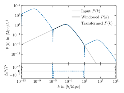
Fig. 1 shows the linear matter power spectrum for our fiducial $\Lambda$CDM cosmology with the biasing parameter $q=2$. The blue dashed line [“Transformed $P(k)$”] shows the result of Eq. (7), the solid gray line [“Input $P(k)$”] shows the input $P(k)$, and the solid black line [“Windowed $P(k)$”] shows the input $P(k)$ amputated by the window function Eq. (64). In this plot, the number of sample points is $N=$1024$$ in the interval $k_{\mathrm{min}}=${10}^{-5}\text{\,}\mathrm{\text{$h$}}\text{\,}{\mathrm{Mpc}}^{-1}$$ to $k_{\mathrm{max}}=${10}^{3}\text{\,}\mathrm{\text{$h$}}\text{\,}{\mathrm{Mpc}}^{-1}$$. The periodicity shown in the figure is due to the use of the FFT. The global slope is due to the use of the biasing parameter $q=2$, since in Eq. (7) the integral is periodic, and it is multiplied by $k^{-1}$.

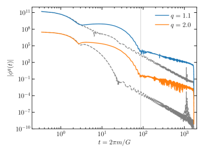
In Fig. 2 we show the FFTLog transformation $\phi^{q}(t)$ of the linear matter power spectrum for two values of the biasing parameter: $q=1.1$ (blue line) and $q=2$ (orange line). In order to highlight the effect from the baryon acoustic oscillations (BAO), we also show $\phi^{q}(t)$ for a linear power spectrum without BAO (gray, dashed lines) that we have calculated from the fitting formula given in Ref. Eisenstein and Hu (1998). The BAO appears in $\phi^{q}(t)$ as the “bump” to the left of the gray vertical line (indicating the Nyquist frequency for the case $N=512$).

In principle, the choice of $q$ within the limits of Eq. (10) should not affect the result of the calculation. When implementing Eqs. (6)–(7) as a finite sum, however, we can reduce the aliasing effect by choosing a proper $q$ value. The rule of thumb is that the Fourier-transformed function will decay quickly (thus, yielding smaller aliasing) when the original function has a broader width (say, measured by the full-width at half maximum). With our parametrization in Eqs. (8)–(9), the slopes of the Fourier-transformed function $e^{(3-q)\kappa}P(k_{0}e^{\kappa})$ are, $e^{3+n_{1}-q}$ and $e^{n_{2}-1-q}$, respectively, at low- and high-$\kappa$ regions. A bigger $q$, therefore, would make the lower-$\kappa$ side shallower and higher-$\kappa$ side steeper. In App. B, we study the aliasing effect for different biasing parameter $q$ and the resolution of FFTLog, $N$. It turns out that the aliasing effect is smaller when the slopes on both sides of the power spectrum are almost equal: $q\simeq 1+(n_{1}+n_{2})/2\simeq 1.9$ (see Fig. 15). This is the choice of the $q$ value that we shall use in Sec. III when we calculate the overlapping of the power spectrum and one spherical Bessel function. It turns out that, however, a smaller $q$-value is desired when calculating $w_{\ell\ell^{\prime}}(\chi,\chi^{\prime})$. We shall justify our choice of the biasing parameter $q$ in App. B.

Note that in the implementation of 2-FAST, we shall use the “coefficients” $\phi^{q}(x)$ of the FFTLog transformation instead of the power spectrum; thus, $\phi^{q}(x)$ is the only $P(k)$-dependent quantity of the integration.

III Projection onto real space: power spectrum overlapping with one spherical Bessel function

We start from the integration of the power spectrum overlapping with one spherical Bessel function:

$$\xi_{\ell}^{\nu}(r)\equiv\int_{0}^{\infty}\frac{k^{2}\mathrm{d}k}{2\pi^{2}}P(k)\frac{j_{\ell}(kr)}{(kr)^{\nu}}\,.$$ (11)

Here, we briefly outline the method and present some examples, including the calculation of the real-space correlation function $\xi(r)\equiv\xi^{0}_{0}(r)$ and its first and second derivatives.

The key observation is that, by introducing logarithmic variables $\kappa$ and $\rho$ such that

$$k =k_{0}e^{\kappa} r =r_{0}e^{\rho}\,,$$ (12)

with some pivot $k_{0}$ and $r_{0}$, the integration in Eq. (11) can be expressed as a convolution:

$$\xi^{\nu}_{\ell}(r) =\frac{k_{0}^{3}e^{-(q_{\nu}+\nu)\rho}}{2\pi^{2}\alpha^{\nu}}\int_{-\infty}^{\infty}\mathrm{d}\kappa\,e^{(3-q_{\nu}-\nu)\kappa}P(k_{0}e^{\kappa})$$

$$\qquad\qquad\qquad\quad\times e^{q_{\nu}(\kappa+\rho)}\,j_{\ell}(\alpha e^{\kappa+\rho})\,.$$ (13)

Here, we define $\alpha=k_{0}r_{0}$, and $q_{\nu}$ is the biasing parameter that may depend on $\nu$. That the convolution in real space is a multiplication in Fourier space motivates us to introduce the Fourier transform of the spherical Bessel function $M_{\ell}^{q_{\nu}}(t)$:

$$e^{q_{\nu}\sigma}\,j_{\ell}(\alpha e^{\sigma}) =\int_{-\infty}^{\infty}\frac{\mathrm{d}{}t}{2\pi}\,e^{i\sigma t}\,M_{\ell}^{q_{\nu}}(t)\,.$$ (14)

Together with $\phi^{q_{\nu}+\nu}(t)$ that we defined earlier in Eq. (6), Eq. (11) becomes

$$\xi^{\nu}_{\ell}(r) =\frac{k_{0}^{3}e^{-(q_{\nu}+\nu)\rho}}{\pi\alpha^{\nu}}\int_{-\infty}^{\infty}\frac{\mathrm{d}{}t}{2\pi}\,e^{i\rho t}\,\phi^{q_{\nu}+\nu}(t)\,M_{\ell}^{q_{\nu}}(t)\,.$$ (15)

Eq. (15) is the key equation for the 2-FAST algorithm. The cosmology-dependent part $\phi^{q_{\nu}+\nu}(t)$ is calculated as the FFTLog transformation of the power spectrum as described in Sec. II. The cosmology-independent part $M^{q_{\nu}}_{\ell}(t)$ is calculated analytically by inverting its definition Eq. (14). Defining a variable $s=\alpha e^{\sigma}$, the inverse Fourier transformation may be written as

$$M_{\ell}^{q_{\nu}}(t) =\int_{-\infty}^{\infty}\mathrm{d}{}\sigma\,e^{-it\sigma}\,e^{q_{\nu}\sigma}\,j_{\ell}(\alpha e^{\sigma})$$

$$=\alpha^{it-q_{\nu}}\int_{0}^{\infty}\mathrm{d}{}s\,s^{q_{\nu}-1-it}\,j_{\ell}(s)$$

$$\equiv\alpha^{it-q_{\nu}}\,u_{\ell}(q_{\nu}-1-it)\,.$$ (16)

The integral $u_{\ell}(n)$ is given by

$$u_{\ell}(n) \equiv\int_{0}^{\infty}\mathrm{d}{}s\,s^{n}\,j_{\ell}(s)=2^{n-1}\sqrt{\pi}\,\frac{\Gamma\big{[}\frac{1}{2}(1+\ell+n)\big{]}}{\Gamma\big{[}\frac{1}{2}(2+\ell-n)\big{]}}$$ (17)

when $\Re(n-1)<0$ and $\Re(n+\ell)>-1$. Hereafter, $\Re(z)$ denotes the real part of a complex number $z$. For our case,

$$n =q_{\nu}-1-it\,.$$ (18)

For $r_{0}$ we recommend the choice $r_{0}\sim 1/k_{\mathrm{max}}$.

III.1 The biasing parameter $q$

How do we need to choose the biasing parameter $q$? First, the integration $M_{\ell}^{q_{\nu}}(t)$ restricts the biasing parameter $q_{\nu}$ to the range

$$-\ell<q_{\nu}<2\,.$$ (19)

In addition, the FFTLog transformation exists when $n_{2}-1<q_{\nu}+\nu<3+n_{1}$ [Eq. (10)]. Combining the two conditions, we find

$$\mathrm{max}(n_{2}-1-\nu,-\ell)<q_{\nu}<\mathrm{min}(3+n_{1}-\nu,2)\,,$$ (20)

or $\mathrm{max}(-0.15-\nu,-\ell)<q_{\nu}<\mathrm{min}(3.967-\nu,2)$ for our reference cosmology. Note that Eq. (20) implies that a valid value of $q_{\nu}$ exists only if

$$n_{2}-3<\nu<3+n_{1}+\ell\,,$$ (21)

or $-2.15<\nu<\ell+3.967$ for our reference cosmology, and this is the condition of convergence for the integral Eq. (11) when using the asymptotic behavior of the power spectrum in Eqs. (8)–(9).

As we show in App. B, there is an aliasing effect from the discrete implementation of the integration in Eq. (6). We shall first choose a finer Fourier resolution $N$ in order to ensure that all the relevant Fourier modes are summed over in Eq. (15). Then, our first choice for $q_{\nu}$ is $q_{\nu}=1.9-\nu$, because the aliasing effect in $\phi^{q}(t)$ is small for $q=q_{\nu}+\nu=1.9$. If $1.9-\nu$ falls outside the range in Eq. (20), then we choose

$$q_{\nu} =\frac{1}{3}(q_{\nu,\mathrm{min}}+2q_{\nu,\mathrm{max}})\,,$$ (22)

where $q_{\nu,\mathrm{min}}$ and $q_{\nu,\mathrm{max}}$ are the boundaries given in Eq. (20). Note that we weight slightly toward the higher-$q_{\nu}$ values. We show that this choice of $q_{\nu}$ gives accurate results for a wide range of $(\ell,\nu)$ combinations in App. B.

III.2 Results: Accuracy

Figure 3: Accuracy comparison for different implementations of $\xi_{\ell}^{\nu}(r)$. Left: The upper panel shows the real-space correlation function $\xi^{0}_{0}(r)$ and its first and second derivatives calculated with the 2-FAST algorithm (dashed colored lines) and with the quadosc algorithm (solid gray lines). To calculate the first and second derivatives with the 2-FAST algorithm we use Eqs. (23)–(24). For the quadosc algorithm we take the derivatives by creating a fifth-order spline of $\xi^{0}_{0}(r)$, and taking derivatives of the spline. The lower panel shows the relative difference between the 2-FAST results and the quadosc results. The difference is generally less than $\sim 0.05\text{\,}\mathrm{\char 37\relax}$, except at zero crossings, and at very small and large separations $r$. The differences at $r\gtrsim$150\text{\,}{\mathrm{\text{$h$}}}^{-1}\text{\,}\mathrm{Mpc}$$ are likely due to pathologies in the quadosc algorithm, as closer inspection reveals unnatural oscillations in the quadosc curve, see Fig. 4. Right: The same as on the left, except for $\xi^{0}_{2}(r)$, $\xi^{0}_{4}(r)$, and $\xi^{3}_{1}(r)$. For the 2-FAST algorithm we used $N=1024$, $k_{\mathrm{min}}=${10}^{-5}\text{\,}\mathrm{\text{$h$}}\text{\,}{\mathrm{Mpc}}^{-1}$$, and $k_{\mathrm{max}}=${10}^{3}\text{\,}\mathrm{\text{$h$}}\text{\,}{\mathrm{Mpc}}^{-1}$$. Increasing $N$ leads to better agreement between 2-FAST and quadosc.

Figure 4: A zoom-in of Fig. 3 at large $r$. Here we chose $N=16384$ for the 2-FAST algorithm (green dashed curve) to get a more dense sampling in $r$. The quadosc curve (solid gray) shows unnatural erratic behavior. Since the second derivative $\xi^{\prime\prime}(r)$ is expected to be smooth, it is likely that this erratic behavior is due to limitations of the quadosc algorithm.

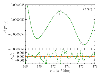
We assess the accuracy of the 2-FAST algorithm by comparing the result with a slow, but accurate benchmark algorithm. The quadosc (Press et al., 2007) algorithm can integrate oscillatory functions accurately over an infinite interval. The quadosc algorithm works by integrating between successive zeros of the integrand using Gauss-Kronrod quadrature, and then using a series convergence acceleration to sum up the terms effectively out to infinity. For the convergence acceleration we use the Levin $u$-transform as described in Press et al. (2007). In addition, we also verified that our results agree with the results from FFTLog (Hamilton, 2000) to within the accuracy achievable with quadosc.

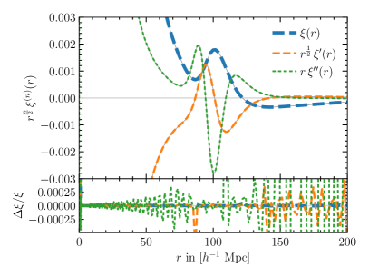
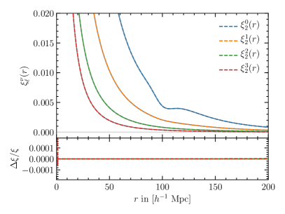
Fig. 3 compares the result from 2-FAST with the result from quadosc. The left panel shows the configuration-space two-point correlation function [$\xi(r)=\xi^{0}_{0}(r)$, thick blue dashed line] and its first [$r^{1/2}\xi^{\prime}(r)$, orange dashed lines] and second [$r\xi^{\prime\prime}(r)$, green dashed line] derivatives. Using the identities for the spherical Bessel function, $(2\ell+1)\,j^{\prime}_{\ell}(x)=\ell\,j_{\ell-1}(x)-(\ell+1)\,j_{\ell+1}(x)$ and $(2\ell+1)j_{\ell}(x)/x=j_{\ell-1}(x)+j_{\ell+1}(x)$, the first and second derivatives of $\xi(r)$ can also be calculated using the 2-FAST algorithm:

$$\xi^{\prime}(r) =-\frac{1}{r}\xi^{-1}_{1}(r)$$ (23)

$$\xi^{\prime\prime}(r) =\frac{1}{r^{2}}\big{[}\xi^{-2}_{2}(r)-\xi^{-1}_{1}(r)\big{]}$$ (24)

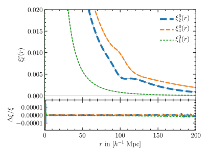
The right panel of Fig. 3 shows the results for $\xi^{0}_{2}(r)$ (blue dashed line), $\xi^{0}_{4}(r)$ (orange dashed line), and $\xi^{3}_{1}(r)$ (green dashed lines). For all cases, we show the corresponding results of the quadosc algorithm as solid gray lines. For the 2-FAST calculation, we used $N=1024$, $k_{\mathrm{min}}=${10}^{-5}\text{\,}\mathrm{\text{$h$}}\text{\,}{\mathrm{Mpc}}^{-1}$$, $k_{\mathrm{max}}=${10}^{3}\text{\,}\mathrm{\text{$h$}}\text{\,}{\mathrm{Mpc}}^{-1}$$, and $r_{0}=${10}^{-3}\text{\,}{\mathrm{\text{$h$}}}^{-1}\text{\,}\mathrm{Mpc}$$.

To facilitate the comparison better, in the lower panels of Fig. 3, we show the fractional difference between the derivatives calculated from the two methods (quadosc and its numerical derivatives and 2-FAST). For $\xi_{0}^{0}$, $\xi_{2}^{0}$ and $\xi_{4}^{0}$, the difference between the two methods is smaller than $\sim 0.05\text{\,}\mathrm{\char 37\relax}$, and the accuracy improves when increasing the sampling size $N$. The derivatives are less accurate, in particular, at very small $r$, at zero crossings, and at $r\gtrsim$150\text{\,}{\mathrm{\text{$h$}}}^{-1}\text{\,}\mathrm{Mpc}$$. The accuracy of the $\xi_{2}^{-2}(r)$ term is worst, since more negative $\nu$ puts more weight on small scale structure.

The residuals are particularly large for the second derivative. We find that the oscillatory features in the residuals of the second derivative on small scales $r<$100\text{\,}{\mathrm{\text{$h$}}}^{-1}\text{\,}\mathrm{Mpc}$$ are improved when increasing the sampling frequency $N$. However, on large scales ($r>$100\text{\,}{\mathrm{\text{$h$}}}^{-1}\text{\,}\mathrm{Mpc}$$) we find that the discrepancies reflect limitations of the quadosc algorithm. In Fig. 4 we show a zoom-in of Fig. 3 for the second derivative $\xi^{\prime\prime}(r)$, where for the 2-FAST algorithm we used $N=16384$ in order to get a dense sampling in $r$ space. The gray curve, again, shows the result from using the quadosc algorithm to calculate $\xi(r)$, taking a fifth-order spline, and then using the second derivative of the spline function. The quadosc curve shows unnatural erratic behavior. Since the second derivative should be a smooth function, it is likely that the differences between the 2-FAST and the quadosc results are due to limitations of our implementation of the quadosc algorithm and are not a limitation of the 2-FAST method.

III.3 Results: Performance

Figure 5: Performance of the 2-FAST algorithm as a function of sampling points $N$. We show the timings of three runs at each $N$, Run 1 to 3, each run having equal settings. The algorithm achieves $\sim 1.3\text{\,}\mathrm{ms}$ performance for $N=1024$.

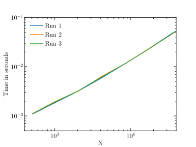
In Fig. 5 we show the performance of the 2-FAST algorithm as a function of the number of sampling points $N$. The figure shows that with the 2-FAST algorithm we can calculate each curve in Fig. 3 in $\sim 1.3\text{\,}\mathrm{ms}$ on the test laptop that we describe at the end of Sec. I. The majority of the time is spent in the FFT, for which we use the Fastest Fourier Transform in the West (FFTW) package. Note that the memory allocation time of Julia adds to the run time, so further optimization using a lower-level language is still possible, if necessary. The FFTLog software (Hamilton, 2000) has similar performance, though a different feature set.

IV Projection onto spherical harmonic space

We now turn to the case with two spherical Bessel functions, Eq. (2). With the biasing parameter $q$, Eq. (2) becomes

$$w_{\ell\ell^{\prime}}(\chi,\chi^{\prime}) =\frac{2}{\pi}\int_{0}^{\infty}\mathrm{d}{}k\,k^{2-q}\,P(k)\,k^{q}j_{\ell}(k\chi)\,j_{\ell^{\prime}}(k\chi^{\prime})\,.$$ (25)

As in Sec. III, we shall turn Eq. (25) into a convolution integral by introducing logarithmic variables $\kappa$, $\rho$, and the ratio $R=\chi^{\prime}/\chi$ which are defined as

$$\frac{k}{k_{0}} =e^{\kappa} \frac{\chi}{\chi_{0}} =e^{\rho} \chi^{\prime} =R\chi=R\chi_{0}e^{\rho}\,,$$ (26)

for some pivot wave number $k_{0}$ and pivot distance $\chi_{0}$. Then, Eq. (25) becomes

$$w_{\ell\ell^{\prime}}(\chi,R) =\frac{2k_{0}^{3}}{\pi}\,e^{-q\rho}\int_{-\infty}^{\infty}\mathrm{d}{}\kappa\,e^{(3-q)\kappa}\,P(k_{0}e^{\kappa})$$

$$\qquad\quad\times e^{q(\kappa+\rho)}j_{\ell}(\alpha e^{\kappa+\rho})\,j_{\ell^{\prime}}(R\alpha e^{\kappa+\rho})\,.$$ (27)

where $\alpha=k_{0}\chi_{0}$. Parallel to Sec. III, we introduce the Fourier transformation of the multiplication of two spherical Bessel functions $M_{\ell\ell^{\prime}}^{q}(t,R)$ as

$$e^{q\sigma}\,j_{\ell}(\alpha e^{\sigma})\,j_{\ell^{\prime}}(\beta e^{\sigma}) =\int\frac{\mathrm{d}{}t}{2\pi}\,e^{it\sigma}\,M_{\ell\ell^{\prime}}^{q}(t,R)\,.$$ (28)

We can now rewrite Eq. (27) by using $\phi^{q}$ and $M_{\ell\ell^{\prime}}^{q}$ as

$$w_{\ell\ell^{\prime}}(\chi,R) =4k_{0}^{3}\,e^{-q\rho}\int\frac{\mathrm{d}{}t}{2\pi}\,e^{it\rho}\,\phi^{q}(t)\,M_{\ell\ell^{\prime}}^{q}(t,R)\,,$$ (29)

where $\chi$ is related to $\rho$ by Eq. (26). Eq. (29) is the core of the 2-FAST algorithm for calculating the angular power spectrum in harmonic space. We show the discrete version of Eq. (29) that we use for the implementation in App. A.3. We have already discussed the FFTLog transformation in Sec. II, and the key to evaluate $w_{\ell\ell^{\prime}}(\chi,R)$ is computing $M_{\ell\ell^{\prime}}^{q}(t,R)$, which we shall turn to next.

IV.1 Fourier transform of two spherical Bessel functions

Figure 6: In order to calculate the Fourier transform of two spherical Bessel functions $M^{q}_{\ell\ell^{\prime}}(t,R)$, we employ recursions along the paths in $\ell\ell^{\prime}$ space shown in this figure for $\ell_{\mathrm{max}}=8$. Each node shows its $(\ell,\ell^{\prime})$ coordinates. For $R\leq 1$ we start at $\ell_{\mathrm{max}}$ with $\Delta\ell=\ell^{\prime}-\ell=4$, and proceed down along the path $\ell^{\prime}=\ell+4$ until $\ell=0$. At each $\ell$, we then proceed with a recursion $\Delta\ell\rightarrow\Delta\ell-2$ until $\Delta\ell=-4$. The gray underlying squares centered on the white nodes indicate the values of $w_{\ell\pm 2,\ell\pm 2}$ which are needed to calculate the $C_{\ell}$ with linear redshift-space distortion (see App. G). In gray we also indicate the start of the recursion for $R>1$, which is stable along the paths $\ell^{\prime}=\ell-4$ and $\Delta\ell\rightarrow\Delta\ell+2$ (not shown). The recurrence relations and their stability properties are derived in App. E and App. F.

compat=1.13

Figure 7: Overview of the 2-FAST algorithm of calculating $w_{\ell\ell^{\prime}}(\chi,\chi^{\prime})$. Starting at the top left, we start by calculating the cosmology-independent part $M^{q}_{\ell\ell}(t,R)=A_{\ell,\Delta\ell}\,\,{}_{2}F_{1,\ell,\Delta\ell}$ at $\ell=0$ and $\Delta\ell=\pm 4$. The plus sign is chosen for $R\leq 1$, and the negative sign for $R>1$. Following App. E the cosmology-independent part is calculated for $\ell_{\mathrm{max}}$ from $\ell=0$. Then, the recursion from $\ell_{\mathrm{max}}\rightarrow 0$ is used, and at each step the products $w_{\ell,\ell\pm(0,2,4)}(\chi,R)$ are calculated. Note that everything to the left of where the Fourier transform $\phi^{q}(t)$ of the power spectrum enters is independent of the cosmology and can be precomputed. Thick arrows signify paths that need to be taken multiple times as the recursion over $\ell$ progresses. Furthermore, since the transformation from $w_{\ell\ell^{\prime}}(\chi,\chi^{\prime})$ to $w_{\ell,jj^{\prime}}(\chi,\chi^{\prime})$ is linear (see App. G), that can also be done before multiplying by $\phi^{q}(t)$. However, this does not significantly change the method here.

The $P(k)$-independent part $M_{\ell\ell^{\prime}}^{q}(t,R)$ is given by the Fourier transformation of the product of two spherical Bessel functions:

$$M^{q}_{\ell\ell^{\prime}}(t,R) =\int\mathrm{d}{}\sigma\,e^{(q-it)\sigma}\,j_{\ell}(\alpha e^{\sigma})\,j_{\ell^{\prime}}(R\alpha e^{\sigma})$$

$$=\alpha^{-1}\int\mathrm{d}{}s\,\left(\frac{s}{\alpha}\right)^{q-1-it}\,j_{\ell}(s)\,j_{\ell^{\prime}}(Rs)$$

$$=\alpha^{it-q}\int\mathrm{d}{}s\,s^{q-1-it}\,j_{\ell}(s)\,j_{\ell^{\prime}}(Rs)$$

$$=\alpha^{it-q}\,U_{\ell\ell^{\prime}}(R,q-1-it)\,,$$ (30)

where $s=\alpha e^{\sigma}$, or $\sigma=\ln(s/\alpha)$, and $U_{\ell\ell^{\prime}}(R,n)$ is given in terms of the Gauss hypergeometric function ${}_{2}F_{1}$ as

$$U_{\ell\ell^{\prime}}(R,n)$$

$$=2^{n-2}R^{\ell^{\prime}}\pi\,\frac{\Gamma\big{[}(1+\ell+\ell^{\prime}+n)/2\big{]}}{\Gamma\big{[}(2+\ell-\ell^{\prime}-n)/2\big{]}\Gamma\big{[}\frac{3}{2}+\ell^{\prime}\big{]}}$$

$$\quad\times{}_{2}F_{1}\bigg{(}\frac{-\ell+\ell^{\prime}+n}{2},\frac{1+\ell+\ell^{\prime}+n}{2};\frac{3}{2}+\ell^{\prime};R^{2}\biggl{)}\,,$$ (31)

which we obtained from Mathematica (Wolfram Research, Inc., ). Here, $n=q-1-it$. Note that the general expression Eq. (31) is valid for $|R|<1$, $\Re(n)<2$ and $\Re(\ell+\ell^{\prime}+n)>-1$. Furthermore, for $R=1$, the Gauss hypergeometric function converges only if $\Re(1-n)>0$. These conditions put constraints on the choice of the biasing parameter $q$:

$$-\ell-\ell^{\prime}<q<2\,.$$ (32)

The method for calculating the function $U_{\ell\ell^{\prime}}(R,n)$, however, may put further constraints on $q$. For example, when evaluating $U_{\ell\ell^{\prime}}(R,n)$ by recursion (see below for the details of the recursion), we need to know $U_{\ell\ell^{\prime}}$ at $\ell=\ell^{\prime}=0$. In that case, the Gamma function in the numerator of Eq. (31) becomes infinite when $n$ is a negative odd integer, which happens for $t=0$ and nonpositive even integer values of $q$. Hence, we have the further constraint

$$q \neq-2m\qquad\text{for }m=0,1,\cdots\,.$$ (33)

Furthermore, $q\neq 1$ is required for our implementation of the case $R=1$; see App. E.3.1. For the calculation of $w_{\ell\ell^{\prime}}(\chi,\chi^{\prime})$, we find that $q<1.5$ is required to suppress the aliasing effect associated with the convolution for $\chi,\chi^{\prime}\gtrsim$10\text{\,}{\mathrm{\text{$h$}}}^{-1}\text{\,}\mathrm{Mpc}$$ (see App. B).

The $R=\chi^{\prime}/\chi>1$ cases can also be obtained from Eq. (31) which is valid only for $|R|<1$, because by simply changing the integration variable from $s$ to $s^{\prime}=Rs$, Eq. (30) becomes

$$M_{\ell\ell^{\prime}}^{q}(t,R) =(R\alpha)^{it-q}\int\mathrm{d}{}s^{\prime}\,s^{\prime q-1-it}\,j_{\ell}(R^{-1}s^{\prime})\,j_{\ell^{\prime}}(s^{\prime})$$

$$=(R\alpha)^{it-q}\,U_{\ell^{\prime}\ell}(R^{-1},q-1-it)\,.$$ (34)

Note that $M_{\ell\ell^{\prime}}$ is now proportional to $U_{\ell^{\prime}\ell}$. We use Eq. (34) when calculating for $R>1$ cases.

Now, the efficiency and accuracy of the $2$-FAST algorithm depends on our ability to calculate the Gauss hypergeometric function ${}_{2}F_{1}$ in Eq. (31). Here, we use a set of recurrence relations based on contiguous relations for the Gauss hypergeometric function that we list in Eqs. (88a)–(88h). We describe the details of the recursion in App. E and App. F, and outline the key procedure here. In particular, our implementation is based upon the following three properties of ${}_{2}F_{1}$ in Eq. (31): (A) the backward recursion $\ell\to\ell-1$ is stable in all cases of interest; (B) the recursion $\Delta\ell=4\to\Delta\ell=-4$ is stable for $R<1$ cases; (C) the recursion $\Delta\ell=-4\to\Delta\ell=4$ is stable for $R>1$ cases, for $\Delta\ell\equiv\ell-\ell^{\prime}$. Note that from Eq. (34), (B) implies (C). Here, we call a recursion stable when the error decays as the recursion proceeds.

Miller’s algorithm Bickley et al. (1952) exploits the property (A) and runs the recursion backwards for a fixed $\Delta\ell$. Here, we extend Miller’s algorithm by using all three properties as follows. First, we calculate the backward recursion from high $\ell_{\mathrm{seed}}$ down to $\ell=0$ for the fixed $\Delta\ell=4$ (when $R<1$) and $\Delta\ell=-4$ (when $R>1$) cases. We then run recursions through the $\Delta\ell$ direction to complete the calculation. The recursion paths in $\ell\ell^{\prime}$ space are shown in Fig. 6.

In order to run the recursion backward, we need to set up the initial condition at some large multipole moment $\ell_{\mathrm{seed}}$. We then run the backward recursion down to $\ell=0$ where we can fix the normalization by using the analytical expression of ${}_{2}F_{1}$ at $\ell=0$. Because the backward recursion is stable, the only requirement is that we must choose $\ell_{\mathrm{seed}}$ sufficiently larger than $\ell_{\mathrm{max}}$ (maximum $\ell$ desired) so that any inaccuracy in the initial condition decays sufficiently at $\ell_{\mathrm{max}}$. We ensure that by requiring that the ${}_{2}F_{1}$ at $\ell_{\mathrm{max}}$ for different starting $\ell_{\mathrm{seed}}$ values converge within a fractional error of $10^{-10}$ [see Eq. (102)]. As the error decays throughout the backward recursion, initial conditions do not have to be exact. The closer the initial conditions are to the true ${}_{2}F_{1}$, however, the more efficient the algorithm is, since a smaller $\ell_{\mathrm{seed}}$ would be sufficient. For the $R\ll 1$ case, we use the asymptotic behavior of the recurrence relation in the limit $\ell\to\infty$ to set the initial conditions. For the $R\sim 1$ case, it turns out that, albeit noisy, the forward recursion provides a reasonable initial condition at $\ell_{\mathrm{seed}}$. We, therefore, set up the initial condition by running the forward recursion to $\ell_{\mathrm{seed}}$, and then we apply the backward recursion.

For the $R=1$ case, we use an analytical expression for the hypergeometric function ${}_{2}F_{1}$,

$${}_{2}F_{1}\bigg{(}\frac{-\ell+\ell^{\prime}+n}{2},\frac{1+\ell+\ell^{\prime}+n}{2};\frac{3}{2}+\ell^{\prime};1\biggl{)}$$

$$=\frac{\Gamma\big{(}\frac{3}{2}+\ell^{\prime}\big{)}\,\Gamma\big{(}1-n\big{)}}{\Gamma\big{[}\frac{1}{2}\big{(}3+\ell^{\prime}+\ell-n\big{)}\big{]}\,\Gamma\big{[}\frac{1}{2}\big{(}2+\ell^{\prime}-\ell-n\big{)}\big{]}}\,,$$ (35)

which we use to initialize the recursion at $\ell_{\mathrm{max}}$.

IV.2 From $M_{\ell\ell^{\prime}}^{q}(t,R)$ to angular power spectra

Figure 8: The transformation matrix $T_{\ell n}$ given in Eq. (IV.2) multiplied by $k_{n}^{-1}$ for a Dirac-delta window function centered around $\chi_{n^{\prime}}=$2370\text{\,}{\mathrm{\text{$h$}}}^{-1}\text{\,}\mathrm{Mpc}$$ for $R=0.75$ (left) and $R=1$ (right). The color bar shows the value of $k_{n}^{-1}T_{\ell n}$ on a nonlinear $\sinh^{-1}$ scale. The minor tick marks in the color bars are linearly spaced. At high $k$, the transformation matrix is smooth, since for each $k_{n}$, $T_{\ell n}$ represents an integral over multiple oscillations of the spherical Bessel functions. At high $\ell$, the transformation matrix is significant only along $k_{n}\sim\sqrt{\ell(\ell+1)}/\chi_{n^{\prime}}$ (gray dotted line), which shows that Limber’s approximation should work well in this regime.

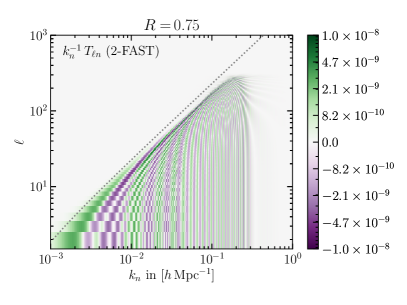
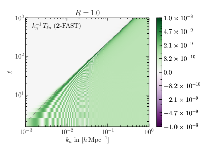
Eqs. (29)–(31) describe our method of computing an integral over two spherical Bessel functions. A discrete version is given in App. A.3. We give an overview of the method in Fig. 7.

In linear theory, all harmonic-space power spectra are linear in $P(k)$, and they can be calculated as a linear combination of $w_{\ell\ell^{\prime}}(\chi,\chi^{\prime})$. One such example is the linear, redshift-space, galaxy power spectrum $C_{\ell}$ that we present in App. G. For these cases, we can carry out the $P(k)$-independent part of the calculation with $M_{\ell\ell^{\prime}}^{q}$ before the power spectrum enters the calculation. That is, for a given set of spherical observables that are linearly related to $P(k)$, the 2-FAST method naturally breaks down the calculation into the $P(k)$-dependent $\phi^{q}$ and the $P(k)$-independent part which can be precalculated.

As an example, consider cross-correlating two linear galaxy density fields spread over redshift ranges centered around, respectively, $z_{1}$ and $z_{2}$ with the survey radial window functions, respectively, $\mathcal{W}_{1}(\chi)$ and $\mathcal{W}_{2}(\chi)$. The angular power spectrum in this case is given by

$$C_{\ell}=b_{1}^{2}\int\mathrm{d}\chi_{1}\int\mathrm{d}\chi_{2}\;\mathcal{W}_{1}(\chi_{1})\mathcal{W}_{2}(\chi_{2})w_{\ell\ell}(\chi_{1},\chi_{2}),$$ (36)

which can be calculated by using Eq. (29)

$$C_{\ell} =4k_{0}^{3}b_{1}^{2}\int\mathrm{d}\chi_{1}\int\mathrm{d}\chi_{2}\;\mathcal{W}_{1}(\chi_{1})\mathcal{W}_{2}(\chi_{2})$$

$$\times e^{-q\rho}\int\frac{dt}{2\pi}\,e^{it\rho}\phi^{q}(t)M^{q}_{\ell\ell^{\prime}}(t,R)$$

$$=8k_{0}^{3}\chi_{0}^{2}b_{1}^{2}\int\frac{dt}{2\pi}\,\phi^{q}(t)$$

$$\times\int\mathrm{d}\rho\int_{0}^{1}\mathrm{d}R\,e^{(2-q+it)\rho}\,\mathcal{W}_{1}(e^{\rho})\,\mathcal{W}_{2}(Re^{\rho})\,M^{q}_{\ell\ell^{\prime}}(t,R)\,.$$ (37)

The second line of the integration is independent from the power spectrum, and could be calculated for given radial window functions. Since the radial window functions $\mathcal{W}_{i}(\chi)$ are cosmology dependent, encompassing the linear growth factor, redshift-distance relation and so on, we do not further investigate this approach in this paper. Upon the quantification of these radial dependences, rearranging the integrals as in Eq. (37) should result in a fast and accurate calculation.

Alternatively, we can also define the transformation matrix between the Fourier-space power spectrum $P(k)$ and angular power spectrum $w_{\ell\ell^{\prime}}$. We write Eq. (29) with Eq. (6) as

$$w_{\ell\ell^{\prime}}(\chi,R) =\int\frac{\mathrm{d}k}{k}\,P(k)\,\bigg{[}\frac{2}{\pi}\,k^{3}e^{-q(\kappa+\rho)}\,$$

$$\quad\times\int\frac{dt}{2\pi}\,e^{it(\kappa+\rho)}\,M^{q}_{\ell\ell^{\prime}}(t,R)\bigg{]}\,,$$ (38)

If we evaluate the integrals as written using the definition of $M^{q}_{\ell\ell^{\prime}}(t,R)$ in Eq. (28), we recover Eq. (2). However, for implementation on a computer, the integrals are approximated as sums over discrete $k_{n}$ and $t_{m}$. Using the discrete versions of our algorithm in App. A, the term in brackets and the measure become

$$T^{\ell^{\prime},q}_{\ell n}(\chi_{n^{\prime}},R) =\frac{2}{\pi}\,k_{n}^{3}\,\left(\frac{k_{n}\chi_{n^{\prime}}}{k_{0}\chi_{0}}\right)^{-q}W_{1}(k_{n})$$

$$\quad\times\frac{1}{N}\sum_{m}e^{i2\pi(n+n^{\prime})m/N}\,W_{2}(t_{m})\,$$

$$\quad\times M^{q}_{\ell\ell^{\prime}}(t_{m},R)\,,$$ (39)

where we included the Fourier-space window functions $W_{i}(x)$ defined in Eq. (64) to reduce ringing, and $t_{m}$ is defined in Eq. (68). Then, we can calculate the harmonic-space power spectrum $w_{\ell\ell^{\prime}}$ by a matrix multiplication:

$$w_{\ell\ell^{\prime}}(\chi_{n^{\prime}},R) =\sum_{n}T^{\ell^{\prime},q}_{\ell n}(\chi_{n^{\prime}},R)\,P(k_{n})\,.$$ (40)

In Fig. 8, we show the transformation matrix $T_{\ell n}^{\ell^{\prime},q}(\chi_{n^{\prime}},R)$ for $\chi_{n^{\prime}}=$2303\text{\,}{\mathrm{\text{$h$}}}^{-1}\text{\,}\mathrm{Mpc}$$, $\Delta\ell=0$, integration limits $k_{\mathrm{min}}=${10}^{-4}\text{\,}\mathrm{\text{$h$}}\text{\,}{\mathrm{Mpc}}^{-1}$$, $k_{\mathrm{max}}=${10}^{4}\text{\,}\mathrm{\text{$h$}}\text{\,}{\mathrm{Mpc}}^{-1}$$, and $q=1.1$ for $R=0.75$ and $R=1$. The figure shows that most of the power comes from a narrow band around $k_{n}\simeq\sqrt{\ell(\ell+1)}/\chi_{n^{\prime}}\simeq(\ell+0.5)/\chi_{n^{\prime}}$ (gray dotted line in the figure), which gets narrower towards higher $\ell$. This trend is consistent with the Limber approximation that maps the Fourier space and the harmonic space by $k\simeq(\ell+0.5)/\chi$ (Loverde and Afshordi, 2008) and $R=1$. As shown in Fig. 8, the Limber approximation is accurate only at large $\ell$. While the transformation matrix is non-negative for $R=1$ (it is proportional to the square of the spherical Bessel function), the $R=0.75$ case shows the beat between the two Bessel functions with different frequencies.

To understand the 2-FAST algorithm better, we compare with a more traditional approximation of Eq. (2):

$$w_{\ell\ell^{\prime}}(\chi,R)=\sum_{n}\bigg{[}\frac{2}{\pi}\Delta k_{n}\,k_{n}^{2}\,j_{\ell}(k_{n}\chi)\,j_{\ell^{\prime}}(k_{n}R\chi)\bigg{]}P(k_{n})\,.$$ (41)

To use this traditional method, the sampling of $k_{n}$ needs to be very dense at high $k$ so as to capture the oscillations of the spherical Bessel functions. The 2-FAST method avoids the need for a dense sampling in $k$ by calculating $M_{\ell\ell^{\prime}}^{q}(t,R)$ analytically. Then, the linear transformation matrix between $P(k)$ and $w_{\ell\ell^{\prime}}(\chi,R)$ effectively averages out the high-$k$ oscillation of the spherical Bessel functions.

Using the transformation matrix Eq. (IV.2) is useful to gain some insight into the spherical harmonic projection of the power spectrum. For example, we can easily see the response of the angular power spectrum (observables) to the changing cosmological parameters that alter the three-dimensional power spectrum. That calculation is particularly useful for a Fisher matrix analysis. For calculating the harmonic-space power spectrum in practice, however, following the 2-FAST algorithm Eq. (29) is faster. This is because, from a given set of $M_{\ell\ell^{\prime}}^{q}(t,R)$, the matrix multiplication operation in Eq. (40) takes $\mathcal{O}(N_{\ell}N_{R}N^{2})$ time, where $N_{\ell}$ is the number of $\ell$-values, $N_{R}$ the number of $R$-values, and $N$ the number of $k$ and $\chi$ values, while the 2-FAST algorithm in Eq. (29) only takes $\mathcal{O}(N_{\ell}N_{R}N\log N)$ time thanks to the fast Fourier Transformation.

IV.3 Results: Accuracy

Figure 9: Comparison between the 2-FAST algorithm and the Lucas (1995) algorithm for the quantity $w_{\ell,jj^{\prime}}$ [see Eq. (42)]. Left: The top panel shows the value of $w_{\ell,jj^{\prime}}$ for $R=0.9$. By eye, no differences between the two algorithms are apparent. The bottom panel shows the relative difference. Typical differences are on the order of one part in ${10}^{4}$. Right: The same for $R=1.0$. Differences are on the order of one part in ${10}^{6}$, except for $\ell=2$ and $(j,j^{\prime})=(2,2)$. In that case the relative difference is $\sim${10}^{-4}$$. Here we chose $N=1600$, $k_{\mathrm{min}}=${10}^{-5}\text{\,}\mathrm{\text{$h$}}\text{\,}{\mathrm{Mpc}}^{-1}$$, $k_{\mathrm{max}}=${10}^{5}\text{\,}\mathrm{\text{$h$}}\text{\,}{\mathrm{Mpc}}^{-1}$$, $\chi=$2370\text{\,}{\mathrm{\text{$h$}}}^{-1}\text{\,}\mathrm{Mpc}$$, $q=1.1$. The glitches in the residuals for $R=1$ are likely due to inaccuracies in our implementation of the Lucas algorithm. For $R=0.9$, the differences at large $\ell$ can be reduced by increasing the number of sample points on the power spectrum, e.g. to $N=4096$. The differences at small $\ell$ are due to aliasing, and are reduced by increasing the width of the integration interval, e.g. by decreasing the lower bound to $k_{\mathrm{min}}=${10}^{-6}\text{\,}\mathrm{\text{$h$}}\text{\,}{\mathrm{Mpc}}^{-1}$$. The bottom residual panels show the result of both these changes as the colored solid lines.

Figure 10: Comparison of the 2-FAST algorithm (dashed lines) with the Lucas algorithm (gray solid lines) for $\ell=42$ and $(j,j^{\prime})=(0,0)$ on the top and $(j,j^{\prime})=(0,2)$ on the bottom for a range of ratios $R=\chi^{\prime}/\chi$. The top panel in each plot shows the value of $w_{\ell,jj^{\prime}}$ [defined in Eq. (42)]. Dotted colored lines for the 2-FAST algorithm and dashed gray lines for the Lucas algorithm indicate negative values. The bottom panels show the difference from the results of the Lucas algorithm. The largest differences occur for the $R=1$ lines at $\chi\lesssim${10}^{2}\text{\,}{\mathrm{\text{$h$}}}^{-1}\text{\,}\mathrm{Mpc}$$. Closer inspection reveals that the relative differences in these cases are less than 1 part in ${10}^{5}$ throughout the figure. This difference can be reduced by sampling more densely, and decreasing $k_{\mathrm{min}}$ and increasing $k_{\mathrm{max}}$. For this plot we used $N=$4096$$, and $k_{\mathrm{min}}=${10}^{-5}\text{\,}\mathrm{\text{$h$}}\text{\,}{\mathrm{Mpc}}^{-1}$$, $k_{\mathrm{max}}=${10}^{5}\text{\,}\mathrm{\text{$h$}}\text{\,}{\mathrm{Mpc}}^{-1}$$, $q=1.1$, $\chi_{0}=$1\text{\,}{\mathrm{\text{$h$}}}^{-1}\text{\,}\mathrm{Mpc}$$.

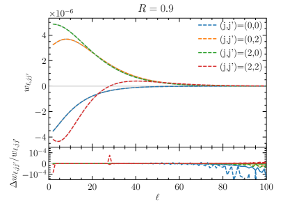
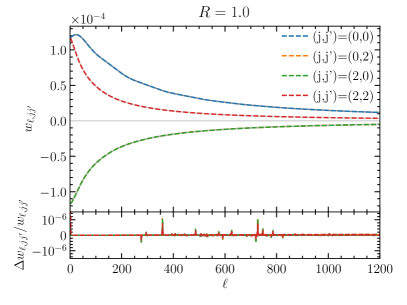
We test the accuracy of our implementation of the 2-FAST algorithm by calculating

$$w_{\ell,jj^{\prime}}(\chi,\chi^{\prime}) =\frac{2}{\pi}\int_{0}^{\infty}\mathrm{d}{}k\,k^{2}\,P(k)\,j_{\ell}^{(j)}(k\chi)\,j_{\ell}^{(j^{\prime})}(k\chi^{\prime})\,,$$ (42)

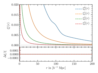
where $j$ and $j^{\prime}$ denote the number of derivatives on the spherical Bessel functions. The functions $w_{\ell,jj^{\prime}}$ appear in the calculation of the angular power spectrum of galaxies in redshift space. In App. G we present the full expression for the angular power spectrum of the redshift-space galaxy distribution, and derive $w_{\ell,jj^{\prime}}$ in terms of $w_{\ell\ell^{\prime}}(\chi,\chi^{\prime})$. We then compare the 2-FAST result with a slow, but accurate computation using the Lucas algorithm Lucas (1995) that we summarize in App. H.

In Fig. 9 we show the comparison with the Lucas algorithm for all values of $(j,j^{\prime})$ needed for linear redshift-space distortion for the $R=1$ ($\chi^{\prime}=\chi$, right panel) and $R=0.9$ ($\chi^{\prime}=0.9\chi$, left panel) cases. The two algorithms agree well and the curves (color curves for 2-FAST, gray curves for Lucas) lie on top of each other at all $\ell$ shown here. The bottom panels of Fig. 9 show that the fractional residuals are $\lesssim\!${10}^{-6}$$ in the case of $R=1$ and $\lesssim\!${10}^{-4}$$ in the case of $R=0.9$ for all $(j,j^{\prime})$ pairs relevant for calculating the linear redshift-space galaxy power spectrum. The one exception is for the $(j,j^{\prime})=(2,2)$ case at the multipole $\ell=2$, where the error is as large as $0.1\text{\,}\mathrm{\char 37\relax}$. A larger sampling number $N$ results in a better match. The differences at small $\ell$ are due to aliasing and can be reduced by choosing a wider integration interval or choosing a different biasing parameter $q$ (see App. B). In Fig. 9 we show the effect of a larger $N$ and a wider integration interval on the residuals as colored solid lines. Some of the glitches in the residuals are likely due to inaccuracy in our implementation of the Lucas algorithm, which we discuss briefly in App. H.

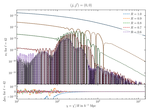
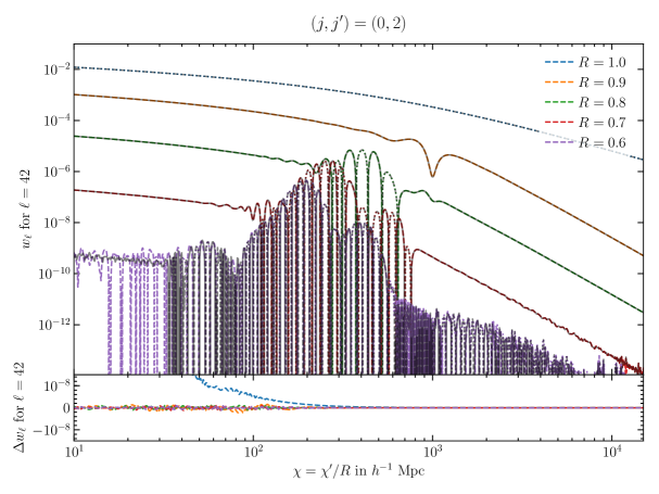
We show a comparison for $w_{\ell=42,jj^{\prime}}(\chi,R\chi)$ as a function of the comoving distance ($\chi$) for different values of $R=1$, $0.9$, $0.8$, $0.7$, $0.6$ in Fig. 10. The curves for the Lucas algorithm are in solid gray for positive values and dashed gray for negative values. The 2-FAST curves are positive for colored dashed lines, and negative for colored dotted lines. The top plot shows the result for $(j,j^{\prime})=(0,0)$ and the bottom plot shows it for $(j,j^{\prime})=(0,2)$. For both plots, we show corresponding residuals between the 2-FAST and Lucas algorithms in the lower panels. Note that here we show the absolute error instead of the relative error because the function $w_{\ell=42,jj^{\prime}}$ frequently crosses zero when $R\neq 1$. The absolute error is generally less than ${10}^{-8}$. The exception is when $R=1.0$ (blue dashed line). However, in that case the relative error is still $<{10}^{-5}$. This can be improved by choosing a wider integration interval $G$ or adopting a smaller biasing parameter $q$ (see App. B).

IV.4 Results: Performance

[b] $N$^a $N_{\chi}$^b. $N_{R}$^c. $\ell_{\mathrm{max}}$ ${}_{2}F_{1,\ell_{\mathrm{max}}}$ $M^{q}_{\ell\ell^{\prime}}$ $C_{\ell}$ Total^d. IO^e 1600 1 1 500 $326\text{\,}\mathrm{ms}$ $215\text{\,}\mathrm{ms}$ $28\text{\,}\mathrm{ms}$ $569\text{\,}\mathrm{ms}$ $68\text{\,}\mathrm{ms}$ 1600 1 1 1200 $393\text{\,}\mathrm{ms}$ $446\text{\,}\mathrm{ms}$ $60\text{\,}\mathrm{ms}$ $899\text{\,}\mathrm{ms}$ $142\text{\,}\mathrm{ms}$ 1600 1600 1 1200 $404\text{\,}\mathrm{ms}$ $453\text{\,}\mathrm{ms}$ $69\text{\,}\mathrm{ms}$ $926\text{\,}\mathrm{ms}$ $163\text{\,}\mathrm{ms}$^f. 3200 3200 5 1200 $3.85\text{\,}\mathrm{s}$ $3.44\text{\,}\mathrm{s}$ $0.45\text{\,}\mathrm{s}$ $7.74\text{\,}\mathrm{s}$ $1.10\text{\,}\mathrm{s}$

Table 1: Performance results.

• Number of sample points on the power spectrum $P(k)$

• Number of redshifts, or number of $\chi$

• Number of ratios $R=\chi^{\prime}/\chi$

• Sum of the three preceding times

• Time spent reading and writing to the disk

• Since we are only interested in compute times here, we did not save all 1600 values to the disk in this case.

We test the performance of our implementation of the 2-FAST algorithm by measuring the time it takes to calculate the angular power spectra in Fig. 9 and Fig. 10, and variations thereof. The result is summarized in Tab. 1 for computing four different scenarios. In the table, $N$ is the number of sampling points on the power spectrum. It defines the size of the FFT array. $N_{\chi}$ is the number of redshifts (comoving radii) we are interested in, $N_{R}$ the number of ratios $R=\chi^{\prime}/\chi$, and $\ell_{\mathrm{max}}$ the maximum multipole moment.

The first two scenarios show that the performance scales roughly proportional to $\ell_{\mathrm{max}}$, which is the total number of multipole moments. The second and third scenarios show that the performance is almost independent of the number of redshifts $N_{\chi}$. The 2-FAST algorithm always calculates the $w_{\ell\ell^{\prime}}(\chi,R\chi)$ at different comoving radii, even when only one redshift is desired, and the FFT takes only a marginal fraction of the total time. This is one of the strengths of the 2-FAST algorithm: one automatically gets $w_{\ell\ell^{\prime}}(\chi,R\chi)$ for all $\chi$ at once.

Finally, the last test scenario demonstrates that the time scales proportionally to the number $N_{R}$ of ratios $R$ and roughly proportionally to the number of sampling points $N$. Hence, it is feasible to create a dense grid of $R$-values to cover a large fraction of the $\chi$-$\chi^{\prime}$ plane. This will be useful, for example, when calculating the angular power spectrum for surveys with a broad radial window function or for weak gravitational lensing convergence.

Note that when we need to calculate the angular harmonic projections of several different power spectra, then the cosmology-independent ${}_{2}F_{1,\ell_{\mathrm{max}}}$ and $M^{q}_{\ell\ell^{\prime}}$ can be precalculated and cached as described in Sec. IV.2. In that case, only the timing from the “$C_{\ell}$” column is relevant.

The 2-FAST method scales with the number of sample points $N$, the number of ratios $N_{R}$, and the number of multipole moments $N_{\ell}$ desired, which we here set as $\ell_{\mathrm{max}}$ (i.e. no binning in multipoles). That is, the time $T$ to take for the calculation scales as

$$T \propto N_{\ell}\cdot N_{R}\cdot N\cdot\log{N}\,.$$ (43)

In our tests, the time for the FFT is negligible compared to other operations that scale with $N$.

We recommend caching the initial value of ${}_{2}F_{1,\ell_{\mathrm{max}}}$ at $\ell_{\mathrm{max}}$. While caching $M_{\ell\ell^{\prime}}^{q}$ may make sense in some cases, the $M_{\ell\ell^{\prime}}^{q}$ cache may demand very large disk space.

V Applications

In this section we consider three applications of the 2-FAST algorithm. First, we study the radial BAO signal, then the lensing potential power spectrum, and finally the lensing-convergence-galaxy cross-correlation. These three test cases demonstrate that we can apply the 2-FAST algorithm for calculating the cross-correlation between two widely separated redshift bins as well as angular autocorrelation and cross-correlation of widely spread-out density fields.

V.1 Radial baryon acoustic oscillations

Figure 11: Projected power spectra with and without BAO. Left: For $\ell=40$. Right: For $\ell=500$. In gray is the BAO power spectrum, in red the power spectrum without BAO; dashed lines indicate negative values. The BAO appears as wiggles for $R\neq 1$, which for larger $\ell$ begin at larger distances.

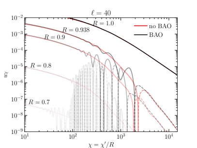
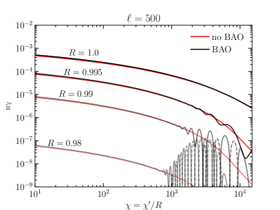
With an accurate and efficient implementation of the 2-FAST algorithm, we study the radial BAO appearing in the harmonic-space correlation function, $w_{\ell}(\chi,R\chi)$:

$$w_{\ell}(\chi,R)=\frac{2}{\pi}\int_{0}^{\infty}\mathrm{d}kk^{2}P(k)j_{\ell}(k\chi)j_{\ell}(kR\chi)\,.$$ (44)

Here we study the harmonic-space correlation function by itself. Summing $w_{\ell}(\chi,\chi^{\prime})$ over $\ell$ corresponds to the real-space two-point correlation function (Lepori et al., 2017) with the wide-angle formula.

In order to highlight the BAO feature, we compare the angular power spectrum $w_{\ell}$ with the $P(k)$ from the CAMB output (with BAO) to the $w_{\ell}$ with the $P(k)$ from the no-BAO fitting formula given by Eisenstein and Hu (1998). We study the radial BAO signature by fixing the multipole moments $\ell$ and the ratio $R$ and plotting $w_{\ell}(\chi,R\chi)$ as a function of comoving radial distance $\chi$.

Fig. 11 shows the comparison for the $w_{\ell=40}$ (left panel) and $w_{\ell=500}$ (right panel) cases. In both panels, the black curves and the red curves show, respectively, the power spectrum with BAO and without BAO. The radial BAO feature is most prominent for $R\neq 1$ cases. Because the acoustic scale of $d_{\mathrm{BAO}}\simeq$106\text{\,}{\mathrm{\text{$h$}}}^{-1}\text{\,}\mathrm{Mpc}$$ is fixed, when fixing the ratio $R$ between two radii, the radial BAO features appear at larger (smaller) radius for larger (smaller) multipole moments that correspond to the smaller (larger) angular scales. That is, for a standard ruler of size $d_{\mathrm{BAO}}$ where radial distance to each end is $\chi$, $\chi^{\prime}=R\chi$, the angle subtended by the ruler is $\cos\theta=[1+R^{2}-(d_{\mathrm{BAO}}/\chi)^{2}]/(2R)$. For small angles one can approximate $\theta\simeq\pi/\ell$, so that $\chi_{\mathrm{BAO}}\simeq d_{\mathrm{BAO}}/\sqrt{(1-R)^{2}+R(\pi/\ell)^{2}}$.

For a randomly oriented ruler of BAO size, the viewing-angle-average projected length is $(\pi/4)d_{\mathrm{BAO}}$, from which we estimate the characteristic radius at which the radial BAO appears as

$$\chi_{\mathrm{BAO}}\simeq\frac{\ell}{4}d_{\mathrm{BAO}}.$$ (45)

The corresponding $R$ is

$$R_{\mathrm{BAO}} \sim 1\pm\frac{\sqrt{16-\pi^{2}}}{\ell}\simeq 1\pm\frac{2.48}{\ell}$$ (46)

to first order in $1/\ell$. For a fiducial $\Lambda$CDM cosmology, we find $\chi_{\mathrm{BAO}}=$1060\text{\,}{\mathrm{\text{$h$}}}^{-1}\text{\,}\mathrm{Mpc}$$, $R_{\mathrm{BAO}}=0.938$ for $\ell=40$ and $\chi_{\mathrm{BAO}}=$13\,250\text{\,}{\mathrm{\text{$h$}}}^{-1}\text{\,}\mathrm{Mpc}$$, $R_{\mathrm{BAO}}=0.995$ for $\ell=500$, which are consistent with Fig. 11.

The result shows that the BAO feature in the angular power spectrum is spread over many multipole moments and distance ratios $R$. As we have shown before, this is because the BAO is a sharp feature defined in the configuration space with a fixed distance scale. Therefore, although we show the radial BAO here as a performance test for the 2-FAST algorithm, the best method of detecting BAO would be to detect in configuration space. After all, one does not need a spherical projection for the BAO, as long as the BAO scale is much smaller than the radial distances to the survey.

V.2 Lensing potential power spectrum

We now turn to the case for the angular power spectrum of a widely spread density distribution using the 2-FAST algorithm. As an example, we calculate the lensing potential power spectrum $C^{\psi\psi}_{\ell}$ for the cosmic microwave background (CMB) lensing, where the source plane is at the CMB’s last-scattering surface ($z_{\star}\simeq 1089$). We denote the comoving angular diameter distance to the surface of last scattering as $\chi_{\star}\equiv\chi(z_{\star})$.

The lensing potential for the CMB lensing is (Lewis and Challinor, 2006)

$$\psi(\hat{\mathbf{n}}) =-2\int_{0}^{\chi_{\star}}\mathrm{d}\chi\,\frac{\chi_{\star}-\chi}{\chi_{\star}\chi}\,\Phi(\chi\hat{\mathbf{n}})\,,$$ (47)

where the gravitational potential $\Phi(\chi\hat{\mathbf{n}})$ is related to the density contrast by Poisson’s equation:

$$k^{2}\Phi(\mathbf{k},a)= \,4\pi Ga^{2}\bar{\rho}_{m}(a)\,\delta_{m}(\mathbf{k},a)$$

$$= \,\frac{3}{2}a^{2}H^{2}\Omega_{m}(a)\,\delta_{m}(\mathbf{k},a)\,.$$ (48)

The angular power spectrum of the lensing potential is then given by

$$C^{\psi\psi}_{\ell} =\int_{0}^{\chi_{\star}}\mathrm{d}\chi\,\varphi(\chi)\,\int_{0}^{\chi_{\star}}\mathrm{d}\chi^{\prime}\,\varphi(\chi^{\prime})\,$$

$$\qquad\times\frac{2}{\pi}\int_{0}^{\infty}\mathrm{d}k\,k^{-2}\,P(k)\,j_{\ell}(k\chi)\,j_{\ell}(k\chi^{\prime})$$ (49)

$$=\int_{0}^{\chi_{\star}}\mathrm{d}\chi\,\varphi(\chi)\,\int_{0}^{\chi_{\star}}\mathrm{d}\chi^{\prime}\,\varphi(\chi^{\prime})\,w_{\ell\ell}^{p}(\chi,\chi^{\prime})\,,$$ (50)

where the index $p=-4$ reminds us that in order to utilize the 2-FAST algorithm as described in Sec. IV, we need to replace the function $P(k)\to k^{-4}P(k)\propto P_{\psi}(k)$. We also defined the radial weighting function $\varphi(\chi)$ as

$$\varphi(\chi) =\frac{\chi_{\star}-\chi}{\chi_{\star}\chi}\,(1+z)\,D(\chi)\,,$$ (51)

where $D(\chi)$ is the linear growth factor. Furthermore, we introduce $R=\chi^{\prime}/\chi$, and we use the symmetry $w_{\ell\ell^{\prime}}(\chi,\chi^{\prime})=w_{\ell^{\prime}\ell}(\chi^{\prime},\chi)$ to find that

$$C^{\psi\psi}_{\ell} =\int_{0}^{1}\mathrm{d}R\,\int_{0}^{\chi_{\star}}\mathrm{d}\ln\chi\,\big{[}2\,\chi^{2}\,\varphi(\chi)\,\varphi(R\chi)\,\big{]}w_{\ell\ell}^{p}(\chi,R)\,.$$ (52)

We first calculate $w_{\ell\ell}^{p}(\chi,R)$ by using the 2-FAST algorithm and perform the integration over $\ln\chi$ and $R$ using the trapezoidal method Press et al. (2007). The sampling in $\ln\chi$ is given by $N$ that we use for FFT in 2-FAST. As shown in Fig. 9, for $\ell\lesssim 100$ the $w_{\ell\ell}(\chi,R)$ are a slowly varying function of $R$, whereas for high $\ell$ they are narrowly peaked around $R\sim 1$. Hence, for $R$ we choose different samplings for $\ell\leq 100$ and $\ell>100$. Specifically, we choose 51 evenly spaced sampling points between $R=1$ and $R=0.9$ for $\ell>100$, and 51 sampling points between $R=1$ and $R=0$ for $\ell\leq 100$. Finally, because the power spectrum is divided by $k^{4}$ compared to the matter density power spectrum, the biasing parameter $q$ also needs to be adjusted to $q\sim-2.5$ (see App. B).

Figure 12: The lensing potential angular power spectrum $C_{\ell}^{\psi\psi}$. In solid black is the result from CAMB, in dashed-dotted black the Limber approximation with $\nu=\ell$ [see Eq. (55)], in dashed black the Limber approximation with $\nu=\ell+0.5$, in dashed gray Limber’s approximation with $\nu=\sqrt{\ell(\ell+1)}$, and in solid green the 2-FAST method presented in this paper. The multiplication by $[\ell(\ell+1)]^{2}$ amplifies the error of the $\nu=\ell$ Limber approximation. Our 2-FAST result is too close to the result from CAMB to be distinguished in this graph.

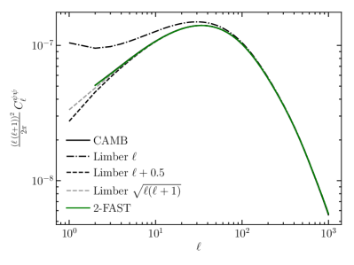
The resulting lensing potential power spectrum is shown in Fig. 12 as a solid green line, which lies on top of the CAMB output (black solid line).

V.2.1 Limber’s approximation

We compare the result with Limber’s approximation (see, for example (Loverde and Afshordi, 2008)), where the spherical Bessel integration is approximated as

$$w_{\ell\ell}(\chi,\chi^{\prime}) =\frac{2}{\pi}\int\mathrm{d}k\,k^{2}\,P(k)\,j_{\ell}(\chi k)\,j_{\ell}(\chi^{\prime}k)$$ (53)

$$\approx\frac{\delta^{D}(\chi-\chi^{\prime})}{\chi^{2}}\,P\left(\frac{\nu}{\chi}\right)\,,$$ (54)

with $\nu=\ell+\frac{1}{2}$. Using Limber’s approximation, the lensing potential $C_{\ell}$ becomes

$$C^{\psi\psi}_{\ell} \approx\int_{0}^{\chi_{\star}}\mathrm{d}\chi\,\frac{\varphi^{2}(\chi)}{\chi^{2}}\,P\left(\frac{\nu}{\chi}\right)\,,$$ (55)

which we integrate using Gauss-Kronrod integration. In the literature, the numerator in the argument to the power spectrum is often approximated as $\nu=\ell$ instead of $\nu=\ell+0.5$. In Fig. 12 we show both for comparison, as well as the exact calculation from the 2-FAST algorithm.

We note that the Limber approximation reproduces the exact calculation for larger multipole moments $\ell\gtrsim 100$, but the result deviates from the exact calculation for larger angular scales. In particular, the “old” Limber approximation with $\nu=\ell$ shows the largest deviation, whereas the proper Limber approximation with $\nu=\ell+0.5$ as derived in Loverde and Afshordi (2008) follows the correct value to the larger scales $\ell\simeq 10$. We note that a further improvement can be achieved by using $\nu=\sqrt{\ell(\ell+1)}$ (gray dashed line), which was already hinted at in (Loverde and Afshordi, 2008).

V.3 Lensing convergence-galaxy cross correlation

Figure 13: The two terms contributing to Eq. (58): $jj^{\prime}=00$ on the left and $jj^{\prime}=02$ on the right. In addition to our 2-FAST method, we show three versions of the Limber approximation, which are defined as in Fig. 12. The gray bands show the estimated error due to the discrete sampling of $R^{\prime}=\chi/\chi^{\prime}$. For large $\ell$, the Limber approximation agrees well with the more exact 2-FAST calculation. However, at $\ell\lesssim 10$, none of the Limber approximations achieves better than percent-level precision.

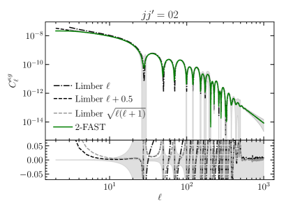
As a final test case, we calculate the cross-correlation $C^{\kappa g}_{\ell}$ between foreground galaxies at comoving distance $\chi^{\prime}$ (redshift $z^{\prime}$) and the lensing convergence field $\kappa$ reconstructed from the source galaxies at distance $\chi_{\star}$ (redshift $z_{\star}$). Such a cross-correlation dominates the cross-correlation between galaxies widely separated in redshift, because the lensing magnification traces the line-of-sight directional convergence.

Besides the relativistic corrections (see Jeong and Schmidt (2015) for a review), the dominant components of the observed galaxy density contrast $\delta_{g}$ of galaxies are given by

$$\delta_{g}(\mathbf{k}) =[b_{g}+f(\hat{\mathbf{n}}\cdot\hat{\mathbf{k}})^{2}]\,\delta_{m}(\mathbf{k})+2(\mathcal{Q}-1)\kappa\,,$$ (56)

where $b_{g}$ is the galaxy bias, $f$ the linear growth rate $f\equiv\mathrm{d}\ln D/\mathrm{d}\ln a$, $\delta_{m}(\mathbf{k})$ the matter density contrast, $\mathcal{Q}$ the slope of the luminosity function at the survey limit, and $\kappa$ is the lensing convergence. Here, we neglect the factor $2(\mathcal{Q}-1)$ and we set $b_{g}=1$, as those factors are specific to the galaxies and survey.

The lensing convergence is given by

$$\kappa(\chi\hat{\mathbf{n}}) =-\tfrac{1}{2}\nabla_{\theta}^{2}\psi(\hat{\mathbf{n}})\,,$$ (57)

where the lensing potential $\psi(\hat{\mathbf{n}})$ is given in Eq. (47). Then, the cross-correlation between lensing convergence for the sources at distance $\chi_{\star}$ and galaxies at distance $\chi^{\prime}$ is given by Jeong et al. (2009)

$$C^{\kappa g}_{\ell}(\chi_{\star},\chi^{\prime}) =\tfrac{3}{2}\Omega_{m}H_{0}^{2}\,\ell(\ell+1)\int_{0}^{\chi_{\star}}\frac{d\chi}{\chi}\,\frac{\chi_{\star}-\chi}{\chi_{\star}}$$

$$\qquad\times\frac{D(z)D(z^{\prime})}{a}$$

$$\qquad\times\big{[}b^{\prime}w^{p}_{\ell,00}(\chi,\chi^{\prime})-f^{\prime}w^{p}_{\ell,02}(\chi,\chi^{\prime})\big{]}\,,$$ (58)

where we attach the suffix $p=-2$ to $w_{\ell,jj^{\prime}}$ to signify that the biased power spectrum $k^{-2}P(k)$ is to be used. To use the 2-FAST algorithm, it is advantageous to exploit the symmetry $w_{\ell,jj^{\prime}}(\chi,\chi^{\prime})=w_{\ell,j^{\prime}j}(\chi^{\prime},\chi)$ and introduce $R^{\prime}=\chi/\chi^{\prime}$. That is,

$$w^{p}_{\ell,jj^{\prime}}(\chi,\chi^{\prime}) =w^{p}_{\ell,j^{\prime}j}(\chi^{\prime},R^{\prime}\chi^{\prime})\,.$$ (59)

This way we can keep $\chi^{\prime}=\mathrm{const}$ while performing the integral over $R^{\prime}$. With $\ln\chi=\ln{R^{\prime}}+\ln{\chi^{\prime}}$ we get

$$C^{\kappa g}_{\ell}(\chi_{\star},\chi^{\prime}) =\tfrac{3}{2}\Omega_{m}H_{0}^{2}\,\ell(\ell+1)\int_{0}^{\chi_{\star}/\chi^{\prime}}d\ln{R^{\prime}}\,\frac{\chi_{\star}-\chi}{\chi_{\star}}$$

$$\qquad\times\frac{D(z)D(z^{\prime})}{a}$$

$$\qquad\times\big{[}b^{\prime}w^{p}_{\ell,00}(\chi^{\prime},R^{\prime}\chi^{\prime})-f^{\prime}w^{p}_{\ell,20}(\chi^{\prime},R^{\prime}\chi^{\prime})\big{]}\,.$$ (60)

We partition the range in $\ell$ into four intervals. In each interval we choose a different sampling for $\ln{R^{\prime}}$. This is needed, since the integrand is broad at low $\ell$, but becomes a narrowly peaked function at high $\ell$. Specifically, for our test case $z^{\prime}=0.3$ ($\chi^{\prime}=$835\text{\,}{\mathrm{\text{$h$}}}^{-1}\text{\,}\mathrm{Mpc}$$), $z_{\star}=2.2$ ($\chi_{\star}=$3796\text{\,}{\mathrm{\text{$h$}}}^{-1}\text{\,}\mathrm{Mpc}$$) we found the following choices to work well for the integer values $m$:

$\ell$-interval		$R^{\prime}$	$m$
500$\,\rightarrow\,$	1000	$\,e^{0.0001\,m}$	$-400,\ldots,400$
200$\,\rightarrow\,$	499	$\,e^{0.0005\,m}$	$-200,\ldots,200$
30$\,\rightarrow\,$	199	$\,e^{0.002\,m}$	$-400,\ldots,200$
2$\,\rightarrow\,$	29	$\,e^{0.01\,m}$	$-300,\ldots,151$

These choices ensure an accurate calculation of all the terms in Eq. (60). However, since Eq. (60) is dominated by the $(j,j^{\prime})=(0,0)$ term, a less dense grid in $R^{\prime}$ may be sufficient for many applications. We then integrate using the trapezoidal method. Here, we use $q=0.5$ (App. B).

When either $z^{\prime}$ or $z_{\star}$ differs from its values investigated here, then the values for $R$ in the table above may be used as a starting point, and for each $\ell$ region one may increase the interval in $R$, as well as the number of sampling points in $R$ until convergence is reached.

Alternatively, one can avoid the somewhat ad hoc choice of $R$-sampling by integrating $M_{\ell\ell^{\prime}}(t,R)$ over the radial window function as shown in Eq. (37). While we have not further investigated here, Assassi et al. (2017) have shown that the integration can be done with the hypergeometric function ${}_{3}F_{2}$ if the radial function can be approximated by a sum of polynomials. We shall further study this in future publications.

V.3.1 Comparison

Figure 14: The lensing-convergence-galaxy cross-correlation Eq. (58), the sum of the two plots in Fig. 13. All labels have the same meaning as in that figure. The $jj^{\prime}=00$ term dominates the cross-correlation.

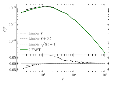
In this section we compare our results with several versions of Limber’s approximation. To be applicable to the $w_{\ell,02}$ term in Eq. (58), we extend Limber’s approximation to include the cases $\ell\neq\ell^{\prime}$ by using the results from Loverde and Afshordi (2008). We defer the details of this derivation to App. I.

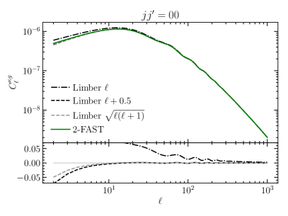
Fig. 13 and Fig. 14 show the comparison of the 2-FAST calculation with three versions of Limber’s approximation. Fig. 13 shows the two terms in Eq. (58) separately in the left and right panels, whereas Fig. 14 shows the full lensing-convergence-galaxy cross-correlation power spectrum. In both figures the estimated error due to discretization of the $R^{\prime}$-integral is shown as a gray band around the 2-FAST line. Also shown in the lower panels of the figures is the relative difference of Limber’s approximation to the 2-FAST algorithm calculation.

Again, Limber’s approximation is accurate for larger multipole moments, but deviates from the exact calculation from 2-FAST on small multipoles (larger angular scales). However, we note that as in Sec. V.2.1, the $\nu=\sqrt{\ell(\ell+1)}$ version of Limber’s approximation agrees quite well with the 2-FAST results. Percent-level precision is achieved with this version of Limber’s approximation for $\ell\gtrsim 10$.

VI Conclusion

In this paper, we have presented the 2-FAST algorithm for projecting the three-dimensional power spectrum onto two-point correlation functions in configuration space as well as in spherical harmonic space. Based on the FFTLog method in Talman (1978); Siegman (1977); Hamilton (2000), we generalize to the case $\ell\neq\ell^{\prime}$.

By decomposing the power spectrum with FFTLog basis functions and the coefficients $\phi^{q}$, the infinite-range integrations in the 2-FAST algorithm are done as gamma functions and Gauss hypergeometric functions ${}_{2}F_{1}$ for, respectively, calculating $\xi_{\ell}^{\nu}(r)$ and $w_{\ell\ell^{\prime}}(\chi,\chi^{\prime})$. Therefore, 2-FAST bypasses the difficulties in dealing with oscillatory spherical Bessel functions with large arguments. At the core of the 2-FAST algorithm is a recursion algorithm for computing the Gauss hypergeometric function. In particular, the stable backward recursion enables a fast, high-precision calculation of $w_{\ell\ell^{\prime}}(\chi,\chi^{\prime})$.

Using the fast Fourier transformation, the 2-FAST algorithm calculates the $w_{\ell\ell^{\prime}}(\chi,R\chi)$ for multiple values of $\chi$ (regularly spaced in the logarithmic interval) by one operation of FFT. In addition, an efficient recursion along the $\ell$-direction provides $w_{\ell\ell^{\prime}}(\chi,R\chi)$ essentially to arbitrary $\ell$ and $\ell^{\prime}$ values (although the current implementation is done for $\Delta\ell=\pm 4$, the extension is trivial, if necessary). Furthermore, we can then easily map out $w_{\ell\ell^{\prime}}(\chi,\chi^{\prime})$ in the $\chi$-$\chi^{\prime}$ plane by repeating the procedure for different values of $R$.

From the transformation matrix from $P(k)$ to $C_{\ell}$ in Sec. IV.2 and the two examples in Sec. V.2 and Sec. V.3, we have demonstrated that Limber’s approximation with the identification $k=\sqrt{\ell(\ell+1)}/\chi$ performs far better than the traditional prescription of $k=\ell/\chi$ or $k=(\ell+\frac{1}{2})/\chi$, and it reaches down to $\ell=10$ for the convergence-galaxy cross-correlation power spectrum. For small-angle galaxy surveys, using this improved Limber approximation may suffice. For the future galaxy surveys with large angular footprints, however, we need to use the full calculation, and the 2-FAST algorithm will make it fast and accurate.

There are two directions in which we can extend the 2-FAST algorithm. First, we can boost the speed of integration over the survey radial window function by approximating the window function as a sum over polynomials. In this case, the integration over a polynomial window function can be done as a hypergeometric function ${}_{3}F_{2}$ Assassi et al. (2017), and a detailed study of recursion can accelerate the calculation faster than the current 2-FAST method that integrates over the precalculated $w_{\ell\ell^{\prime}}(\chi,\chi^{\prime})$ on the $\chi-\chi^{\prime}$ space. Second, for the $n$th-order angular polyspectra, we need to calculate the overlapping integration of $n$ spherical Bessel functions with some polynomial. We surmise that the Fourier-based method that we presented here can aid greatly in this type of calculation as well. These two issues must be addressed to fully exploit the large angular scale galaxy clustering signatures from future galaxy surveys.

The Julia version of the 2-FAST implementation can be obtained from https://github.com/hsgg/twoFAST. The authors have a plan to implement the FORTRAN and C versions in the future.

Appendix A Discrete versions of the algorithm

In the main text, we discuss the 2-FAST algorithm based on the integration of continuous functions over an infinite range. In this appendix, we shall give discrete versions of the relevant equations that we used when implementing the algorithm. First, we present the equations for the FFTLog transformation of the biased power spectrum that we have implemented through the fast Fourier Transformation of the array spaced with a constant logarithmic interval (App. A.1). We then show the discrete version for calculation of $\xi_{\ell}^{\nu}(r)$ (App. A.2) and $w_{\ell\ell^{\prime}}(\chi,\chi^{\prime})$ (App. A.3). Finally, we shall present some basic equations appearing commonly for all cases and clarify the relation between variables.

A.1 FFT of biased power spectrum

Here we derive the discrete version of Eq. (6). We define

$$x_{m} =m\frac{L}{N} \kappa_{n} =n\,\frac{2\pi}{L}$$ (61)

where $N$ is the number of sample points, $L$ is the size of the interval, and $n,m=0,\ldots,N-1$. Then Eq. (6) becomes

$$\phi^{q}(x_{m}) =\frac{1}{L}\sum_{n}e^{i2\pi nm/N}\,e^{(3-q)\kappa_{n}}\,P(k_{0}e^{\kappa_{n}})$$ (62)

$$=\frac{1}{L}\,\Big{\{}\mathrm{RFFT}\big{[}e^{(3-q)\kappa_{n}}\,P(k_{0}e^{\kappa_{n}})\big{]}\Big{\}}^{*}$$ (63)

where “RFFT” denotes the fast Fourier Transform specialized for a real function, and the ^∗ symbol denotes complex conjugation.

To reduce ringing we avoid sharp edges at the interval boundaries by applying the same window function as Eq. (C.1) in McEwen et al. (2016). We repeat it here for completeness:

$$W(x) =\begin{cases}\frac{x-x_{\mathrm{min}}}{x_{\text{left}}-x_{\mathrm{min}}}-\frac{1}{2\pi}\sin\left(2\pi\,\frac{x-x_{\mathrm{min}}}{x_{\text{left}}-x_{\mathrm{min}}}\right),&x<x_{\text{left}}\\ 1,&x_{\text{left}}<x<x_{\text{right}}\\ \frac{x_{\mathrm{max}}-x}{x_{\mathrm{max}}-x_{\text{right}}}-\frac{1}{2\pi}\sin\left(2\pi\,\frac{x_{\mathrm{max}}-x}{x_{\mathrm{max}}-x_{\text{right}}}\right),&x>x_{\text{right}}\end{cases}$$ (64)

We apply this window function to the biased power spectrum both before and after Fourier transforming.

A.2 Discrete version of single Bessel function transform

Here we give a discrete version of Eq. (15). Let $G$ be the size of the logarithmic integration interval, and $N$ the number of sample points. Eq. (15) with $t_{m}=2\pi m/G$ and $\rho_{n}=nG/N$ then becomes

$$\xi^{\nu}_{\ell}(r_{n}) =\frac{k_{0}^{3}e^{-(q_{\nu}+\nu)\rho_{n}}}{\pi\alpha^{\nu}G}\sum_{m}e^{i2\pi mn/N}\,\phi^{q_{\nu}+\nu}(t_{m})\,M^{q_{\nu}}_{\ell}(t_{m})$$ (65)

$$=\frac{k_{0}^{3}e^{-(q_{\nu}+\nu)\rho_{n}}}{\pi\alpha^{\nu}G}\,\mathrm{BRFFT}\big{[}\phi^{q_{\nu}+\nu}(t_{m})\,M^{q_{\nu}}_{\ell}(t_{m})\big{]}$$ (66)

where $\mathrm{BRFFT}[\tilde{f}(x_{m})]=G\times\mathrm{IRFFT}[\tilde{f}(x_{m})]$ is the inverse transform of a real function $f(x)$ without dividing by $G$.

A.3 Discrete version of two Bessel function transform

Here we give a discrete version of Eq. (29). With $t_{m}=2\pi m/G$ for $N$ samples over an interval $G$, and $\rho_{n}=nG/N$ we get

$$w_{\ell\ell^{\prime}}(\chi_{n},R) =4k_{0}^{3}\,\left(\frac{\chi_{n}}{\chi_{0}}\right)^{-q}\frac{1}{G}\sum_{m}e^{i2\pi nm/M}\,\phi^{q}(t_{m})\,M^{q}_{\ell\ell^{\prime}}(t_{m},R)$$

$$=\frac{4k_{0}^{3}}{G}\,\left(\frac{\chi_{n}}{\chi_{0}}\right)^{-q}\,\mathrm{BRFFT}\big{[}\phi^{q}(t_{m})\,M^{q}_{\ell\ell^{\prime}}(t_{m},R)\big{]}$$ (67)

where $\mathrm{BRFFT}[\tilde{f}(x_{m})]=G\times\mathrm{IRFFT}[\tilde{f}(x_{m})]$ is the inverse transform of a real function $f(x)$ without dividing by $G$.

A.4 Relation between variables

Since the $t_{m}$ arguments to $\phi^{q}$ and $M^{\nu,q}_{\ell}$ [Eq. (15)], or $\phi^{q}$ and $M^{q}_{\ell\ell^{\prime}}$ [Eq. (29)] are identical, we have

$$x_{m} =m\,\frac{L}{N}=t_{m}=m\,\frac{2\pi}{G}$$ (68)

Thus,

$$G =\frac{2\pi N}{L}=\ln\bigg{(}\frac{k_{\mathrm{max}}}{k_{\mathrm{min}}}\bigg{)}$$ (69)

where the last equality follows from the choice $k_{0}=k_{\mathrm{min}}$, using the second of Eq. (61), and by writing the first of Eq. (26) [or Eq. (12)] for $k_{\mathrm{max}}$ as

$$\frac{k_{\mathrm{max}}}{k_{\mathrm{min}}} =e^{2\pi N/L}$$ (70)

Finally, from our discretization of $\rho_{n}$ above, Eq. (26) becomes

$$\chi_{n} =\chi_{0}\,e^{nG/N}$$ (71)

This also holds for Eq. (12) when $\chi\rightarrow r$.

Appendix B On the choice of $N$, $G$, and the biasing parameter $q$

In this appendix, we study the effect of different biasing parameters $q$ and the resolution $N$ and interval $G$ of the FFTLog transformation. For the continuous FFTLog transformation, $q$ is only constrained by Eq. (10), Eq. (20) and Eq. (32), which together constitute the requirement that the integrals converge. When we implement FFTLog as a discrete Fourier transformation, however, numerical artifacts affect the accuracy of the result, and the error depends sensitively on different choices of the parameters $q$, $N$ and $G$. There are three types of numerical error involved in the Fourier transformation: (A) ringing, which is the loss of high-frequency modes, is minimized by avoiding sharp edges in the power spectrum; (B) aliasing, due to limited sampling, can be reduced by increasing the number of sampling points $N$; (C) wrap-around, due to the FFT assuming periodic data so that the high-$k$ modes influence the low-$k$ modes, is mitigated via zero-padding.

In particular, it turns out that the accuracy of the 2-FAST algorithm depends sensitively on the choice of the biasing parameter $q$. We used $q=1.9$ for calculating $\xi_{\ell}^{\nu}(r)$ and $q=1.1$ for calculating $w_{\ell\ell^{\prime}}(\chi,\chi^{\prime})$. When integrating the overlapping of two spherical Bessel functions with $k^{-2}P(k)$ (galaxy-lensing cross power spectrum, Sec. V.3) and $k^{-4}P(k)$ (lensing potential power spectrum, Sec. V.2), we use, respectively, $q=0.5$ and $q=-2.5$. In this section, we systematically study these choices of the parameter $q$.

We implement Eq. (15) and Eq. (29) by the 2-FAST algorithm as follows: we first calculate $\phi^{q}(t)$ by using the discrete FFTLog and then multiply it by the analytically calculated $M_{\ell}^{q_{\nu}}(t,R)$ or $M_{\ell\ell^{\prime}}^{q}(t,R)$. We then apply the FFTLog again to calculate $\xi_{\ell}^{\nu}(r)$ or $w_{\ell\ell^{\prime}}(\chi,R)$. In this procedure, there are two aliasing effects that worsen the accuracy of the 2-FAST algorithm: the aliasing effect associated with the calculation of $\phi^{q}(t)$, and the aliasing effect associated with the backward-FFTLog for the convolution. Of course, we can remedy the aliasing effects by reducing the sampling intervals $\Delta_{k}=G/N$ and $\Delta_{t}=2\pi/G$, respectively, in the wave number space and its dual space. We find that, however, it is more efficient to reduce the aliasing effect by choosing an appropriate biasing parameter $q$. We study the two aliasing effects in the following subsections.

B.1 Aliasing effect in FFTLog of $P(k)$

Figure 15: The Fourier-space function $|\phi^{q}(t)|$ for five different numbers of samplings $N=128,~{}256,~{}512,~{}1024,~{}10000$ for each biasing paramter $q=0,1,2,3$. The insets show the full spectrum; the main panels are zoom-ins. The dropoff of the respective maximum $t$ for each $N$ is due to the application of the window function after the FFTLog transform. Aliasing is strongest for the $q=0$ case. The features in the spectrum are captured by $N\gtrsim 512$, though we choose $N=1024$. Here we used the interval $k_{\mathrm{min}}=${10}^{-5}\text{\,}\mathrm{\text{$h$}}\text{\,}{\mathrm{Mpc}}^{-1}$$ to $k_{\mathrm{max}}=${10}^{3}\text{\,}\mathrm{\text{$h$}}\text{\,}{\mathrm{Mpc}}^{-1}$$.

Figure 16: The result of the 2-FAST algorithm for $\xi(r)$ (left) and its second derivative (right) for several choices of the sampling number $N$. For $\xi(r)$ itself, percent-level precision is achieved with $N\geq 256$. The second derivative is noisier as it depends on smaller structure in the power spectrum, and so it achieves percent-level precision with $N\geq 512$. (The differences at $r\gtrsim$150\text{\,}{\mathrm{\text{$h$}}}^{-1}\text{\,}\mathrm{Mpc}$$ are likely due to pathologies in the quadosc algorithm as shown in Fig. 4.)

Figure 17: Here we show the behavior of the method as it depends on the number of sample points $N$ in the interval $k_{\mathrm{min}}=${10}^{-5}\text{\,}\mathrm{\text{$h$}}\text{\,}{\mathrm{Mpc}}^{-1}$$ to $k_{\mathrm{max}}=${10}^{5}\text{\,}\mathrm{\text{$h$}}\text{\,}{\mathrm{Mpc}}^{-1}$$ for a power spectrum with BAO (left) and a power spectrum without BAO (right) at $\chi=\chi^{\prime}=$2370\text{\,}{\mathrm{\text{$h$}}}^{-1}\text{\,}\mathrm{Mpc}$$. In each graph, the top panel shows the power spectrum, and the bottom panel shows the residual to the 2-FAST method with $N=2048$. Left: Using a power spectrum with BAO. If the number of sampling points is below $N\sim 128$, nearly all of the BAO features are missed, and show up in the residuals. At $N=128$, the BAO feature is missed only at $\ell\gtrsim 500$. This is due to the logarithmic spacing of the sample points $k_{n}$ of the power spectrum $P(k_{n})$, since for larger $\ell$, most of the power comes from larger $k$, where the sample points are more sparse. Right: For a power spectrum without BAO. In this case even $N=32$ sampling points capture much of the structure of the power spectrum.

Figure 18: Top left: The absolute value (top panel) and the complex phase angle (bottom panel) of $M^{q_{\nu}}_{\ell}(t)$ as a function of the integration parameter $t$. Note that the absolute value is quite featureless and merely rises or decays somewhat. Top right: The same but for $M^{q}_{\ell\ell^{\prime}}(t,R)$ as needed for the integral over two spherical Bessel functions. Bottom left: Here we show the absolute value and the complex phase angle of the full integrand in Eq. (15) for $\nu=0$. Bottom right: The same but for two spherical Bessel functions Eq. (29), using the biased power spectrum $k^{p}\,P(k)$.

Figure 19: The function $\xi_{\ell}^{\nu}(r)$ for $\nu=0,1,2,3$ and for $\ell=0$ (top left), $\ell=1$ (top right), $\ell=2$ (bottom left), and $\ell=4$ (bottom right) as calculated using $q_{\nu}$ described in App. B. We also show the relative residuals to the quadosc algorithm.

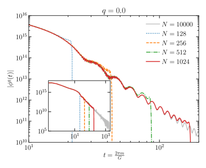
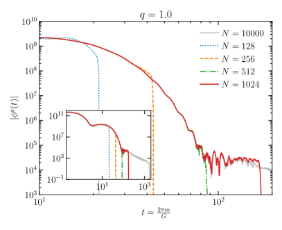
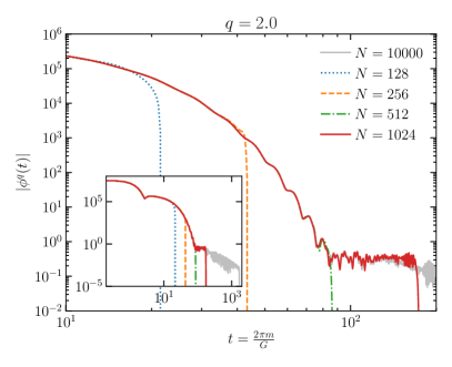
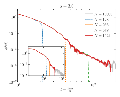
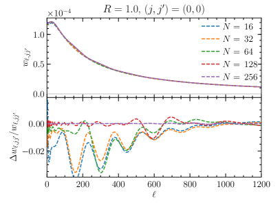
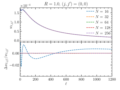
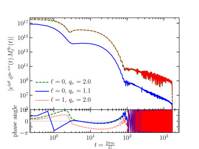
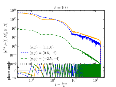
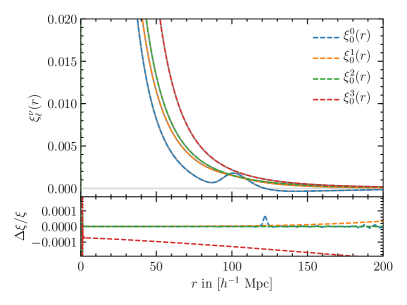
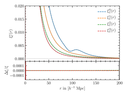
In Fig. 15 we show the dependence of $\phi^{q}(t)$ on the biasing parameter $q$ and the number of sampling points $N$ for a given integration interval $k_{\mathrm{min}}=${10}^{-5}\text{\,}\mathrm{\text{$h$}}\text{\,}{\mathrm{Mpc}}^{-1}$$ and $k_{\mathrm{max}}=${10}^{3}\text{\,}\mathrm{\text{$h$}}\text{\,}{\mathrm{Mpc}}^{-1}$$. For all four biasing parameters ($q=0$, $1$, $2$, and $3$ from top left to bottom right), we calculate $\phi^{q}(t)$ with four different resolutions ($N=1024$, $N=512$, $N=256$, and $N=128$) to compare with the benchmark case with $N=10000$ (gray line). As all the other conditions are the same, any differences from the benchmark case must be due to aliasing. As expected, the aliasing effects show up near the Nyquist frequency ($t_{\mathrm{Ny}}\simeq N\pi/G$, corresponding to the cutoff) for each case. Among the cases that we study here, the aliasing effect is largest for the $q=0$ case and smaller for cases with larger $q$ ($q=2$ and $q=3$), where the biasing makes the lower-$k$ slope (wave number smaller than the turnover wave number $k_{\mathrm{to}}\sim$0.01\text{\,}\mathrm{\text{$h$}}\text{\,}{\mathrm{Mpc}}^{-1}$$) shallower.

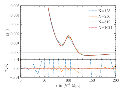
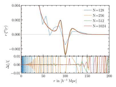
As for $N$, we need to choose the grid size $N$ large enough so that the FFTLog sampling captures the BAO features correctly. In Fig. 16, we show the dependence of $\xi(r)$ and its second derivative on $N$. Since the second derivative depends on smaller-scale structure in the function $P(k)$, it weights larger $t$ in Fourier space [$\phi^{q}(t)$] more heavily, and a higher sampling number $N$ is needed to achieve the same precision as for $\xi(r)$. We also show the dependence of $w_{\ell\ell}(\chi,\chi)$ on $N$ in Fig. 17 for a power spectrum with BAO (left) and a power spectrum without BAO (right). As shown from the BAO-less calculation (right panel), the broad shape is well reproduced even for a very small sampling number $N\sim 32$. The BAO feature, however, is not completely recovered for the sparse sampling ($N<512$) cases (see, for example, Fig. 2).

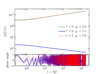
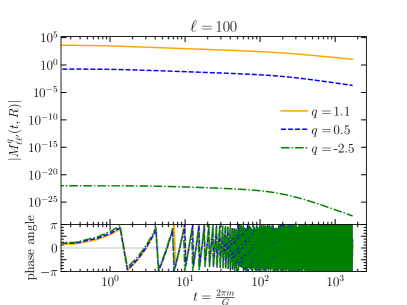
The top two panels of Fig. 18 show the functions $M^{q_{\nu}}_{\ell}(t)$ (left) and $M^{q}_{\ell\ell^{\prime}}(t,R)$ (right). In each graph the top panel shows the absolute values, and the bottom panel shows the phase angle of the complex number. The absolute value rises or falls monotonically depending on the value of $q$, as shown in the figure. The bottom two panels of Fig. 18 show the full integrands of the integrals in Eq. (15) (left) and Eq. (29) (right). Note that for the right figure (for two spherical Bessel functions), we used the biased power spectrum $k^{p}\,P(k)$ as introduced in the main text. Note that in all cases the full integrand decreases rapidly with $t$ for the choices of $q$ shown.

Finally, we checked the prescription that we have adopted in Sec. III: As a default, we choose $q_{\nu}=1.9-\nu$ as long as it is within the allowed range given in Eq. (20). If the mean results in a $q_{\nu}$ outside the range, then we use instead

$$q_{\nu} =\frac{1}{3}(q_{\nu,\mathrm{min}}+2q_{\nu,\mathrm{max}})\,,$$ (72)

where $q_{\nu,\mathrm{min}}$ and $q_{\nu,\mathrm{max}}$ are the boundaries given in Eq. (20). In Fig. 19 we verify that the resulting $\xi_{\ell}^{\nu}(r)$ from this choice of $q_{\nu}$ matches well with the benchmark results from the quadosc calculation.

B.2 Aliasing effect in backward FFTLog

Figure 20: Here we exemplify the dependence of the result of the 2-FAST algorithm for $w_{\ell\ell}(\chi,\chi)$ on the integration interval $G$ for $\ell=42$ and $q=1.9$. The ratio $G/N$ is kept constant so that the same sampling points on the power spectrum are used in all cases. The black line is the result from the Lucas algorithm. While the error goes down for larger $G$, even extremely large ranges $G$ lead to significant error for $\chi<$100\text{\,}{\mathrm{\text{$h$}}}^{-1}\text{\,}\mathrm{Mpc}$$. The error here is dominated by the $s>0$ terms. To get correct results it is more efficient to adjust $q$.

Figure 21: The dependence of the 2-FAST result for $w_{\ell\ell}(\chi,R\chi)$ on the choice of $q$ for $\ell=42$ and $R=1$ (left) and $0.8$ (right). For $R=1$, choosing $q\lesssim 1.5$ is required to get an accurate result for the cosmologically relevant range $\chi\gtrsim$100\text{\,}{\mathrm{\text{$h$}}}^{-1}\text{\,}\mathrm{Mpc}$$. In contrast, for $R=0.8$, the aliasing effect in relevant scales is small for all values of $q$ shown here.

Figure 22: Same as Fig. 21, except that $\ell=1000$ and $R=1,~{}0.99$. Once again, for $R=1$, $q=1.1$ results in a small aliasing effect. For $R=0.99$, any value $q\lesssim 1.5$ gives a small aliasing effect over the cosmologically relevant scale.

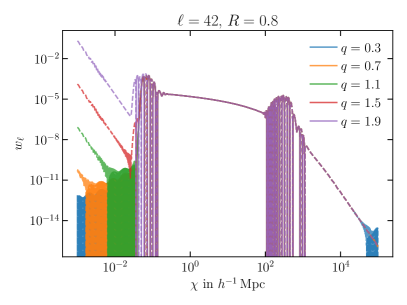
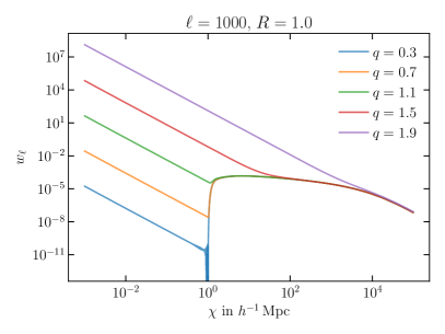
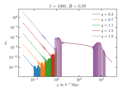
When implementing the 2-FAST algorithm, we calculate the convolution between the power spectrum $P(k)$ and one or two spherical Bessel functions by the backward discrete FFTLog transformation of $\phi^{q}(t)M_{\ell}^{q_{\nu}}(t)$ or $\phi^{q}(t)M_{\ell\ell^{\prime}}^{q}(t,R)$, which are, respectively, the analytically calculated Fourier transformations of one or two spherical Bessel functions. In this section, we study yet another aliasing effect associated with the discrete sampling in $t$ space and justify our choice of the biasing parameter $q$.

To avoid clutter, let us consider calculating the following convolution integral:

$$f(x)=\int_{-\infty}^{\infty}\mathrm{d}y\,g(y)\,h(x+y)=\int_{-\infty}^{\infty}\frac{\mathrm{d}q}{2\pi}\,\tilde{g}(-q)\,\tilde{h}(q)\,e^{iqx},$$ (73)

where $\tilde{g}(q)$ and $\tilde{h}(q)$ are the functions in Fourier space. In order to mock the 2-FAST implementation, we discretize the later integration as well as the calculation of $\tilde{g}$ by using $N$ sampling points within the $x$-range of $G$. First, the Fourier transformation of $g(x)$ is

$$\tilde{g}(q_{m})=\Delta_{x}\sum_{k=0}^{N-1}g(x_{k})\,e^{-ix_{k}q_{m}}=\frac{G}{N}\sum_{k=0}^{N-1}g(x_{k})\,e^{-i2\pi mx_{k}/G},$$ (74)

where $q_{m}=m\Delta_{q}$ and $x_{k}=k\Delta_{x}$ with the intervals $\Delta_{x}\equiv G/N$ and $\Delta_{q}\equiv 2\pi/G$ in $x$ space and $q$ space. On the other hand, the function $\tilde{h}(q)$ is calculated from the Fourier transformation:

$$\tilde{h}(q)=\int_{-\infty}^{\infty}\mathrm{d}x\,h(x)\,e^{-iqx}\,.$$ (75)

Combining the two, we find that the implementation actually calculates

$$f(x_{n}) =\frac{1}{G}\sum_{m=0}^{N-1}\,e^{iq_{m}x_{n}}\tilde{g}(-q_{m})\,\tilde{h}(q_{m})=\sum_{k=0}^{N-1}g(x_{k})\int_{-\infty}^{\infty}\mathrm{d}x\,h(x)\left[\frac{1}{N}\sum_{m=0}^{N-1}e^{i2\pi m\;\!\left(x_{n}+x_{k}-x\right)/G}\right]\,.$$ (76)

Here, the function in square brackets,

$$W(x)\equiv\frac{1}{N}\sum_{m=0}^{N-1}e^{i2\pi mx/G}=e^{i\pi\frac{N-1}{G}x}\,\frac{\sin(N\pi x/G)}{N\sin(\pi x/G)},$$ (77)

can be approximated as

$$W(x)\simeq\frac{G}{N}\sum_{s=-\infty}^{\infty}\delta^{D}(x+sG)\,,$$ (78)

which is exact in the $N\to\infty$ limit. With this approximation, we find that the convolution integral Eq. (76) becomes

$$f(x_{n}) \simeq\Delta_{x}\sum_{k=0}^{N-1}g(x_{k})\sum_{s=-\infty}^{\infty}h(x_{n}+x_{k}+sG)\,,$$ (79)

where $\Delta_{x}=G/N$, $x_{n}=n\Delta_{x}$, and $x_{k}=k\Delta_{x}$. Comparing Eq. (73) with Eq. (79), we see that the desired convolution corresponds to the $s=0$ case, and all the other $s$ values cause aliasing. Note that the $s\neq 0$ peaks are separated by $2\pi/\Delta_{q}=G$, that is, the total duration of discrete sampling in $x$ space. In order to suppress this effect, we need to employ a function $h(x)$ that decays fast so that the aliasing contribution is far smaller than the desired result at $s=0$.

For the case at hand, $g(\kappa)=e^{(3-q)\kappa}P(k_{0}e^{\kappa})$ is the biased power spectrum, and $h(\kappa)=e^{q_{\nu}\kappa}j_{\ell}(\alpha e^{\kappa})$, Eq. (13), and $h(\kappa)=e^{q\kappa}j_{\ell}(\alpha e^{\kappa})j_{\ell^{\prime}}(R\alpha e^{\kappa})$, Eq. (27), for calculating, respectively, $\xi_{\ell}^{\nu}(r)$ and $w_{\ell\ell^{\prime}}(\chi,\chi^{\prime})$. The outcomes of the 2-FAST implementation are then

$$\xi_{\ell}^{\nu}(r) =\frac{k_{0}^{3}e^{-(q_{\nu}+\nu)\rho}}{2\pi^{2}(k_{0}r_{0})^{\nu}}\,\Delta_{\kappa}\sum_{k}e^{(3-q_{\nu}-\nu)\kappa}P(k)\sum_{s=-\infty}^{\infty}e^{q_{\nu}(\kappa+\rho+sG)}\,j_{\ell}(kre^{sG})$$ (80)

$$=\frac{\Delta_{\kappa}}{2\pi^{2}}\sum_{k}\frac{k^{3}P(k)}{(kr)^{\nu}}\sum_{s=-\infty}^{\infty}e^{q_{\nu}sG}\,j_{\ell}(kre^{sG})\,,$$ (81)

and

$$w_{\ell\ell^{\prime}}(\chi,\chi^{\prime}) =\frac{2}{\pi}\,\Delta_{\kappa}\sum_{k}k^{3}P(k)\sum_{s=-\infty}^{\infty}e^{qsG}\,j_{\ell}(k\chi e^{sG})\,j_{\ell^{\prime}}(k\chi^{\prime}e^{sG})\,.$$ (82)

If the $s=0$ term in the sum dominates over all other terms, then we recover the desired convolution integral. How big is the aliasing effect? We estimate the aliasing effect by using a simple approximation of replacing the spherical Bessel functions by their envelopes. Using the asymptotic behavior of the spherical Bessel functions,

$$\lim_{x\rightarrow 0}j_{\ell}(x) =\frac{x^{\ell}}{(2\ell+1)!!}=\frac{\sqrt{\pi}\,x^{\ell}}{2^{\ell+1}\,\Gamma(\ell+\frac{3}{2})}$$ (83)

$$\lim_{x\rightarrow\infty}j_{\ell}(x) =x^{-1}\sin\big{(}x-\tfrac{\pi}{2}\ell\big{)}\,,$$ (84)

we estimate the aliasing effect (denoting that $E$ stands for the error) as

$$E[\xi_{\ell}^{\nu}(r)] \simeq\frac{\Delta_{\kappa}}{2\pi^{2}}\sum_{k}\frac{k^{3}P(k)}{(kr)^{\nu}}\,\bigg{[}\sum_{s<0}\frac{(kr)^{\ell}e^{(q_{\nu}+\ell)sG}}{(2\ell+1)!!}+\sum_{s>0}\frac{e^{(q_{\nu}-1)sG}}{kr}\bigg{]}\,,$$ (85)

$$E[w_{\ell\ell^{\prime}}(\chi,\chi^{\prime})] \simeq\frac{2}{\pi}\,\Delta_{\kappa}\sum_{k}k^{3}P(k)\,\bigg{[}\sum_{s<0}\frac{(k\chi)^{\ell}(k\chi^{\prime})^{\ell^{\prime}}e^{(q+\ell+\ell^{\prime})sG}}{(2\ell+1)!!(2\ell^{\prime}+1)!!}+\sum_{s>0}\frac{e^{(q-2)sG}}{k^{2}\chi\chi^{\prime}}\bigg{]}\,.$$ (86)

That is, we expect that the aliasing effects from $s<0$ peaks affect larger separations (large $r$ or $\chi$) with $r^{\ell}$ or $\chi^{\ell}{\chi^{\prime}}^{\ell^{\prime}}$ dependence, and aliasing effects from $s>0$ peaks affect smaller separations with $1/r$ or $1/(\chi\chi^{\prime})$ dependence.

Although the $r$ and $\chi,\chi^{\prime}$ dependences are the same as what we estimated, it turns out, however, that the actual aliasing effect is far smaller than the estimation above, which is based on the envelope of the spherical Bessel functions and the approximation Eq. (78). By examining our implementation of $\xi_{\ell}^{\nu}(r)$ and $w_{\ell\ell^{\prime}}(\chi,\chi^{\prime})$, we find that the spherical Bessel functions oscillate many times over the width of a peak in $W(x)$ so that the aliasing for these cases has left only a small residual as an error. One exception is when calculating $w_{\ell\ell^{\prime}}(\chi,\chi)$ (or $R=1$), where such a cancellation does not happen because the aliasing contribution from spherical Bessel functions is positive definite. We, therefore, choose the biasing parameter $q$ that diminishes the aliasing effect for the $R=1$ case.

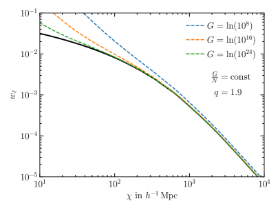
In Fig. 20 we show the $w_{\ell=\ell^{\prime}=42}(\chi,\chi)$ with three different values of $G$, the size of the integration interval. For the same biasing parameter $q=1.9$. With width $G=\ln(10^{8})$ that we adopted when calculating $\xi_{\ell}^{\nu}(r)$, the aliasing effect is clearly visible on all $\chi$ values that we show here. The aliasing effect does get milder as we increase the interval $G$. In order to get a reliable result for $\chi>${10}^{2}\text{\,}{\mathrm{\text{$h$}}}^{-1}\text{\,}\mathrm{Mpc}$$, however, we need to choose the interval over 24 orders of magnitude in $k$ space.

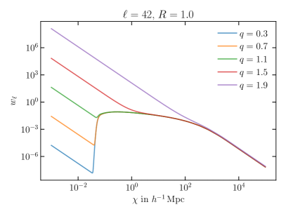
We find that biasing the convolved integrand provides a more efficient way of reducing the aliasing effect. That is, when adopting a smaller $q$ value, the integrand decays fast enough to suppress the aliasing effect. For example, we show the $w_{\ell=\ell^{\prime}=42}(\chi,\chi)$ for five values of $q$ between $0.3$ and $1.9$ in the left panel of Fig. 21. It turns out that one must take $q\lesssim 1.5$ in order to suppress the aliasing effect on cosmologically relevant scales $\chi\gtrsim$100\text{\,}{\mathrm{\text{$h$}}}^{-1}\text{\,}\mathrm{Mpc}$$. On the other hand, the right panel of Fig. 21 shows that all values of $q$ yield an accurate calculation of $w_{\ell=\ell^{\prime}=42}(\chi,\chi)$ on all cosmologically relevant scales $\chi\gtrsim$100\text{\,}{\mathrm{\text{$h$}}}^{-1}\text{\,}\mathrm{Mpc}$$. Finally, Fig. 22 shows the same for $\ell=1000$, and $R=1,0.99$. Here, too, $q\lesssim 1.1$ results in a small error at $\chi>$100\text{\,}{\mathrm{\text{$h$}}}^{-1}\text{\,}\mathrm{Mpc}$$.

Appendix C Transformation matrix from 2-FAST and trapezoidal method

Figure 23: Top panels: Same as Fig. 8, except using the traditional method Eq. (41). The graph is much more noisy than the 2-FAST method, due to undersampling of the oscillations of the Bessel functions, which is avoided by the 2-FAST method. Bottom panels: To facilitate comparison, we here show the difference between the 2-FAST algorithm Eq. (IV.2) and the traditional method. At small $k_{n}$, the differences are small, whereas at large $k_{n}$ the differences are the biggest.

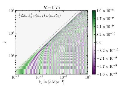
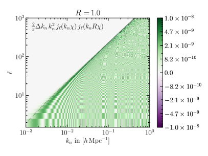
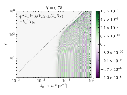
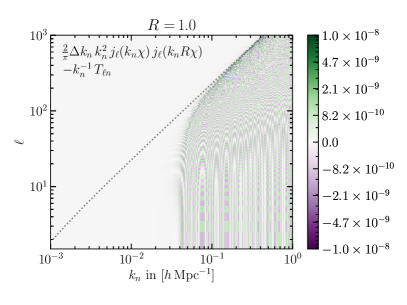
Fig. 23 shows the transformation matrix for the case of two spherical Bessel functions using the traditional method Eq. (41) (left) as well as the difference to the 2-FAST algorithm (right). The two matrices agree on large scales [$k\simeq\sqrt{\ell(\ell+1)}$], but show quite different behaviors on small scales (larger $k$). This is because the traditional trapezoidal method directly samples the multiplication of two spherical Bessel functions which are very oscillatory, while the 2-FAST transformation matrix effectively averages over these high-$k$ oscillations. An accurate integration, therefore, demands much denser sampling for the trapezoidal method than the 2-FAST method.

Appendix D Contiguous relations for the Gauss hypergeometric function

The Gauss hypergeometric function ${}_{2}F_{1}(a,b,c,z)$ is defined by the Gauss series:

$${}_{2}F_{1}(a,b,c,z) =\sum_{s=0}^{\infty}\frac{(a)_{s}(b)_{s}}{(c)_{s}}\,\frac{z^{s}}{s!}=1+\frac{ab}{c}\,z+\frac{a(a+1)\,b(b+1)}{c(c+1)}\,\frac{z^{2}}{2}+\cdots$$ (87)

where the Pochhammer symbol is defined as $(a)_{s}=a(a+1)\cdots(a+s-1)$. We find that the key to calculating the Gauss hypergeometric function is to exploit its contiguous relations:

$$(c-a)F(a-1,b,c,z)+(2a-c+(b-a)z)F(a,b,c,z)+a(z-1)F(a+1,b,c,z) =0$$ (88a)

$$(b-a)F(a,b,c,z)+aF(a+1,b,c,z)-bF(a,b+1,c,z) =0$$ (88b)

$$(c-a-b)F(a,b,c,z)+a(1-z)F(a+1,b,c,z)-(c-b)F(a,b-1,c,z) =0$$ (88c)

$$c(a+(b-c)z)F(a,b,c,z)-ac(1-z)F(a+1,b,c,z)+(c-a)(c-b)zF(a,b,c+1,z) =0$$ (88d)

$$(c-a-1)F(a,b,c,z)+aF(a+1,b,c,z)-(c-1)F(a,b,c-1,z) =0$$ (88e)

$$c(1-z)F(a,b,c,z)-cF(a-1,b,c,z)+(c-b)zF(a,b,c+1,z) =0$$ (88f)

$$(a-1+(b+1-c)z)F(a,b,c,z)+(c-a)F(a-1,b,c,z)-(c-1)(1-z)F(a,b,c-1,z) =0$$ (88g)

$$c(c-1)(z-1)F(a,b,c-1,z)+c(c-1-(2c-a-b-1)z)F(a,b,c,z)+(c-a)(c-b)zF(a,b,c+1,z) =0\,,$$ (88h)

that one can find, for example, in DLMF . Note that we can generate more relations by using the symmetry between $a$ and $b$

$${}_{2}F_{1}(a,b,c,z)={}_{2}F_{1}(b,a,c,z)$$ (89)

which follows from the series definition in Eq. (87).

Appendix E Computing the Gauss hypergeometric function

Computing the Gauss hypergeometric function ${}_{2}F_{1}(a,b,c,z)$ with the parameters that we need in Eq. (31) is a challenge. In particular, the first parameter $a=\frac{1}{2}(-\ell+\ell^{\prime}+n)$ typically contains a large imaginary component, for which case we cannot apply the general methods of calculating ${}_{2}F_{1}$ in the literature (Michel and Stoitsov, 2008; Johansson, 2016). The method we present here fills this gap for the special case that we face in computing Eq. (31). We accomplish this by using analytical solutions when $\ell=0$ and recurrence relations that we construct from the hypergeometric function’s contiguous relations Eqs. (88a)–(88h).

In this section, we focus on the recurrence relation along $\ell\rightarrow\ell+1$ (thick black arrows in Fig. 6). The recurrence relations along $\Delta\ell\rightarrow\Delta\ell\pm 2$ are needed for a few iterations only, and so they are not as critical. Hence, we only consider $\Delta\ell=\mathrm{const}$ here. We shall present the details of the full calculation of $M_{\ell\ell^{\prime}}^{q}$ for general cases with $\Delta\ell=\ell^{\prime}-\ell\neq\mathrm{const}$ in App. F. In this section we only consider $\Delta\ell=4$ when a specific $\Delta\ell$ is needed.

Furthermore, for simplicity, we only treat the hypergeometric function ${}_{2}F_{1}$, without the $\ell$-dependent prefactors in Eqs. (30)–(31). Nevertheless, the method presented in this section is the core of evaluating $M_{\ell\ell^{\prime}}^{q}$ because the prefactor merely scales the recurrence relations, without changing the stability properties.

Comparing with Eq. (31), we identify $a$, $b$, $c$, and $z$ as

$$a=\, \frac{1}{2}n+\frac{1}{2}\Delta\ell=\frac{1}{2}\left(q-1-it+\Delta\ell\right)$$ (90)

$$b=\, \ell+\frac{1}{2}+\frac{1}{2}n+\frac{1}{2}\Delta\ell=c+a-1-\Delta\ell$$ (91)

$$c=\, \ell+\frac{3}{2}+\Delta\ell$$ (92)

$$z=\, R^{2}\,,$$ (93)

and we introduce a shorthand notation

$$F_{\ell}[i,j,k] ={}_{2}F_{1}(a+i,b+j,c+k,z)$$ (94)

to avoid clutter.

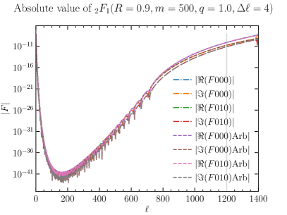
Finally, in order to test the accuracy of our results, we have checked out several software implementations of the Gauss hypergeometric function. One of the best we have found is the Arb library (Johansson, 2017). Arb is an arbitrary precision floating point library with automatic rigorous error bounds. Bindings for the Julia language exist in the package Nemo.

E.1 Recurrence relation for the $\ell$-ladder

We have calculated ${}_{2}F_{1}$ based on the recurrence relation that relates $F_{\ell}[0,0,0]={}_{2}F_{1}(a,b,c;z)$ to $F_{\ell+1}[0,0,0]={}_{2}F_{1}(a,b+1,c+1;z)=F_{\ell}[0,1,1]$. The key is to exploit the contiguous relations of the Gauss hypergeometric functions given in App. D. Among many possible relations, we choose a recurrence relation using $F_{\ell}[0,0,0]$ and $F_{\ell}[0,1,0]$. That is, we use

Eq. (88f) with $(a,b,c)\rightarrow$	$(b+1,a,c)$
Eq. (88e) with $(a,b,c)\rightarrow$	$(b+1,a,c+1)$

to find

$$(c-a)zF_{\ell}[0,1,1] =cF_{\ell}[0,0,0]-c(1-z)F_{\ell}[0,1,0]$$ (95)

$$(b+1)F_{\ell}[0,2,1] =-(c-b-1)F_{\ell}[0,1,1]+cF_{\ell}[0,1,0]\,.$$ (96)

This way we can compute $F_{\ell+1}[0,0,0]=F_{\ell}[0,1,1]$ and $F_{\ell+1}[0,1,0]=F_{\ell}[0,2,1]$ from $F_{\ell}[0,0,0]$ and $F_{\ell}[0,1,0]$.

We then combine the recurrence relations Eqs. (95)–(96) with analytical solutions at $\ell=0$. We define the function

$$g^{\pm}(n,R) =(1+R)^{n}\pm(1-R)^{n}$$ (97)

Then, for $\Delta\ell=4$ this gives the following analytical solution:

$$F_{0,4}[0,0,0] =\frac{945}{2m\big{(}576-820m^{2}+273m^{4}-30m^{6}+m^{8}\big{)}R^{9}}$$

$$\quad\times\bigg{[}-5mR\big{[}21+(-11+2m^{2})R^{2}\big{]}\,g^{+}(m,R)$$

$$\qquad\quad+\big{[}105+45(-2+m^{2})R^{2}+(9-10m^{2}+m^{4})R^{4}\big{]}\,g^{-}(m,R)\bigg{]}$$ (98)

$$F_{0,4}[0,1,0] =\frac{945}{2(-5+n)(-3+n)(-2+n)(-1+n)n(1+n)(2+n)(3+n)(5+n)R^{9}}$$

$$\quad\times\bigg{[}\big{[}105+15(-5+3n^{2})R^{2}+n^{2}(-4+n^{2})R^{4}\big{]}\,g^{-}(-n,-R)$$

$$\qquad\quad-nR\,\big{[}105+(-4+n^{2})R^{2}(10+R^{2})\big{]}\,g^{+}(-n,-R)\bigg{]}$$ (99)

where $m=1-n$. These expressions are numerically unstable for $R\sim 0$. For simplicity one may use 256-bit arbitrary precision floating point arithmetic to evaluate these. Since these expressions are cosmology independent and only need to be evaluated once, the performance is not very critical here.

It turns out that, however, unless $z=R^{2}\simeq 1$, the forward-directional recurrence relation Eqs. (95)–(96) are unstable under an injection of small noise (which happens, for example, due to the numerical round-off error at each recursion step).

Instead, we find that the reverse, backward-directional recurrence relation,

$$F_{\ell}[0,1,0] =c^{-1}(c-b-1)F_{\ell}[0,1,1]+c^{-1}(b+1)F_{\ell}[0,2,1]$$ (100)

$$F_{\ell}[0,0,0] =c^{-1}(c-a)zF_{\ell}[0,1,1]+(1-z)F_{\ell}[0,1,0],$$ (101)

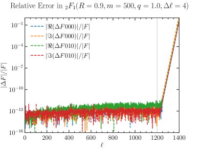
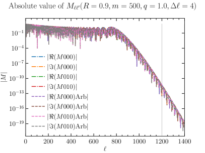
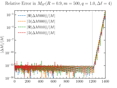
is quite stable so that the noise decays while the recursion proceeds along the backward direction of $\ell\to\ell-1$. This is the basis of Miller’s algorithm Bickley et al. (1952) that we have implemented here. Fig. 24 shows the performance and error propagation for the backward recursion.

On the other hand, for the backward recursion, we do not have the luxury of an analytical expression for the initial condition at large $\ell$ values. The challenge now is, therefore, to find suitable values to start the recursion with. Again, the key fact is that the backward recursion is so stable that any deviation from the true value (noise) decays quickly. The general strategy we adopt, therefore, is to start the recursion from some large $\ell_{\mathrm{seed}}$, which is sufficiently larger than the maximum multipole $\ell_{\mathrm{max}}$ that we want to calculate the $F_{\ell}[0,0,0]$ for. Specifically, we increase $\ell_{\text{seed}}$ until convergence is reached for the resulting $F_{\ell_{\mathrm{max}}}[0,0,0]$ and $F_{\ell_{\mathrm{max}}}[0,1,0]$ within $10^{-10}$ accuracy. That is, we require

$$\frac{||\vec{F}_{\ell_{\mathrm{max}}}^{(\mathrm{new}~{}\ell_{\mathrm{seed}})}-\vec{F}_{\ell_{\mathrm{max}}}^{(\mathrm{old}~{}\ell_{\mathrm{seed}})}||}{||\vec{F}_{\ell_{\mathrm{max}}}^{(\mathrm{new}~{}\ell_{\mathrm{seed}})}||} <${10}^{-10}$$$ (102)

where we define $\vec{F}_{\ell}=(F_{\ell}[0,0,0],F_{\ell}[0,1,0])$, and we define the norm as the Euclidean distance: $||\vec{x}||\equiv\sqrt{\Re(x_{1})^{2}+\Im(x_{1})^{2}+\Re(x_{2})^{2}+\Im(x_{2})^{2}}$, with $x_{1}=F[0,0,0]$ and $x_{2}=F[0,1,0]$, and $\Im(z)$ is the imaginary part of $z$.

In principle, any initial guess for $F_{\ell_{\mathrm{seed}}}[0,0,0]$ should work. When choosing a value close to the true value, however, the recursion chain converges to the true $F_{\ell}[0,0,0]$ value much faster. In the remainder of this section, we shall present our implementation of setting up the initial conditions.

Figure 24: Demonstration of Miller’s algorithm. Top Left: The absolute value of the real and imaginary parts of the hypergeometric function calculated via recurrence relations is compared with the arbitrary precision library Arb(Johansson, 2017). Top Right: The relative difference between the recurrence relation method and Arb is shown. As shown, large errors die out before our target $\ell_{\mathrm{max}}=1200$ indicated by the gray vertical line is reached. Bottom Panels: Same as the top two panels, but for $M^{q}_{\ell\ell^{\prime}}$ instead of ${}_{2}F_{1}$.

E.2 Setting up the initial condition for the backward recursion for $z\ll 1$

Here we show the method by which we set up the initial condition at some large $\ell_{\mathrm{seed}}$ for the $z=R^{2}\ll 1$ case, exploiting that the error in the initial values will die out when stepping down the $\ell$ ladder. First, we define

$$\vec{F}_{\ell} =\left(\begin{matrix}F_{\ell}[0,0,0]\\ F_{\ell}[0,1,0]\end{matrix}\right)\,,$$ (103)

so that we can represent the recursion relation in matrix form $\vec{F}_{\ell+1}=A_{\ell}\cdot\vec{F}_{\ell}$ with

$$A_{\ell} =\left(\begin{matrix}\frac{c}{c-a}\,\frac{1}{z}&-\frac{c}{c-a}\,\frac{1-z}{z}\\ \frac{c}{c-a}\,\frac{a-\Delta\ell}{c+a-\Delta\ell}\,\frac{1}{z}&\frac{c}{c+a-\Delta\ell}\big{[}1+\frac{\Delta\ell}{c-a}\,\frac{1-z}{z}\big{]}\end{matrix}\right)$$ (104)

which follows from Eqs. (95)–(96), and we used $b=c+a-1-\Delta\ell$. The inverse transformation is then given as

$$A_{\ell}^{-1} =\left(\begin{matrix}z-\frac{a}{c}+\frac{\Delta\ell}{c}\,(1-z)&\left[1+\frac{a}{c}-\frac{\Delta\ell}{c}\right](1-z)\\ -\frac{a}{c}+\frac{\Delta\ell}{c}&1+\frac{a}{c}-\frac{\Delta\ell}{c}\end{matrix}\right)\,.$$ (105)

Applying the recursion multiple times, we can relate $\vec{F}_{\ell}$ to $\vec{F}_{\ell+m}$ as

$$\vec{F}_{\ell+m} =A_{\ell}^{[m]}\vec{F}_{\ell}$$ (106)

$$\vec{F}_{\ell} =A_{\ell}^{[-m]}\vec{F}_{\ell+m}\,,$$ (107)

where we introduce the notation for the matrix

$$A_{\ell}^{[m]} =A_{\ell+m-1}\cdots A_{\ell}$$ (108)

$$A_{\ell}^{[-m]} =A_{\ell}^{-1}\cdots A_{\ell+m-1}^{-1}\,.$$ (109)

Note that $A_{\ell}^{[-m]}\,A_{\ell}^{[m]}=1$. The matrix $A_{\ell}^{[m]}$ raises the $\ell$ to $\ell+m$, whereas the matrix $A_{\ell}^{[-m]}$ lowers $\ell+m$ down to $\ell$.

Just to show the point directly, let us analyze the stability properties in the $\ell\rightarrow\infty$ limit, where the lowering matrix becomes

$$A_{\infty}^{-1} =\left(\begin{matrix}z&1-z\\ 0&1\end{matrix}\right),$$ (110)

whose eigenvalues are $\lambda_{1}=1$ and $\lambda_{2}=z$, with eigenvectors $\vec{x}_{1}=1/\sqrt{2}(1,1)$ and $\vec{x}_{2}=(1,0)$. That is, the $\vec{x}_{2}$ component of the solution will be suppressed by a factor $z^{n}$ when lowering $\ell$ by $n$ steps, whereas the $x_{1}$ component is the dominant solution in the backwards direction. This motivates us to define the initial value of the recursion at $\ell_{\mathrm{seed}}$ as

$$\vec{F}_{\ell_{\text{seed}}}=\frac{\lambda}{\sqrt{2}}\left(\begin{matrix}1\\ 1\end{matrix}\right)$$ (111)

with a complex constant $\lambda$ that we fix so that $\vec{F}_{0}^{\text{seeded}}=A_{0}^{[-\ell_{\text{seed}}]}\vec{F}_{\ell_{\text{seed}}}$ matches the analytical solution Eqs. (E.1)–(99).

E.3 Extension to general $z$

The method we have described in App. E.2 works best for small $z$ because the error in the initial condition decays as $z^{n}$. For the $z=R^{2}\sim 1$ cases, therefore, the error in the initial condition decays slowly so that one needs to set $\ell_{\mathrm{seed}}$ much larger than $\ell_{\mathrm{max}}$. In the extreme case of $z=1$, the initial error does not die at all. In this section, we summarize our method of generating the initial condition at $\ell_{\mathrm{seed}}$ for these cases.

For the $z\sim 1$ cases, we use the fact that the forward recursion is more stable than the $z<1$ cases. For that, we first attempt to invert the matrix $A_{0}^{[-\ell_{\text{seed}}]}$ to find the matrix for the forward recursion. Because the matrices $A_{\ell}^{-1}$ are invertible, in principle, the final matrix $A_{0}^{[-\ell_{\text{seed}}]}$ must be invertible as well. If the forward recursion is stable enough that $A_{0}^{[-\ell_{\text{seed}}]}$ is numerically invertible, we find $\vec{F}_{\ell_{\mathrm{seed}}}$ from $\vec{F}_{0}$ and the matrix $A_{0}^{[\ell_{\text{seed}}]}$ for the forward recursion; we then run the backward recursion in order to clean any possible error caused by numerical round-off. Often there are cases, however, where, as a result of accumulated numerical round-off error at each step of the matrix multiplication, the resulting $A_{0}^{[-\ell_{\text{seed}}]}$ ends up singular (noninvertible) or, for the same reason, numerical infinities appear in the inverted matrix. In that case, we use the seeding value in Eq. (111), and then we choose $\lambda\in\mathbb{C}$ such that we match the analytical solution Eqs. (E.1)–(99) at $\ell=0$:

$$\vec{F}_{0} =A_{0}^{[-\ell_{\text{seed}}]}\,\frac{\lambda}{\sqrt{2}}\left(\begin{matrix}1\\ 1\end{matrix}\right)\,.$$ (112)

Whether the inversion of the matrix is successful ($R\sim 1$ cases) or not ($R\ll 1$ cases), any error introduced by numerical round-off will be corrected both by the choice of $\lambda$ and by running the backward recursion from $\ell_{\text{seed}}$ down to $\ell_{\mathrm{max}}$. Hence, this approach works for all values of $z$.

E.3.1 Special cases

The special cases $m=0$ (the direct current (DC) mode), $z=R^{2}=1$, and $z=R^{2}=0$ need to be handled separately.

• The DC mode: With the above approach, we may run into division-by-zero problems when the mode $m=0$. Then for some choice of $q$ and $\Delta\ell$ it may happen that $n+\Delta\ell=0$, which implies $a=0$. In this case, however, we have the trivial solution

  $$F_{\ell}[0,0,0] =1$$ (113)

  $$F_{\ell}[0,1,0] =1$$ (114)

  for any $\ell$. This follows from Eq. (87).

• $z=1$: For the case $R^{2}=1$, we can speed up the computation by using the analytical expression for the initial condition at any $\ell$

  $$F_{\ell}[0,0,0] =\frac{\Gamma(c)\,\Gamma(c-a-b)}{\Gamma(c-a)\,\Gamma(c-b)}\,.$$ (115)

  For $F_{\ell}[0,1,0]$ Eq. (115) does not give a finite answer when $q=1$ and $t=0$. Hence, it is best to require $q\neq 1$.

• $z=0$: For the case $R=0$, the $w_{\ell\ell^{\prime}}(\chi,\chi^{\prime})=0$ for all $\ell^{\prime}>0$ due to the vanishing of the spherical Bessel function at the origin. Thus no calculation is required.

E.4 Underflow protection

The hypergeometric function values (and $M^{q}_{\ell\ell^{\prime}}$ as well) may under some circumstances (especially when the number of sample points $N$ of the power spectrum is large, e.g. $R=0.99$, $q=0.5$, $m=4100$, $G=23.6$, $\ell_{\mathrm{max}}=1200$) suffer from underflow error when represented as a double precision number. That is, starting at $\ell=0$, which can generally be represented in doubles, $|{}_{2}F_{1}|$ gets smaller and smaller going towards higher $\ell$, and it eventually hits the underflow value for double precision numbers $|{}_{2}F_{1}|<${10}^{-308}$$.

We must, therefore, take care of the case where the seeding value becomes $\vec{F}_{\ell_{\text{seed}}}=0$ as a result of the underflow. We detect this when one or more of the elements in $A_{0}^{[-\ell_{\text{seed}}]}$ becomes $\pm{}\infty$ as represented by double precision. The solution we adopt here is to store the largest $\ell_{\text{finite}}<\ell_{\mathrm{max}}$ where no underflow occurs, and approximate ${}_{2}F_{1}\approx 0$ for $\ell>\ell_{\text{finite}}$.

Appendix F Recursion for the full kernel

In this appendix we derive the recurrence relations that are valid not just for the hypergeometric function, but for the full kernel $M^{q}_{\ell\ell^{\prime}}(t,R)$ in Eq. (30). We also detail the recursions to move towards any even $\Delta\ell\equiv\ell^{\prime}-\ell$ (thick gray arrows in Fig. 6), for the two cases $R\leq 1$ and $R>1$. These two cases need to be treated separately due to Eq. (34). Note, however, that due to the symmetry $w_{\ell\ell^{\prime}}(\chi,\chi^{\prime})=w_{\ell^{\prime}\ell}(\chi^{\prime},\chi)$, only one of the two cases is actually needed, although for some computations (e.g. lensing-galaxy cross-correlation, see Sec. V.3) it is convenient to be able to compute both cases explicitly.

As in Eqs. (90)–(93) $a$, $b$, $c$, and $z$ will be the parameters to the hypergeometric function ${}_{2}F_{1}(a,b;c;z)$ in Eq. (31).

To get the full kernel $M^{q}_{\ell\ell^{\prime}}(t,R)$, the hypergeometric function needs to be multiplied by the prefactors in Eqs. (30)–(31). The prefactor is

$$A_{\ell,\Delta\ell} =(k_{0}\chi_{0})^{it-q}\,2^{n-2}\,\pi\,R^{\ell+\Delta\ell}\,\frac{\Gamma\big{[}\ell+\frac{1}{2}+\frac{1}{2}n+\frac{1}{2}\Delta\ell\big{]}}{\Gamma\big{[}1-\frac{1}{2}n-\frac{1}{2}\Delta\ell\big{]}\,\Gamma\big{(}\ell+\frac{3}{2}+\Delta\ell\big{)}}$$ (116)

where $\Delta\ell=\ell^{\prime}-\ell$. We get

$$A_{\ell+1,\Delta\ell} =A_{\ell,\Delta\ell}\,R\,\frac{\ell+\frac{1}{2}+\frac{1}{2}n+\frac{1}{2}\Delta\ell}{\ell+\frac{3}{2}+\Delta\ell}=A_{\ell,\Delta\ell}\,\frac{bR}{c}$$ (117)

which adds another factor to our recursion relations Eqs. (100)–(101). Since this multiplies all elements in the recursion matrix by the same number, the ratio of the eigenvalues is the same as without the prefactor, and hence this does not change the stability properties of the relation discussed in App. E.

Our recursion relations along $\ell\rightarrow\ell+1$ are stable in the backward direction for any $\Delta\ell=0,\pm 2,\pm 4$ (which are all we have tested). The recursion relations detailed below to change $\Delta\ell$ are stable in the $\Delta\ell\rightarrow\Delta\ell-2$ direction for $R<1$, and they are stable in the $\Delta\ell\rightarrow\Delta\ell+2$ direction for $R>1$. Thus, we perform the $\Delta\ell=\mathrm{const}$ recursions with $\Delta\ell=4$ for $R<1$, and with $\Delta\ell=-4$ for $R>1$. Note, however, that due to the symmetry Eq. (34), the initialization with $\Delta\ell=4$ as described in App. E is also valid for the $R>1$ case.

The relations to move towards $\Delta\ell\neq 0$ are determined by Eqs. (90)–(93). Our recursion relations along $\ell\rightarrow\ell-1$ give us $F_{\ell}[0,1,0]$ along with $F_{\ell}[0,0,0]$ (or their $M^{q}_{\ell\ell}$ equivalent). However, in the sections below we derive the recursions using the values $F[0,0,0]$ and $F[0,-1,0]$. To go from $F[0,1,0]$ we use Eq. (88a) with $a\leftrightarrow b$ to get

$$(c-b)F[0,-1,0] =b(1-z)F[0,1,0]-\big{(}2b-c+(a-b)z\big{)}F[0,0,0]$$ (118)

In this section we will generally drop the subscript $\ell$, and sometimes use $\Delta\ell=\ell-\ell^{\prime}$ as a subscript instead. $a$, $b$, and $c$, which are functions of $\ell$ and $\Delta\ell$, are understood to take on their values at $F[0,0,0]$ in any given equation. In the remainder of this appendix, we derive the $\Delta\ell\neq 0$ relations.

F.1 Towards $\Delta\ell=-2$ when $R<1$

To calculate $\Delta\ell=-2$ we need $F[-1,-1,-2]$. We start with Eq. (88e) with $(a,b,c)\rightarrow(a-1,b-1,c-1)$ to get

$$F[-1,-1,-2] =\frac{c-1-a}{c-2}\,F[-1,-1,-1]+\frac{a-1}{c-2}\,F[0,-1,-1]$$ (119)

Eq. (88f) with $(a,b,c)\rightarrow(a,b-1,c-1)$ gives

$$F[-1,-1,-1] =(1-z)\,F[0,-1,-1]+\frac{c-b}{c-1}\,z\,F[0,-1,0]$$ (120)

and Eq. (88e) with $a\leftrightarrow b$ and$(a,b,c)\rightarrow(a,b-1,c)$ gives

$$F[0,-1,-1] =\frac{c-b}{c-1}\,F[0,-1,0]+\frac{b-1}{c-1}\,F[0,0,0]$$ (121)

Putting the last three together, one at a time, we get

$$F[-1,-1,-2] =\frac{(c-1-a)(1-z)+a-1}{c-2}\,F[0,-1,-1]+\frac{c-1-a}{c-2}\,\frac{c-b}{c-1}\,z\,F[0,-1,0]$$ (122)

$$=\frac{c-b}{c-1}\,F[0,-1,0]+\frac{c-2-(c-1-a)z}{(c-2)(c-1)}\,(b-1)\,F[0,0,0]$$ (123)

From Eq. (116) we see that

$$A_{\ell,\Delta\ell-2} =A_{\ell,\Delta\ell}\,R^{-2}\,\frac{\big{(}\ell-\frac{1}{2}+\Delta\ell\big{)}\big{(}\ell+\frac{1}{2}+\Delta\ell\big{)}}{\big{(}\ell-\frac{1}{2}+\frac{1}{2}\Delta\ell+\frac{1}{2}n\big{)}\big{(}1-\frac{1}{2}\Delta\ell-\frac{1}{2}n\big{)}}$$ (124)

$$=A_{\ell,\Delta\ell}\,R^{-2}\,\frac{(c-2)(c-1)}{(b-1)(1-a)}$$ (125)

where $a$, $b$, and $c$ are evaluated at $\Delta\ell$. Hence, writing $\tilde{F}_{\Delta\ell}=A_{\ell,\Delta\ell}\,F$ we get

$$\tilde{F}_{-2}[-1,-1,-2] =\frac{(c-b)(c-2)}{(b-1)(1-a)R^{2}}\,\tilde{F}_{0}[0,-1,0]+\frac{c-2-(c-1-a)z}{(b-1)(1-a)R^{2}}\,(b-1)\,\tilde{F}_{0}[0,0,0]$$ (126)

$$\tilde{F}_{-2}[0,0,0] =\frac{(c-2)(c-1)}{(b-1)(1-a)R^{2}}\,\tilde{F}_{0}[0,0,0]$$ (127)

which keeps the factor $A_{\ell,\Delta\ell}$ the same for the two hypergeometric function values, and allows us to use these as the starting values for a recursion towards $\Delta\ell=-4$.

F.2 Towards $\Delta\ell=-4$ when $R<1$

We also need to go towards $\Delta\ell=-4$, or $F[-2,-2,-4]$. We do this by building a recursion from $F[0,0,0]$ and $F[-1,-1,-2]$. We use the following seven relations,

Eq. (88e) with $(a,b,c)\rightarrow$	$(b-1,a,c)$
Eq. (88h) with $(a,b,c)\rightarrow$	$(a,b-1,c-1)$
Eq. (88f) with $(a,b,c)\rightarrow$	$(a,b-1,c-2)$
Eq. (88c) with $(a,b,c)\rightarrow$	$(a-1,b-1,c-2)$
Eq. (88e) with $(a,b,c)\rightarrow$	$(b-2,a-1,c-2)$
Eq. (88h) with $(a,b,c)\rightarrow$	$(a-1,b-2,c-3)$
Eq. (88f) with $(a,b,c)\rightarrow$	$(a-1,b-2,c-4)$

which result in the following equations:

$$(c-1)F[0,-1,-1] =(c-b)F[0,-1,0]+(b-1)F[0,0,0]$$ (128)

$$(c-1)(c-2)(1-z)F[0,-1,-2] =(c-1)(c-2-(2c-2-b-a)z)F[0,-1,-1]$$

$$\quad+(c-b)(c-1-a)zF[0,-1,0]$$ (129)

$$(c-2)(1-z)F[0,-1,-2] =(c-2)F[-1,-1,-2]-(c-1-b)zF[0,-1,-1]$$ (130)

$$(c-1-b)F[-1,-2,-2] =(c-a-b)F[-1,-1,-2]+(a-1)(1-z)F[0,-1,-2]$$ (131)

$$(c-3)F[-1,-2,-3] =(c-b-1)F[-1,-2,-2]+(b-2)F[-1,-1,-2]$$ (132)

$$(c-3)(c-4)(1-z)F[-1,-2,-4] =(c-3)(c-4-(2c-4-a-b)z)F[-1,-2,-3]$$

$$\quad+(c-2-a)(c-1-b)zF[-1,-2,-2]$$ (133)

$$(c-4)F[-2,-2,-4] =(c-4)(1-z)F[-1,-2,-4]+(c-2-b)zF[-1,-2,-3]$$ (134)

The first three can be solved for $(1-z)F[0,-1,-2]$. Inserting the first into the second and third we get

$$(c-1)(c-2)(1-z)F[0,-1,-2] =(c-2-(c-1-b)z)(c-b)F[0,-1,0]$$

$$\quad+(c-2-(2c-2-b-a)z)(b-1)F[0,0,0]$$ (135)

$$(c-1)(c-2)(1-z)F[0,-1,-2] =(c-1)(c-2)F[-1,-1,-2]-(c-b)(c-1-b)zF[0,-1,0]$$

$$\quad-(c-1-b)z(b-1)F[0,0,0]$$ (136)

and then solving the second for $F[0,-1,0]$ and inserting into the third, we get

$$(1-z)F[0,-1,-2] =\frac{c-2-(c-1-b)z}{c-2}\,F[-1,-1,-2]-(c-1-a)z(c-1-b)z\frac{b-1}{(c-1)(c-2)^{2}}\,F[0,0,0]$$ (137)

To get $F[-2,-2,-4]$ we start with the last of Eqs. (128)–(134) and then continue using each upwards in succession. We get

$$F[-2,-2,-4] =\frac{c-4-(c-2-a)z}{c-4}\,F[-1,-2,-3]+\frac{(c-2-a)(c-1-b)z}{(c-3)(c-4)}\,F[-1,-2,-2]$$ (138)

$$=\frac{c-b-1}{c-3}F[-1,-2,-2]+\frac{(c-4-(c-2-a)z)(b-2)}{(c-3)(c-4)}\,F[-1,-1,-2]$$ (139)

$$=\frac{(c-a-2)(c-4-(b-2)z)}{(c-3)(c-4)}\,F[-1,-1,-2]+\frac{(a-1)(1-z)}{c-3}\,F[0,-1,-2]$$ (140)

$$=\frac{(c-a-2)(c-4-(b-2)z)(c-2)+(c-2-(c-1-b)z)(a-1)(c-4)}{(c-2)(c-3)(c-4)}\,F[-1,-1,-2]$$

$$\quad-(c-1-a)z(c-1-b)z\frac{(a-1)(b-1)}{(c-1)(c-2)^{2}(c-3)}\,F[0,0,0]$$ (141)

$$=\frac{(c-2)(c-4)-\big{[}a(c-b)+b(c-a)-3c+4\big{]}z}{(c-2)(c-4)}\,F[-1,-1,-2]$$

$$\quad-(c-1-a)z(c-1-b)z\frac{(a-1)(b-1)}{(c-1)(c-2)^{2}(c-3)}\,F[0,0,0]$$ (142)

The factor $A_{\ell,\Delta\ell}$ can be adjusted according to Eq. (125), where now $a$, $b$, and $c$ are evaluated at $\Delta\ell=-2$.

F.3 Towards $\Delta\ell=2$ when $R<1$

We need $F[1,1,2]$ in terms of $F[0,0,0]$ and $F[0,-1,0]$. To get $F[1,1,2]$ we use Eq. (88b) with $(a,b,c)\rightarrow(a,b+1,c+2)$ to reduce $a$, that is,

$$F[1,1,2] =\frac{b+1}{a}\,F[0,2,2]-\frac{b-a+1}{a}\,F[0,1,2]$$ (143)

We get $F[0,2,2]$ from Eq. (88e) with $a\leftrightarrow b$ and $(a,b,c)\rightarrow(a,b+1,c+2)$:

$$F[0,2,2] =\frac{c+1}{b+1}\,F[0,1,1]-\frac{c-b}{b+1}\,F[0,1,2]$$ (144)

$F[0,1,1]$ and $F[0,1,2]$ we can get from

Eq. (88e) with $(a,b,c)\rightarrow$	$(b,a,c+1)$
Eq. (88f) with $(a,b,c)\rightarrow$	$(b,a,c)$

which are

$$F[0,1,1] =-\frac{1}{b}\Big{[}(c-b)F[0,0,1]-cF[0,0,0]\Big{]}$$ (145)

$$F[0,0,1] =-\frac{c}{(c-a)z}\Big{[}(1-z)F[0,0,0]-F[0,-1,0]\Big{]}$$ (146)

By applying Eqs. (145)–(146) multiple times we get

$$F[1,1,2] =\frac{c+1}{a}\,F[0,1,1]-\frac{c+1-a}{a}\,F[0,1,2]$$ (147)

$$=\frac{c+1}{a}\,\frac{1}{z}\bigg{[}F[0,1,1]-F[0,0,1]\bigg{]}$$ (148)

$$=\frac{c+1}{a}\,\frac{c}{b}\,\frac{1}{z}\bigg{[}F[0,0,0]-F[0,0,1]\bigg{]}$$ (149)

$$=\frac{c+1}{a(c-a)}\,\frac{c}{b}\,\frac{1}{z^{2}}\bigg{[}(c-az)F[0,0,0]-cF[0,-1,0]\bigg{]}$$ (150)

where $a$, $b$, and $c$ are evaluated with the $\Delta\ell$ that corresponds to $F[0,0,0]$. For the full recursion we need to see how Eq. (116) changes. It is

$$A_{\ell,\Delta\ell+2} =A_{\ell,\Delta\ell}\,R^{2}\,\frac{\big{(}\ell+\frac{1}{2}+\frac{1}{2}\Delta\ell+\frac{1}{2}n\big{)}\big{(}-\frac{1}{2}\Delta\ell-\frac{1}{2}n\big{)}}{\big{(}\ell+\frac{3}{2}+\Delta\ell+1\big{)}\big{(}\ell+\frac{3}{2}+\Delta\ell\big{)}}$$ (151)

$$=-A_{\ell,\Delta\ell}\,R^{2}\,\frac{ab}{c(c+1)}$$ (152)

Combining with Eq. (150) we get

$$\tilde{F}[1,1,2] =\frac{1}{(c-a)z}\bigg{[}c\tilde{F}[0,-1,0]-(c-az)\tilde{F}[0,0,0]\bigg{]}$$ (153)

F.4 Towards $\Delta\ell=4$ when $R<1$

All we need here is to reverse the relations in Sec. F.2. That is, we are given $F[-2,-2,-4]$ and $F[-1,-1,-2]$, and we want to calculate $F[0,0,0]$. We can then shift the result to get the relation for $F[2,2,4]$ instead. Solving Eq. (142) for $F[0,0,0]$ we get

$$F[0,0,0] =\frac{(c-1)(c-2)(c-3)}{(a-1)(b-1)(c-4)(c-1-a)z(c-1-b)z}\bigg{[}$$

$$\qquad\Big{(}(c-2)(c-4)-\big{[}a(c-b)+b(c-a)-3c+4\big{]}z\Big{)}\,F[-1,-1,-2]$$

$$\qquad-(c-2)(c-4)F[-2,-2,-4]\bigg{]}$$ (154)

Applying the transformation $(a,b,c)\rightarrow(a+2,b+2,c+4)$ we get

$$F[2,2,4] =\frac{(c+3)(c+2)(c+1)}{(a+1)(b+1)c(c+1-a)z(c+1-b)z}\bigg{[}$$

$$\qquad\Big{(}(c+2)c-\big{[}(a+2)(c+2-b)+(b+2)(c+2-a)-3c-8\big{]}z\Big{)}\,F[1,1,2]$$

$$\qquad-(c+2)cF[0,0,0]\bigg{]}$$ (155)

F.5 Towards $\Delta\ell=-2$ when $R>1$

We use Eq. (34) to avoid arguments of the hypergeometric function $R^{2}>1$. That means that $\ell$ and $\ell^{\prime}$ get swapped, and we need to derive new recurrence relations. The swapping may be done by first writing $\Delta\ell$ in terms of $\ell$ and $\ell^{\prime}$, then swapping $\ell\leftrightarrow\ell^{\prime}$, and replacing $\ell^{\prime}=\ell+\Delta\ell$. Then we get

$$a =\tfrac{1}{2}n-\tfrac{1}{2}\Delta\ell$$ (156)

$$b =\ell+\tfrac{1}{2}+\tfrac{1}{2}n+\tfrac{1}{2}\Delta\ell=c+a-1+\Delta\ell$$ (157)

$$c =\ell+\tfrac{3}{2}$$ (158)

In other words,

$$(a,b,c) \rightarrow(a+1,b-1,c)\qquad\text{for }\Delta\ell=-2$$ (159)

$$(a,b,c) \rightarrow(a-1,b+1,c)\qquad\text{for }\Delta\ell=2\,.$$ (160)

Hence, we need $F[1,-1,0]$ and $F[-1,1,0]$ in terms of $F[0,0,0]$ and $F[0,-1,0]$.

For $\Delta\ell=-2$ we use Eq. (88b) with $b\rightarrow b-1$ to get

$$F[1,-1,0] =\frac{b-1}{a}\,F[0,0,0]-\frac{b-1-a}{a}\,F[0,-1,0]$$ (161)

To use Eq. (116) for the full kernel recursion in the case $R>1$, we need to exchange $\ell$ and $\ell^{\prime}$. Furthermore, Eq. (34) says that we need to let

$$\alpha \rightarrow R\alpha$$ (162)

$$R \rightarrow R^{-1}$$ (163)

Then,

$$A^{R>1}_{\ell,\Delta\ell} =\alpha^{it-q}\,2^{n-2}\,\pi\,R^{\ell}\,\frac{\Gamma\big{[}\ell+\frac{1}{2}+\frac{1}{2}\Delta\ell+\frac{1}{2}n\big{]}}{\Gamma\big{[}1+\frac{1}{2}\Delta\ell-\frac{1}{2}n\big{]}\,\Gamma\big{(}\ell+\frac{3}{2}\big{)}}$$ (164)

Thus,

$$A^{R>1}_{\ell,\Delta\ell-2} =A^{R>1}_{\ell,\Delta\ell}\,\frac{\frac{1}{2}\Delta\ell-\frac{1}{2}n}{\ell-\frac{1}{2}+\frac{1}{2}\Delta\ell+\frac{1}{2}n}$$ (165)

$$=-\frac{a}{b-1}\,A^{R>1}_{\ell,\Delta\ell}$$ (166)

F.6 Towards $\Delta\ell=-4$ when $R>1$

For this recursion we need $F[2,-2,0]$ in terms of $F[0,0,0]$ and $F[1,-1,0]$. We use

Eq. (88b) with $(a,b,c)\rightarrow$	$(a,b-1,c)$
Eq. (88c) with $(a,b,c)\rightarrow$	$(a,b-1,c)$
Eq. (88c) with $(a,b,c)\rightarrow$	$(b-2,a+1,c)$
Eq. (88b) with $(a,b,c)\rightarrow$	$(a+1,b-2,c)$

which results in

$$(b-1-a)F[0,-1,0] =(b-1)F[0,0,0]-aF[1,-1,0]$$ (167)

$$(c-b+1)F[0,-2,0] =(c-a-b+1)F[0,-1,0]+a(1-z)F[1,-1,0]$$ (168)

$$(c-b+1-a)F[1,-2,0] =(c-a-1)F[0,-2,0]-(b-2)(1-z)F[1,-1,0]$$ (169)

$$(a+1)F[2,-2,0] =(b-2)F[1,-1,0]-(b-a-3)F[1,-2,0]$$ (170)

F.7 Towards $\Delta\ell=2$ when $R>1$

We want $F[-1,1,0]$ from $F[0,0,0]$ and $F[0,-1,0]$. We use

Eq. (88a) with $(a,b,c)\rightarrow$	$(b,a,c)$
Eq. (88c) with $(a,b,c)\rightarrow$	$(b,a,c)$
Eq. (88c) with $(a,b,c)\rightarrow$	$(a-1,b+1,c)$

which results in

$$b(1-z)F[0,1,0] =(c-b)F[0,-1,0]+(2b-c+(a-b)z)F[0,0,0]$$ (171)

$$(c-a)F[-1,0,0] =(c-b-a)F[0,0,0]+b(1-z)F[0,1,0]$$ (172)

$$(c-a-b)F[-1,1,0] =(c-b-1)F[-1,0,0]-(a-1)(1-z)F[0,1,0]$$ (173)

From Eq. (164) we get

$$A^{R>1}_{\ell,\Delta\ell+2} =A^{R>1}_{\ell,\Delta\ell}\,\frac{\ell+\frac{1}{2}+\frac{1}{2}\Delta\ell+\frac{1}{2}n}{1+\frac{1}{2}\Delta\ell-\frac{1}{2}n}$$ (174)

$$=A^{R>1}_{\ell,\Delta\ell}\,\frac{b}{1-a}$$ (175)

F.8 Towards $\Delta\ell=4$ when $R>1$

For this recursion we need $F[-2,2,0]$ in terms of $F[0,0,0]$ and $F[-1,1,0]$. We use

Eq. (88b) with $(a,b,c)\rightarrow$	$(a-1,b,c)$
Eq. (88c) with $(a,b,c)\rightarrow$	$(b,a-1,c)$
Eq. (88c) with $(a,b,c)\rightarrow$	$(a-2,b+1,c)$
Eq. (88b) with $(a,b,c)\rightarrow$	$(a-2,b+1,c)$

which results in

$$(b-a+1)F[-1,0,0] =bF[-1,1,0]-(a-1)F[0,0,0]$$ (176)

$$(c-a+1)F[-2,0,0] =(c-a-b+1)F[-1,0,0]+b(1-z)F[-1,1,0]$$ (177)

$$(c-b-a+1)F[-2,1,0] =(c-b-1)F[-2,0,0]-(a-2)(1-z)F[-1,1,0]$$ (178)

$$(b+1)F[-2,2,0] =(b-a+3)F[-2,1,0]+(a-2)F[-1,1,0]$$ (179)

Appendix G Angular power spectrum with redshift-space distortion

To calculate redshift-space distortion (RSD) we use the well-known equation

$$C_{\ell} =\int\mathrm{d}{}z\,W(z)\,D(z)\int\mathrm{d}{}z^{\prime}\,W^{\prime}(z^{\prime})\,D(z^{\prime})\big{[}bb^{\prime}w_{\ell,00}-bf^{\prime}w_{\ell,02}-fb^{\prime}w_{\ell,20}+ff^{\prime}w_{\ell,22}\big{]}$$ (180)

where $W(z)$ and $W^{\prime}(z^{\prime})$ are window functions, $D(z)$ and $D(z^{\prime})$ are growth factors, $b$ and $b^{\prime}$ are linear biases, $f$ and $f^{\prime}$ dimensionless linear growth rates, and $w_{\ell,jj^{\prime}}(\chi,\chi^{\prime})$ were defined in Eq. (42). Using the recurrence relation for spherical Bessel-$j$ functions

$$j^{\prime}_{\ell}(x) =\frac{\ell}{2\ell+1}j_{\ell-1}(x)-\frac{\ell+1}{2\ell+1}j_{\ell+1}(x)$$ (181)

which results in

$$j^{\prime\prime}_{\ell}(x) =f_{-2}\,j_{\ell-2}(x)+f_{0}\,j_{\ell}(x)+f_{2}\,j_{\ell+2}(x)$$ (182)

where

$$f_{-2} =\frac{\ell(\ell-1)}{(2\ell-1)(2\ell+1)} f_{0} =-\frac{2\ell^{2}+2\ell-1}{(2\ell-1)(2\ell+3)} f_{2} =\frac{(\ell+1)(\ell+2)}{(2\ell+1)(2\ell+3)}\,.$$ (183)

We can express the terms in Eq. (180) in terms of $w_{\ell\ell^{\prime}}(\chi,\chi^{\prime})$ in the following way:

$$w_{\ell,00}(\chi,\chi^{\prime}) =w_{\ell,\ell}(\chi,\chi^{\prime})$$ (184)

$$w_{\ell,02}(\chi,\chi^{\prime}) =\left(\begin{matrix}f_{-2}&f_{0}&f_{2}\end{matrix}\right)\left(\begin{matrix}w_{\ell,\ell-2}(\chi,\chi^{\prime})\\ w_{\ell,\ell}(\chi,\chi^{\prime})\\ w_{\ell,\ell+2}(\chi,\chi^{\prime})\end{matrix}\right)$$ (185)

$$w_{\ell,20}(\chi,\chi^{\prime}) =\left(\begin{matrix}f_{-2}&f_{0}&f_{2}\end{matrix}\right)\left(\begin{matrix}w_{\ell-2,\ell}(\chi,\chi^{\prime})\\ w_{\ell,\ell}(\chi,\chi^{\prime})\\ w_{\ell+2,\ell}(\chi,\chi^{\prime})\end{matrix}\right)$$ (186)

$$w_{\ell,22}(\chi,\chi^{\prime}) =\left(\begin{matrix}f_{-2}&f_{0}&f_{2}\end{matrix}\right)\left(\begin{matrix}w_{\ell-2,\ell-2}&w_{\ell-2,\ell}&w_{\ell-2,\ell+2}\\ w_{\ell,\ell-2}&w_{\ell,\ell}&w_{\ell,\ell+2}\\ w_{\ell+2,\ell-2}&w_{\ell+2,\ell}&w_{\ell+2,\ell+2}\end{matrix}\right)\left(\begin{matrix}f_{-2}\\ f_{0}\\ f_{2}\end{matrix}\right)$$ (187)

where the $w_{\ell\ell^{\prime}}(\chi,\chi^{\prime})$ are given by Eq. (2).

Finally, note that

$$w_{\ell=i+j,\ell^{\prime}=i+k} =w_{\ell=i+j,\Delta\ell=k-j}$$ (188)

for any integers $i,j,k$. This means that we can calculate all $w_{\ell\pm 2,\ell\pm 2}(\chi,\chi^{\prime})$ from $w_{\ell,\ell\pm(0,2,4)}(\chi,\chi^{\prime})$ with $\ell\pm 2$, as indicated in Fig. 6 by the gray squares.

Appendix H The Lucas 1995 algorithm

As a benchmark calculation of the integrals over two Bessel functions, we use the algorithm proposed by Lucas (1995). We use it because it takes into account the entire integration range from $k=0$ to $k=\infty$ to high accuracy. Here, we summarize the algorithm applied to two spherical Bessel functions.

The idea of Lucas (1995) is to add and subtract a product of Bessel-$Y$ functions such that the product of Bessel-$J$ functions splits into two summands, each of which is asymptotically proportional to a sine function. That is,

$$j_{\ell}(k\chi)\,j_{\ell^{\prime}}(k\chi^{\prime}) =h_{1}(k;\ell,\ell^{\prime},\chi,\chi^{\prime})+h_{2}(k;\ell,\ell^{\prime},\chi,\chi^{\prime})$$ (189)

where

$$h_{1}(k;\ell,\ell^{\prime},\chi,\chi^{\prime}) =\tfrac{1}{2}\big{[}j_{\ell}(k\chi)\,j_{\ell^{\prime}}(k\chi^{\prime})-y_{\ell}(k\chi)\,y_{\ell^{\prime}}(k\chi^{\prime})\big{]}$$ (190)

$$h_{2}(k;\ell,\ell^{\prime},\chi,\chi^{\prime}) =\tfrac{1}{2}\big{[}j_{\ell}(k\chi)\,j_{\ell^{\prime}}(k\chi^{\prime})+y_{\ell}(k\chi)\,y_{\ell^{\prime}}(k\chi^{\prime})\big{]}\,.$$ (191)

The functions $h_{1}$ and $h_{2}$ behave asymptotically like sine functions. That is, for $k\gg 1$

$$h_{1}(k;\ell,\ell^{\prime},\chi,\chi^{\prime}) \sim\frac{1}{2\chi\chi^{\prime}k^{2}}\,\cos\big{[}(\chi+\chi^{\prime})k-\tfrac{\pi}{2}(\ell+\ell^{\prime}+1)\big{]}$$ (192)

$$h_{2}(k;\ell,\ell^{\prime},\chi,\chi^{\prime}) \sim\frac{1}{2\chi\chi^{\prime}k^{2}}\,\cos\big{[}(\chi-\chi^{\prime})k+\tfrac{\pi}{2}(\ell-\ell^{\prime})\big{]}\,.$$ (193)

Then for large $k$, the $h_{1}$ and $h_{2}$ terms are integrated between successive zeros, and the resulting alternating series is summed via a series acceleration. The series acceleration effectively integrates to $k=\infty$. We use the Levin u-transform as described in Press et al. (2007), which is also our algorithm of choice in Sec. III.2. We use the same quadosc algorithm as summarized there.

The case $\chi=\chi^{\prime}$ makes the function $h_{2}$ nonoscillatory for large $k$. This case is thus treated specially, by integrating the $h_{2}$ term to infinity via Gauss-Kronrod integration, and applying the quadosc algorithm to the $h_{1}$ term only.

For the evaluation of the spherical Bessel-$j$ and spherical Bessel-$y$ functions we use the Bessel function implementations included in the Julia programming language version 0.5.

For small $k$, the spherical Bessel-$y$ functions tend towards infinity, which can lead to catastrophic cancellation in the summation of the series. Hence, for the first few zeros, the integral is calculated directly via adaptive Gauss-Kronrod integration without the splitting into $h_{1}$ and $h_{2}$. We found that doing this for the first $\ell^{2}$ approximate zeros works fairly well, although for large $\ell$ that puts the burden of the calculation on the Gauss-Kronrod integration.

This procedure works well when $\ell$ is small. For large $\ell\gtrsim 200$ the adaptive Gauss-Kronrod integration needs to integrate over many oscillations, making the integration slow and possibly fail. Further investigation may reveal the exact nature of the problem. However, we find that reducing the relative error tolerance to ${10}^{-10}$ seems to work very well, and it is our choice in this paper.

Appendix I Generalized Limber approximation

In order to be applicable to the lensing-convergence-galaxy cross-correlation Eq. (58), we must extend the Limber approximation as written in Sec. V.2.1 to the cases $\ell\neq\ell^{\prime}$.

From the result of Ref. (Loverde and Afshordi, 2008),

$$\int_{0}^{\infty}dr\,f(r)\,J_{\nu}(kr) =k^{-1}\,f\!\left(\tfrac{\nu}{k}\right)+\mathcal{O}\big{(}f^{\prime\prime}\!\left(\tfrac{\nu}{k}\right)\big{)}\,,$$ (194)

where $\nu=\ell+\tfrac{1}{2}$ and $J_{\nu}(kr)$ are Bessel functions. Defining $c^{\prime}_{1}=b^{\prime}_{g}$ and $c^{\prime}_{2}=f^{\prime}$, and

$$A =\tfrac{3}{2}\Omega_{m}H_{0}^{2}\,\ell(\ell+1)$$ (195)

$$\varphi_{i}(\chi,\chi^{\prime}) =\frac{1}{\chi}\,\frac{\chi_{\star}-\chi}{\chi_{\star}}\,(1+z)\,D(z)D(z^{\prime})\,c_{i}^{\prime}\,\frac{1}{\sqrt{\chi\chi^{\prime}}}$$ (196)

$$j_{\ell}(k\chi) =\sqrt{\frac{\pi}{2k\chi}}\,J_{\ell+\frac{1}{2}}(k\chi)$$ (197)

$$\nu =\ell+\tfrac{1}{2}$$ (198)

$$\nu^{\prime} =\ell^{\prime}+\tfrac{1}{2}\,,$$ (199)

and using the approach in App. G, we see that Eq. (58) contains terms of the form

$$C^{i}_{\ell\ell^{\prime}}(\chi_{\star},\chi^{\prime}) =A\int_{0}^{\infty}dk\,k^{-1}\,P(k)\,J_{\nu^{\prime}}(k\chi^{\prime})\int_{0}^{\chi_{\star}}d\chi\,\varphi_{i}(\chi,\chi^{\prime})J_{\nu}(k\chi)\,.$$ (200)

Applying Eq. (194) twice, we get

$$C^{i}_{\ell\ell^{\prime}}(\chi_{\star},\chi^{\prime}) =A\int_{0}^{\infty}dk\,k^{-2}\,\varphi_{i}\left(\frac{\nu}{k}\chi^{\prime},\chi^{\prime}\right)\,P(k)\,J_{\nu^{\prime}}(k\chi^{\prime})$$

$$=\frac{A\,\chi^{\prime}}{\nu^{\prime 2}}\,\varphi_{i}\left(\frac{\nu}{\nu^{\prime}}\,\chi^{\prime},\chi^{\prime}\right)\,P\left(\frac{\nu^{\prime}}{\chi^{\prime}}\right)\,.$$ (201)

Then to get the full power spectrum, we use the same approach as in App. G.