[figure]style=plain,subcapbesideposition=top
Optimizing collective fieldtaxis of swarming agents through reinforcement learning
Abstract
Swarming of animal groups enthralls scientists in fields ranging from biology to physics to engineering. Complex swarming patterns often arise from simple interactions between individuals to the benefit of the collective whole. The existence and success of swarming, however, nontrivially depend on microscopic parameters governing the interactions. Here we show that a machine-learning technique can be employed to tune these underlying parameters and optimize the resulting performance. As a concrete example, we take an active matter model inspired by schools of golden shiners, which collectively conduct phototaxis. The problem of optimizing the phototaxis capability is then mapped to that of maximizing benefits in a continuum-armed bandit game. The latter problem accepts a simple reinforcement-learning algorithm, which can tune the continuous parameters of the model. This result suggests the utility of machine-learning methodology in swarm-robotics applications.
Introduction– The ubiquity of collective swarming has fascinated scientists from all walks of life, including biologists Allee (1931); Parrish and Edelstein-Keshet (1999); Camazine et al. (2001); Krause and Ruxton (2002), physicists Vicsek and Zafeiris (2012); Marchetti et al. (2013); Cavagna and Giardina (2014); Popkin (2016), and roboticists Ögren et al. (2004); Hauert et al. (2011); Martinoli et al. (2012); Bouffanais (2016). For instance, birds flock Heppner (1974, 1997), fish school Partridge and Pitcher (1980); Partridge (1982), fireflies sync Strogatz (2004), neurons think Hopfield (1982), and ants build exotic structures such as bridges Reid et al. (2015); Graham et al. (2017) and towers Werfel et al. (2014). Certain collective behaviors benefit animal communities in foraging for foods and sheltering from predators, whereas others can be entertaining but sometimes dangerous, such as Mexican waves at sporting events Farkas et al. (2002) and mosh pits at heavy metal concerts Silverberg et al. (2013); Janchar et al. (2000). Such behaviors, though once mused to be manifestations of telekinetic effects Selous (1931), can arise from simple local interaction rules among swarming agents Aoki (1982); Reynolds (1987); Vicsek et al. (1995); Couzin et al. (2002). Even with underlying mechanisms demystified, it is still tempting to view swarming agents as forming a collective mind Couzin (2007). This perspective prompts a natural follow-up question: can this mind learn? More practically, can we optimize – or even reverse engineer – collective behaviors of swarming robots to our liking through an arsenal of machine-learning techniques Mitchell (1997); Sutton and Barto (1998); Rusell and Norvig (2003); Koller and Friedman (2009); Murphy (2012); Goodfellow et al. (2016)?
Collective foraging provides an instructive and fruitful testing ground in that it offers an obvious process to be optimized. Namely, preference is given to the fast and reliable tracking of food sources (or equivalently of dark regions to hide from predators). Some biological Engelmann (1881); Pfeffer (1888) and synthetic Hong et al. (2007) organisms find foods through chemotaxis at an individual level by sensing gradient in chemical densities (also see Ref. Vergassola et al. (2007)). A recent study of golden shiners, Notemigonus crysoleucas, however, revealed that schools of fish can navigate to regions of lower light intensity through collective phototaxis even if individuals are incapable of detecting light-field gradient Berdahl et al. (2013). Various mechanisms for collective gradient sensing have since been proposed, such as field-dependent contact inhibition of locomotion interaction for chemotaxis Camley et al. (2016) and long-range force transmission for durotaxis Sunyer et al. (2016) – a fundamental process in healing wounds.
The discovery of naturally occurring collective fieldtaxis has subsequently triggered an effort to build robotic swarms with the same gradient-sensing mechanism Wu et al. (2012); Luo et al. . These robots could ultimately become indispensable in applications ranging from sensing chemical pollutants to disaster rescue missions. The efficiency of collective swarming, however, critically hinges on the microscopic parameters governing local interactions between agents. Thus, in contrast to traditional approaches aimed at inferring interaction rules that dictate actual animal groups Katz et al. (2011); Bialek et al. (2012); Cavagna and Giardina (2014); Cavagna et al. (2014); Nguyen et al. (2017), in robotic applications the focus must be put on tuning system parameters to achieve optimal outcomes within given engineering constraints. This circles back to our original question. In this letter, we propose that machine-learning methodology can be adapted to efficiently improve capabilities of swarming robots. We in particular demonstrate the efficacy of reinforcement learning in optimizing the collective fieldtaxis performance of a simple model. This work paves the way for assembling more complex swarming patterns through optimization in high-dimensional parameter spaces.
Model– A group exhibits collective gradient sensing when (i) it flocks with a coherent center-of-mass velocity and (ii) the coherent velocity accelerates toward the direction of the gradient in the field. As is well known, coherent flocking takes place in systems of self-propelled agents interacting through repulsion at short range , orientation aligning at intermediate range , and attraction at long range for some choices of these parameters. In addition, as has been realized in making minimal models of golden shiners Berdahl et al. (2013), the acceleration of the coherent velocity can be induced by the magnitude dependence of velocity on the local field intensity, with relatively slow motion in preferred regions. These considerations naturally lead to the following active matter model.
Let denote positions and velocities of agents in the two-dimensional periodic box of linear size , where denotes time. At location , agents feel a field intensity ranging from zero to one, with zero indicating preferred regions, be they shades, food sources, or chemical spills. With each time step , positions and velocities are updated as
| (1) | |||||
| (2) |
where denotes the maximum velocity and a matrix
| (3) |
represents noise inherent in information processing, modeled by drawing uniformly from with the noise level specified by . The normalized directional vector is determined via the following rules: (i) if there are any neighbors within the zone of repulsion , then
| (4) |
(ii) if there are no neighbors in the zone of repulsion but some within the zone of orientation/attraction , then
and (iii) if there are no neighbors within the zone of attraction, then . Here ranges are restricted to the parameter subspace in which .
Lengths can be measured in the unit of the repulsion range and time in the unit of , both set to unity henceforth. The box size, , is set large enough to avoid boundary effects, the time step is chosen to be to comply with observed short information-processing time Cavagna and Giardina (2014), and the noise level is set to be small, , as the effect of noise is not of primary interest here foo (b). In addition to the number of agents and the gradient length scale introduced by a light field , this essentially leaves two parameters governing the behavior of the model, and .
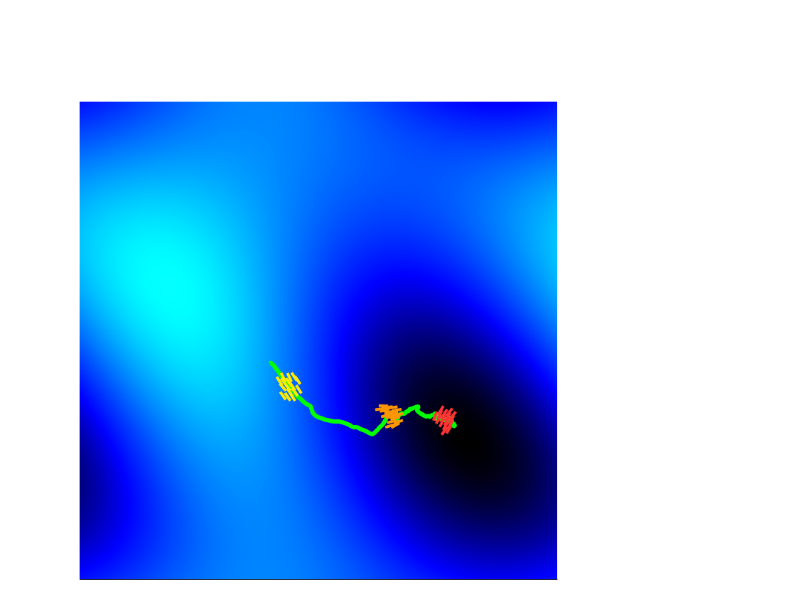
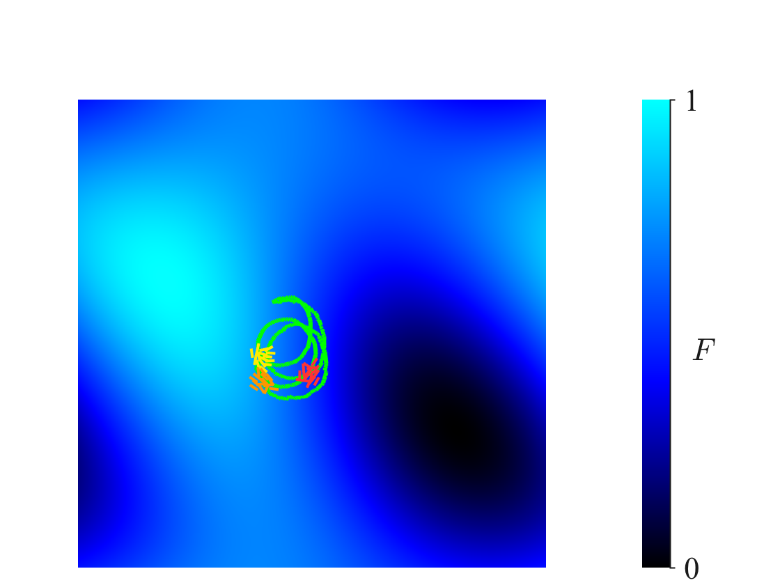
Typical trajectories of the model are depicted in Fig. 1. When the microscopic parameters are near optimal, the group readily finds a minimum of the field, as expected. For other parameters, by contrast, the group ceases to move or simply wanders, dissipating energy through random swarming motion without coherent direction. The success and efficiency of the collective fieldtaxis thus crucially depend on the microscopic parameters, .
The optimal efficiency can be found by a brute-force parameter search if there is only one continuous parameter characterizing the model or if parameters are discrete (see, e.g., Ref. Martínez-García et al. (2013)). As the number of parameters increases, however, such an approach quickly becomes intractable, with the requisite computational time roughly increasing as where is the desired accuracy and is the number of continuous parameters. For generic systems with multiple parameters, an alternative approach is thus imperative. We now demonstrate that a simple variant of reinforcement algorithms Sutton and Barto (1998), which have been applied to optimize behavior at an individual level Reddy et al. (2016); Colabrese et al. (2017), can be effective at a collective level.
Training Algorithm– Our training algorithm repeats the following protocol: cast a static field, initialize agents at , record the reward obtained up to time , and adjust parameters through reinforcement. These training sessions are indexed by .
Specifically, a light field is generated by defining
| (6) |
shifted and rescaled so that it ranges precisely from zero to one. Here the sum over wavevectors, , runs through and amplitudes and are independently drawn from a normal distribution foo (c). Agents are then initialized to positions uniformly within a circle of radius with a randomly chosen center. Velocities are in turn initialized to be .
In order to promote the decay of the average field intensity perceived by agents,
| (7) |
the reward is defined as
| (8) |
with a fixed terminal time . In other words, if decreases over time duration , the magnitude of its decrease is the reward; otherwise, there is no reward.
For each training, a pair of trial parameter values is chosen from the continuum of allowed values, and a reward is given probabilistically based on that choice. Our goal is to identify the pair of parameters, , that maximizes the average reward, which is equivalent to the continuum-armed bandit problem Agrawal (1995). This generalization of the classical multi-armed bandit problem Robbins (1952); Sutton and Barto (1998) has a simple learning algorithm that performs stochastic gradient ascent to shift the parameters toward optimality as the training proceeds Kleinberg (2005); Flaxman et al. (2005). Namely, at the -th training session with a light field and an initial configuration drawn as above, the rewards are evaluated at three nearby points in the parameter space: at , at , and at with deviation . The parameters are then updated as
| (9) | |||||
| (10) |
with foo (d). Over many iterations, these updates obtain an ascent in the landscape of the average reward function without evaluating such a function for every pair of parameters.
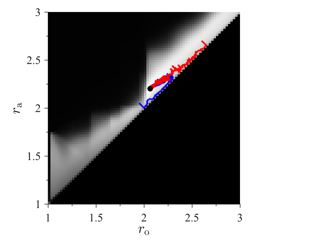
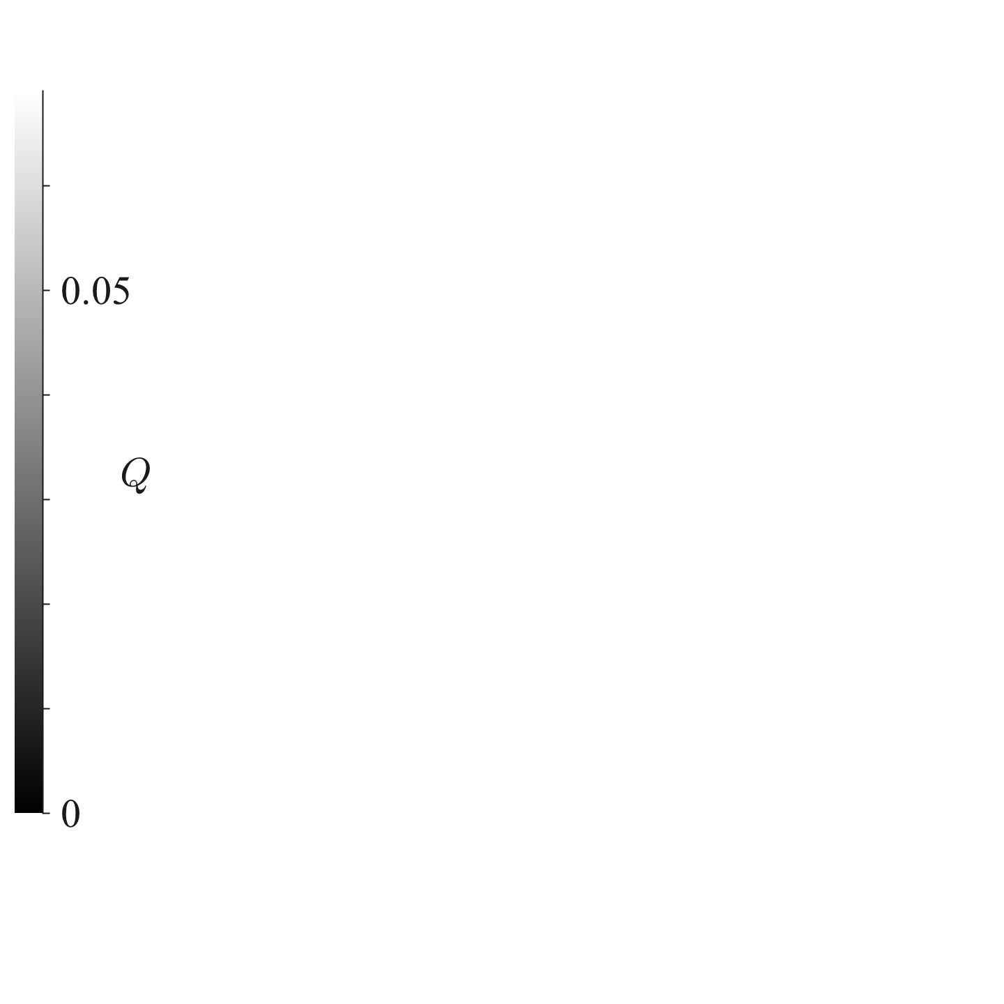
In Fig. 2 we depict training trajectories of the parameters with the terminal time for and , which sets the gradient scale to be roughly of order . The training has been carried out over sessions foo (a). Also depicted is the outcome of the brute-force parameter search, obtained with grid spacing in the range , at each point averaged over the realizations of local environments foo (a). The resultant error bars in are of order , barely sufficient to locate the optimum at this grid resolution. Bandit-algorithm trajectories converge to the optimum as long as initial guesses are chosen reasonably well, but with much less computational time and greater accuracy than the brute-force search. The bandit algorithm is further expected to scale better as the number of model parameters increases, with power-law dependence on Kleinberg (2005); Flaxman et al. (2005) in contrast to the exponential dependence of the brute-force search. The algorithm thus generalizes well.
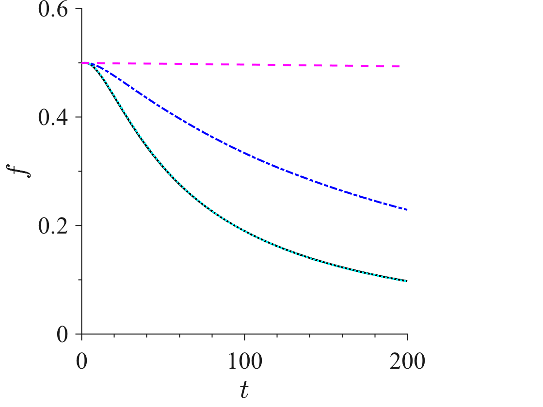
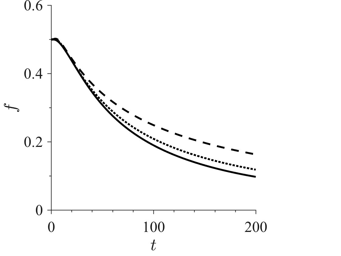
It is important to keep in mind that the choices of , , and affect the reward and hence the exact position of optimality. For instance, while the trained group maximizes decrease in the field intensity over time , some nearby parameters may – and indeed do – yield slightly better performance at other time scales [Fig. 1(c)]. Similarly, the optimal parameters shift as is varied, even though small-group training extends reasonably well upon scaling up group size (Fig. 3).
\sidesubfloat[]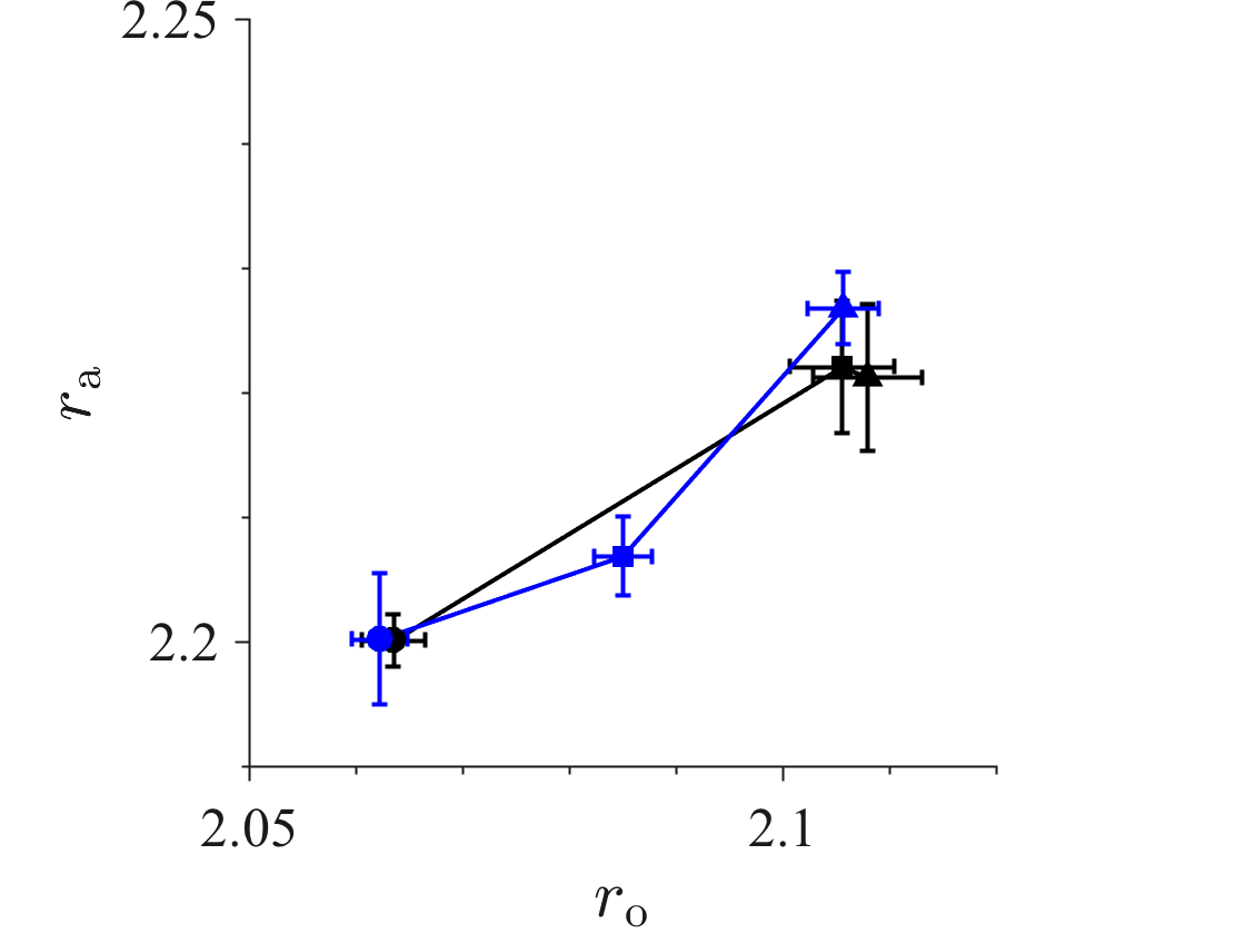 \sidesubfloat[]
Conclusion– In this paper, we have implemented a learning algorithm to optimize a specific reward for effective collective gradient sensing. Unlike some evolutionary algorithms that result in compromised optimality due to idiocy of selfish agents Torney et al. (2011); Hein et al. (2015); Bennati (2016); Torney et al. (2015); Kao et al. (2014), convergence to optimality is guaranteed for a reasonable initial guess. More broadly, this simple example suggests that machine-learning insights can be brought to bear on the optimization problems that arise in applications of swarm robotics.
We have further found that the optimality achieved depends on the choice of reward. A simplistic choice of reward and algorithm has been made here, especially in that there is no history dependence. If memory or history are taken into account, it might be possible to employ more elaborate and efficient reinforcement algorithms Watkins (1989); Watkins and Dayan (1992); Sutton and Barto (1998); Reddy et al. (2016); Colabrese et al. (2017). If, instead, exemplary motion trajectories to be mimicked are given, then we can use apprenticeship Abbeel and Ng (2004) or supervised learning, minimizing the deviation from such motions. In particular, we may be able to combine multiple collective swarming behaviors that belong to distinct species. This could lead us to the boundary of learning capability, as in self-assembly constructions Murugan et al. (2015a, b) and community detection Decelle et al. (2011); Zdeborová and Krzakala (2016); Moore (2017). In this regard, it is clear that the learning capability depends on the model used. Perhaps one can construct a general-purpose active matter model with many parameters that allows for fast and more generic learning, in the same vein as the deep-neural network that has been so successful in beating games such as Atari Mnih et al. (2015) and Go Silver et al. (2016).
Acknowledgements.
We thank Gordon J. Berman, Patrick Charbonneau, Iain D. Couzin, Daniel I. Goldman, Liesbeth M. C. Janssen, Stanley Kok, Joyjit Kundu, Arvind Murugan, and Daniel M. Sussman for stimulating discussions and suggestions. We also acknowledge the Duke Compute Cluster for computational times. This work was supported by grants from the National Science Foundation’s Research Triangle Materials Research Science and Engineering Center (No. DMR-1121107) and from the Simons Foundation (No. 454937, Patrick Charbonneau).References
- Allee (1931) W. C. Allee, Animal aggregations (The University of Chicago Press, 1931).
- Parrish and Edelstein-Keshet (1999) J. K. Parrish and L. Edelstein-Keshet, “Complexity, pattern, and evolutionary trade-offs in animal aggregation,” Science 284, 99 (1999).
- Camazine et al. (2001) S. Camazine, J.-L. Deneubourg, N.R. Franks, J. Sneyd, G. Theraulaz, and E. Bonabeau, Self-organization in biological systems (Princeton University Press, 2001).
- Krause and Ruxton (2002) J. Krause and G. D. Ruxton, Living in groups (Oxford University Press, 2002).
- Vicsek and Zafeiris (2012) T. Vicsek and A. Zafeiris, “Collective motion,” Phys. Rep. 517, 71 (2012).
- Marchetti et al. (2013) M. C. Marchetti, J. F. Joanny, S. Ramaswamy, T. B. Liverpool, J. Prost, M. Rao, and R. A. Simha, “Hydrodynamics of soft active matter,” Rev. Mod. Phys. 85, 1143 (2013).
- Cavagna and Giardina (2014) A. Cavagna and I. Giardina, “Bird flocks as condensed matter,” Annu. Rev. Condens. Matter Phys. 5, 183 (2014).
- Popkin (2016) G. Popkin, “The physics of life,” Nature 529, 16 (2016).
- Ögren et al. (2004) P. Ögren, E. Fiorelli, and N. E. Leonard, “Cooperative control of mobile sensor networks: Adaptive gradient climbing in a distributed environment,” IEEE Trans. Automat. Control 49, 1292 (2004).
- Hauert et al. (2011) S. Hauert, S. Leven, M. Varga, F. Ruini, A. Cangelosi, J.-C. Zufferey, and D. Floreano, “Reynolds flocking in reality with fixed-wing robots: communication range vs. maximum turning rate,” in Proceedings of International Conference on Intelligent Robots and Systems (IROS) (IEEE/RSJ, 2011) p. 5015.
- Martinoli et al. (2012) A. Martinoli, F. Mondada, N. Correll, G. Mermoud, M. Egerstedt, M. A. Hsieh, L. E. Parker, and K. Støy, Distributed Autonomous Robotic Systems: The 10th International Symposium, Vol. 83 (Springer, 2012).
- Bouffanais (2016) R. Bouffanais, Design and control of swarm dynamics (Springer, 2016).
- Heppner (1974) F. H. Heppner, “Avian flight formations,” Bird-Banding 45, 160 (1974).
- Heppner (1997) F. H. Heppner, “Three-dimensional structure and dynamics of bird flocks,” in Animal Groups in Three Dimensions, edited by J. K. Parrish and W. M. Hamner (Cambridge University Press, 1997) p. 68.
- Partridge and Pitcher (1980) B. L. Partridge and T. J. Pitcher, “The sensory basis of fish schools: relative roles of lateral line and vision,” J. Comp. Physiol. 135, 315 (1980).
- Partridge (1982) B. L. Partridge, “The structure and function of fish schools,” Sci. Am. 246, 114 (1982).
- Strogatz (2004) S. Strogatz, Sync: The emerging science of spontaneous order (Penguin UK, 2004).
- Hopfield (1982) J. J. Hopfield, “Neural networks and physical systems with emergent collective computational abilities,” Proc. Natl. Acad. Sci. U.S.A. 79, 2554 (1982).
- Reid et al. (2015) C. R. Reid, M. J. Lutz, S. Powell, A. B. Kao, I. D. Couzin, and S. Garnier, “Army ants dynamically adjust living bridges in response to a cost–benefit trade-off,” Proc. Natl. Acad. Sci. U.S.A. 112, 15113 (2015).
- Graham et al. (2017) J. M. Graham, A. B. Kao, D. A. Wilhelm, and S. Garnier, “Optimal construction of army ant living bridges,” bioRxiv , 116780 (2017).
- Werfel et al. (2014) J. Werfel, K. Petersen, and R. Nagpal, “Designing collective behavior in a termite-inspired robot construction team,” Science 343, 754 (2014).
- Farkas et al. (2002) I. Farkas, D. Helbing, and T. Vicsek, “Social behaviour: Mexican waves in an excitable medium,” Nature 419, 131 (2002).
- Silverberg et al. (2013) J. L. Silverberg, M. Bierbaum, J. P. Sethna, and I. Cohen, “Collective motion of humans in mosh and circle pits at heavy metal concerts,” Phys. Rev. Lett. 110, 228701 (2013).
- Janchar et al. (2000) T. Janchar, C. Samaddar, and D. Milzman, “The mosh pit experience: Emergency medical care for concert injuries,” Am. J. Emerg. Med. 18, 62 (2000).
- Selous (1931) E. Selous, Thought-Transference–or What?–in Birds. (Constable & Company, 1931).
- Aoki (1982) I. Aoki, “A simulation study on the schooling mechanism in fish,” Bull. Jpn. Soc. Sci. Fish. 48, 1081 (1982).
- Reynolds (1987) C. W. Reynolds, “Flocks, herds and schools: A distributed behavioral model,” ACM SIGGRAPH Comput. Graphics 21, 25 (1987).
- Vicsek et al. (1995) T. Vicsek, A. Czirók, E. Ben-Jacob, I. Cohen, and O. Shochet, “Novel type of phase transition in a system of self-driven particles,” Phys. Rev. Lett. 75, 1226 (1995).
- Couzin et al. (2002) I. D. Couzin, J. Krause, R. James, G. D. Ruxton, and N. R. Franks, “Collective memory and spatial sorting in animal groups,” J. Theor. Biol. 218, 1 (2002).
- Couzin (2007) I. D. Couzin, “Collective minds,” Nature 445, 715 (2007).
- Mitchell (1997) T. M. Mitchell, Machine Learning (McGraw-Hill, 1997).
- Sutton and Barto (1998) R. S. Sutton and A. G. Barto, Reinforcement learning: An introduction (MIT press, 1998).
- Rusell and Norvig (2003) S. J. Rusell and P. Norvig, Artificial intelligent: A modern approach (Prentice Hall, 2003).
- Koller and Friedman (2009) D. Koller and N. Friedman, Probabilistic graphical models: principles and techniques (MIT press, 2009).
- Murphy (2012) K. P. Murphy, Machine learning: a probabilistic perspective (MIT press, 2012).
- Goodfellow et al. (2016) I. Goodfellow, Y. Bengio, and A. Courville, Deep Learning (MIT Press, 2016).
- Engelmann (1881) Th. W. Engelmann, “Neue methode zur untersuchung der sauerstoffausscheidung pflanzlicher und thierischer organismen,” Pfluegers Arch. Gesamte Physiol. Menschen Tiere 25, 285 (1881).
- Pfeffer (1888) W. F. Pfeffer, “Über chemotaktische bewegungen von bacterien, flagellaten und volvocineen,” Untersuch. Bot. Inst. Tubingen 2, 582 (1888).
- Hong et al. (2007) Y. Hong, N. M. K. Blackman, N. D. Kopp, A. Sen, and D. Velegol, “Chemotaxis of nonbiological colloidal rods,” Phys. Rev. Lett. 99, 178103 (2007).
- Vergassola et al. (2007) M. Vergassola, E. Villermaux, and B. I. Shraiman, “‘Infotaxis’ as a strategy for searching without gradients,” Nature 445, 406 (2007).
- Berdahl et al. (2013) A. Berdahl, C. J. Torney, C. C. Ioannou, J. J. Faria, and I. D. Couzin, “Emergent sensing of complex environments by mobile animal groups,” Science 339, 574 (2013).
- Camley et al. (2016) B. A. Camley, J. Zimmermann, H. Levine, and W.-J. Rappel, “Emergent collective chemotaxis without single-cell gradient sensing,” Phys. Rev. Lett. 116, 098101 (2016).
- Sunyer et al. (2016) R. Sunyer, V. Conte, J. Escribano, A. Elosegui-Artola, A. Labernadie, L. Valon, D. Navajas, J. M. García-Aznar, J. J. Muñoz, P. Roca-Cusachs, and X. Trepat, “Collective cell durotaxis emerges from long-range intercellular force transmission,” Science 353, 1157 (2016).
- Wu et al. (2012) W. Wu, I. D. Couzin, and F. Zhang, “Bio-inspired source seeking with no explicit gradient estimation,” IFAC Proceedings Volumes 45, 240 (2012).
- (45) E. Luo, X. H. Fang, Y. Ng, and G. X. Gao, “Shinerbot: Bio-inspired collective robot swarm navigation platform,” .
- Katz et al. (2011) Y. Katz, K. Tunstrøm, C. C. Ioannou, C. Huepe, and I. D. Couzin, “Inferring the structure and dynamics of interactions in schooling fish,” Proc. Natl. Acad. Sci. U.S.A. 108, 18720 (2011).
- Bialek et al. (2012) W. Bialek, A. Cavagna, I. Giardina, T. Mora, E. Silvestri, M. Viale, and A. M. Walczak, “Statistical mechanics for natural flocks of birds,” Proc. Natl. Acad. Sci. U.S.A. 109, 4786 (2012).
- Cavagna et al. (2014) A. Cavagna, I. Giardina, F. Ginelli, T. Mora, D. Piovani, R. Tavarone, and A. M. Walczak, “Dynamical maximum entropy approach to flocking,” Phys. Rev. E 89, 042707 (2014).
- Nguyen et al. (2017) H. C. Nguyen, R. Zecchina, and J. Berg, “Inverse statistical problems: from the inverse Ising problem to data science,” (2017), arXiv:1702.01522 [cond-mat.dis-nn] .
- foo (a) Since the system size is large enough, in order to sample over many local environments, we have prepared independent light fields and recycled over them with different initial positions of agents.
- foo (b) When the noise level is set to zero, the entire group sometimes comes to a complete halt.
- Martínez-García et al. (2013) R. Martínez-García, J. M. Calabrese, T. Mueller, K. A. Olson, and C. López, “Optimizing the search for resources by sharing information: Mongolian gazelles as a case study,” Phys. Rev. Lett. 110, 248106 (2013).
- Reddy et al. (2016) G. Reddy, A. Celani, T. J. Sejnowski, and M. Vergassola, “Learning to soar in turbulent environments,” Proc. Natl. Acad. Sci. U.S.A. , 201606075 (2016).
- Colabrese et al. (2017) S. Colabrese, K. Gustavsson, A. Celani, and L. Biferale, “Flow navigation by smart microswimmers via reinforcement learning,” Phys. Rev. Lett. 118, 158004 (2017).
- foo (c) The result does not depend on the mean and variance of the Gaussian distribution upon rescaling.
- Agrawal (1995) R. Agrawal, “The continuum-armed bandit problem,” SIAM J. Control and Optimization 33, 1926 (1995).
- Robbins (1952) H. Robbins, “Some aspects of the sequential design of experiments,” Bull. Amer. Math. Soc. 58, 527 (1952).
- Kleinberg (2005) R. D. Kleinberg, “Nearly tight bounds for the continuum-armed bandit problem,” in Advances in Neural Information Processing Systems 17 (MIT Press, 2005) p. 697.
- Flaxman et al. (2005) A. D. Flaxman, A. T. Kalai, and H. B. McMahan, “Online convex optimization in the bandit setting: gradient descent without a gradient,” in Proceedings of the sixteenth annual ACM-SIAM symposium on Discrete algorithms (SIAM, 2005) p. 385.
- foo (d) When the update takes the parameters outside the region , they are further shifted to .
- Torney et al. (2011) C. J. Torney, A. Berdahl, and I. D. Couzin, “Signalling and the evolution of cooperative foraging in dynamic environments,” PLoS Comput. Biol. 7, e1002194 (2011).
- Hein et al. (2015) A. M. Hein, S. B. Rosenthal, G. I. Hagstrom, A. Berdahl, C. J. Torney, and I. D. Couzin, “The evolution of distributed sensing and collective computation in animal populations,” Elife 4, e10955 (2015).
- Bennati (2016) S. Bennati, “On the role of collective sensing and evolution in group formation,” (2016), arXiv:1602.06737 [q-bio.PE] .
- Torney et al. (2015) C. J. Torney, T. Lorenzi, I. D. Couzin, and S. A. Levin, “Social information use and the evolution of unresponsiveness in collective systems,” J. Royal Soc. Interface 12, 20140893 (2015).
- Kao et al. (2014) A. B. Kao, N. Miller, C. Torney, A. Hartnett, and I. D. Couzin, “Collective learning and optimal consensus decisions in social animal groups,” PLoS Comput. Biol. 10, e1003762 (2014).
- Watkins (1989) C. J. C. H. Watkins, Learning from delayed rewards, Ph.D. thesis, King’s College, Cambridge (1989).
- Watkins and Dayan (1992) C. J. C. H. Watkins and P. Dayan, “Q-learning,” Mach. Learn. 8, 279 (1992).
- Abbeel and Ng (2004) P. Abbeel and A. Y. Ng, “Apprenticeship learning via inverse reinforcement learning,” in Proceedings of the twenty-first international conference on Machine learning (ACM, 2004) p. 1.
- Murugan et al. (2015a) A. Murugan, Z. Zeravcic, M. P. Brenner, and S. Leibler, “Multifarious assembly mixtures: Systems allowing retrieval of diverse stored structures,” Proc. Natl. Acad. Sci. U.S.A. 112, 54 (2015a).
- Murugan et al. (2015b) A. Murugan, J. Zou, and M. P. Brenner, “Undesired usage and the robust self-assembly of heterogeneous structures,” Nat. Commun. 6, 6203 (2015b).
- Decelle et al. (2011) A. Decelle, F. Krzakala, C. Moore, and L. Zdeborová, “Inference and phase transitions in the detection of modules in sparse networks,” Phys. Rev. Lett. 107, 065701 (2011).
- Zdeborová and Krzakala (2016) L. Zdeborová and F. Krzakala, “Statistical physics of inference: Thresholds and algorithms,” Adv. Phys. 65, 453 (2016).
- Moore (2017) C. Moore, “The computer science and physics of community detection: landscapes, phase transitions, and hardness,” (2017), arXiv:1702.00467 [cs.CC] .
- Mnih et al. (2015) V. Mnih, K. Kavukcuoglu, D. Silver, A. A. Rusu, J. Veness, M. G. Bellemare, A. Graves, M. Riedmiller, A. K. Fidjeland, G. Ostrovski, S. Petersen, C. Beattie, A. Sadik, I. Antonoglou, H. King, D. Kumaran, D. Wierstra, S. Legg, and D. Hassabis, “Human-level control through deep reinforcement learning,” Nature 518, 529 (2015).
- Silver et al. (2016) D. Silver, A. Huang, C. J. Maddison, A. Guez, L. Sifre, G. Van Den Driessche, J. Schrittwieser, I. Antonoglou, V. Panneershelvam, M. Lanctot, S. Dieleman, D. Grewe, J. Nham, N. Kalchbrenner, I. Sutskever, T. Lillicrap, M. Leach, K. Kavukcuoglu, T. Graepel, and D. Hassabis, “Mastering the game of go with deep neural networks and tree search,” Nature 529, 484 (2016).