Rank-Select Indices Without Tears

Abstract

A rank-select index for a sequence $B=(b_{1},\ldots,b_{n})$ of $n$ bits, where $n\in\mathbb{N}=\{1,2,\ldots\}$, is a data structure that, if provided with an operation to access $\Theta(\log n)$ arbitrary consecutive bits of $B$ in constant time (thus $B$ is stored outside of the data structure), can compute $\hbox{{rank\/}}_{B}(j)=\sum_{i=1}^{j}b_{i}$ for given $j\in\{0,\ldots,n\}$ and $\hbox{{select\/}}_{B}(k)=\min\{j\in\mathbb{N}\mid\hbox{{rank\/}}_{B}(j)\geq k\}$ for given $k\in\{1,\ldots,\sum_{i=1}^{n}b_{i}\}$. We describe a new rank-select index that, like previous rank-select indices, occupies $O({{n\log\log n}/{\log n}})$ bits and executes rank and select queries in constant time. Its derivation is intended to be particularly easy to follow and largely free of tedious low-level detail, its operations are given by straight-line code, and we show that it can be constructed in $O({n/{\log n}})$ time.

1 Introduction

When $S$ is a finite multiset of integers and $j\in\mathbb{Z}=\{\ldots,-1,0,1,\ldots\}$, we write $\hbox{{rank\/}}_{S}(j)$ for the rank of $j$ in $S$, i.e., $\hbox{{rank\/}}_{S}(j)=|\{i\in S:i\leq j\}|$. Moreover, for each $k\in\{1,\ldots,|S|\}$, $\hbox{{select\/}}_{S}(k)=\min\{j\in\mathbb{Z}:\hbox{{rank\/}}_{S}(j)\geq k\}$. If the elements of $S$ are arranged in nondecreasing order in positions $1,\ldots,|S|$, then $\hbox{{rank\/}}_{S}(j)$ is the largest position of an element $\leq j$ (0 if there is no such element), for $j\in\mathbb{Z}$, and $\hbox{{select\/}}_{S}(k)$ is the element in position $k$, for $k\in\{1,\ldots,|S|\}$.

The operations rank and select are also defined for bit sequences. If $B=(b_{1},\ldots,b_{n})$ is a sequence of $n$ bits, for some $n\in\mathbb{N}=\{1,2,\ldots\}$, then $\hbox{{rank\/}}_{B}(j)=\sum_{i=1}^{j}b_{i}$ for $j\in\{0,\ldots,n\}$ and, again, $\hbox{{select\/}}_{B}(k)=\min\{j\in\mathbb{N}:\hbox{{rank\/}}_{B}(j)\geq k\}$ for $k\in\{1,\ldots,\sum_{i=1}^{n}b_{i}\}$. The connection between the two definitions is close: If a simple set $S$ is a subset of $\{a,\ldots,a+n-1\}$ for some known $a\in\mathbb{Z}$ and $n\in\mathbb{N}$, $S$ can be represented via the bit sequence $(b_{1},\ldots,b_{n})$ with $b_{i}=1\Leftrightarrow a-1+i\in S$, for $i=1,\ldots,n$. In this case we say that $S$ is given by its bit-vector representation over the universe $\{a,\ldots,a+n-1\}$ or with offset $a$ and span $n$. Clearly $\hbox{{rank\/}}_{S}(j)=\hbox{{rank\/}}_{B}(j-(a-1))$ for $j\in\{a-1,\ldots,a-1+n\}$ and $\hbox{{select\/}}_{S}(k)=a-1+\hbox{{select\/}}_{B}(k)$ for $k\in\{1,\ldots,|S|\}$. Answering rank and select queries about a simple set of integers therefore reduces to answering rank and select queries about its bit-vector representation with some known offset and span.

A (static) rank-select structure for a sequence $B=(b_{1},\ldots,b_{n})$ of $n$ bits, for some $n\in\mathbb{N}$, is a data structure capable of returning $\hbox{{rank\/}}_{B}(j)$ for arbitrary given $j\in\{0,\ldots,n\}$ and $\hbox{{select\/}}_{B}(k)$ for arbitrary given $k\in\{1,\ldots,\sum_{i=1}^{n}b_{i}\}$. A data structure that can answer the same queries, but only if provided with an operation to access $\Theta(\log n)$ arbitrary consecutive bits of $B$ in constant time (thus $B$ is stored outside of the data structure), is known as a rank-select index for $B$. We call $B$ the client sequence of a rank-select structure or index for $B$. Rank-select structures and indices are of fundamental importance in space-efficient computing, have been studied extensively since the 1970s, and have many and diverse applications. Elias [3] considered the representation of multisets of integers in the context of data retrieval. For a multiset $S$, his direct or table-lookup question corresponds to $\hbox{{select\/}}_{S}$, and his inverse question is closely related to $\hbox{{rank\/}}_{S}$. Jacobson, who introduced the terms rank and select [9, 10], used rank-select structures to represent trees and graphs in little space while still permitting their efficient traversal. Along the way, he solved the problem of finding matching parentheses in a balanced sequence of parentheses, again with rank-select structures as crucial components of the overall data structure. Rank-select structures and indices have also found applications in areas such as string processing [6], computational geometry [11] and graph algorithms [8].

Jacobson designed a rank-select index for bit sequences of length $n\in\mathbb{N}$ that occupies $O({{n\log\log n}/{\log n}})$ bits and answers rank queries in constant time. While he was unable to obtain a constant-time select operation, this was remedied by Clark [2], at the price of a somewhat higher space bound. From now on we will be interested only in rank-select structures and indices that answer all queries in constant time; for ease of discussion, consider this property to be part of their definition.

A rank-select index that uses $O({{n\log\log n}/{\log n}})$ bits was described by Raman, Raman and Satti [13, Lemma 4.1]. A matching lower bound of $\Omega({{n\log\log n}/{\log n}})$ on the number of bits needed by a rank-select index that accesses only $O(\log n)$ bits of its client sequence during the processing of a query was proved by Golynski [5]. Thus a rank-select structure for a sequence $B$ of $n$ bits that consists of $B$ plus a suitable index must occupy $n+\Omega({{n\log\log n}/{\log n}})$ bits. While this is a natural way of organizing a rank-select structure, Pǎtraşcu [12] proved the interesting fact that there are smaller rank-select structures that do not store $B$ in its “raw” form.

In this paper we describe another $O({{n\log\log n}/{\log n}})$-bit rank-select index. While previous descriptions of rank-select structures and indices abund with ad-hoc and rather tedious low-level detail, we aim for a more systematic and high-level approach based largely on pictures that leads to the optimal result with little effort on the part of the reader. Our rank-select index offers the first select operation that can be formulated as a piece of straight-line code, i.e., its implementation is free of tests and branching (in one place, fulfilling this promise involves a small amount of “cheating”, as will be explained later). We also consider the problem of efficient construction of rank-select indices, an aspect that was ignored in much previous research but is essential to many applications. Our main result is the following:

Theorem 1.1.

For every $n\in\mathbb{N}$ and for every sequence $B$ of $n$ bits, given in the form of a stream of $O({n/{\log n}})$ chunks of $O({{n\log\log n}/{\log n}})$ consecutive bits each, a rank-select index for $B$ that executes $\hbox{{rank\/}}_{B}$ and $\hbox{{select\/}}_{B}$ in constant time and occupies $O({{n\log\log n}/{\log n}})$ bits can be constructed in $O({n/{\log n}})$ time using $O({{n\log\log n}/{\log n}})$ bits of working memory.

The theorem insists that the client sequence $B$ be provided in several chunks because the available working space does not allow us to store $B$ in its entirety. Typically $B$ would be provided in $\Theta({n/{\log n}})$ chunks of $O(\log n)$ bits each. If $B$ is stored in random-access read-only memory, of course, it is trivial to produce the necessary chunks, but the theorem implies that the construction of the rank-select index does not require random access to $B$ and can make do with a single pass over $B$.

Our model of computation is a word RAM [1, 7] with a word length of $w=\Omega(\log n)$ bits, where $w$ is assumed large enough to allow all memory words in use to be addressed. The word RAM has constant-time operations for addition, subtraction and multiplication modulo $2^{w}$, division with truncation ($(x,y)\mapsto\lfloor{x/y}\rfloor$ for $y>0$), left shift modulo $2^{w}$ ($(x,y)\mapsto(x\ll y)\bmod 2^{w}$, where $x\ll y=x\cdot 2^{y}$), right shift ($(x,y)\mapsto x\gg y=\lfloor{x/{2^{y}}}\rfloor$), and bitwise Boolean operations (and, or and xor (exclusive or)).

2 Ingredients of the New Rank-Select Index

Our overall approach, shared with earlier solutions, is to break down a given instance of the rank-select problem, i.e., the problem of answering rank and select queries for a given bit sequence or multiset, into still smaller instances, eventually arriving at instances so tiny that they can be solved by brute force, i.e., table lookup. We provide a bottom-up description, proceeding from table lookup via basic reductions of instances of the rank-select problem to simpler instances and ending with the complete rank-select index that reduces rank and select queries about the client sequence all the way to table lookup. We prefer to phrase much of the discussion in terms of (multi)sets rather than bit sequences. The tables needed by the rank-select index and their computation are discussed in the next subsection.

2.1 Table Lookup

This subsection describes three different variants, denoted T1–T3, of the table-lookup method, as applied to the rank-select problem. In our applications, the parameters $N$ and $M$ for variants T2 and T3 will be so small as to render negligible the space occupied by the tables and the time needed to compute them.

T1.

In order to answer $\hbox{{rank\/}}_{S}$ and $\hbox{{select\/}}_{S}$ queries about one particular subset $S$ of $\{1,\ldots,N\}$, where $N\in\mathbb{N}$ is known, we can simply store a table of $\hbox{{rank\/}}_{S}(j)$ for $j=0,\ldots,N$ and $\hbox{{select\/}}_{S}(k)$ for $k=1,\ldots,|S|$ and answer a query by returning an appropriate table entry. The number of bits needed is $O(N\log N)$, and the table can be computed in $O(N)$ time from a bit-vector representation of $S$.

T2.

If the goal is to answer $\hbox{{rank\/}}_{S}$ and $\hbox{{select\/}}_{S}$ queries, where $S$ now is also specified in the query and can be an arbitrary subset of $\{1,\ldots,N\}$, we can create a subtable as for variant T1 for each of the $2^{N}$ possible subsets $S$ and store the $2^{N}$ subtables, each indexed by the bit-vector representation over $\{1,\ldots,N\}$ of the corresponding set $S$, in a table of $O(2^{N}N\log N)$ bits whose computation takes $O(2^{N}N)$ time.

T3.

If $S$ is a variable subset of $\{1,\ldots,N\}$ but known to be of size at most $M$ for some given $M\in\mathbb{N}$, $S$ can be represented as an $M$-tuple of integers in $\{1,\ldots,N\}$ by first listing the elements of $S$ and then, if $|S|<M$, repeating the last element. Each of the $M$ integers can in turn be represented in $\lceil\log_{2}\!N\rceil$ bits. Since $2^{\lceil\log_{2}\!N\rceil}\leq 2N$, this gives us an alternative to variant T2 with a table of $O((2N)^{M+1}\log N)$ bits that can be computed in $O((2N)^{M+1})$ time.

2.2 Three Basic Reductions

Let $g$ be a nondecreasing function from $\mathbb{Z}$ to $\mathbb{Z}$ (informally, the grouping function) with the property that $g^{-1}(q)=\{i\in\mathbb{Z}\mid g(i)=q\}$ is finite for all $q\in\mathbb{Z}$ and let $S$ be a finite multiset of integers. While $g(S)$ as usual denotes the simple set $\{q\in\mathbb{Z}\mid S\cap g^{-1}(q)\not=\emptyset\}$, we write $g(\mskip-3.0mu(S)\mskip-3.0mu)$ for the multiset $\{g(i)\mid i\in S\}$, in which each $q\in\mathbb{Z}$ occurs with multiplicity $|S\cap g^{-1}(q)|$. For $j\in\mathbb{Z}$, it is clear that, with $q=g(j)$,

$$\hbox{{rank\/}}_{S}(j)=\hbox{{rank\/}}_{g(\mskip-3.0mu(S)\mskip-3.0mu)}(q-1)+\hbox{{rank\/}}_{S\cap g^{-1}(q)}(j),$$ (1)

since the terms $\hbox{{rank\/}}_{g(\mskip-3.0mu(S)\mskip-3.0mu)}(q-1)$ and $\hbox{{rank\/}}_{S\cap g^{-1}(q)}(j)$ count the elements $i$ of $\{i\in S:i\leq j\}$ with $g(i)<q$ and with $g(i)=q$, respectively. Furthermore, for $k\in\{1,\ldots,|S|\}$, $g(\hbox{{select\/}}_{S}(k))=\hbox{{select\/}}_{g(\mskip-3.0mu(S)\mskip-3.0mu)}(k)$ and therefore, with $q=\hbox{{select\/}}_{g(\mskip-3.0mu(S)\mskip-3.0mu)}(k)$,

$$\hbox{{select\/}}_{S}(k)=\hbox{{select\/}}_{S\cap g^{-1}(q)}(k-\hbox{{rank\/}}_{g(\mskip-3.0mu(S)\mskip-3.0mu)}(q-1)),$$ (2)

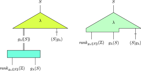
since $\hbox{{rank\/}}_{g(\mskip-3.0mu(S)\mskip-3.0mu)}(q-1)$ again is the number of elements $i\in S$ with $g(i)<q$, so that, if $S$ is presented in sorted order in $|S|$ positions, $\hbox{{select\/}}_{S}(k)$ is the element in position $k-\hbox{{rank\/}}_{g(\mskip-3.0mu(S)\mskip-3.0mu)}(q-1)$ among the elements with the same value under $g$ as itself, i.e., within $S\cap g^{-1}(q)$. Let us use $(S|g)$ as a convenient notation for the function $(g_{|S})^{-1}$ that maps each $q\in\mathbb{Z}$ to $S\cap g^{-1}(q)$. Then answering rank and select queries about $S$ in constant time reduces to answering rank and select queries about $g(\mskip-3.0mu(S)\mskip-3.0mu)$ and about values of $(S|g)$ in constant time. For brevity, we express this by saying that $S$ reduces to $g(\mskip-3.0mu(S)\mskip-3.0mu)$ and $(S|g)$. We will use this only with $g=g_{\lambda}$ for some $\lambda\in\mathbb{N}$, where $g_{\lambda}(i)=\lfloor i/\lambda\rfloor$ for all $i\in\mathbb{Z}$, and call $\lambda$ the parameter of the reduction. Variations of this reduction have been used since the early days of rank-select indices [9, 10]. We call it BR1 (“basic reduction 1”) and denote it symbolically with a triangular shape, as shown in the left subfigure of Fig. 1: $S$, at the apex of the triangle, reduces to $g_{\lambda}(\mskip-3.0mu(S)\mskip-3.0mu)$ and $(S|g_{\lambda})$ at its base. The double line serves as a reminder that $g_{\lambda}(\mskip-3.0mu(S)\mskip-3.0mu)$ in general is a multiset even if $S$ is not, and a bar through the line to $(S|g_{\lambda})$ indicates that $(S|g_{\lambda})$ is a set-valued function rather than just a set. We refrain from connecting $S$ to the triangle with a double line because we will use the reduction only for simple sets $S$.

Figure 1: The three basic reductions BR1–BR3.

Denote by $\hbox{{supp\/}}(S)$ the support of the multiset $S$, i.e., the simple set that contains exactly the same values as $S$, but each value only once, and let $\hbox{{rank\/}}_{S}(\mathbb{Z})$ be the image of the $\hbox{{rank\/}}_{S}$ function. For example, with $S=\{1,1,2,4,4,4\}$ we have $\hbox{{supp\/}}(S)=\{1,2,4\}$ and $\hbox{{rank\/}}_{S}(\mathbb{Z})=\{0,2,3,6\}$. A second reduction is given by the formulas

$$\hbox{{rank\/}}_{S}(j) =\hbox{{select\/}}_{\hbox{{rank\/}}_{S}(\mathbb{Z})}(\hbox{{rank\/}}_{\hbox{{supp\/}}(S)}(j)+1)\mbox{\quad and}$$ (3)

$$\hbox{{select\/}}_{S}(k) =\hbox{{select\/}}_{\hbox{{supp\/}}(S)}(\hbox{{rank\/}}_{\hbox{{rank\/}}_{S}(\mathbb{Z})}(k-1)),$$ (4)

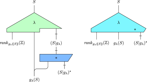
for $j\in\mathbb{Z}$ and $k\in\{1,\ldots,|S|\}$. To see the validity of the first formula, whose origins can be traced back to Fano [4, Step 2], note that the $(q+1)$st smallest element of $\hbox{{rank\/}}_{S}(\mathbb{Z})$, for $q=0,\ldots,|\hbox{{supp\/}}(S)|$, is the total number of occurrences in $S$ of the $q$ smallest distinct values in $S$. With $q=\hbox{{rank\/}}_{\hbox{{supp\/}}(S)}(j)$, this is precisely $\hbox{{rank\/}}_{S}(j)$. The second formula is implied by the following observation: If $S$, presented in sorted order in $|S|$ positions, is thought of as partitioned into maximal ranges of occurrences of the same value, then $\hbox{{rank\/}}_{\hbox{{rank\/}}_{S}(\mathbb{Z})}(k-1)$ is one more than the number of ranges that end strictly before the $k$th position. Thus $S$ also reduces to $\hbox{{rank\/}}_{S}(\mathbb{Z})$ and $\hbox{{supp\/}}(S)$. We call this reduction BR2 and depict it as shown in the middle subfigure of Fig. 1.

Denote by $(S|g)^{*}$ the function defined on $\{1,\ldots,|g(S)|\}$ that maps $q$ to $(S|g)(\hbox{{select\/}}_{g(S)}(q))$, for $q=1,\ldots,|g(S)|$. Informally, if $(S|g)$ is thought of as a list of subsets of $S$, then $(S|g)^{*}$ is the sublist that contains only the nonempty subsets. Clearly, for $q\in\mathbb{Z}$,

$$(S|g)(q)=\begin{cases}(S|g)^{*}(\hbox{{rank\/}}_{g(S)}(q)),&\mbox{ if }q\in g(S),\cr\emptyset,&\mbox{ otherwise}.\cr\end{cases}$$ (5)

Since we can test whether $q\in g(S)$ by evaluating $\hbox{{rank\/}}_{g(S)}(q)-\hbox{{rank\/}}_{g(S)}(q-1)$, which is 1 if $q\in g(S)$ and 0 otherwise, $(S|g)$ (i.e., $(S|g)(q)$ for each $q\in\mathbb{Z}$) reduces to $g(S)$ and $(S|g)^{*}$. This third and last basic reduction, BR3, is depicted in the right subfigure of Fig. 1.

2.3 Two Combined Reductions

We can combine BR1 and BR2 as illustrated in Fig. 2. This yields a reduction, CR1, of $S$ to $\hbox{{rank\/}}_{g_{\lambda}(\mskip-3.0mu(S)\mskip-3.0mu)}(\mathbb{Z})$, $\hbox{{supp\/}}(g_{\lambda}(\mskip-3.0mu(S)\mskip-3.0mu))=g_{\lambda}(S)$, and $(S|g_{\lambda})$. Incorporating also BR3, we obtain a second combined reduction, CR2, shown in Fig. 3.

Figure 2: The first combined reduction CR1. Left: Internal structure. Right: Pictorial representation.

Figure 3: The second combined reduction CR2. Left: Internal structure. Right: pictorial representation.

In the concrete rank-select index, sets of integers are represented as bit vectors with convenient offsets and spans. The offsets and spans are not stored with every set, but calculated in parallel with the application of reductions according to the following rules:

The client sequence $B$, prefixed by a 0 (see later), is viewed as representing a set with offset 0 and span $|B|+1$. Recursively, if a set $S$ has offset $a$ and span $n$ and $m=|S|$, then

• $\hbox{{rank\/}}_{g_{\lambda}(\mskip-3.0mu(S)\mskip-3.0mu)}(\mathbb{Z})$ has offset 0, span $m+1$ and size at most $\lceil n/\lambda\rceil+1$.

• $g_{\lambda}(S)$ has offset $g_{\lambda}(a)$, span $\lceil n/\lambda\rceil+1$ and size at most $m$.

• $(S|g_{\lambda})(q)$ has offset $\lambda q$ and span $\lambda$ for all $q\in\mathbb{Z}$.

• $(S|g_{\lambda})^{*}(q)$ has offset $\lambda\cdot\hbox{{select\/}}_{g_{\lambda}(S)}(q)$ and span $\lambda$ for all $q\in\{1,\ldots,|g_{\lambda}(S)|\}$.

Using the rules to keep track of offsets and spans enables us, at the bottom of a recursive application of reductions, to translate queries about sets correctly to queries about their bit-vector representations with the given offsets and spans. So as not to clutter the description, this simple translation will not be formulated explicitly.

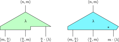
The effect of each type of combined reduction on spans and sizes is depicted in Fig. 4. A pair of the form $\langle n,m\rangle$ indicates that a set has span $n$ and size at most $m$, except that the rounding to integer values and the occasional ${}+1$ were ignored. When we refrain from bounding the size of a set by anything better than its span, $\langle n\rangle$ is used as an abbreviation for $\langle n,n\rangle$. If $S$ has offset $a$ and span $n$, $(S|g_{\lambda})(q)$ can be nonempty only if $q$ belongs to the set $\{g_{\lambda}(a),\ldots,g_{\lambda}(a+n-1)\}$ of size at most $\lceil\frac{n}{\lambda}\rceil+1$, which motivates the label $\frac{n}{\lambda}\cdot\langle\lambda\rangle$ in the left subfigure. In terms of the concrete data structure, the expression $\frac{n}{\lambda}\cdot\langle\lambda\rangle$ should be thought of as indicating an array of (approximately) $\frac{n}{\lambda}$ subordinate data structures, each of which is for a set of span $\lambda$. $(S|g)^{*}(q)$ is defined only for $1\leq q\leq|g(S)|\leq|S|$, which motivates the label $m\cdot\langle\lambda\rangle$ in the right subfigure.

Figure 4: The approximate effect of the two combined reductions CR1 and CR2 on $\langle\mbox{span},\mbox{size}\rangle$.

The new optimal rank-select index can be pieced together with little effort from a constant number of instances of the combined reductions CR1 and CR2. As a warm-up and to familiarize the reader with the approach and the notation, we first develop a simpler rank-select structure that occupies $\Theta(n)$ bits for client sequences of $n$ bits.

3 A Simplified $O(n)$-Bit Rank-Select Structure

The simplified rank-select structure is best thought of as the tree $T_{\mbox{\scriptsize S}}$ shown in Fig. 5 annotated with $\langle\mbox{rank},\mbox{size}\rangle$ pairs suitable for a client sequence of $n$ bits. Each inner node in $T_{\mbox{\scriptsize S}}$ corresponds to an instance of the composite reduction CR1 (for brevity, is a CR1-node) and is drawn with the characteristic shape of that reduction. Each leaf in $T_{\mbox{\scriptsize S}}$ corresponds to an instance or an array of instances of one of the variants of the table-lookup method and is drawn as a rectangle labeled with the name of the relevant variant. During the execution of a query, each inner node in $T_{\mbox{\scriptsize S}}$ applies its associated reduction and each leaf answers queries using its table-lookup variant.

Figure 5: A simplified rank-select structure that uses $O(n)$ bits.

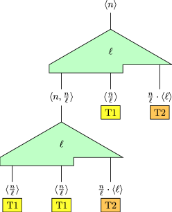
The reductions in $T_{\mbox{\scriptsize S}}$ both use a parameter $\ell\in\mathbb{N}$. Here and in the following, we choose $\ell=\Theta(\log n)$ such that the cost, in terms of time and space, of the table needed by table-lookup variant T2 with $N=\ell$ is negligible. In concrete terms, we take this to mean that $2^{\ell}\ell\log\ell=O({n/\log n})$, which is certainly satisfied if $\ell\leq({1/2)}\log_{2}n$.

The simplified rank-select structure is correct by construction and trivially executes queries in constant time. Let us analyze its storage requirements, for the time being ignoring rounding issues and pretending that the expressions for spans and sizes in Fig. 4 are exact. The first step is to verify that the $\langle\mbox{span},\mbox{size}\rangle$ pairs in Fig. 5 have indeed be calculated in accordance with Fig. 4. Each node in $T_{\mbox{\scriptsize S}}$ needs to store a constant number of offsets, spans and other integers that allow it to access arrays and bit sequences correctly. Beyond this, inner nodes have no associated storage. Each leaf that uses table-lookup variant T1 (is a T1-leaf, say) stores a table of rank and select for a sequence of $\frac{n}{\ell}$ bits, which needs $O(\frac{n}{\ell}\log n)=O(n)$ bits. Similarly, each T2-leaf stores an array of $\frac{n}{\ell}$ sequences, each of $\ell$ bits, again for a total of $O(n)$ bits. Adding the $O({n/\log n})$ bits occupied by a global table for variant T2 and $O(\log n)$ bits for a constant number of offsets, spans and other integers, we arrive at a grand total of $O(n)$ bits. It is easy to see that the error incurred by the approximation involved in Fig. 4 amounts to less than a constant factor (this is because error terms bounded by constants affect only quantities that are $\Omega(\log n)$), so that the true number of bits used by the simplified rank-select structure is also $O(n)$.

4 The New Optimal Rank-Select Index

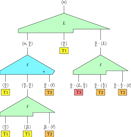
The new optimal rank-select index has much in common with the simplified rank-select structure of the previous section. In order to achieve a better space bound, however, the optimal index must comprise a few additional reductions. Its structure is given by the tree $T$ shown in Fig. 6. While most reductions use the parameter $\ell$ with $\ell=\Theta(\log n)$ introduced in Section 3, the reduction at the root of $T$ employs a larger parameter $L\in\mathbb{N}$. We choose $L=\Theta({{(\log n)^{2}}/{\log\log n}})$ as a multiple of $\ell$ such that the cost of the table needed by table-lookup variant T3 with $N=L+1$ and $M=1+{L/\ell}$ is negligible. In concrete terms, we take this to mean that $(2(L+1))^{2+{L/\ell}}\log L=O({n/\log n})$, which is ensured if ${L/\ell}\leq({1/4}){{\log_{2}\!n}/{\log_{2}\!\log_{2}\!n}}$.

Figure 6: The new optimal rank-select index.

4.1 Analysis of the Space Requirements

As in the case of the simplified rank-select structure, the optimal rank-select index is correct by construction and trivially executes queries in constant time. Because we now aim for a space bound of $o(n)$ bits, we must pay special attention to the rightmost leaf in the tree $T$ with its (approximately) $\frac{n}{L}\cdot\frac{L}{\ell}=\frac{n}{\ell}$ sequences, each of (at most) $\ell$ bits. As is not difficult to see, each of the relevant bit sequences is a subsequence of the client sequence $B$, so that there is no need to store any data in the rightmost leaf—it suffices to provide it with constant-time access to arbitrary subsequences of at most $\ell=\Theta(\log n)$ consecutive bits in $B$, which is precisely what the rank-select index is allowed to rely on.

The remaining part of the analysis of the space requirements parallels what was done in Section 3 for the simplified rank-select structure, and again we can pretend that the expressions given in Fig. 4 are exact—as a minor exception, one should observe that table-lookup variant T3 is indeed used with $N=L+1$ and $M=1+{L/\ell}$. Again, the first step is to verify that the $\langle\mbox{span},\mbox{size}\rangle$ pairs in Fig. 6 have been calculated in accordance with Fig. 4.

Each T1-leaf holds tables of rank and select for bit sequences of length $\frac{n}{L}$ or $\frac{n}{\ell^{2}}$. The number of bits needed for the tables is therefore $O((\frac{n}{L}+\frac{n}{\ell^{2}})\log n)=O({n\log\log n/\log n})$. The total length of the bit sequences stored in T2-leaves is $O((\frac{n}{L}+\frac{n}{\ell^{2}})(\ell+\frac{L}{\ell}))=O(\frac{n}{L}\cdot\ell)=O({{n\log\log n}/{\log n}})$. Finally, the single T3-leaf needs space for $\frac{n}{L}$ bit sequences, each of which represents a tuple of $\frac{L}{\ell}$ integers of $O(\log L)$ bits each, for a total of $O(\frac{n}{L}\cdot\frac{L}{\ell}\cdot\log L)=O({{n\log\log n}/{\log n}})$ bits. In summary, the number of bits occupied by the rank-select index is $O({{n\log\log n}/{\log n}})$.

4.2 The Execution of Queries

In a concrete implementation of the rank-select index, it is natural to represent each node in $T$ by an instance of a suitable class that supports operations rank and select. Assume that $U$ is such an instance that corresponds to an inner node $u$ in $T$, that $X$, $Y$ and $Z$ are the class instances that correspond to the children of $u$, in the order from left to right, and that $Z$ overloads the array-indexing syntax with an operation that incorporates the implicit offsets and spans as appropriate. If $u$ is a CR1-node with parameter $\lambda$, a combination of Equations (1)–(4) in Subsection 2.2 shows that $U$’s operations can be realized according to the formulas

$$\begin{array}[]{r c l}U.\hbox{{rank\/}}(j)&=&\textbf{let }q=g_{\lambda}(j)\textbf{ in }X.\hbox{{select\/}}(Y.\hbox{{rank\/}}(q-1)+1)+Z[q].\hbox{{rank\/}}(j)\mbox{\quad and}\\[3.00003pt] U.\hbox{{select\/}}(k)&=&\textbf{let }q=Y.\hbox{{select\/}}(X.\hbox{{rank\/}}(k-1))\textbf{ in }Z[q].\hbox{{select\/}}(k-X.\hbox{{select\/}}(Y.\hbox{{rank\/}}(q-1)+1)).\end{array}$$

The formulas can clearly be expressed as straight-line code. If $u$ is a CR2-node, the formulas become a little more complicated in that, by Equation (5), $Z[q].\hbox{{rank\/}}(j)$ must be replaced by $Z[Y.\hbox{{rank\/}}(q)].\hbox{{rank\/}}(j)\cdot(Y.\hbox{{rank\/}}(q)-Y.\hbox{{rank\/}}(q-1))$ and $Z[q].\hbox{{select\/}}(\ldots)$ by $Z[Y.rank(q)].\hbox{{select\/}}(\ldots)$ (for select, we always have $Y.\hbox{{rank\/}}(q)-Y.\hbox{{rank\/}}(q-1)=1$). The computation is still straight-line, but it could be argued that it would be more natural to replace the multiplication by a zero test followed by a branch. This is why claiming that our rank and select operations are straight-line involves a small amount of “cheating”. Class instances that correspond to leaves in $T$, of course, realize their rank and select operations by a single access to a 1- or 2-dimensional array, handled in accordance with the relevant offsets and spans.

We can improve the implementation of $U.\hbox{{select\/}}$ as follows: If we compute $r=X.\hbox{{rank\/}}(k-1)$ and then $q=Y.\hbox{{select\/}}(r)$, we can use the equality $Y.\hbox{{rank\/}}(Y.\hbox{{select\/}}(r)-1)=r-1$ to replace the subexpression $Y.\hbox{{rank\/}}(q-1)+1$ by $r$, thus eliminating one call of $Y.\hbox{{rank\/}}$ by reusing $r$. If $u$ is a CR2-node, since $Y.\hbox{{rank\/}}(Y.\hbox{{select\/}}(r))=r$, we can avoid another call of $Y.\hbox{{rank\/}}$ in the implementation of $U.\hbox{{select\/}}$ by substituting $Z[r].\hbox{{select\/}}(\ldots)$ for $Z[Y.\hbox{{rank\/}}(q)].\hbox{{select\/}}(\ldots)$.

4.3 The Construction of the Index

In order to construct the optimal rank-select index for a client sequence $B$ of $n$ bits, we interpret each node in the tree $T$ of Fig. 6 as a process whose task is to communicate with adjacent nodes and, in the case of leaves, to compute and store a table or an array for use in subsequent queries. Each inner node in $T$ receives a stream of bits from its parent and sends streams of bits or integers derived from its input stream to its children. An exception concerns the root of $T$, which receives the client sequence $B$ in the stream that feeds the overall construction and prepends a single 0 to $B$ before processing $B$, which is now considered to represent the same set as before, but with offset 0 and span $n+1$.

In a preprocessing phase that proceeds top-down in the tree and takes constant time, each node uses the rules formulated in Section 2.3 to compute the spans and sizes of the (multi)sets that it will handle and possibly other simple functions of $n$ that enable it to carry out the relevant array accesses. If the node is a leaf, it also acquires the space needed to hold its table or array.

Consider an inner node $u$ in $T$ with parameter $\lambda$ and assume that $u$’s input stream is a bit-vector representation of a set $S$ whose offset $a$ is a multiple of $\lambda$—by the 0 prepended to the client sequence as described above, this assumption, which we call the alignment assumption, is satisfied for the root of $T$. If $u$ receives a sequence of bit-vector representations, the assumption as well as the following arguments should be applied independently to each element in the sequence. The task of $u$ is to send either a stream of the elements of $\hbox{{rank\/}}_{g_{\lambda}(\mskip-3.0mu(S)\mskip-3.0mu)}(\mathbb{Z})$ (if $u$’s left child is a T3-leaf) or a bit-vector representation of this set with offset 0 (otherwise) to its left child, a bit-vector representation of $g_{\lambda}(S)$ with offset $g_{\lambda}(a)$ to its middle child, and bit-vector representations of either $(S|g_{\lambda})(q)$ with offset $\lambda q$ for $q=g_{\lambda}(a),g_{\lambda}(a)+1,\ldots$ or $(S|g_{\lambda})^{*}(q)$ with offset $\lambda\cdot\hbox{{select\/}}_{g_{\lambda}(S)}(q)$ for $q=1,\ldots,|g(S)|$ to its right child.

The node $u$ processes its input stream in batches of $\lambda$ consecutive bits each, except that the last batch may be smaller, in which case it is filled up to size $\lambda$ with 0s. Note that by the alignment assumption, a batch corresponds exactly to $g_{\lambda}^{-1}(q)$ for some $q\in\mathbb{Z}$. Before the processing of the first batch, $u$ initializes a variable $s$ to 0 and sends the integer 0 (if $u$’s left child is a T3-leaf) or a single 1 (otherwise) to its left child. The processing of a batch begins by determining the number $k$ of 1s in the batch. If $\lambda=\ell$, this is done in constant time by lookup in a table whose construction time ($O(2^{\ell})$) and space requirements ($O(2^{\ell}\log\ell)$ bits) are negligible. If $\lambda=L$, $k$ is instead found by consulting the table $L/\ell$ times and summing the values found there. If $k>0$, $u$ adds $k$ to $s$ and proceeds to send the current value of $s$ (if $u$’s left child is a T3-leaf) or $k-1$ 0s followed by a 1 (otherwise) to its left child, a 1 to its middle child and the whole batch to its right child as the next sequence element; If $k=0$, $u$ instead sends nothing to its left child, a 0 to its middle child and, only if $u$ is a CR1-node, the whole batch to its right child, again as the next sequence element.

It is easy to see that the successive values of $s$ are precisely the elements of $\hbox{{rank\/}}_{g_{\lambda}(\mskip-3.0mu(S)\mskip-3.0mu)}(\mathbb{Z})$, so that what is sent by $u$ to its left child is either a stream of the elements of $\hbox{{rank\/}}_{g_{\lambda}(\mskip-3.0mu(S)\mskip-3.0mu)}(\mathbb{Z})$ in sorted order (if $u$’s left child is a T3-leaf) or a bit-vector representation with offset 0 of this set (otherwise). In particular, the alignment assumption is satisfied at the left child $v$ of $u$ unless $v$ is a leaf (in which case no alignment is needed). Similarly, the stream sent by $u$ to its middle child is obviously the bit-vector representation with offset $g_{\lambda}(a)$ of $g(S)$. In the concrete tree of Fig. 6, either $a=0$ (this is the case for all inner nodes $u$ except the right child of the root) or the middle child of $u$ is a leaf. Thus the alignment assumption is satisfied at the middle child $v$ of $u$ if $v$ is an inner node. Finally, the fact that $u$ passes its input stream, subdivided into batches, on to its right child if $u$ is a CR1-node and does the same but omitting the batches without 1s if it is a CR2-node is easily seen to be in accordance with the specification above. If the right child $v$ of $u$ is not a leaf, $u$ is the root of $T$, and the parameter $L$ of $u$ is a multiple of the parameter $\ell$ of $v$, so that the alignment assumption is satisfied at $v$.

Each T1-leaf in $T$ constructs and stores a table of rank and select for the bit stream that it receives, and each T2-leaf receives a sequence of bit streams and simply stores these in successive cells of an array. An exception concerns the rightmost leaf, which ignores the bit stream that it receives and stores nothing. Finally, the single T3-leaf, for each of the (approximately) $\frac{n}{L}$ sets that it receives, stores the concatenation of the $\lceil\log_{2}(L+1)\rceil$-bit binary representations of the at most $1+L/\ell$ elements of the set in the next cell of an array, precisely as called for by table-lookup variant T3.

If we introduce a buffer of $L+\ell$ bits between each pair of adjacent nodes in $T$ (except between the single T3-leaf and its parent, where a buffer of $1+{L/\ell}$ integers of $\lceil\log_{2}(L+1)\rceil$ bits each is suitable), we can repeatedly execute a top-down sweep over $T$ in which the root processes the next batch of $L$ bits of the client sequence in $O({L/\ell})$ time, thereby adding bits to its outbuffers, and every other node in $T$ processes as many integers or complete batches of $\ell$ bits, each in constant time, as available in its inbuffer, again adding integers or bits to its outbuffers, if any. It is easy to see that each sweep can be executed in $O({L/\ell})$ time. Then the whole process finishes in $O({n/\ell})=O({n/{\log n}})$ time, and it uses $O(L)$ bits in addition to what is needed to store batches of $B$ and the finished data structure, a total of $O({{n\log\log n}/{\log n}})$ bits. This concludes the proof of Theorem 1.1.

4.4 Tuning the Tree of Reductions

At the price of having to observe more closely what happens in the individual nodes in the tree $T$ of reductions, it is possible to modify $T$ in ways likely to reduce the operation times and space requirements of the data structure by constant factors.

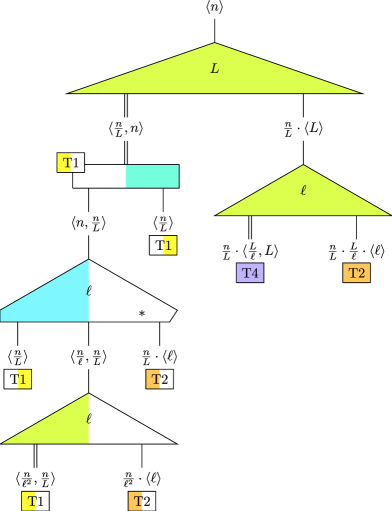
First, note that table-lookup variant T1 can deal with a multiset whose size and span are both bounded by some $N\in\mathbb{N}$ as easily as with a simple subset of $\{1,\ldots,N\}$. If a set $S$ of integers is of span $n$ and size $m$ and $\lambda\in\mathbb{N}$, then $g_{\lambda}(\mskip-3.0mu(S)\mskip-3.0mu)$ can be given span $\lceil\frac{n}{\lambda}\rceil+1$ and is of size $m$. As can be seen from Fig. 4, this implies that every CR1-node whose left and middle children are both T1-leaves can be replaced by a BR1-node with a T1-leaf as its left child and the former right child of the CR1-node as its right child. In other words, we can do away with an instance of the reduction BR2 and a T1-leaf. This applies to the inner node of maximal depth in Fig. 6 (and also in Fig. 5).

Second, a similar modification can be carried out at the right child $u$ of the root in Fig. 6. Begin by dissolving the reduction CR1 into its constituent parts, BR1 and BR2. Then the BR2-node can be seen to be in charge of answering queries about multisets whose span, $1+\frac{L}{\ell}$, is significantly smaller than their size, $L$. For such multisets we introduce another table-lookup variant:

T4.

If $S$ is a variable multiset of size at most $M$ consisting of integers in $\{1,\ldots,N\}$ for some given $N\in\mathbb{N}$, $S$ can be represented by the $N$-tuple $(\hbox{{rank\/}}_{S}(1),\ldots,\hbox{{rank\/}}_{S}(N))$ of integers in $\{0,\ldots,M\}$. Each of the $N$ integers can in turn be represented in $\lceil\log_{2}(M+1)\rceil$ bits. Since $2^{\lceil\log_{2}(M+1)\rceil}\leq 2M$, we can answer rank and select queries about a multiset stored in this way with a table of $O((2M)^{N+1}\log M)$ bits that can be computed in $O((2M)^{N+1})$ time.

We now replace the BR2-node and its children, a T3-leaf and a T2-leaf, by a T4-leaf with the parameters $N=1+L/\ell$ and $M=L$. For each of $O(\frac{n}{L})$ multisets, the T4-leaf must store $O(\frac{L}{\ell})$ integers, each of $O(\log L)$ bits, a total of $O({{n\log\log n}/{\log n}})$ bits. The size of the global table needed by the T4-leaf and the time to compute it can be seen to be negligible.

Third, in some cases where a reduction is used to answer rank and select queries, it may be possible to handle one of the two operations directly with table lookup. This speeds up the operation in question, but because the relevant subtree can be tuned to deal only with the other operation, additional benefits may accrue. To apply this observation most effectively, we also dissolve the combined reduction CR1 at the root in Fig. 6 into its constituent parts, BR1 and BR2. Since the new BR2-node $u$ is in charge of queries about a multiset of large size ($n$) but small span (approximately $\frac{n}{L}$), it can answer rank queries with table-lookup variant T1—the necessary table is of $O(\frac{n}{L}\log n)=O({{n\log\log n}/{\log n}})$ bits. As can be seen from Equation (4), this means that $u$ will issue only rank queries to its left child $v$ (the left child of the root in Fig. 6) and only select queries to its right child (the middle child of the root). The discussion in Subsection 4.2 then implies that $v$ will in turn issue only select queries to its left child and rank queries to its middle and right children, and this pattern repeats at $v$’s middle child.

We must still describe how to construct an index modified as above. Each change conceptually begins by replacing a CR1-node by a BR1-node and a BR2-node. Consider a BR1-node $u$ with parameter $\lambda$ whose input stream is a bit-vector representation of a set $S$ for which the alignment assumption holds. As described for CR1-nodes in Subsection 4.3, $u$ consumes its input in batches of $\lambda$ consecutive bits, counts the number $k$ of 1s in each batch, sums these counts in a variable $s$ that is initialized to $0$, and passes on every batch to its right child. Where the behavior of $u$ differs from that of CR1-nodes is in its communication with its left child. Informally, the multiset $g_{\lambda}(\mskip-3.0mu(S)\mskip-3.0mu)$ is represented by the prefix sums of its multiplicities. More precisely, $u$ transmits to its left child the value of its variable $s$ both before the processing of the first batch (when $s=0$) and after the processing of each batch (not just after batches that contain 1s).

Consider next a BR2-node $u$. By what was just described, $u$ receives a nondecreasing sequence of integers from its parent. When receiving the first integer, which is 0, it stores it in a variable $s$ and sends a 1 to its left child. For each subsequent integer $s^{\prime}$, $u$ does the following: If $s^{\prime}>s$, $u$ computes $k=s^{\prime}-s$, sends $k-1$ 0s followed by a 1 to its left child, sends a 1 to its right child, and sets $s:=s^{\prime}$. If $s^{\prime}=s$, $u$ just sends a 0 to its right child.

It can be seen that a BR1-node and a BR2-node, combined as in Fig. 2, together exhibit the behavior of a CR1-node whose left child is not a T3-node. On the other hand, if the left child of a BR1-node is a T1-leaf or a T4-leaf instead of a BR2-node, the leaf can easily construct its table, as described earlier in this subsection, from the stream that it receives.

A tuned rank-select index that incorporates the modifications discussed in this subsection is shown in Fig. 7. The notation $\langle\mbox{span},\mbox{size}\rangle$ is now used also to characterize the salient properties of multisets, but for a multiset the size may exceed the span. The operations rank and select were associated arbitrarily with the left and right halves, respectively, of (the graphical representation of) each node, and if a node handles only queries of one kind, only its corresponding half is shown colored (by a rainbow color or gray). The resulting savings, in terms of space, can be estimated from a comparison of Figs. 6 and 7 (note here that relieving a T2-leaf of the burden of answering either rank or select queries—but not both—does not reduce the number of bits that the leaf must store).

Figure 7: A tuned rank-select index with smaller tables and early completion of some queries.

The evaluation of rank queries in the tuned index follows a recipe that goes back to Jacobson [9, 10] and can hardly be improved upon: The client sequence $B$ is partitioned into superblocks, each of these in turn is partitioned into blocks, and to compute $\hbox{{rank\/}}_{B}(j)$ we locate the superblock and the simple block that contain the $j$th bit (call these the target superblock and block) and add the number of 1s before the target superblock (found in a first-level directory), the number of 1s in the target superblock but before the target block (found in a second-level directory), and the number of 1s in the target block until and including the $j$th bit of $B$, the latter quantity being computed with table-lookup variant T2.

References

- [1] D. Angluin and L. G. Valiant. Fast probabilistic algorithms for Hamiltonian circuits and matchings. J. Comput. Syst. Sci., 18(2):155–193, 1979.
- [2] David Clark. Compact Pat Trees. PhD thesis, University of Waterloo, 1997.
- [3] Peter Elias. Efficient storage and retrieval by content and address of static files. J. ACM, 21(2):246–260, 1974.
- [4] Robert M. Fano. On the number of bits required to implement an associative memory. Computation Structures Group Memo 61, MIT Project MAC, August 1971.
- [5] Alexander Golynski. Optimal lower bounds for rank and select indexes. Theor. Comput. Sci., 387(3):348–359, 2007.
- [6] Roberto Grossi, Ankur Gupta, and Jeffrey Scott Vitter. High-order entropy-compressed text indexes. In Proc. 14th Annual ACM–SIAM Symposium on Discrete Algorithms, pages 841–850. SIAM, 2003.
- [7] Torben Hagerup. Sorting and searching on the word RAM. In Proc. 15th Annual Symposium on Theoretical Aspects of Computer Science (STACS 1998), volume 1373 of LNCS, pages 366–398. Springer, 1998.
- [8] Torben Hagerup, Frank Kammer, and Moritz Laudahn. Space-efficient Euler partition and bipartite edge coloring. In Proc. 10th International Conference on Algorithms and Complexity (CIAC 2017), volume 10236 of LNCS, pages 322–333. Springer, 2017.
- [9] Guy Jacobson. Succinct static data structures. PhD thesis, Carnegie Mellon University, 1988.
- [10] Guy Jacobson. Space-efficient static trees and graphs. In Proc. 30th Annual IEEE Symposium on Foundations of Computer Science (FOCS 1989), pages 549–554. IEEE Computer Society, 1989.
- [11] Veli Mäkinen and Gonzalo Navarro. Rank and select revisited and extended. Theor. Comput. Sci., 387(3):332–347, 2007.
- [12] Mihai Pǎtraşcu. Succincter. In Proc. 49th Annual IEEE Symposium on Foundations of Computer Science (FOCS 2008), pages 305–313. IEEE Computer Society, 2008.
- [13] Rajeev Raman, Venkatesh Raman, and Srinivasa Rao Satti. Succinct indexable dictionaries with applications to encoding k-ary trees, prefix sums and multisets. ACM Trans. Algorithms, 3(4), 2007.