Adaptive PCA for Time-Varying Data

Abstract

In this paper, we present an online adaptive PCA algorithm that is able to compute the full dimensional eigenspace per new time-step of sequential data. The algorithm is based on a one-step update rule that considers all second order correlations between previous samples and the new time-step. Our algorithm has $\mathcal{O}\left(n\right)$ complexity per new time-step in its deterministic mode and $\mathcal{O}\left(1\right)$ complexity per new time-step in its stochastic mode. We test our algorithm on a number of time-varying datasets of different physical phenomena. Explained variance curves indicate that our technique provides an excellent approximation to the original eigenspace computed using standard PCA in batch mode. In addition, our experiments show that the stochastic mode, despite its much lower computational complexity, converges to the same eigenspace computed using the deterministic mode.

1 Introduction

Principal Component Analysis (PCA) is one of the most important machine learning techniques for many reasons. Firstly, it is the only unsupervised learning algorithm that is theoretically proven to capture the maximal variability (information) of the input data given a fixed-size low-dimensional space. Another main reason is that it directly deals with the eigenspace of the problem on hand. In the real world, an endless amount of problems and physical phenomena can be modelled by eigenvalue equations. One important example is the Dirac equation which assumes that all variables of a physical object (speed, acceleration, etc) obey an eigenvalue problem [30]. In quantum physics, the quantum states that an electron in an atom can take (labeled as 1S, 2S, 2P etc) are actually time-dependent eigenfunctions which are called “quantum eigenstates” [33].

Despite the elegance of PCA, it has not been widely used until the last four decades. One reason for this is that, in its basic form, it has a quadratic space and time complexity which requires large memory and processing speed. Nowadays machines are shown to be more capable of handling such complexity thanks to larger available memory and faster CPU and GPU (Graphics Processing Unit) capabilities. However, for a wide range of problems where the dimensionality of the data is massive (due to the size and number of samples), extracting the principal components in the standard way becomes infeasible. Many algorithms have been developed to find the most significant principal components with linear complexity dependence on data size. However most of these approaches are stochastic and are limited to extracting a certain number of eigenvectors (principal components).

In this paper, we consider time-dependent systems that require regular monitoring and analysis for each new time-step. This is particularly important, for instance, in equilibria and stability analysis of the system. In many physical phenomena, such as the electron eigenstates example mentioned above, the time-dependent behavior of the significant eigenvectors converges to an equilibrium eigenstate. We propose an adaptive PCA algorithm that is able to capture all eigenvectors of the data and has $\mathcal{O}\left(n\right)$ complexity per new time-step in its deterministic mode and $\mathcal{O}\left(1\right)$ complexity per new time-step in its stochastic mode, where $n$ is the number of previous time-steps. We test this algorithm on six time-varying datasets of different physical phenomena. We compare the performance of our algorithm with the standard PCA applied in batch-mode.

2 Background and Related Work

In the literature, there are two main directions that PCA research has taken. The first is that concerning applications which employ PCA for solving real-world problems and the second is that in the direction of PCA-optimization which is concerned with the optimization of the computational complexity of PCA. The link between the two directions is not clear since most studies in the application direction assume a pre-computed eigenspace and focus mainly on the distribution of test data in that eigenspace. On the other hand, in the optimization direction, the target use-case is not obvious. In addition, most of the optimization-direction algorithms are of a stochastic nature and are usually tested on rather simple datasets or data where a global eigenspase can be easily derived. In such a case, one can always consider a pre-computed eigenspace no matter what computational complexity was required for finding it. In fact, many online datasets provide a list of the most significant eigenvectors of the studied samples.

With regard to the applications research, the use of PCA has been well reported in the fields such as Computer Vision and Computer Graphics. For instance, in facial recognition, Kirby and Sirovich [17] proposed PCA as a holistic representation of the human face in 2D images by extracting few orthogonal dimensions which form the face-space and were called eigenfaces [36]. Gong et al. [13] were the first to find the relationship between the distribution of samples in the eigenspace, which were called manifolds, and the actual pose in an image of a human face. The use of PCA was extended using Reproducing Kernel Hilbert Spaces which non-linearly map the face-space to a much higher dimensional space (Hilbert space)  [37]. Knittel and Paris [18] employed a PCA-based technique to find initial seeds for vector quantization in image compression. There are a number of previous reported uses of PCA-related methods in the computer graphics and visualization literature. For instance, Nishino et al. [24] proposed a method, called Eigen-texture, which creates a 3D image from a sample of range images using PCA. They found that partitioning samples into smaller cell-images improved the rendering of surface-based 3D data. Grabner et al. [14] proposed a hardware accelerated technique that uses the multiple eigenspaces method [20] for image-based reconstruction of a 3D polygon mesh model. Liu et al. [21] employed PCA for dynamic projections in the visualization of multivariate data. Broersen et al. [7] discussed the use of PCA techniques in the generation of transfer functions, which are used to assign optical properties such as color and opacity to attributes in volume data. Takemoto et al. [34] used PCA for feature space reduction to support transfer funtion design and exploration of volumetric microscopy data. Fout and Ma [9] presented a volume compression method based on transform coding using the Karhunen-Loève Transform (KLT), which is closely related to PCA.

In the PCA-optimization research, the power iteration remains one of the most popular techniques for finding the top $p$ eigenvectors [12]. In the recent leterature, Shamir proposed a stochastic PCA algorithm that is proven to converge faster than the power iteration method [31]. Both techniques have a lower bound complexity of $\mathcal{O}\left(n\log\left(\frac{1}{\epsilon}\right)\right)$ where $\epsilon$ is the precision of convergence. In addition, both techniques were experimentally tested to extract only a limited number of significant eigenvectors. Arora and De Sa et al. [2, 3, 8] proposed stochastic techniques that are based on the gradient-descent learning rule. The slow convergence rate of the gradient-descent rule is one main limitation of these techniques. Many algorithms were developed to find eigenvectors incrementally per new number of time-steps. Such techniques are referred to as incremental PCA algorithms. The update schemes proposed by Krasulina [19] and Oja [25, 26] are the most popular incremental PCA techniques. Given a new time-step $x_{n+1}$ and a significant eigenvector $v$ for previous samples, the general update rule according to Oja’s method is

$$v^{i+1}=v^{i}+\alpha\left\langle x_{n+1},v^{i}\right\rangle x_{n+1};\;v^{i+1}=\frac{v^{i+1}}{\left\|v^{i+1}\right\|},$$

where $\alpha$ is the learning rate. This process will keep updating until converging to a stable state. The speed of convergence of this technique is a matter of ongoing research. Balsubramani et al. [4] found that speed of convergence depends on the learning rate $\alpha$. Another problem with this technique (as we will find later in this study) is that it does not consider change in weightings of previous time-steps. Mitiagkas et al. proposed an incremental PCA algorithm for streaming data with computational complexity of $\mathcal{O}\left(n\log\left(n\right)\right)$ [23].

One important point to highlight is that most studies in both directions focus mainly on the most significant eigenvectors with little attention paid to the least significant ones. In fact, finding such eigenvectors was shown to play a key role in detecting outliers and non-belonging samples since they are perpendicular to the best fitting hyperplane. Jollife [16] pointed out in his book that the principal components corresponding to the smallest eigenvalues (variances) are not “unstructured left -overs” after extracting the higher PCs and that they can be useful in detecting outliers. The first use of the smallest PC in the literature was done by Gnanadesikan and Wilk 1969 [11]. Based on this work, Gnanadesikan [10] stated that “with p-dimensional data, the projection onto the smallest principal component would be relevant for studying the deviation of an observation from a hyperplane of closest fit”. More recently, Izenman and Shen used the smallest kernel principal components for outlier detection as a generalization of the linear case [15]. Alakkari et al. found that the least significant eigenface can be used as a basis for discriminating between face and non-face images [1]. In Partial Differential Equations, many systems are solved by seeking a hyperplane that is constituted of the entire solution. This is known as the method of characteristics.

3 Concepts

The standard approach to PCA is as follows. Given data samples $X=[x_{1}\,x_{2}\cdots x_{n}]\in\mathbb{R}^{d\times n}$, where each sample is in column vector format, the covariance matrix is defined as

$$C=\frac{1}{n-1}\sum_{i=1}^{n}\left(x_{i}-\bar{x}\right)\left(x_{i}-\bar{x}\right)^{T},$$ (1)

where $\bar{x}$ is the sample mean. In the sequel of this paper, we will assume that all samples are centered and hence there is no need to subtract the sample mean explicitly. After computing the covariance matrix, we can find the optimal low-dimensional bases that cover most variability in samples by extracting the significant eigenvectors of the covariance matrix $C$. Eigenvectors are extracted by solving the following eigenvalue equation

$$\left(C-\lambda I\right)v=0;\,v^{T}v=1,$$ (2)

where $v\in\mathbb{R}^{d}$ is the eigenvector and $\lambda$ is its corresponding eigenvalue. Eigenvalues describe the variance maintained by the corresponding eigenvectors. Hence, we are interested in the subset of eigenvectors that have the highest eigenvalues $V=[v_{1}\,v_{2}\cdots v_{p}];\,p\ll n$. Then we encode a given sample $x$ using its $p$-dimensional projection values (referred to as scores) as follows

$$W=V^{T}x.$$ (3)

We can then reconstruct the sample as follows

$$x_{reconstructed}=VW.$$ (4)

One advantage of PCA is the low computational complexity when it comes to encoding and reconstructing samples.

Duality in PCA

Since in the case of $n\ll d$, $C$ will be of rank $n-1$ and hence there are only $n-1$ eigenvectors that can be extracted from Eq. (2) and since $C$ is of size $d\times d$, solving Eq. (2) becomes computationally expensive. We can find such eigenvectors from the dual eigenspace by computing the $n\times n$ matrix $X^{T}X$ and then solving the eigenvalue problem

$$\left(X^{T}X-(n-1)\lambda I\right)v_{dual}=0$$ (5)

$$\Rightarrow X^{T}Xv_{dual}=(n-1)\lambda v_{dual};\,v_{dual}^{T}v_{dual}=1.$$ (6)

Here, for simplicity, we assumed that the sample mean of $X$ is the zero vector. After extracting the dual eigenvectors, one can note that by multiplying each side of Eq. (6) by $X$, we have

$$XX^{T}Xv_{dual}=(n-1)\lambda Xv_{dual}$$

$$\Rightarrow\frac{1}{n-1}XX^{T}\left(Xv_{dual}\right)=\lambda\left(Xv_{dual}\right)$$

$$\Rightarrow C\left(Xv_{dual}\right)=\lambda\left(Xv_{dual}\right)$$

$$\Rightarrow\left(C-\lambda I\right)\left(Xv_{dual}\right)=0$$

which implies that

$$v=Xv_{dual}.$$ (7)

Thus, when $n\ll d$, we only need to extract the dual eigenvectors using Eq. (6) and then compute the real eigenvectors using Eq. (7). Only the first few eigenvectors $V_{p}=[v_{1}\>v_{2}\ldots v_{p}],\>p\ll n\ll d$ will be chosen to represent the eigenspace, those with larger eigenvalues.

4 Adaptive PCA Algorithm

The main premise of our algorithm is based on the fact that an eigenvector is actually a weighted sum of the input samples. We can show that by rewriting Eq. (2) as follows

$$\left(\frac{1}{n-1}\sum_{i=1}^{n}x_{i}x_{i}^{T}-\lambda I\right)v=0$$

$$\Rightarrow\frac{1}{n-1}\sum_{i=1}^{n}x_{i}x_{i}^{T}v-\lambda v=0$$

$$\Rightarrow\frac{1}{n-1}\sum_{i=1}^{n}x_{i}\left\langle x_{i},v\right\rangle-\lambda v=0$$

$$\Rightarrow v=\frac{1}{\lambda\left(n-1\right)}\sum_{i=1}^{n}\left\langle x_{i},v\right\rangle x_{i}.$$

A first guess for an update formula given new time-step $x_{n+1}$ would be

$$v^{t+1}=v^{t}+\left\langle x_{n+1},v^{t}\right\rangle x_{n+1};\;v^{t+1}=\frac{v^{t+1}}{\left\|v^{t+1}\right\|}.$$

This is similar to Oja’s update scheme mentioned in the background section. The problem with this formula is that it assumes the weightings of previous samples are fixed. As the eigenvector is updated for each new time-step, the weights of previous samples should also be adjusted according to their projections on the updated eigenvector. The change in weights will be proportional to the correlations between previous samples and the new time-step. In our algorithm we used the following update rule

$$v^{t+1} =v^{t}+\left(\sum_{j=1}^{n}\left\langle v^{t},x_{j}\right\rangle\left\langle x_{j},x_{n+1}\right\rangle^{2}x_{j}\right)+\left\langle v^{t},x_{n+1}\right\rangle\left(\sum_{j=1}^{n+1}\left\langle x_{j},x_{n+1}\right\rangle\right)^{2}x_{n+1}$$

$$=v^{t}+\left(\sum_{j=1}^{n}\left\langle v^{t},x_{j}\right\rangle\left\langle x_{j},x_{n+1}\right\rangle^{2}x_{j}\right)$$

$$\;\;\;\;\;\;\;\;+\left\langle v^{t},x_{n+1}\right\rangle\left(\sum_{j=1}^{n+1}\sum_{i=1}^{n+1}\left\langle x_{j},x_{n+1}\right\rangle\left\langle x_{i},x_{n+1}\right\rangle\right)x_{n+1};\;v^{t+1}=\frac{v^{t+1}}{\left\|v^{t+1}\right\|}.$$

Unlike Oja’s method, this is an online scheme that adapts weightings of all previous samples based on the squared dot product with the new time-step. In addition, the new time-step is weighted based on the sum of all second order dot products $\left\{\left\langle x_{i},x_{n+1}\right\rangle.\left\langle x_{j},x_{n+1}\right\rangle\right\}_{i,j=1}^{n+1}$ multiplied by new time-step’s score $\left\langle v^{t},x_{n+1}\right\rangle$. Since for each eigenvector, we are computing the correlations (dot products) between the new time-step $x_{n+1}$ and all $n$ previous samples and considering that scores (weights) of previous samples $\left\{\left\langle v^{t},x_{j}\right\rangle\right\}_{j=1}^{n}$ are computed in the previous iteration, this requires a time complexity of $\mathcal{O}\left(n\right)$ dot products per eigenvector per new time-step.

The full pseudo-code of our algorithm is shown in Algorithm 1. There are two parameters used in our algorithm: $space\_limit$ which specifies the maximal number of significant eigenvectors to compute and $processing\_limit$ which specifies the maximal number of dot products to compute per new time-step per eigenvector. As we mentioned earlier, our algorithm is capable of finding all eigenvectors of the data. In order to compute the full dimensional eigenspace deterministically, we set $space\_limit=\min(d,n)$ and $processing\_limit\gg n$ where $d$ is the total number of dimensions per sample and $n$ is the current number of samples. In its full-dimensional mode, our algorithm starts with two time-steps with $\frac{x_{2}-x_{1}}{\left\|x_{2}-x_{1}\right\|}$ as the initial eigenvector and ends with the full-dimensional eigenspace of the data. Line 1 of the algorithm includes the general update rule. Line 1 is used particularly for the limited processing mode (stochastic mode) to stress the shared information learned by $v^{t}$ and $v^{t+1}$. Line 1 performs a Gram-Schmidt process to ensure that following update terms will be orthogonal to updated eigenvector. After finishing the loop, $\tilde{X}$ will constitute the $n$th eigenvector since it will be perpendicular to all $n-1$ updated components.

1

2for each new time-step $x_{n+1}$ do

3       $X=\left[X,\;x_{n+1}\right]$;

4       $\tilde{X}=X$;

5       if $n>processing\_limit$ then

6             $indices=\text{rand}\left(n,processing\_limit\right)$;

7            

8      else

9             $indices=1:n$;

10            

11       end if

12      

13      for $i=1:\left(\min\left(n,space\_limit\right)-1\right)$ do

14             $\tilde{v}=v_{i}+\left(\sum_{j=indices}\left\langle v_{i},\tilde{x}_{j}\right\rangle\left\langle\tilde{x}_{j},\tilde{x}_{n+1}\right\rangle^{2}\tilde{x}_{j}\right)+\left\langle v_{i},\tilde{x}_{n+1}\right\rangle\left(\left(\sum_{j=indices}\left\langle\tilde{x}_{j},\tilde{x}_{n+1}\right\rangle\right)+\left\langle\tilde{x}_{n+1},\tilde{x}_{n+1}\right\rangle\right)^{2}\tilde{x}_{n+1}$;

15             $v_{i}=\tilde{v}+\left\langle\tilde{v},v_{i}\right\rangle v_{i}$;

16             $v_{i}=\frac{v_{i}}{\left\|v_{i}\right\|}$;

17             $\tilde{X}_{indices\cup\left\{n+1\right\}}=\tilde{X}_{indices\cup\left\{n+1\right\}}-v_{i}\left(v_{i}^{T}\tilde{X}_{indices\cup\left\{n+1\right\}}\right)$;

18            

19       end for

20      $v_{\min\left(n,space\_limit\right)}=\sum_{j=indices\cup\left\{n+1\right\}}\tilde{x}_{j}$;

21       $n=n+1$;

22      

23 end for

Algorithm 1 Adaptive PCA

4.1 Limited-Dimensional Adaptive PCA

In the limited dimensional mode of our algorithm, we set a maximal number of eigenvectors to update/compute per new time-step using the space_limit parameter. Since this parameter value is constant throughout the execution of our algorithm, this will bound the time complexity to $\mathcal{O}\left(space\_limit\times n\right)=\mathcal{O}\left(n\right)$ dot products per new time-step.

4.2 Limited-Dimensional Adaptive PCA in Stochastic Mode

In the stochastic mode, we specify a maximal number of dot products to be computed per new time-step per eigenvector. This happens when $n>processing\_limit$. In this case, we choose $processing\_limit$ uniformly distributed random samples to compute their dot products with the new time-step. This will further bound the time complexity to $\mathcal{O}\left(space\_limit\times processing\_limit\right)=\mathcal{O}\left(1\right)$ dot products per new time-step. Considering that our algorithm does not require the computation of the covariance matrix, the full time complexity of PCA in the stochastic mode will be $\mathcal{O}\left(n\right)$ dot products (after processing all time-steps of the input data).

5 Experimental Results

We applied our algorithm on six time-varying datasets of different physical phenomena. The first dataset studies the stages of a supernova during a period of less than one second after a star’s core collapses [6]. The second dataset studies the fluid dynamics in turbulent vortex in a 3D area of the fluid [32]. The third dataset shows the evolution of a splash caused after a drop impacts on a liquid surface [35]. The fourth dataset was generated to analyze the chaotic path of a drop of silicone oil bouncing on the surface of a vibrating bath of the same material [27]. The fifth experimental data shows the unusual behaviour of some particles self-organized into spirals after rotational fluid flow [29]. Finally, the sixth dataset shows the behaviour of nitrogen bubbles cascading down the side of a glass of Guinness (dark beer), which has been well-investigated in a number of papers [5, 28]. Table 1 summarizes the properties of each dataset. The first two datasets are in the form a 3D scalar field (i.e. voxels datasets). The remaining four datasets are in video format and were adapted from original sources by converting to greyscale video frames and cropping these frames to a segment of interest (the most highly varying part of the video sequence). The adapted datasets can be obtained by emailing the authors.

Table 1: Summary of the datasets used in our experiments.

dataset/experiment name	data type	time-step resolution	number of time-steps
Supernova	3D volumes	$432^{3}$ voxels	60
Turbulent Vortex	3D volumes	$128^{3}$ voxels	100
Droplet Impact on Liquid Surface	grayscale video	$240\times 312$ pixels	100
Bouncing Silicone Drop	grayscale video	$300\times 640$ pixels	300
Self Organized Particles	grayscale video	$54\times 152$ pixels	650
Guinness Cascade	grayscale video	$271\times 131$ pixels	1,100

We compare the performance of our algorithm with standard PCA in terms of explained variance curves. The standard PCA results are generated using the pcacov function in MATLAB [22]. Since we are dealing with cases where $n\ll d$, it is typical to use the dual covariance matrix $X^{T}X$ for standard PCA. For the adaptive PCA, we incrementally update the eigenvectors until reaching the last time-step as in Algorithm 1.

Figure 1: Explained variance curves of standard PCA and full-dimesional adaptive PCA for each dataset.

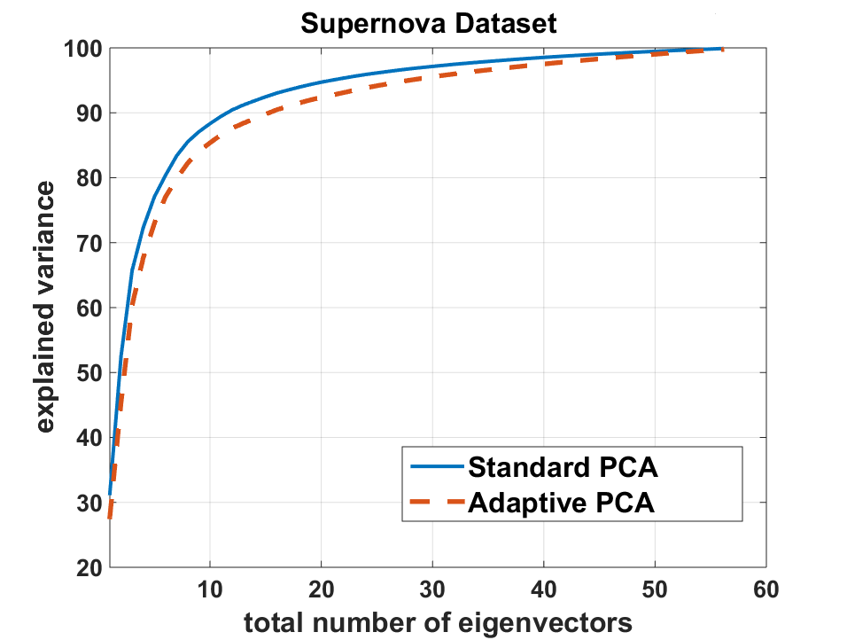
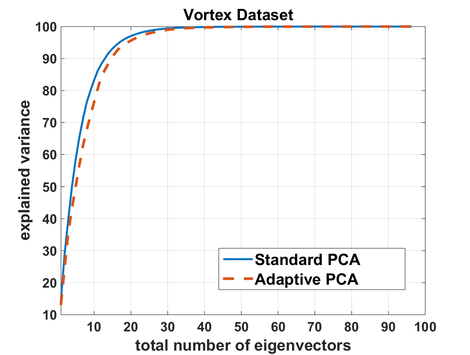
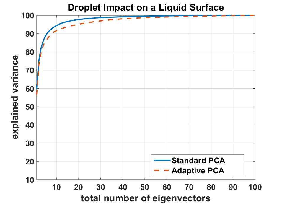
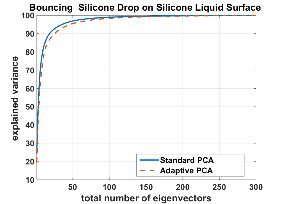
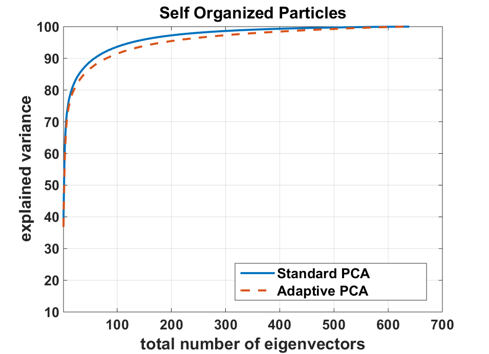
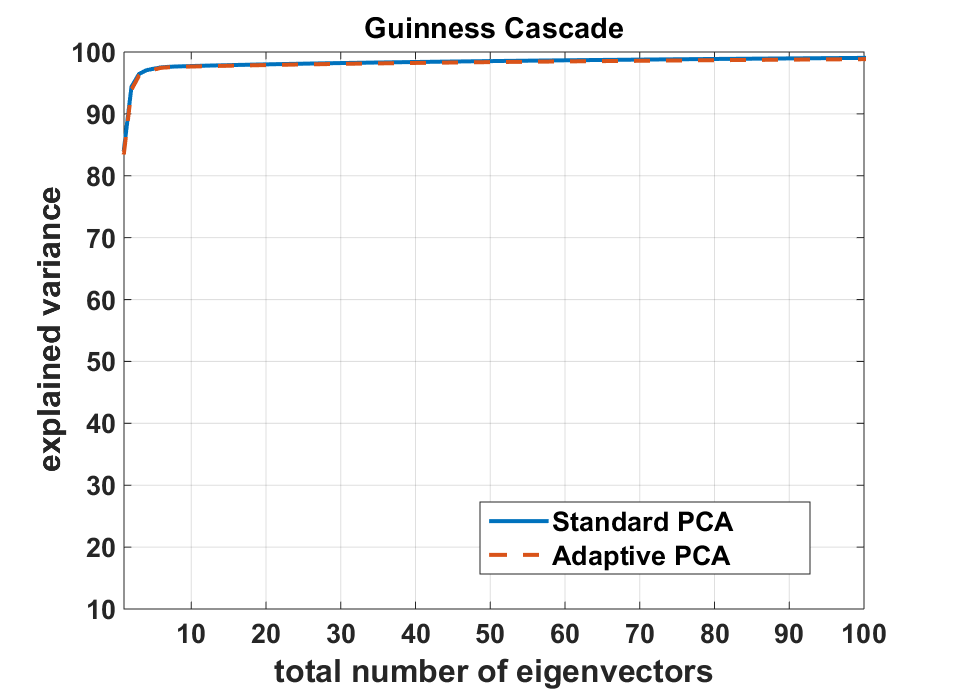
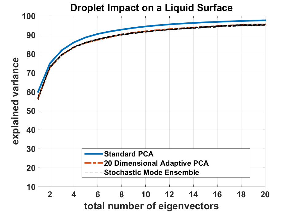
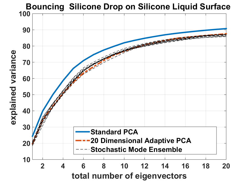
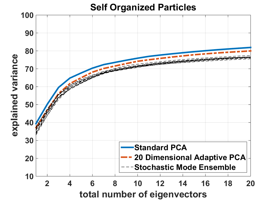
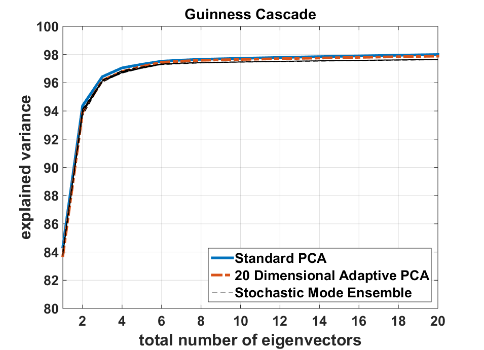
We first do a comparison between the full-dimensional eigenspace computed using each technique. This is to stress the capability of our approach of finding all eigenvectors of the given datasets. Figure 1 shows the explained variance curves for each dataset. It is very clear that our algorithm provides an excellent approximation to the original full-dimensional eigenspace. For all datasets, the gap between the two curves does not exceed $2\%$. It is also interesting to note how well both techniques were able to learn the guinness cascade phenomenon, where $98\%$ of the variability was covered by only the first 20 eigenvectors.

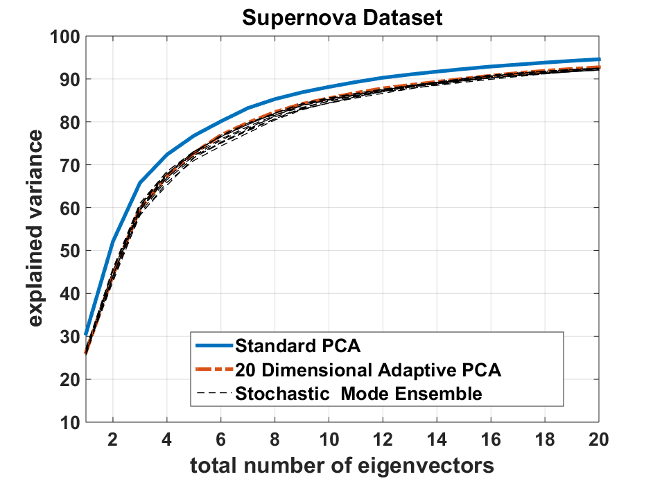
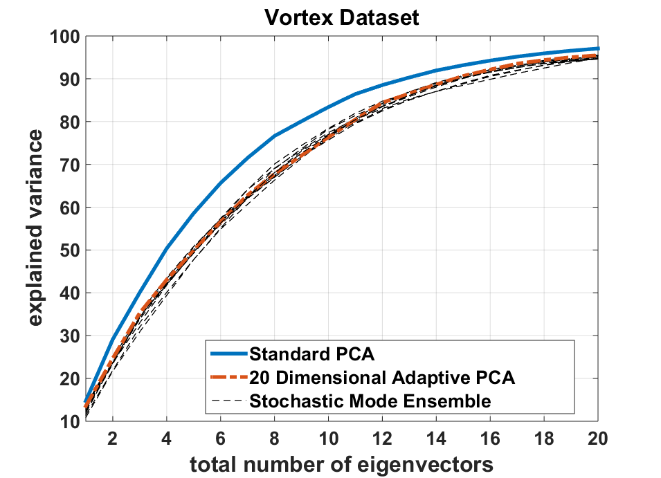
Next we compute the limited-dimensional eigenspace for each dataset mainly to compare performance between deterministic and stochastic modes of our algorithm. Figure 2 shows the performance of the 20-dimensional adaptive PCA. To test the stochastic mode performance, we applied 10 runs of our algorithm where in each run we set $processing\_limit$ to 40. With much lower number of computations, the stochastic runs achieve almost the same performance as the deterministic mode. The only difference one can note is in the Self Organized Particles experiment where the stochastic runs provide mean explained variance of $77\%$ while the deterministic mode covers $80\%$ of variability.

Figure 2: Explained variance curves of standard PCA and 20-dimensional adaptive PCA in both deterministic and stochastic modes for each dataset.

6 Conclusion

In this paper, we presented a deterministic scheme that finds the eigenspace of sequential data incrementally with linear time complexity growth. Our model is a generalization of Oja’s method with the following two main advantages. In our approach, the eigenvectors are updated in an online manner (one-step update per eigenvector) unlike Oja’s method which is applied in an iterative manner per eigenvector. Secondly, our model considers all previous samples in its update formula whereas Oja’s method considers only the most recent time-step in its update rule. Since our algorithm considers all second order correlations between samples, this provides an intensive learning scheme that better resembles the quadratic nature of standard PCA. In the limited-computations mode of our algorithm (stochastic mode), the eigenvectors are adapted according to the pattern learned from limited population ensembles. Our experiments have shown that the stochastic mode provides the same performance as the deterministic mode with much lower number of computations. Our technique serves as a robust modeling tool for complex time-dependent systems that decomposes the systems temporal behaviour using orthogonal time-dependent functions which correspond to the dual eigenspace. This can be expressed as follows

$$\vec{S}_{t}=\sum_{i=1}^{p}v_{i}f_{i}\left(t\right)=\sum_{i=1}^{p}v_{i}\left(v_{i}^{T}x_{t}\right).$$

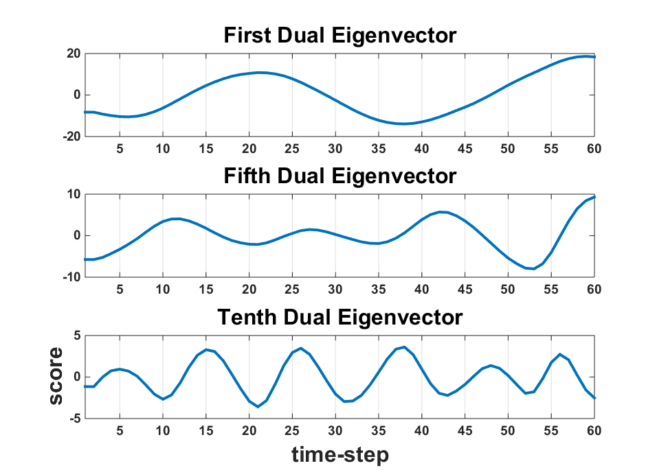
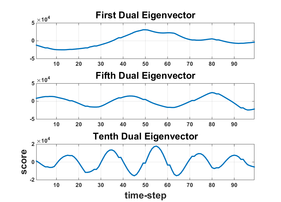
Figures 3 shows the time-dependent functions of the first, fifth and tenth eigenvectors for the Supernova and Vortex datasets. One can note that the higher significance eigenfunctions have lower frequency with higher amplitude. By interpolating these functions, we can analyze the system behavior in continuous time. In terms of future work, it would be interesting to know the performance of our algorithm using different distributions of previous samples in the stochastic mode. In many systems, the recent samples have higher priority than older ones, such as in CCTV surveillance applications where the records are saved for a limited period of time.

Figure 3: Three time-dependent eigenvectors for Supernova (left) and Vortex (right) datasets.

Acknowledgments

This research has been conducted with the financial support of Science Foundation Ireland (SFI) under Grant Number 13/IA/1895.

References

- [1] S. Alakkari, E. Gath, and J. J. Collins. An investigation into the use of subspace methods for face detection. In Neural Networks (IJCNN), 2015 International Joint Conference on, pages 1–7. IEEE, 2015.
- [2] R. Arora, A. Cotter, K. Livescu, and N. Srebro. Stochastic optimization for PCA and PLS. In Communication, Control, and Computing (Allerton), 2012 50th Annual Allerton Conference on, pages 861–868. IEEE, 2012.
- [3] R. Arora, A. Cotter, and N. Srebro. Stochastic optimization of PCA with capped MSG. In Advances in Neural Information Processing Systems, pages 1815–1823, 2013.
- [4] A. Balsubramani, S. Dasgupta, and Y. Freund. The fast convergence of incremental PCA. In Advances in Neural Information Processing Systems, pages 3174–3182, 2013.
- [5] E. Benilov, C. Cummins, and W. Lee. Why do bubbles in guinness sink? American Journal of Physics, 81(2):88–91, 2013.
- [6] J. Blondin. Supernova dataset. http://vis.cs.ucdavis.edu/VisFiles/pages/supernova.php.
- [7] A. Broersen, R. van Liere, and R. M. Heeren. Comparing three PCA-based methods for the visaulization of imaging spectroscopy data. In Proceedings of the Fifth IASTED International Conference on Visualization, Imaging and Image Processing, pages 540–545, September 2005.
- [8] C. De Sa, K. Olukotun, and C. Ré. Global convergence of stochastic gradient descent for some non-convex matrix problems. arXiv preprint arXiv:1411.1134, 2014.
- [9] N. Fout and K. L. Ma. Transform coding for hardware-accelerated volume rendering. IEEE Transactions on Visualization and Computer Graphics, 13(6):1600–1607, Nov 2007.
- [10] R. Gnanadesikan and J. R. Kettenring. Robust estimates, residuals, and outlier detection with multiresponse data. Biometrics, pages 81–124, 1972.
- [11] R. Gnanadesikan and M. Wilk. Data analytic methods in multivariate statistical analysis. Multivariate analysis, 2:593–638, 1969.
- [12] G. H. Golub and C. F. Van Loan. Matrix computations, volume 3. JHU Press, 2012.
- [13] S. Gong, S. McKenna, and J. J. Collins. An investigation into face pose distributions. In Automatic Face and Gesture Recognition, 1996., Proceedings of the Second International Conference on, pages 265–270. IEEE, 1996.
- [14] M. Grabner, H. Bischof, C. Zach, and A. Ferko. Multiple eigenspaces for hardware accelerated image based rendering. in Proceedings of ÖAGM, pages 111–118, 2003.
- [15] A. J. Izenman and Y. Shen. Outlier detection using the smallest kernel principal components. Astro Temple Edu, pdf report, 2009.
- [16] I. Jolliffe. Principal component analysis. Wiley Online Library, 2002.
- [17] M. Kirby and L. Sirovich. Application of the karhunen-loeve procedure for the characterization of human faces. Pattern Analysis and Machine Intelligence, IEEE Transactions on, 12(1):103–108, 1990.
- [18] G. Knittel and R. Parys. PCA-based seeding for improved vector quantization. In Proceedings of the First International Conference on Computer Imaging Theory and Applications (VISIGRAPP 2009), pages 96–99, 2009.
- [19] T. Krasulina. A method of stochastic approximation for the determination of the least eigenvalue of a symmetric matrix. Zhurnal Vychislitel’noi Matematiki i Matematicheskoi Fiziki, 9(6):1383–1387, 1969.
- [20] A. Leonardis and H. Bischof. Multiple eigenspaces by mdl. In Proceedings 15th International Conference on Pattern Recognition. ICPR-2000, volume 1, pages 233–237 vol.1, 2000.
- [21] S. Liu, B. Wang, J. J. Thiagarajan, P. T. Bremer, and V. Pascucci. Multivariate volume visualization through dynamic projections. In 2014 IEEE 4th Symposium on Large Data Analysis and Visualization (LDAV), pages 35–42, Nov 2014.
- [22] The Mathworks, Inc., Natick, Massachusetts. MATLAB and Statistics Toolbox Release 2017a, 2017.
- [23] I. Mitliagkas, C. Caramanis, and P. Jain. Memory limited, streaming pca. In Advances in Neural Information Processing Systems, pages 2886–2894, 2013.
- [24] K. Nishino, Y. Sato, and K. Ikeuchi. Eigen-texture method: Appearance compression based on 3D model. In Computer Vision and Pattern Recognition, 1999. IEEE Computer Society Conference on., volume 1. IEEE, 1999.
- [25] E. Oja. Simplified neuron model as a principal component analyzer. Journal of mathematical biology, 15(3):267–273, 1982.
- [26] E. OJE. Subspace methods of pattern recognition. In Pattern recognition and image processing series, volume 6. Research Studies Press, 1983.
- [27] S. Perrard, E. Fort, and Y. Couder. Wave-based turing machine: Time reversal and information erasing. Physical review letters, 117(9):094502, 2016.
- [28] O. Power, W. Lee, A. Fowler, P. Dellar, L. Schwartz, S. Lukaschuk, G. Lessells, A. Hegarty, M. O’Sullivan, and Y. Liu. The initiation of guinness. 2009.
- [29] D. Pushkin, D. Melnikov, and V. Shevtsova. Ordering of small particles in one-dimensional coherent structures by time-periodic flows. Physical review letters, 106(23):234501, 2011.
- [30] C. Rovelli. Quantum gravity. Cambridge university press, 2007.
- [31] O. Shamir. A stochastic pca and svd algorithm with an exponential convergence rate. In ICML, pages 144–152, 2015.
- [32] D. Silver. Turbulent vortex dataset. http://www.cs.ucdavis.edu/~ma/ITR. Available from the Time-varying data repository at UCDavis.
- [33] W. F. Smith. Waves and oscillations: a prelude to quantum mechanics. Oxford University Press, 2010.
- [34] S. Takemoto, M. Nakao, T. Sato, T. Sugiura, K. Minato, and T. Matsuda. Interactive volume visualization of microscopic images using feature space reduction. BME, 51:U–6–U–6, 2013.
- [35] M.-J. Thoraval, K. Takehara, T. G. Etoh, S. Popinet, P. Ray, C. Josserand, S. Zaleski, and S. T. Thoroddsen. von kármán vortex street within an impacting drop. Physical review letters, 108(26):264506, 2012.
- [36] M. Turk and A. Pentland. Eigenfaces for recognition. Journal of cognitive neuroscience, 3(1):71–86, 1991.
- [37] M. H. Yang. Kernel eigenfaces vs. kernel fisherfaces: Face recognition using kernel methods. In Proceedings of Fifth IEEE International Conference on Automatic Face Gesture Recognition, pages 215–220, May 2002.