Deterministic physical systems under uncertain initial conditions: the case of maximum entropy applied to projectile motion

Abstract

The kinematics and dynamics of deterministic physical systems have been a foundation of our understanding of the world since Galileo and Newton. For real systems, however, uncertainty is largely present via external forces such as friction or lack of precise knowledge about the initial conditions of the system. In this work we focus in the latter case and describe the use of inference methodologies in solving the statistical properties of classical systems subject to uncertain initial conditions. In particular we describe the application of the formalism of Maximum Entropy (MaxEnt) inference to the problem of projectile motion given information about the average horizontal range over many realizations. By using MaxEnt we can invert the problem and use the provided information on the average range to reduce the original uncertainty in the initial conditions, while also achieving additional insights based on the shape of the posterior probabilities for the initial conditions probabilities and the projectile path distribution itself. The wide applicability of this procedure, as well as its ease of use, reveals a useful tool by which to revisit a large number of physics problems, from classrooms to frontier research.

1 Introduction

Classical mechanical systems are completely deterministic, following well-established equations of motion such as Newton’s second law or Hamilton equations. However, uncertainty still is introduced in the lack of control of the initial conditions of a mechanical system. Usually mechanical systems are chaotic, that is, highly sensitive to these initial conditions, with the corresponding loss of predictability. Given a certain statistical distribution of initial conditions, the result is of course a (non-trivial) statistical distribution of outcomes, obtained by propagating the system forwards in time according to the equations of motion. This suggests the opposite situation: given statistical properties of the outcomes of a classical system, can we obtain some information about the initial conditions that produced these outcomes? This is an inverse problem from the point of view of probability theory, which can in principle be addressed using Bayes’ theorem [1] and/or information theoretical methods [2].

Since the time of Galileo Galilei, projectile motion has been a widely studied phenomenon from a large set of different approaches. These range from including the presence of a resisting medium [3], to highly accurate analytical functions [4]. This particular motion presents an almost endless list of uses in different technological areas, such as ballistics [5, 6, 7, 8], sports [9, 10], rockets among others [11, 12]. In spite of the large body of information on projectile motion we are not aware of previous work where it is treated as an inverse problem in which information at later times is known and we infer the initial conditions.

In this work we propose and solve the problem of a large number of realizations of projectile motion with known average horizontal range $\bar{R}$, where we infer the most unbiased probability distribution of initial angle $\theta_{0}$ and speed $v_{0}$. This is achieved by the use of the Maximum Entropy principle (MaxEnt).

Our application to projectile motion is only a guide to the proposed procedure, and its choice is based fundamentally in strengthening statistical methods in students. By understanding the theoretical foundations that allow the solution of this kind of problems, students will be able to diversify their applicability to many other problems known in physics.

2 The principle of Maximum Entropy

The principle of maximum entropy [13] (MaxEnt for short), proposed by Edwin T. Jaynes in 1957, is extensively used as a general tool of probabilistic inference [14] applicable to numerical data analysis, image reconstruction, and inverse problems in general. In its modern formulation, MaxEnt establishes than the most unbiased probability distribution $P$ given some state of knowledge $I$ is the one that maximizes the Shannon-Jaynes entropy $S[P]$ (known also as relative entropy or the negative of the Kullback-Leibler divergence), given by [15]

$$\centering S(I_{0}\rightarrow I)=-\int d\bm{x}P(\bm{x}|I)\ln\frac{P(\bm{x}|I)}{P(\bm{x}|I_{0})},\@add@centering$$ (1)

while being consistent with said knowledge. Here $\bm{x}=(x_{1},\ldots,x_{N})$ is the $N$-component vector of continuous degrees of freedom of the system and $P(\bm{x}|I_{0})$ represents a prior probability distribution, used as a starting point for the inference.

By maximizing $S(I_{0}\rightarrow I)$ in Eq. 1, we obtain the probabilistic model that contains the least amount of information (i.e. the least biased) while reproducing the features one demands of it. Consider a constraint on the known expectation $f_{0}$ of a function $f(\bm{x})$ (this knowledge is represented by $I$). According to MaxEnt, the most unbiased model is given by maximizing $S$ in Eq. 1 with the constraint $\left<f(\bm{x})\right>=f_{0}$. The constrained maximization problem is usually implemented by means of a Lagrange multiplier $\lambda$, which leads to the well-known maximum entropy model,

$$\centering P(\bm{x}|\lambda)=\frac{1}{Z(\lambda)}\exp{(-\lambda f(\bm{x}))}P(\bm{x}|I_{0}),\@add@centering$$ (2)

with

$$Z(\lambda)=\int d\bm{x}\exp{(-\lambda f(\bm{x}))}P(\bm{x}|I_{0})$$

the partition function, and the Lagrange multiplier $\lambda$ obtained by the constraint equation

$$\centering-\frac{\partial}{\partial\lambda}\ln{Z(\lambda)}=f_{0}.\@add@centering$$ (3)

This is a generalization of the formalism used to derive the canonical ensemble in Statistical Mechanics [16], in which case a uniform prior $P(\bm{x}|I_{0})$ is considered, $f$ corresponds to the Hamiltonian of the system and $\lambda$ is the inverse temperature $\beta=1/k_{B}T$.

In this work, we use the knowledge of maximum horizontal distance (range) $R$ of a projectile launched many times as $f_{0}=\bar{R}$, with $f(v_{0},\theta_{0})=R(v_{0},\theta_{0})$ and by using MaxEnt we are able to determine the most unbiased probability distribution of initial conditions $(v_{0},\theta_{0})$ of the projectile motion. Our results determine for the first time the most probably initial conditions based on the knowledge of the average range of a large number of projectile throws. We check the validity of our analytical results by comparing with Monte Carlo sampling of compatible trajectories.

The paper is organized as follows. After this introduction, in Section 3 we provide a detailed analysis of the use of the maximum entropy principle and how this allows us to connect our known information with a distributed set of probable projectile motions. Section 4 presents the results of Monte Carlo simulations used to validate our exact results. A final discussion of our results alongside insights from the techniques presented are embodied in Section 5.

3 Methodology

3.1 Probability density function

We consider the known two-dimensional motion of a projectile under the action of a constant downwards acceleration, launched from the ground level ($y=0$) at an initial angle of $\theta_{0}$ with an initial speed $v_{0}$. The trajectory $y(x)$ of the projectile in the plane is given by the parabola

$$\centering y(x)=x\;\tan\theta_{0}-\left(\frac{g}{2v_{0}^{2}\cos^{2}\theta_{0}}\right)x^{2},\@add@centering$$ (4)

with $\bm{g}=g\hat{y}$ the acceleration acting on the projectile. From here, it is straightforward that the range, i.e. the maximum value of $x$ when touching the ground, is

$$\centering R(v_{0},\theta_{0})=\frac{v_{0}^{2}}{g}\sin{(2\theta_{0})}.\@add@centering$$ (5)

For a given initial angle $\theta_{0}$ and speed $v_{0}$ the kinematics of the projectile are of course deterministic. However, a given horizontal range $R$ can be realized by an infinite combination of initial speeds and launch angles. Accordingly, we will now consider a problem where all that is known is the individual values of $R$ for a large number $n$ of throws. In fact, we will only consider their average value

$$\bar{R}=\frac{1}{n}\sum^{n}_{i=0}R_{i}$$

as known. As $n$ becomes large we can identify $\bar{R}$ with the expected value $\langle R\rangle$ according to the law of large numbers [17, 18]. Our problem now is to find the most unbiased estimate for the probability distribution of initial values $\theta_{0}$ and $v_{0}$ compatible with a given $\bar{R}$, and for this we use the MaxEnt formalism.

The probability to obtain a projectile motion with initial conditions of $\theta_{0}$ and $v_{0}$ for a specific value of $\bar{R}$ is, in accordance with Eq. 2, given by

$$\centering P(v_{0},\theta_{0}|\bar{R})\@add@centering = \frac{1}{Z(\lambda)}P(v,\theta|I_{0})e^{-\lambda R(v,\theta)}$$ (6)

$$= P(v,\theta|\lambda),$$

where $P(v,\theta|I_{0})$ is the prior probability distribution, that is, the probability of these initial values without considering the average range. Please note that we will use $P(\ldots|\bar{R})$ and $P(\ldots|\lambda)$ indistinctly, because $\lambda=\lambda(\bar{R})$ by Eq. 3. The prior probability $P(v,\theta|I_{0})$ is actually fixed by the geometry of the phase space, as follows. For $\bm{v}$ in two-dimensional Euclidean space, $P(v_{x},v_{y}|I_{0})$ is a constant, as all points in the plane are equivalent. By using polar coordinates $\bm{v}=v\hat{v}+\theta\hat{\theta}$, we can determine the unique distribution $P(v,\theta|I_{0})$ compatible with flat $P(v_{x},v_{y}|I_{0})$ as

$$\centering P(v,\theta|I_{0})=\left<\delta(\|\bi{v}\|-v)\delta(\mathcal{A}(v_{x},v_{y})-\theta)\right>_{I_{0}},\@add@centering$$

where $\mathcal{A}(v_{x},v_{y})$ is the angle between $\bi{v}$ and the horizontal ($x$) axis. Due to the circular symmetry of the polar representation, the angles are clearly equivalent. However, as the diameter (and therefore, the number of points) increases linearly with $v$, the prior probability distribution of $v$ is not uniform. Therefore, the joint prior probability distribution is described by

$$\centering P(v,\theta|I_{0})\@add@centering = \frac{1}{k}\int_{0}^{v_{\textrm{max}}}dv^{\prime}v^{\prime}\delta(v^{\prime}-v)$$ (7)

$$= \frac{v\Theta(v_{\textrm{max}}-v)}{\pi v_{\textrm{max}}^{2}},$$

by using a maximum allowed value for $v$, given by $v_{\textrm{max}}$. As we observe in Eq. 7, the $\delta$ functions are integrated and become Heaviside step functions $\Theta$ for $v$. The final expression for the probability density is

$$\centering P(v,\theta|I_{0})\@add@centering = \frac{v\Theta(v_{\textrm{max}}-v)}{\Delta v_{\textrm{max}}^{2}}\Theta(\theta-\frac{\pi}{4}+\Delta)$$ (8)

$$\times\Theta(\theta-\frac{\pi}{4}-\Delta),$$

where we have introduced a new parameter $\Delta$ that allows us to constrain the values of $\theta$, avoiding the physical singularities at $\theta$=0 and $\theta=\pi/2$, where the horizontal range $R$ vanishes for any initial velocity $v_{0}$. Then, by defining $\theta$ in such a way that $\frac{\pi}{4}-\Delta<\theta<\frac{\pi}{4}+\Delta$, we have that the horizontal range given by Eq. 5 is well-defined when $\Delta<\frac{\pi}{4}$. We use $\theta_{\pm}=\frac{\pi}{4}\pm\Delta$ to simplify the notation. Using this expression in (6), we have

$$\centering P(v,\theta|\lambda,I_{0})\@add@centering = \frac{1}{Z(\lambda)}\Theta(v)\Theta(v_{\textrm{max}}-v)\Theta(\theta_{+}-\theta)$$ (9)

$$\times\Theta(\theta-\theta_{-})ve^{-\frac{\lambda v^{2}\sin(2\theta)}{g}},$$

with the partition function $Z(\lambda)$ is given by

$$\centering Z(\lambda)=\int_{0}^{{v_{\textrm{max}}}}dvv\int_{\theta_{-}}^{\theta_{+}}d\theta e^{-\frac{\lambda v^{2}\sin(2\theta)}{g}}\@add@centering$$ (10)

Despite the possibility of solving these integrals by numerical methods, we will focus primarily in the analytical forms for these equations, if they exist. To obtain the distribution form, we should consider throws on an unlimited range for $v$, so we can take the $v_{\textrm{max}}\rightarrow\infty$ limit. By using this condition in Eq. 10, we obtain an explicit form for the partition function,

$$\centering Z(\lambda)=\frac{g}{4\lambda}\ln\left(\frac{\tan\theta_{+}}{\tan\theta_{-}}\right).\@add@centering$$ (11)

The value of $\lambda$ is obtained from the constraint equation (Eq. 3) as

$$-\frac{\partial}{\partial\lambda}\ln{Z(\lambda)}=\bar{R},$$

which leads us to $\lambda=\frac{1}{\bar{R}}$. With this we have completely determined the probability density function of initial conditions as a function of the average range, $\bar{R}$.

By Eqs. 9 and 11, we can determine the average trajectory, from Eq. 4 and the standard assumption of $y(x)\geq 0$ for the projectile motion. Therefore, a single trajectory with the constraint on $y(x)$ is given by

$$\centering y(x)=\Theta\left(\frac{v^{2}\sin(2\theta)}{g}-x\right)\left(\tan\theta_{0}x-\frac{g}{2v_{0}^{2}\cos^{2}\theta_{0}}x^{2}\right).\@add@centering$$ (12)

Now we can use the probability distribution in Eq. 9 to compute the average trajectory of the projectile, which is given by

$$\centering\Big{<}y(x)\Big{>}_{\bar{R}}=\frac{\tan{\theta_{+}}-\tan{\theta_{-}}}{\ln\left(\frac{\tan\theta_{+}}{\tan\theta_{-}}\right)}\left(xe^{-x/\bar{R}}-\frac{1}{\bar{R}}x^{2}\Gamma\left(0,\frac{x}{\bar{R}}\right)\right),\@add@centering$$ (13)

where the notation $\Gamma\left(a,b\right)$ corresponds to the incomplete gamma function, defined by

$$\centering\Gamma(a,b)=\int_{b}^{\infty}dt\;e^{-t}t^{a-1}.\@add@centering$$ (14)

Here we note that the average trajectory is no longer a parabola, but has long tails for large values of $x$. However it becomes a parabola again in the limit $\bar{R}\rightarrow\infty$. Similarly we can determine the statistical average of the initial angle $\theta_{0}$, which corresponds to

$$\centering\left<\theta_{0}\right>=\frac{2}{\ln\left(\frac{\tan\theta_{+}}{\tan\theta_{-}}\right)}\int_{\theta_{-}}^{\theta_{+}}d\theta\frac{\theta}{\sin{2\theta}}.\@add@centering$$ (15)

From here it is straightforward to obtain the probability distribution of the initial angle $\theta_{0}$, as

$$\centering P(\theta|\bar{R})=\frac{2}{\ln\left(\frac{\tan\theta_{+}}{\tan\theta_{-}}\right)}\frac{1}{\sin{2\theta}}.\@add@centering$$ (16)

On the other hand, the statistical average of the initial velocity $v_{0}$ is given by

$$\centering\left<v_{0}\right>=\frac{4}{\bar{R}g\ln\left(\frac{\tan\theta_{+}}{\tan\theta_{-}}\right)}\int_{0}^{\infty}dvv^{2}\int_{\theta_{-}}^{\theta_{+}}d\theta e^{-\frac{v^{2}\sin(2\theta)}{\bar{R}g}}.\@add@centering$$ (17)

Despite the fact that the integral cannot be solved analytically, we are able to identify the probability distribution of the velocity, which is given by

$$\centering P(v|\bar{R})=\frac{4}{\bar{R}g\ln\left(\frac{\tan\theta_{+}}{\tan\theta_{-}}\right)}v\int_{\theta_{-}}^{\theta_{+}}d\theta e^{-\frac{v^{2}\sin(2\theta)}{\bar{R}g}}.\@add@centering$$ (18)

We can also compute the probability distribution of the different values of range $R$ given its average $\bar{R}$,

$$\centering P(R|\bar{R})\@add@centering =\Big{<}\delta\Big{(}R-\frac{v^{2}\sin 2\theta}{g}\Big{)}\Big{>}_{\bar{R}}$$ (19)

$$=\int_{0}^{\infty}dv\int_{\theta_{-}}^{\theta_{+}}d\theta\;\frac{1}{Z(\lambda)}ve^{-\frac{v^{2}\sin 2\theta}{g\bar{R}}}\delta\Big{(}R-\frac{v^{2}\sin 2\theta}{g}\Big{)}$$

$$=\frac{1}{\bar{R}}e^{-R/\bar{R}},$$

which, interestingly, is simply an exponential distribution. This result implies that the probability of reaching or going beyond a horizontal distance $r$ given $\bar{R}$ decreases with $r$ as

$$P(R\geq r|\bar{R})=\exp(-r/\bar{R}),$$ (20)

so it is only zero at infinity. For instance, in order to have a “1 in 20 chance” (5%) of being reached by a projectile one has to stand at a distance $r_{20}=\bar{R}\ln\;20\sim$ 3$\bar{R}$, while $r_{1000}\sim$ 7$\bar{R}$ for a “1 in 1000 chance” (0.1%).

With the distribution given by Eq. 10 and the statistical averages of the initial conditions of the problem (Eqs. 15 to 18), we can gain some understanding and interpretation of the problem based on this prior information. In order to validate our analytical results, we numerically generated a large dataset of $(v,\theta)$ values following the probability distribution in Eq. 9 by means of the Metropolis-Hasting algorithm[19]. With this we are be able to correlate

1. angle and speed averages of the data, which we will define as the input value for an average conditions trajectory,

2. determine the probability distribution of the angles and velocities, to link simulations data with analytical distributions of these parameters, and

3. average all trajectories generated in the distribution.

4 Results

We present results for datasets of initial $(v,\theta)$ values that are sampled from the probability distribution defined by Eq. 10 using the Metropolis-Hasting algorithm[19]. For all the cases, we define the known average range $\bar{R}=1$ m and the acceleration of gravity $g=9.8$ m/s². The Metropolis-Hastings procedure involved 8 million Monte Carlo steps, but only the last 320,000 where considered for production. We used a value of $\Delta=0.70$, close to $\pi/4\sim$ 0.7854, allowing a broad number of $\theta$ values in the distribution. The samples were generated using an acceptance rate of $\sim$30%, as usually imposed in Metropolis implementations.

Analysis of the probability distributions and trajectories were determined numerically, in order to compare with the analytical forms presented in section 3. Fig.  1 presents some of the generated trajectories in red. The blue curve corresponds to the trajectory built from the average values of $\left<\theta\right>$ and $\left<v\right>$, using Eq. 4. We see that the obtained range using the averages of $\theta_{0}$ and $v_{0}$ is far from the average value $\bar{R}$. Alongside this, we present the average curve according to the distribution of trajectories. As is expected from Eq. 13, we observe the long-tail behavior coming from the exponential and incomplete gamma function $\Gamma(0,x/\bar{R})$.

Figure 1: Trajectories for different realizations of projectile motion. The red lines are a set of curves provided by equation 4 with initial conditions sampled from Eq. 9. The blue line corresponds to Eq. 4 using the average of $v_{0}$ and $\theta_{0}$ from the probability distribution. The black line corresponds to the average of all curves given by Eq. 13, meanwhile the green line corresponds to the average using the curves numerically sampled from the distribution.

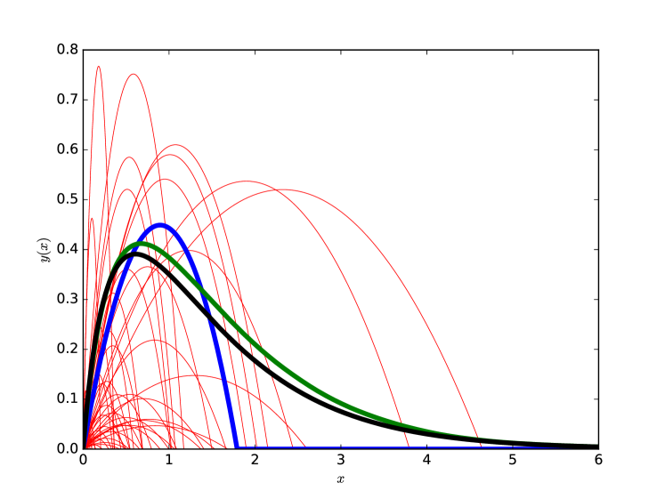
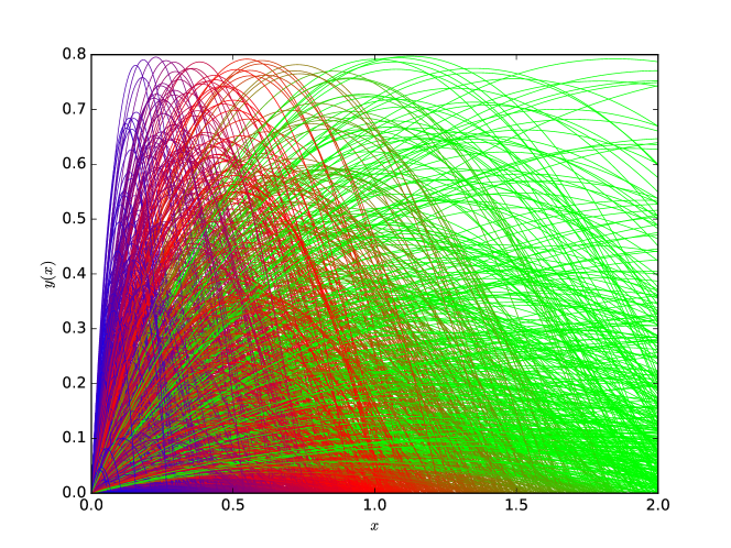
For the “ideal” case where the projectile hits right into $\bar{R}$ the maximum $y$ will always occur at $x=\bar{R}/2$. By using that $\left<\bar{R}\right>_{v_{0},\theta_{0}}\sim 1.09$ we have that $\bar{R}/2\sim 0.55$, which is close to the mentioned numerical value. For the case of $\bar{R}=1$, the maximum of Eqs. 13, and 18 corresponds to 0.61 and 2.74 respectively, which are in excellent agreement with the data provided by the simulations (0.65 and 2.72, respectively). A larger number of curves is displayed in Fig. 2, by using a color-scale scheme. Here the curves are colored according to their range $R$: if $R$ is close to 0, $\bar{R}$, and 2$\bar{R}$ then the colors will be graduated from blue, red, and green respectively.

Figure 2: Color map for a large number of trajectories, using initial conditions sampled from Eq. 9. Values of $R$ near to 0, 1, and 2, are colored from blue, to red, to green respectively.

The histogram of $R$ compatible with $\bar{R}$ according to Eq. 5 is presented in Fig. 3. We observe a close agreement with the exponential probability distribution in Eq. 19 (solid line).

Figure 3: $\bar{R}$ Statistical distribution of ranges $R$ from the data distribution. The solid line is the exponential distribution in Eq. 19

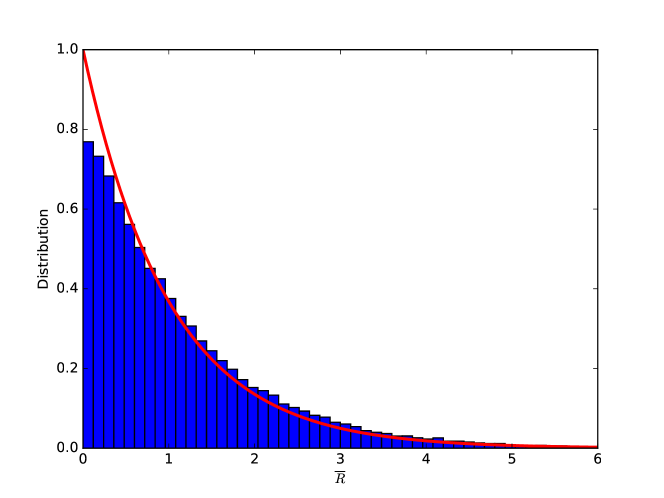
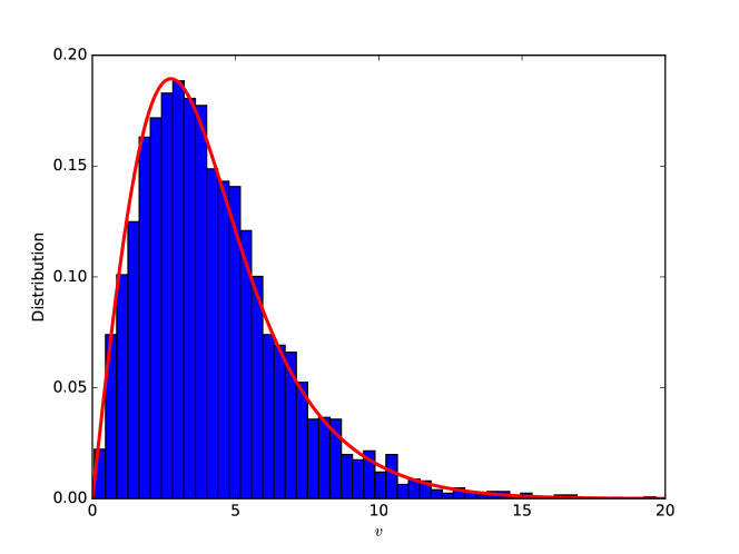
Fig. 4 shows the histogram of the initial velocity $v_{0}$, having in principle values ranged from 0 to $\infty$. However it is important to notice that this quantity is still constrained by the average range $\bar{R}$, as is presented in Eq. 18. We can see a narrow and well-defined distribution centered in 2.7 m/s. The red color line represents the analytical distribution computed using numerical integration, given by Eq. 18. There is a good agreement between the Monte Carlo data and the predicted numerical distribution.

Figure 4: $v$ Distribution of initial velocities from the generated Monte Carlo data. We observe a narrow and well-defined distribution centered in 2.7 m/s. The red color line, represents the analytical distribution computed using numerical integration, given by Eq. 18.

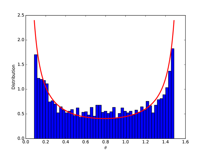
As a contrast, the angle $\theta$ is more confined, for both physical and numerical reasons. From a physics point of view, angles larger than $\frac{\pi}{2}$ do not make sense for the projectile motion, and from a numerical point of view, the singularity of the solutions (Eq. 8) is evident for the case of $\theta$=0 and $\theta=\frac{\pi}{2}$. Fig. 5 presents the results of the angular distribution. The red line corresponds to the distribution provided by Eq. 16. A good agreement is observed in the angle distribution.

Figure 5: $\theta$ Distribution of initial angles $\theta_{0}$ from the generated Monte Carlo data. The red line corresponds to the distribution provided by Eq. 16.

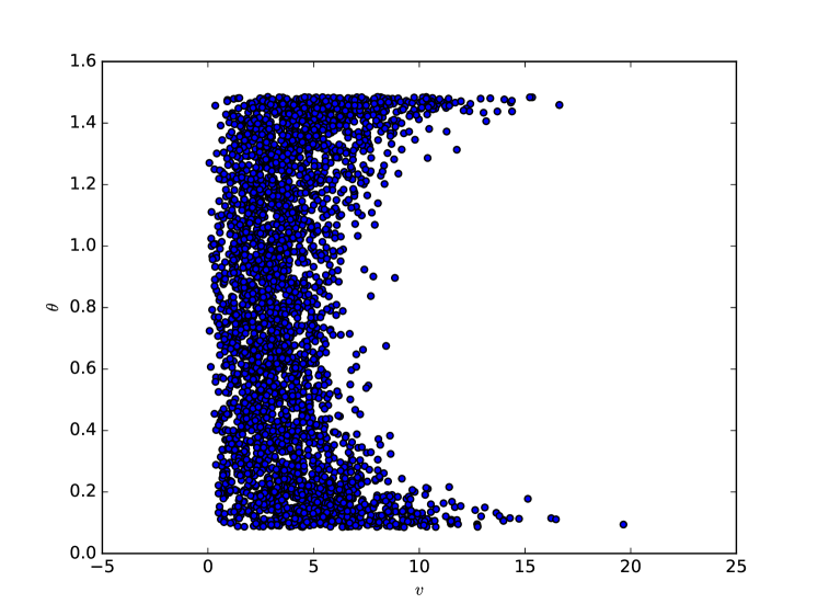
Another interesting point is to evaluate the possible correlations between initial speed and angle, and for this we present in Fig. 6 the scatter plot of $(v_{0},\theta_{0})$ pairs. We see that for slow speeds the angle distribution is uniform, while for high speeds it becomes concentrated around $\theta$=0 and $\theta$=$\pi$/2. This is expected, as for high speeds the requirement of a low value of $\bar{R}$ constrains the angles to approach $\sin 2\theta\approx 0$.

Figure 6: $\theta$ Scatter plot of initial conditions $\theta_{0}$ and $v_{0}$. We see that for slow speeds the angle distribution is uniform, while for high speeds it becomes concentrated around $\theta$=0 and $\theta$=$\pi$/2.

5 Conclusions

By the use of the Maximum Entropy formalism, we have shown that the problem of inferring the initial conditions for determistic physics problems is far from being intractable. MaxEnt allows us to provide a concise mathematical statement of the inverse kinematic problem, which was solved both analytically and numerically via Monte Carlo simulation. We have described the details of the procedure to infer the probability distribution of initial conditions using the projectile motion as an example. Statistical sampling using Monte Carlo (Metropolis-Hastings) was made in order to check the validity of our analytical results. Our results constitute a proof-of-concept of the Maximum Entropy formalism applied to solve the initial conditions of deterministic kinematic and dynamical problems, given information of quantities measured at posterior times.

Bibliography

- [1] Edwin T Jaynes. Probability theory: The logic of science. Cambridge university press, 2003.
- [2] T. M. Cover and J. A. Thomas. Elements of Information Theory. John Wiley and Sons, 2006.
- [3] Seán M Stewart. On the trajectories of projectiles depicted in early ballistic woodcuts. European Journal of Physics, 33(1):149, 2012.
- [4] Mustafa Turkyilmazoglu. Highly accurate analytic formulae for projectile motion subjected to quadratic drag. European Journal of Physics, 37(3):035001, 2016.
- [5] Jeffrey C. Hayen. Projectile motion in a resistant medium. International Journal of Non-Linear Mechanics, 38(3):357 – 369, 2003.
- [6] Seán M. Stewart. Linear resisted projectile motion and the lambert w function. American Journal of Physics, 73(3):199–199, 2005.
- [7] Daniel A Morales. Exact expressions for the range and the optimal angle of a projectile with linear drag. Canadian Journal of Physics, 83(1):67–83, 2005.
- [8] G. W. Parker. Projectile motion with air resistance quadratic in the speed. American Journal of Physics, 45(7):606–610, 1977.
- [9] Herman Erlichson. Maximum projectile range with drag and lift, with particular application to golf. American Journal of Physics, 51(4):357–362, 1983.
- [10] Nicholas P. Linthorne and David J. Everett. Soccer. Sports Biomechanics, 5(2):243–260, 2006.
- [11] Kim Williams and Marco Giorgio Bevilacqua. Leon battista alberti’s bombard problem in ludi matematici: Geometry and warfare. The Mathematical Intelligencer, 35(4):27–38, 2013.
- [12] Riccardo Borghi. Trajectory of a body in a resistant medium: an elementary derivation. European Journal of Physics, 34(2):359, 2013.
- [13] E. T. Jaynes. Information theory and statistical mechanics. Phys. Rev., 106:620–630, May 1957.
- [14] Steve Pressé, Kingshuk Ghosh, Julian Lee, and Ken A Dill. Principles of maximum entropy and maximum caliber in statistical physics. Reviews of Modern Physics, 85(3):1115, 2013.
- [15] D. S. Sivia and J. Skilling. Data Analysis: A Bayesian Tutorial. Oxford University Press, 2006.
- [16] Sergio Davis, Joaquín Peralta, Yasmín Navarrete, Diego González, and Gonzalo Gutiérrez. A bayesian interpretation of first-order phase transitions. Foundations of Physics, 46(3):350–359, 2016.
- [17] Leonard E. Baum and Melvin Katz. Convergence rates in the law of large numbers. Transactions of the American Mathematical Society, 120(1):108–123, 1965.
- [18] Kenneth L Judd. The law of large numbers with a continuum of iid random variables. Journal of Economic Theory, 35(1):19 – 25, 1985.
- [19] D. Gamerman and H. F. Lopes. Markov Chain Monte Carlo: Stochastic Simulation for Bayesian Inference. Taylor and Francis, 2006.