Constraining the dark energy models with H(z) data: an approach independent of $H_{0}$

Abstract

We study the performance of the latest $H(z)$ data in constraining the cosmological parameters of different cosmological models, including that of Chevalier-Polarski-Linder $w_{0}w_{1}$ parametrization. First, we introduce a statistical procedure in which the chi-square estimator is not affected by the value of the Hubble constant. As a result, we find that the $H(z)$ data do not rule out the possibility of either non-flat models or dynamical dark energy cosmological models. However, we verify that the time varying equation-of-state parameter $w(z)$ is not constrained by the current expansion data. Combining the $H(z)$ and the Type Ia supernova data we find that the $H(z)$/SNIa overall statistical analysis provides a substantial improvement of the cosmological constraints with respect to those of the $H(z)$ analysis. Moreover, the $w_{0}-w_{1}$ parameter space provided by the $H(z)$/SNIa joint analysis is in a very good agreement with that of Planck 2015, which confirms that the present analysis with the $H(z)$ and SNIa probes correctly reveals the expansion of the Universe as found by the team of Planck. Finally, we generate sets of Monte Carlo realizations in order to quantify the ability of the $H(z)$ data to provide strong constraints on the dark energy model parameters. The Monte Carlo approach shows significant improvement of the constraints, when increasing the sample to 100 $H(z)$ measurements. Such a goal can be achieved in the future, especially in the light of the next generation of surveys.

I Introduction

The general picture of the Cosmos, as it is established by the analysis of the recent cosmological data (see Planck16 and references therein), is described with a cosmological scenario that consists $\sim 30\%$ of matter (baryonic and dark) and the rest corresponds to the so called dark energy (DE). This mysterious component of the cosmic fluid plays an eminent role in cosmological studies because it is responsible for the accelerated expansion of the Universe. Also, current observations seem to favor an isotropic, homogeneous and spatially flat universe.

During the last decades, different classes of theoretical models have been introduced in order to explain the accelerating Universe, giving rise to a scholastic debate about what is the exact description and the key points of each scheme. One of the fundamental questions of modern cosmology that subsequently emerges is what is the model that best describes the accelerated expansion of the universe, maartens2010 . A prominent path in order to distinguish the various cosmological models is to probe the cosmic history Probes of the universe, using either the luminosity distance of standard candles or the angular diameter distance of standard rulers.

In general, the geometrical probes used to map the cosmic expansion history involve a combination of standard candles (SNIa Suzuki:2011hu ; Betoule14 ), GRBs GRB , HII Plionis2011 ; Chavez2016 ), standard rulers (clusters, CMB sound horizon detected through Baryon Acoustic Oscillations (BAO); Blake ; Alam2016 ), the CMB angular power spectrum Planck16 and recently, data from gravitational wave measurements, the so called ’standard sirens’, Calabrese2016 . Alternatively, dynamical probes of the expansion history based on measures of the growth rate of matter perturbations (for recent studies see Nes17 and references therein) are also used towards tracing the cosmic expansion and they are confined to relatively low redshifts similar to those of Type Ia supernova data $z\simeq 1.4$. The aforementioned observations probe the integral of the Hubble parameter $H(z)$, hence they give us indirect information for the cosmic expansion. Also, it is worth noting that in some cases the data suffer from the so called circularity problem, the fact that one needs to impose a fiducial cosmology in order to be able to define the data (see for example Wang2005 , Shapiro2006 ).

Among the large body of cosmological data the only data-set that provides a direct measurement of the cosmic expansion is the $H(z)$ sample and indeed a plethora of papers have been published (e. g. Samushia2006 , Farooq13 , ChimentoRicharte2013 , Ferreira et al. (2013), Capozziello et al. (2014), GruberLuongo14 , Forte (2014), Dankiewicz et al. (2014), Cai et al. (2014), Melia2015 , Chen et al. (2016a), Mukherjee & Banerjee (2016), Farooq16 , Saridakis , Cardasian , Saridakisf(R) ) which determine the dynamical characteristics of various DE cosmological models, including those of modified gravity. Today, the most recent $H(z)$ data trace the cosmic expansion rate up to redshifts of order $z\simeq 2.4$, while there are proposed methods SantageLoeb which potentially could expand the $H(z)$ measurements to $z\leq 5$. As expected using the $H(z)$ data in constraining the cosmological models via the standard likelihood analysis, one has to deal with the Hubble constant, namely $H_{0}$. However, the best choice of the value of $H_{0}$ is rather uncertain. Indeed, several studies on the determination of the Hubble constant have indicated a $\sim 3.1\sigma$ tension between the value obtained by the Planck team (see Planck16 ), namely $H_{0}=67.8\pm 0.9$ Km/s/Mpc and the results provided by the SNIa project (Riess et al. Riess16 ) of $H_{0}=73.24\pm 1.74$ Km/s/Mpc. In order to alleviate this problem we propose in the current work a statistical method which is not affected by the value of $H_{0}$.

The structure of the article is as follows: In Sec. II we present the $H(z)$ data used and the related statistical analysis. At the beginning of Sec. III we describe the main properties of the most basic DE models and then we focus on the cosmological constrains. In Sec. IV we discuss the Monte Carlo simulations used towards planning future $H(z)$ measurements in order to place better constraints on the DE model parameters. Finally, in Sec. V we provide a detailed discussion of our results and we summarize our conclusions in Sec. VI.

Table 1: The observational data-set that was used in this paper. The data-set, compiled by Farooq et al, 2016 Farooq16 consists of $N=38$ observations.

$z$	$H(z)[{\rm Km/s/Mpc}]$	$\sigma_{H}[{\rm Km/s/Mpc}]$	Method/Ref.
0.070	69.0	19.6	Zhang2014
0.090	69.0	12.0	Simon2005
0.120	68.6	26.2	Zhang2014
0.170	83.0	8.0	Simon2005
0.179	75.0	4.0	Moresco2012
0.199	75.0	5.0	Moresco2012
0.200	72.9	29.6	Zhang2014
0.270	77.0	14.0	Simon2005
0.280	88.8	36.6	Zhang2014
0.352	83.0	14.0	Moresco2012
0.380	81.5	1.9	Alam2016
0.3802	83.0	13.5	Moresco2016
0.400	95.0	17.0	Simon2005
0.4004	77.0	10.2	Moresco2016
0.4247	87.1	11.2	Moresco2016
0.440	82.6	7.8	Blake2012
0.4497	92.8	12.9	Moresco2016
0.4783	80.9	9.0	Moresco2016
0.480	97.0	62.0	Stern2010
0.510	90.4	1.9	Alam2016
0.593	104.0	13.0	Moresco2012
0.600	87.9	6.1	Blake2012
0.610	97.3	2.1	Alam2016
0.680	92.0	8.0	Moresco2012
0.730	97.3	70.0	Blake2012
0.781	105.0	12.0	Moresco2012
0.875	125.0	17.0	Moresco2012
0.880	90.0	40.0	Stern2010
0.900	117.0	23.0	Simon2005
1.037	154.0	20.0	Moresco2012
1.300	168.0	17.0	Simon2005
1.363	160.0	33.6	Moresco2015
1.430	177.0	18.0	Simon2005
1.530	140.0	14.0	Simon2005
1.750	202.0	40.0	Simon2005
1.965	186.5	50.4	Moresco2015
2.340	222.0	7.0	Delubac2015
2.360	226.0	8.0	Font-Ribera2014

Figure 1: The redshift (upper panel) and the relative error (lower panel) distributions of our dataset.

II Statistical analysis with H(z) data

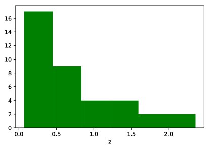
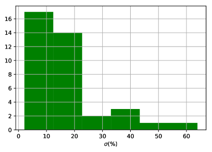
In this section we discuss the details of the statistical analysis and on the observational sample that we utilize in order to place constraints on the cosmological parameters. In particular, we use the cosmic expansion data as collected by Farooq et al. Farooq16 (see Table I and the corresponding references) for which the Hubble parameter is available as a function of redshift. Notice, that the $H(z)$ sample contains 38 entries in the following redshift range $0.07\leq z\leq 2.36$. In Fig.1, we present the normalized redshift distribution of the $H(z)$ data and the corresponding distribution of the relative uncertainty $\sigma(\%)=\sigma_{H(z_{i})}/H(z_{i})$. Also, we find no significant correlation between $\sigma$ and redshift in that range.

First let us assume that we have a dark energy model that includes $n$-free parameters, provided by the statistical vector $\phi^{\mu}=(\phi^{0},\phi^{1},...\phi^{n})$. In order to put constraints on $\phi^{\mu}$ we need to implement a standard $\chi^{2}$-minimization procedure, which in our case is written as

$$\chi^{2}(\phi^{\mu})=\sum_{i=1}^{N}\left[\frac{H_{D}(z_{i})-H_{M}(z_{i},\phi^{\mu})}{\sigma_{i}}\right]^{2}$$ (1)

where $H_{D}(z_{i})$, $\sigma_{i}$ are the observational data and the corresponding uncertainties at the observed redshift, $z_{i}$. The capital letters $M$ and $D$ stand for model and data respectively. In this case the theoretical Hubble parameter is written as

$$H_{M}(z,\phi^{\mu})=H_{0}E(z,\phi^{\mu+1})$$ (2)

where $H_{0}$ is the current value of Hubble parameter, namely the Hubble constant, $E(z)$ is the normalized Hubble function and the vector $\phi^{\mu}$ contains the cosmological parameters. In this framework we observe that the statistical vector becomes $\phi^{\mu}=(H_{0},\phi^{\mu+1})$, where the components $\phi^{\mu+1}$ contains the free parameters which are related with the matter density, spatial curvature and dark energy.

Therefore, in order to proceed with the statistical analysis we need to either know the exact value of the Hubble constant or having it as a free parameter.The most recent results on the determination of the Hubble constant have found a $\sim 3.1\sigma$ tension between the value obtained by SN Ia project (Riess et al. Riess16 ) of $H_{0}=73.24\pm 1.74$ Km/s/Mpc and the results from Planck (see Planck16 ) of $H_{0}=67.8\pm 0.9$ Km/s/Mpc. The Hubble constant problem has inspired us to propose a technique which provides the chi-square estimator independent from the value of $H_{0}$. At this point we present the basic ingredients towards marginalizing $\chi^{2}$ over $H_{0}$. Indeed, inserting (2) into (1) the latter equation simply becomes

$$\chi^{2}(\phi^{\mu})=AH_{0}^{2}-2BH_{0}+\Gamma,$$ (3)

where

$$A=\sum_{i=1}^{N}\frac{E^{2}(z_{i})}{\sigma_{i}^{2}}$$

$$B=\sum_{i=1}^{N}\frac{E(z_{i})H_{D}(z_{i})}{\sigma_{i}^{2}}$$

$$\Gamma=\sum_{i=1}^{N}\frac{H_{D}(z_{i})^{2}}{\sigma_{i}^{2}}$$

In this context the corresponding likelihood function is written as

$$\mathcal{L}=e^{-x^{2}/2}\Rightarrow\mathcal{L}={\rm exp}\left[\frac{AH_{0}^{2}-2BH_{0}+\Gamma}{2}\right]$$ (4)

or

$$\mathcal{L}(D|\phi^{\mu},M)={\rm exp}\left[\frac{A\left(H_{0}-\frac{B}{A}\right)^{2}-\frac{B^{2}}{A}+\Gamma}{2}\right]\;.$$

Using Bayes’s theorem and marginalizing over $H_{0}$ we arrive at

$$p(\phi^{\mu}|D,M)=\frac{1}{p(D|M)}\int e^{-\frac{A(H_{0}-B/A)^{2}-B^{2}/A+\Gamma}{2}}dH_{0}\;.$$ (5)

Furthermore, considering that $H_{0}$ lies in the range $H_{0}\in(0,+\infty)$, introducing the variable $y=H_{0}-B/A$ and utilizing flat priors $p(\phi^{\mu}|M,H_{0})=1$ we obtain after some simple calculations

$$p(\phi^{\mu}|D,M)=\frac{1}{p(D|M)}e^{-\frac{1}{2}\left(\Gamma-B^{2}/A\right)}\int_{-\frac{B}{A}}^{+\infty}e^{-\frac{A}{2}y^{2}}dy$$ (6)

or

$$p(\phi^{\mu}|D,M)=\frac{1}{p(D|M)}e^{-\frac{1}{2}\left[\Gamma-\frac{B^{2}}{A}\right]}\sqrt{\frac{\pi}{2A}}\left[1+{\rm erf}\left(\frac{B}{\sqrt{2A}}\right)\right],$$ (7)

where ${\rm erf}(x)=\frac{2}{\sqrt{\pi}}\int_{0}^{x}e^{-y^{2}}dy$ is the error function. Lastly, it is easy to show that the above likelihood function corresponds to the following marginalized ${\tilde{\chi}}^{2}_{H}$ function:

$${\tilde{\chi}}^{2}_{H}(\phi^{\mu+1})=\Gamma-\frac{B^{2}}{A}+\ln A-2\ln\left[1+{\rm erf}\left(\frac{B}{\sqrt{2A}}\right)\right]\;.$$ (8)

where we have ignored the constant ${\rm ln}(\pi/2)$, since it does not play a role during the minimization procedure.

Obviously, the statistical estimator (8) does not suffer from the Hubble constant problem. Indeed, instead of minimizing $\chi^{2}$ we now use the marginalized ${\tilde{\chi}}^{2}_{H}$ function which is independent of $H_{0}$ and thus we do not need to impose in the statistical analysis an a priori value for the Hubble constant, as usually done in many other studies of this kind.

Bellow, we test the performance of the current statistical procedure at the expansion level using some well known dark energy models.

III Fitting models to $H(z)$ data

In this section we present the expansion rate of the Universe in the context of the most basic DE models whose free parameters are constrained following the procedure of the previous section. Due to the fact that the $H(z)$ data are well inside in the matter dominated era we can neglect the radiation term from the Hubble expansion.

Let us now briefly discuss the cosmological models explored in the present study.

• Non-flat $\Lambda$CDM model. In this case the Hubble parameter is given by

  $$E(z,\phi^{\mu+1})=\left[\Omega_{m0}(1+z)^{3}+\Omega_{\Lambda 0}+\Omega_{K0}(1+z)^{2}\right]^{1/2},$$ (9)

  where $\Omega_{K0}$ is the dimensionless curvature density parameter at the present time which is defined as $\Omega_{K0}=1-\Omega_{m0}-\Omega_{\Lambda 0}$, hence the cosmological vector takes the form $\phi^{\mu+1}=(\Omega_{m0},\Omega_{\Lambda 0})$.

• wCDM model. In this spatially flat model the equation of state parameter $w_{d}=p_{d}/\rho_{d}$ is constant wCDM , where $\rho_{d}$ is the density and $p_{d}$ is the pressure of the dark energy fluid respectively. Under the latter conditions the normalized Hubble function is

  $$E(z,\phi^{\mu+1})=\left[\Omega_{m0}(1+z)^{3}+\Omega_{d0}(1+z)^{3(1+w)}\right]^{1/2},$$ (10)

  where $\Omega_{d0}=1-\Omega_{m0}$ and thus the cosmological vector is $\phi^{\mu+1}=(\Omega_{m0},w)$.

• CPL model. This cosmological model was first introduced in the literature by Chevalier-Polarski-Linder Linder03 , ChevallierPolarski . Here the equation of state parameter is allowed to vary with redshift and it is written as a first order Taylor expansion around the present epoch, $w(a)=w_{0}+w_{1}(1-a)$ with $a=1/(1+z)$. Therefore, the dimensionless Hubble parameter takes the following form

  $$E(z,\phi^{\mu+1})=\left[\Omega_{m0}(1+z)^{3}+\Omega_{d0}X(z)\right]^{1/2},$$ (11)

where

$$X(z)=(1+z)^{3(1+w_{0}+w_{1})}{\rm exp}\left(-3w_{1}\frac{z}{z+1}\right)$$

and $\Omega_{d0}=1-\Omega_{m0}$. In this case the vector of the model parameters is $\phi^{\mu+1}=(\Omega_{m0},w_{0},w_{1})$.

For the non-flat $\Lambda$CDM model the likelihood function peaks at $(\Omega_{m0},\Omega_{\Lambda 0})=(0.250^{+0.039}_{-0.043},0.693^{+0.147}_{-0.186})$ with ${\tilde{\chi}^{2}}_{H,\rm min}/df\simeq 0.639$ ($df$ are the degrees of freedom). Also, based on $\Omega_{K0}=1-\Omega_{m0}-\Omega_{\Lambda 0}$ we find $\Omega_{K0}=0.057^{+0.142}_{-0.152}$. Our constraints are in agreement within $1\sigma$ errors to those of Farooq et al. Farooq16 who found, using the same $H(z)$ data, $(\Omega_{m0},\Omega_{\Lambda 0})=(0.23,0.60)$ for $H_{0}=68$ Km/s/Mpc and $(\Omega_{m0},\Omega_{\Lambda 0})=(0.25,0.78)$ for $H_{0}=73.24$ Km/s/Mpc respectively. Recently, Jesus et al. Jesus found $H_{0}=69.5\pm 2.5$Km/s/Mpc, $\Omega_{m0}=0.242\pm 0.036$ $\Omega_{\Lambda 0}=0.256\pm 0.14$, while using the Riess et al. Riess11 prior $H_{0}=73.8$Km/s/Mpc they found $0.21\leq\Omega_{m0}\leq 0.32$ and $0.65\leq\Omega_{\Lambda 0}\leq 0.99$.

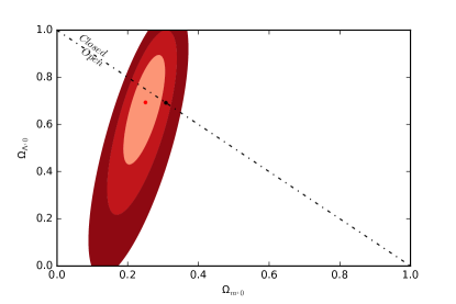
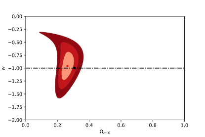
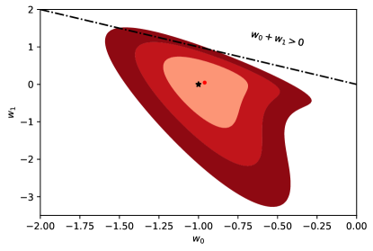
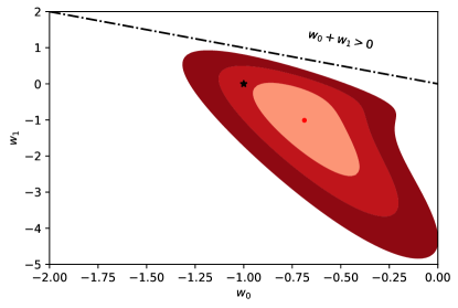
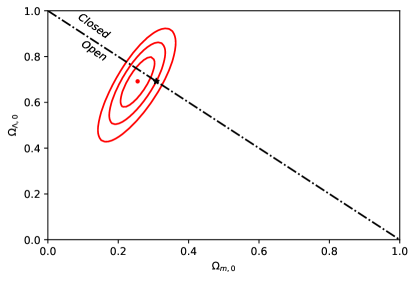
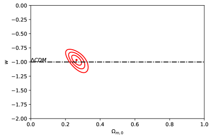
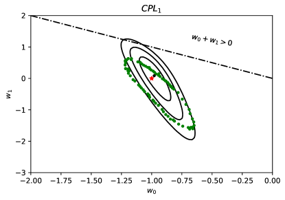
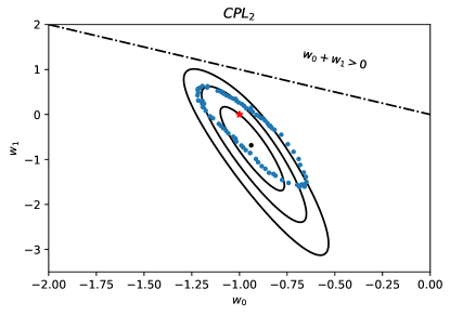
In the case of wCDM cosmological model the results of the minimization analysis are $(\Omega_{m0},w)=(0.262^{+0.042}_{-0.037},-0.96^{+0.275}_{-0.270})$ with ${\tilde{\chi}}^{2}_{\rm min}/df\simeq 0.64$. For comparison Farooq et al. Farooq16 obtained $(\Omega_{m0},w_{0})=(0.26,-0.86)$ for $H_{0}=68$ Km/s/Mpc and $(\Omega_{m0},w_{0})=(0.24,-1.06)$ for $H_{0}=73.24$ Km/s/Mpc respectively. Lastly, for the CPL parametrization we find: ${\tilde{\chi}}^{2}_{\rm min}/df\simeq 0.64$ and $(w_{0},w_{1})=(-0.960\pm{0.171},0.047\pm{0.425})$, where we have set $\Omega_{m0}=0.262$. We repeat our analysis by using the $\Omega_{m}$-prior derived originally by the Planck team Planck16 . Specifically, if we impose $\Omega_{m0}=0.308$ then we obtain $(w_{0},w_{1})=(-0.687\pm{0.123},-1.009\pm{0.598})$ with ${\tilde{\chi}}^{2}_{H,\rm min}/df\simeq 0.66$. Notice, that in Table II we provide a more compact presentation of our statistical results. In Fig. 2 we plot the 1$\sigma$, 2$\sigma$ and $3\sigma$ confidence contours in the $(\Omega_{m0},\Omega_{\Lambda 0})$ and $(\Omega_{m0},w)$ planes for non-flat $\Lambda$CDM (upper panel) and wCDM (bottom panel) models respectively. We observe that our best-fit values are almost $\sim 1\sigma$ away, from the values provided by the Planck team Planck16 (see stars in Fig. 2). Moreover, in Fig. 3 we show the $(w_{0},w_{1})$ contours for the CPL model by using $\Omega_{m0}=0.262$ (upper panel) and $\Omega_{m0}=0.308$ (bottom panel). The stars in Fig. 3 corresponds to the solution $(w_{0},w_{1})=(-1,0)$. As expected, we find that the parameter $w_{0}$ is degenerate with respect to $w_{1}$, implying that the time varying equation-of-state parameter $w(z)$ is not constrained by this analysis.

Figure 2: The likelihood contours for $\Delta{\tilde{\chi}}^{2}={\tilde{\chi}}^{2}_{H}-{\tilde{\chi}}^{2}_{H,\rm min}$ equal to 1$\sigma$ (2.32), 2$\sigma$ (6.18) and 3$\sigma$ (11.83) confidence levels. The red dot corresponds to the best-fit solutions. Upper panel: the contours of the non-flat $\Lambda$CDM model, in the $(\Omega_{m0},\Omega_{\Lambda})$ plane. The dashed line represents the $\Omega_{m0}+\Omega_{\Lambda}=1$ line. Here the best fit point is $(\Omega_{m0},\Omega_{\Lambda})=(0.250,0.693)$. Lower panel: the wCDM model in the $(\Omega_{m0},w)$ plane. The best fit solution is $(\Omega_{m0},w)=(0.262,-0.960)$. The dashed curve corresponds to $w=-1$. Notice, that stars show the best-fit solution provided by the Planck team, Planck16 for the flat $\Lambda$CDM model.

Figure 3: The likelihood contours $\Delta{\tilde{\chi}}^{2}={\tilde{\chi}}^{2}_{H}-{\tilde{\chi}}^{2}_{H,\rm min}$ in the case of CPL model. Upper panel: Here we utilize $\Omega_{m0}=0.262$ from the first panel of Table II. Bottom panel: Here we use $\Omega_{m0}=0.308$ from Planck, Planck16 . Notice that stars corresponds to flat $\Lambda$CDM model $(w_{0},w_{1})=(-1,0)$.

Figure 4: The $H(z)$/SNIa joint likelihood contours. The upper panel shows the solution space for the non-flat $\Lambda$CDM model, while the lower panel corresponds to wCDM model. The dashed line corresponds to $w=-1$. The red dot corresponds to the best-fit solutions. The black star shows the solution of Planck Planck16 .

Figure 5: The joint SNIa and $H(z)$ likelihood contours in the ($w_{0},w_{1}$) plane for $\Omega_{m0}=0.262$ (upper panel) and $\Omega_{m0}=0.308$ (lower panel). The solid black dots correspond to the best fit parameters. We also show the theoretical $\Lambda$CDM $(w_{0},w_{1})=(-1,0)$ values (star points). The dot-dashed line corresponds to $w_{0}+w_{1}=0$. Finally, the area of green/blue dots borrowed from Planck Planck16 .

III.1 Joint Analysis with SN Ia

Although the $H(z)$ data provide a direct measurement of the expansion of the Universe, due to their large errors with respect to the SN Ia data, various authors preferred to utilize the latter data in order to constrain the cosmological parameters. Here we want to combine $H(z)$ and SN Ia in order to study the performance of the $H(z)$ data (as they stand today, namely 38 entries) with that of SN Ia data. In particular, we use the Union 2.1 set of 580 SN Ia of Suzuki et al. Suzuki:2011hu . Concerning the chi-square estimator of the SN Ia we utilize the method of Nes05 , where the form of ${\tilde{\chi}}^{2}_{\rm Sn}$ is independent of $H_{0}$ (see also Ref.Chavez2016 and references therein). In this framework, the overall likelihood function is given by the product of the individual likelihoods according to:

$$\cal L_{\rm tot}={\cal L}_{\rm sn}\times{\cal L}_{H}$$

which translates in an addition for the total $\chi^{2}_{\rm tot}$:

$$\chi^{2}_{\rm tot}={\tilde{\chi}}^{2}_{\rm sn}+{\tilde{\chi}}^{2}_{H}$$

The results based on the joint analysis of $H(z)$/SNIa data are given in Figs. (4-5) and listed in the second panel of Table II. It becomes clear that the addition of the SNIa data in the likelihood analysis improves substantially the statistical results. Overall, we find that the $H(z)$/SNIa joint analysis increases the Figure of Merit (FoM: for definition see below) by a factor of $\sim 2.5$ with respect to that of $H(z)$ analysis. Therefore, the combined analysis of the $H(z)$ data with SNIa reduces significantly the parameter space, providing tight constraints on the non-flat $\Lambda$CDM and wCDM models respectively. In particular, for the former model the total likelihood function peaks at $(\Omega_{m0},\Omega_{\Lambda 0})=(0.255\pm{0.02},0.692\pm{0.045})$ with $\chi^{2}_{\rm tot,min}/df\simeq 0.950$, while for the latter cosmological model we find $(\Omega_{m0},w)=(0.264\pm{0.015},-0.965\pm{0.046})$ with $\chi^{2}_{\rm tot,min}/df\simeq 0.950$. Concerning the CPL model we find that although the area of $w_{0}-w_{1}$ contours is significantly reduced, the degeneracy between $w_{0}$ and $w_{1}$ persists also in the joint analysis. However, what is specifically interesting is that for the CPL model the $H(z)$/SNIa contours are in very good agreement with those of Planck TT, lowP CMB data and external (BAO, JLA, $H_{0}$) data, Planck16 (see solid circles in Fig.5), which confirms that our analysis with the $H(z)$ and SNIa probes correctly reveals the expansion history of the Universe as provided by the Planck team.

Concluding this section it is interesting to mention that recently, Yu et al. Yu17 introduced the covariance matrix of three BAO $H(z)$ measurements Alam2016 in the $H(z)$ analysis. Using this covariance matrix we have re-done our statistical analysis and in Table III we provide the corresponding constraints, which are in agreement (within 1$\sigma$ errors) with those of Table II. Notice, that in the appendix we have generalized the statistical methodology of section II in the presence of the covariance matrix.

IV Strategy to improve the cosmological constrains using the $H(z)$ data

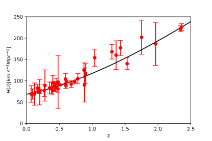
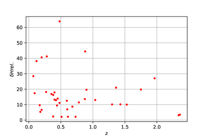
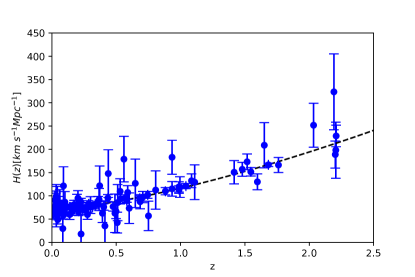
From the previous analysis it becomes clear that an important question that we need to address is the following: What is the strategy for the recovery of the dark energy equation of state using the direct measurements of the Hubble expansion? In this section we proceed with our investigation towards studying the effectiveness of utilizing $H(z)$ measurements to constrain the equation of state parameter. Specifically, our aim is to test how better can we go in placing cosmological constraints by increasing the current $H(z)$ sample from 38 to 100. In order to achieve such a goal, we produce sets of Monte Carlo simulations with which we quantify our ability to recover the input cosmological parameters of a fiducial cosmological model, namely $(\Omega_{m0},\Omega_{K0},w_{0},w_{1})=(0.25,0,-1,0)$ with $H_{0}=68.75$ Km/s/Mpc. In the upper panel of Fig. 6 we present the evolution of the Hubble parameter of the reference model (see solid) line and on top of that we plot the $H(z)$ data (solid points). In the lower panel of Fig  6 we show the distribution of $100(\%)\times|H_{D}-H_{\rm ref}|/H_{D}$ as a function of redshift (see below), where $H_{D}$ and $H_{\rm ref}$ are the Hubble parameters of the data and the reference cosmology respectively. We verify that the differences $\delta H=|H_{D}-H_{\rm ref}|$ are not correlated with redshift.

Figure 6: Upper panel: Comparison of the observed (red points Farooq16 ) and theoretical evolution of the reference Hubble parameter, $H(z)$, using $(\Omega_{m0},\Omega_{K0},w_{0},w_{1})=(0.25,0,-1,0)$ and $H_{0}=68.75$Km/s/Mpc. The reference cosmology is represented by the solid curve. Lower panel: The distribution of $\delta H=|H_{D}-H_{\rm ref}|$. Notice, that $H_{D}(z)$ indicates the observed Hubble parameter, while $H_{\rm ref}(z)$ is the Hubble function of the fiducial cosmology.

Now, we develop an algorithm that generates different number of mock $H_{\rm MC}(z)$ measurements following the redshift and the error distributions of the real $H(z)$ data (see Figures 1 and 2). Thus, our aim is to obtain the value of $H_{\rm MC}$ as well as the corresponding $1\sigma$ error by calibrating the mock $H(z)$ sample from the real $H(z)$ data in which $0.07\leq z\leq 2.36$. More specifically, we implement the following steps:

First, from the redshift interval $[0.07,2.36]$ we choose a redshift $z_{\rm ran}$ by randomly sampling the observed redshift distribution (see Fig.1). For this ”random” redshift we define the measured Hubble parameter $H_{D}(z_{\rm ran})$ and the ideal Hubble parameter $H_{\rm ref}(z_{\rm ran})$ from the reference cosmology. Second, in order to take into account the deviation of the observed Hubble parameter from the reference cosmology we are randomly sampling the distribution of the differences $\delta H$ (see lower panel of Fig. 6) between the data and the fiducial cosmological model. Once, steps (1) and (2) are completed for all mock data used, the mock Hubble parameter $H_{\rm MC}$ is selected from the normal distribution ${\cal N}(H_{\rm ref},\sigma^{2}_{\rm ran})$. Finally, performing a trial and error procedure we have confirmed that by assigning to each mock Hubble parameter $H_{\rm MC}$ the individual error $\sigma_{\rm ran}=\sqrt{\sigma_{H}^{2}+\delta H^{2}}$ we recover the contours of the reference model and thus the mock $H(z)$ data contain the following simulated triads $\{z_{\rm ran},H_{\rm MC},\sigma_{\rm ran}\}_{i}$, where $i=1,..N$ and $N\in[38,120]$. For the benefit of the reader in Fig.7 we plot the mock Hubble parameter as a function of redshift. Notice that in this case the mock sample constraints $N=100$ entries. This figure can be compared with that of the observed $H(z)$ data (see upper panel of Fig. 6).

Figure 7: The mock Hubble parameter as a function of redshift. In this case the mock data-set constraints $N=100$ entries. The dashed line corresponds to $\Lambda$CDM model with $(H_{0},\Omega_{m0},\Omega_{\Lambda 0})=(68.5,0.25,0.693)$.

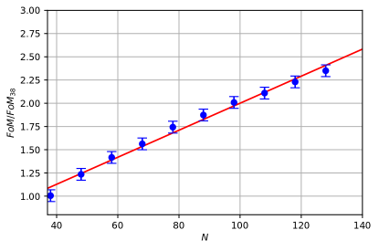
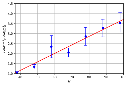
Now, based on the mock data we attempt to measure the effectiveness of the $H(z)$ measurements in constraining the cosmological parameters. Therefore, we calculate the well known Figure-of-Merit (FoM) in the solution space. The FoM is a useful tool because it provides an assess how constraining the likelihood analysis of the $H(z)$ data can be. We have defined the FoM as the inverse of the enclosed area of the 2$\sigma$ contour in the parameter space of any two degenerate cosmological parameters, namely $\Omega_{m0}-\Omega_{\Lambda 0}$ and $w_{0}-w_{1}$. Of course, the higher the FoM is, the more constraining the model. We generate 100 Monte-Carlo simulations for each selected number ($N=38,40,..120$) of mock $H(z)$ data, and the corresponding results are shown in Fig. 8. In this figure we plot the ratio between the simulation FoM and that of the present sample of 38 $H(z)$ measurements, namely FoM₃₈, as a function of the number of mock $H(z)$ data. Therefore, with the aid of Figure 8 we see the behavior of the factor by which the FoM increases with respect to its present value.We observe that this factor increases linearly with the number of $H(z)$ mock data. A linear regression yields

$$\left(\frac{FoM}{FoM_{38}}\right)_{\rm non-flat,\Lambda}=(0.0087\pm 0.0002)N+0.689\pm 0.027$$

$$\left(\frac{FoM}{FoM_{38}}\right)_{\rm CPL}=(0.0246\pm 0.0007)N-0.534\pm 0.33$$

Using the above expressions we find that for the realistic future observations of $\sim 100$ $H(z)$ data the FoM is expected to increase by a factor of $\sim 2$ and $\sim 3$ for the non-flat $\Lambda$CDM and CPL models respectively.

Table 2: Results of cosmological parameters values and uncertainties. Here the $H(z)$ data are not correleted.

Mod.	$\Omega_{m0}$	$\Omega_{\Lambda 0}(\Omega_{de})$	$w_{0}$	$w_{1}$	$\chi^{2}_{min}/\cal\nu$
Using only the $H(z)$ data
$\Lambda$CDM	$0.250_{-0.043}^{+0.039}$	$0.693_{-0.186}^{+0.147}$	-1	0	0.639
${\rm wCDM}$	$0.262_{-0.037}^{+0.042}$	$0.738$	$-0.960_{-0.270}^{+0.275}$	0	0.640
${\rm CPL}$	0.262	0.738	$-0.960\pm{0.171}$	$0.047\pm{0.425}$	0.640
${\rm CPL}$	0.308	0.692	$-0.687\pm{0.123}$	$-1.009\pm{0.598}$	0.657
Using the joint analysis of $H(z)$/SNIa data
$\Lambda$CDM	$0.255\pm{0.020}$	$0.692\pm{0.045}$	-1	0	0.950
${\rm wCDM}$	$0.264\pm{0.015}$	$0.736$	$-0.965\pm{0.046}$	0	0.950
${\rm CPL}$	0.264	0.736	$-0.979\pm{0.260}$	$0.085\pm{0.094}$	0.950
${\rm CPL}$	0.308	0.692	$-0.938\pm{0.053}$	$-0.684\pm{0.288}$	0.955

Table 3: Cosmological constraints using the correlation matrix of the $H(z)$ data Alam2016 ; Yu17 .

Mod.	$\Omega_{m0}$	$\Omega_{\Lambda 0}(\Omega_{de})$	$w_{0}$	$w_{1}$	$\chi^{2}_{min}/\cal\nu$
Using only the $H(z)$ data
$\Lambda$CDM	$0.255\pm{0.026}$	$0.692\pm{0.142}$	-1	0	0.747
${\rm wCDM}$	$0.248\pm{0.024}$	$0.752$	$-1.015\pm{0.177}$	0	0.750
${\rm CPL}$	0.248	0.752	$-1.011\pm{0.332}$	$-0.110\pm{0.122}$	0.749
${\rm CPL}$	0.308	0.692	$-0.565\pm{0.221}$	$-1.564\pm{0.731}$	0.738
Using the joint analysis of $H(z)$/SNIa data
Mod.	$\Omega_{m0}$	$\Omega_{\Lambda 0}(\Omega_{de})$	$w_{0}$	$w_{1}$	$\chi^{2}_{min}/\cal\nu$
$\Lambda$CDM	$0.248\pm{0.016}$	$0.701\pm{0.065}$	-1	0	0.958
${\rm wCDM}$	$0.257\pm{0.005}$	$0.743$	$-0.954\pm{0.005}$	0	0.957
${\rm CPL}$	0.257	0.748	$-0.946\pm{0.096}$	$-0.106\pm{0.362}$	0.957
${\rm CPL}$	0.308	0.692	$-0.761\pm{0.114}$	$-1.052\pm{0.551}$	0.969

Figure 8: The $FoM/FoM_{38}$ as a function of the number of entries in the mock $H(z)$ data. Notice, that we used 100 realizations. The quantity $FoM_{38}$ is the Figure-of-Merrit of the current $H(z)$ data. The upper and lower panels correspond to non-flat $\Lambda$CDM and CPL models respectively.

V Discussion

In this section we provide a qualitative discussion of of our $H(z)$ based analysis, giving the reader the opportunity to appreciate the new results of our study. First of all, to our knowledge, this is the first time that a proper Bayesian likelihood analysis applied on the $H(z)$ data towards taking out the value of $H_{0}$ from the likelihood analysis. But why is this important in this kind of studies? Using the direct measurements of the cosmic expansion, namely $H(z)$ data in constraining the cosmological models, via the standard $\chi^{2}$ estimator [see Eq.(1)], one has to either know the exact value of the Hubble constant or having it as a free parameter, increasing however the parameter space. If we follow the first path then we are facing the well known Hubble constant problem. This problem is related with the fact that the determination of the Hubble constant has indicated a $\sim 3.1\sigma$ tension between the value obtained by the Planck team (see Planck16 ), namely $H_{0}=67.8\pm 0.9$ Km/s/Mpc and the results provided by the SNIa project (Riess et al. Riess16 ) of $H_{0}=73.24\pm 1.74$ Km/s/Mpc. This is the main reason that various studies in the literature first imposed the Hubble constant to the above values and then they placed constraints to other cosmological parameters ($\Omega_{m},\Omega_{\Lambda},w,..)$. For example, Farooq et al. Farooq16 provided two different sets of constraints for different values of $H_{0}$. Indeed, if they imposed $H_{0}=68$ Km/s/Mpc then their likelihood function peaks at $(\Omega_{m0},\Omega_{\Lambda 0})=(0.23,0.60)$, while for $H_{0}=73.24$ Km/s/Mpc the corresponding likelihood function peaks at a different pair, namely $(\Omega_{m0},\Omega_{\Lambda 0})=(0.25,0.78)$. Obviously, the fact that the exact value of the Hubble constant remains an open issue in cosmology affects the constraints. At this point we would like to stress that our statistical method (see section II) treats in a natural way the aforementioned problem. Specifically, the outcome of our analysis is a new chi-square estimator [see Eq.(8)] which is not affected by the value of the Hubble constant and thus our constraints are independent from $H_{0}$.

Concerning the importance of having direct measurements of the cosmic expansion some considerations are in order at this point. The choice of $H(z)$ data, used in many studies the literature as well as in our work, is dictated by the fact that these data are the only data which are giving a direct measurement of the Hubble expansion as a function of redshift. To date, the cosmic acceleration has been traced mainly by SNIa which means that the observed Hubble relation, namely distance modulus versus $z$, lies in the range $0<z<1.5$ Suzuki:2011hu ; Betoule14 . In general, the geometrical probes used to map the cosmic expansion history involve a combination of standard candles (SNIa) and standard rulers [clusters, CMB sound horizon detected through Baryon Acoustic Oscillations (BAOs; Blake ; Alam2016 ) and via the CMB angular power spectrum Planck16 ]. These observations probe the integral of the Hubble expansion rate $H(z)$, hence they give us indirect information of the cosmic expansion either up to redshifts of order $z\simeq 1-1.5$ (SNIa, BAO, clusters) or up to the redshift of recombination ($z\sim 1100$). It is therefore clear that the redshift range $\sim 1.5-1000$ is not directly probed by any of the aforementioned observations, and as shown in Plionis2011 the redshift range $1.5<z<3.5$ plays a vital role in constraining the DE equation of state, since different DE models reveal their largest differences in this redshift interval. Therefore, the fact that direct $H(z)$ measurements can be extracted relatively easily at high redshifts make them, especially those which are visible at redshifts $z>1.5$, indispensable tools towards investigating the phenomenon of the accelerated expansion of the universe. It is worth mentioning that there are proposed methods which potentially could expand the $H(z)$ measurements to $z\leq 5$ SantageLoeb (for other possible tracers see GRB and Chavez2016 ).

At the moment an obvious disadvantage of using alone the current $H(z)$ sample in constraining the dark energy models is related with the small number statistics and thus with the weak statistical constraints. However, in order to appreciate the impact of the current $H(z)$ data-set in constraining the dark energy models, we show in section IIA that our combined $H(z)$/SNIa statistical analysis (which is not affected by $H_{0})$) correctly reveals the expansion of the Universe as provided by the team of Planck Planck16 . Specifically, we find that for the CPL model the $H(z)$/SNIa contours may compete those of Planck TT, lowP CMB data and external (BAOs, JLA, $H_{0}$) data; see solid circles in Fig.5). In order to understand the effectiveness of $H(z)$/SNIa test in constraining the $w_{0}-w_{1}$ parameter space, we present in the left panel of Fig.9 the $H(z)$ (red-scale contours) and Union2.1 SNIa (solid black curves) contours respectively. We observe that even with the current $H(z)$ contours, the joint $H(z)$/SNIa analysis reduces significantly (due to different inclination of the contours) the $w_{0}-w_{1}$ solution space and hence it becomes compatible to that of Planck (TT, lowP CMB, BAOs, JLA, $H_{0}$) test.

Figure 9: Left panel: The $1\sigma$, $2\sigma$ and $3\sigma$ likelihood contours in the case of the current $H(z)$ sample, using the CPL parametrization. Right panel: The corresponding contours in the case of our mock sample which contains $\sim 100$ entries. In black we show the SNIa contours of the Union 2.1 set.

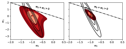
Therefore, from the above discussion it becomes clear that the ideal avenue that cosmologists need to follow towards understanding the nature of the cosmic acceleration is to use future high quality $H(z)$ data to measure the dark energy equation of state and the matter content of the Universe. This issue is discussed in section IV. In particular, Monte-Carlo predictions show that for the realistic future expectations of $\sim 100$ $H(z)$ measurements, we predict that the present FoM of the non-flat $\Lambda$CDM model is increased by a factor of two, while in the case of the CPL parametrization we find three-fold increase of the corresponding FoM. As an example, we provide in the right panel of Fig. 9 the contours of one simulation of 100 $H(z)$ measurements for the CPL model in the $w_{0}-w_{1}$ plane (red-scale contours) For comparison we plot the corresponding contours (black curves) of the Union 2.1 set of 580 SN Ia of Suzuki et al. Suzuki:2011hu . Obviously, in the case of SNIa data we observe that the parameters $w_{0}$ and $w_{1}$ are degenerate. This seems to hold also for the JLA data Betoule14 . However, our Monte Carlo analysis suggests that with the aid of only $\sim 100$ future $H(z)$ measurements in the redshift range $0<z<2.4$, we will be able to put strong constraints on $w_{0}$ as well as to reduce significantly the $w_{1}$ uncertainty and thus testing the evolution of the DE equation of state parameter. We argue that having the future $H(z)$ data available we will be in a position to use these data combined with SNIa and other probes to whittle away the available parameter space for the contender dark matter/energy scenarios and hopefully to settle on a single viable model.

In a nutshell, we would like to make clear that with the present analysis we don’t want to compete SNIa or other cosmological probes. The aim of our article is to investigate the power of direct measurements of the cosmic expansion, towards constraining the dark energy models and to provide the appropriate observational framework for future work.

VI Conclusions

We investigated the performance of the latest expansion data, the so called $H(z)$ measurements, towards constraining the dark energy models. In the context of $H(z)$ data aimed at testing the various forms of dark energy, it is important to minimize the amount of priors needed to successfully complete such a task. One such prior is the Hubble constant and its measurement at the $\sim 1\%$ accuracy level has been proposed as a necessary step for constraining the dark energy models. However, it is well known that the best choice of the value of $H_{0}$ is rather uncertain, namely it has been found a $\sim 3.1\sigma$ tension between the value provided by the Planck team (see Planck16 ) and the results obtained by the SNIa project (Riess et al. Riess16 ). In order to circumvent this problem we implemented in the first part of our work a statistical method which is not affected by the value of $H_{0}$. Based on the latter approach we found that the $H(z)$ data do not rule out the possibility of either non-flat models or dynamical dark energy cosmological models.

Then we performed a joint likelihood analysis using the $H(z)$ and the SNIa data, thereby putting tight constraints on the cosmological parameters, namely $\Omega_{m0}-\Omega_{\Lambda 0}$ (non-flat $\Lambda$CDM model) and $\Omega_{m0}-w$ (wCDM model). Furthermore, using the CPL parametrization we found that the $w_{0}-w_{1}$ parameter space provided by the $H(z)$/SNIa joint analysis is in a very good agreement with that of Planck 2015, which confirms that the present analysis with the $H(z)$ and SNIa probes correctly captures the expansion of the Universe as found by the team of Planck.

Finally, we performed sets of Monte Carlo simulations in order to quantify the ability of the $H(z)$ data to provide strong constraints on the model parameters. The Monte Carlo approach showed substantial improvement of the constraints, when increasing the sample to $\sim 100$ $H(z)$ measurements. Such a target can be achieved in the future, especially in the light of the next generation of surveys.

Appendix

With the aid of the our statistical method (see section II) we calculate the new chi-square estimator that is relevant in the case of the covariance matrix. If the data are correlated then the chi-square estimator is written as:

$$\chi^{2}_{H}={\bf V}{\bf C}^{-1}_{\rm cov}{\bf V}^{T},$$ (12)

where ${\bf C}^{-1}_{\rm cov}$ is the inverse of the covariance matrix Yu17 and

$${\bf V}=\{H_{\rm obs}(z_{1})-H_{M}(z_{1},\phi^{\mu}),...,H_{\rm obs}(z_{N})-H_{M}(z_{N},\phi^{\mu})\}$$

or using Eq.(2) we have

$${\bf V}=\{H_{\rm obs}(z_{1})-H_{0}E(z_{1},\phi^{\mu+1}),..,H_{\rm obs}(z_{N}-H_{0}E(z_{N},\phi^{\mu+1})\}$$

Inserting the latter vector into Eq. (12) we obtain after some algebra

$$\chi^{2}_{H}=AH_{0}^{2}-2BH_{0}+\Gamma$$

and thus following the procedure of section II the functional form of the marginalized ${\tilde{\chi}}^{2}_{H}$ estimator boils down to that of Eq.(8). Notice, that the quantities $A,B,\Gamma$ are given by

$$A={\bf E}{\bf C}^{-1}_{\rm cov}{\bf E}^{T},$$

$$B=\frac{1}{2}\left({\bf E}{\bf C}^{-1}_{\rm cov}{\bf H}_{\rm obs}^{T}+{\bf H}_{\rm obs}{\bf C}^{-1}_{\rm cov}{\bf E}^{T}\right)\\$$

$$\Gamma={\bf H}_{\rm obs}{\bf C}^{-1}_{\rm obs}{\bf H}_{\rm obs}^{T}$$

with

$${\bf E}=\{E(z_{1},\phi^{\mu+1}),...,E(z_{N},\phi^{\mu+1})\}$$

and

$${\bf H}_{\rm obs}=\{H_{\rm obs}(z_{1}),..,H_{\rm obs}(z_{N})\}\;.$$

References

- (1) Planck Collaboration et al., A & A, 594, A13, (2016)
- (2) Amendola, L., Tsujikawa, S., Dark Energy: Theory and Observations Hardcover, Campbrige 2010
- (3) Durrer R. & Maartens, R., ”Dark Energy: Observational & Theoretical Approaches”, ed. P Ruiz-Lapuente (Cambridge UP, 2010), pp48 - 91, (2010) [arXiv:0811.4132v1] (
- (4) Kim, A. G., et al., Astroparticle Physics, 63, 2 (2015)
- (5) N. Suzuki, D. Rubin, C. Lidman, G. Aldering, R. Amanullah, K. Barbary, L. F. Barrientos and J. Botyanszki et al., Astrophys. J. 746, 85 (2012)
- (6) M. Betoule, R. Kessler, J. Guy, J. Mosher, D. Hardin,et al. Astron. & Astrophys., A22, 568 (2014)
- (7) Amati et al.. Astroph. J., 390, 81 (2002); Ghirlanda, Ghisellini & Firmani New J. Phys., 8, 123 (2006); Basilakos & Perivolaropoulos Mon. Not. R. Soc., 391, 4112008 (2008); Wang, F. Y., Dai, Z. G. & Liang, E. W., New Astronomy Reviews, 67, 1 (2015)
- (8) Plionis, M. et al., Mon. Not. R. Astron. Soc. 416, 2981 (2011)
- (9) Chavez R., et al., Mon. Not. R. Astron. Soc., 462, 2431 (2016)
- (10) Yu H., Ratra B., &, Wang Fa-Yin, [arXiv:1711.0343] (2017)
- (11) Blake, C. et al., Mon. Not. R. Soc, , 418, 1707 (2011)
- (12) Alam, S., et al., Mon. Not. R. Soc, , 470, 2617 (2017)
- (13) Calabrese E., Battaglia N. & Spergel, D. N., Clas. Q. Grav., 33, 165004 (2016)
- (14) Nesseris S., Pantazis G. & Perivolaropoulos, L., Phys. Rev. D., 96, 023542 (2017); Basilakos S. & Nesseris S., Phys. Rev. D., 96, 063517 (2017)
- (15) Wang, Y. & Tegmark, M., Phys. Rev. D., 71, 103513 (2005)
- (16) Shapiro C. & Turner, M. S. , Astroph. J. , 649 (2006)
- (17) Samushia, L., & Ratra. B, Astroph. J. Lett., 650.1 (2006): L5.
- (18) Farooq, O., & Ratra B., Astroph. J. Lett., 766, 1 (2013)
- (19) Chimento, Luis P., Richarte, Martin G., & Garcia I. E. S., Phys. Rev. D 88, 087301 (2013)
- Ferreira et al. (2013) Ferreira P. C., Pavón D., & Carvalho J. C., Phys. Rev. D, 88, 083503 (2013)
- Capozziello et al. (2014) Capozziello, S., Farooq, O., Luongo, O., & Ratra, B., Phys. Rev. D, 90, 044016 (2014)
- (22) Gruber, C., & Luongo, O., Phys. Rev. D 89, 103506 (2014)
- Forte (2014) Forte M., Gen. Rel. Grav., 46, 1811 (2014)
- Dankiewicz et al. (2014) Dankiewicz, T., Dabrowski, M. P., Martins, C. J. A. P., & Vielzeuf, P. E., Phys. Rev. D, 89, 083514 (2014)
- Cai et al. (2014) Cai, R.-G., Guo., Z.-K., & Yang, T., Phys. Rev. D, 93, 43517 (2015)
- (26) Melia F., & McClintock, T., M., Astron. J., 150, 6 (2015)
- Chen et al. (2016a) Chen, Y., Kumar, S., & Ratra, B., Astrophys. J, 835, 86 (2017)
- Mukherjee & Banerjee (2016) Mukherjee, A. & Banerjee, N. 2016, Phys. Rev. D, 93, 043002 [arXiv:1601.05172]
- (29) Farooq O., Madiyar F. R., Crandall S., & Ratra B., Astrophys. J., 835, 26 (2017)
- (30) Nunes,R. C., Pan, S., & Saridakis E., JCAP, 1608, 11 (2016)
- (31) Magana, J. et al, arxiv preprint, [arXiv:1706.09848v1], (2017)
- (32) Nunes, R. F et al, [arXiv:1610.07518] (2017)
- (33) Pier-Stefano, C., Huterer, D. & Melchiorri, A. , Phys. Rev. 75, 062001 (2007)
- (34) Jimenez, R., and Loeb, A., Astrophys. J., 37 (2002)
- (35) Riess A. G., et al., Astrophys. J, 826, 56 (2016)
- (36) L. Taddei and L. Amendola, JCAP, 02, 001 (2015)
- (37) Basilakos, S., & Nesseris, S., Phys. Rev. D 94.12 (2016).
- (38) M. S. Turner and M. White, Phys. Rev. D 56, R4439 (1997); T. Chiba, N. Sugiyama, and T. Nakamura, Mon. Not. Roy. Astron. Soc. 289, L5 (1997); J. A. S. Lima and J. S. Alcaniz, Astron. Astrophys. 357, 393 (2000);, Astrophys. J. 566, 15 (2002)
- (39) E. V. Linder, Phys. Rev. Lett., 90(9), (2003)
- (40) M. Chevallier, D. Polarski Int. J. Mod. Phys., D10(2) (2001)
- (41) J. F. Jesus, T. M. Gregorio and F. Andrade-Oliveira, [arXiv:1709.0064]
- (42) Riess A. G., et al., Astrophys. J., 730, 119 (2011); Erratum: Astrophys. J. 732, 129 (2011)
- (43) Simon, J., Licia Verde, & Raul Jimenez, Physical Review D, 71.12 (2005)
- (44) Moresco, M., et al. , Jour. Cosmology and Astrop. Physics, 08 (2012)
- (45) Stern, D., et al., The Astroph. Jour. Suppl. Series 188 (2010)
- (46) Blake, C., et al., Mon. Not. Royal Astron. Soc., 425 (2012)
- (47) Zhang, C., et al., Research in Astron. & Astroph., 14 (2014)
- (48) Font-Ribera, A., et al., Jour. Cosmo. & Astrop. Phys., 05 (2014)
- (49) Delubac, T., et al., Astron. & Astroph. 574 (2015)
- (50) Moresco, M., Month. Not. of the Royal Astron. Soc.: Lett. 450 (2015)
- (51) Moresco, Michele, et al., Jour. Cosmo. & Astrop. Phys., 05 (2016)
- (52) Bassett, B. A., Parkinson D., &. Nichol, R. C. The Astroph. Jour. Lett. 626.1 (2005): L1.
- (53) Rubin, D. et al, [arXiv:1507.01602v4] (2017)
- (54) S. Nesseris & L. Perivolaropoulos, Phys. Rev. D., 72, 123519