On the Stability of Einstein Universe in $f(R,T,R_{\mu\nu}T^{\mu\nu})$ Gravity

Abstract

This paper investigates the existence and stability of Einstein universe in the context of $f(R,T,Q)$ gravity, where $Q=R_{\mu\nu}T^{\mu\nu}$. Considering linear homogeneous perturbations around scale factor and energy density, we formulate static as well as perturbed field equations. We parameterize the stability regions corresponding to conserved as well as non-conserved energy-momentum tensor using linear equation of state parameter for particular models of this gravity. The graphical analysis concludes that for a suitable choice of parameters, the stable regions of the Einstein universe are obtained.

Keywords: Stability analysis; Einstein universe; Modified gravity.
PACS: 04.25.Nx; 04.40.Dg; 04.50.Kd.

1 Introduction

The fact that our universe is going through an accelerated expansion is one of the most spectacular discoveries of modern cosmology. This motivated many researchers to investigate the reason behind the phase of accelerated expansion. It is claimed that dark energy (DE) having large negative pressure with repulsive effects is responsible for the current expanding behavior of the universe. In order to explore the mysterious nature of DE, several proposals have been studied including modified theories of gravity as the inspiring approach. These modified theories are the generalizations of the Einstein-Hilbert action like $f(R)$ ($R$ indicates Ricci scalar) [1], $f(\mathcal{G})$ ($\mathcal{G}$ represents Gauss-Bonnet invariant term) [2], $f(\mathcal{T})$ ($\mathcal{T}$ shows torsion) [3], $f(R,T)$ ($T$ describes the trace of energy-momentum tensor (EMT)) [4], $f(\mathcal{G},T)$ [5] and $f(R,T,Q)$ ($Q$ is the contraction of Ricci tensor and EMT) gravity [6].

The $f(R,T,Q)$ gravity, an extension of $f(R,T)$ gravity, has gained much attention due to its strong non-minimal coupling between gravity and matter fields. Odintsov and S$\acute{a}$ez-G$\acute{o}$mes [7] explored matter instability, $\Lambda$CDM model and de Sitter solutions in this modified theory. Sharif and Zubair investigated the validity of thermodynamical laws [8] and derived the energy conditions [9] for two different models of this gravity. The isotropic as well as anisotropic physical behavior of compact relativistic objects are also discussed in this gravity [10]. Baffou et al. [11] explored the stability analysis of this modified theory corresponding to de Sitter and power-law solutions using perturbation approach and found stable solutions. Recently, Yousaf et al. [12] studied the stability of cylindrical system for a particular $f(R,T,Q)$ model and examined the instability constraints at Newtonian and post-Newtonian limits.

The emergent universe scenario (which helps to resolve the issue of big-bang singularity) is based on the existence as well as stability of the Einstein universe (EU) against all kinds of perturbations. In general relativity (GR), the idea of this emergent universe is not proved successful due to unstable EU against homogenous perturbations. The existence and stability of EU in modified theories is of great importance. The stability of EU has been checked in brane-world models, GR with small inhomogeneous vector and tensor perturbations, GR with variable pressure, Einstein-Cartan theory, loop quantum cosmology etc [13]. Böhmer et al. [14] examined the stability of EU against linear perturbations in $f(R)$ theory and found the existence of stable regions for particular models of this theory. Goswami et al. [15] observed the existence and stable modes of EU in the context of fourth-order modified theory. Goheer and his collaborators [16] found stable solutions of EU corresponding to power-law model in $f(R)$ gravity. Böhmer and Lobo [17] discussed existence as well as stability of EU in $f(\mathcal{G})$ gravity and obtained stable states for different values of equation of state (EoS) parameter.

Carneiro and Tavakol [18] investigated the existence of EU and its stability under the effects of vacuum energy corresponding to conformally invariant fields. Seahra and Böhmer [19] showed that stable EU solutions exist in $f(R)$ models only for perfect fluid with linear EoS whereas they remain unstable against inhomogeneous perturbations. Canonico and Parisi [20] studied the stability of EU in Hořava-Lifshitz gravity under some certain conditions and similar analysis is performed in the framework of massive gravity [21]. Böhmer et al. [22] examined the stability of EU in hybrid metric-Palatini gravity using homogeneous as well as inhomogeneous linear perturbations and found the existence of large class of stable solutions. Li et al. [23] analyzed the stable modes for open as well as closed universe by considering homogeneous perturbations in teleparallel modified theory.

Huang et al. [24] found stable EU solutions against anisotropic and homogenous perturbations in the background of Jordan-Brans-Dicke theory. The same authors [25] also established the unstable solutions for open universe and stable regions for closed universe in Gauss-Bonnet gravity. Böhmer et al. [26] examined the stability modes against homogeneous as well as inhomogeneous perturbations in scalar-fluid theories and obtained stable and unstable results corresponding to inhomogeneous and homogeneous perturbations, respectively. Darabi and his collaborators [27] studied the existence of EU and its stability in the framework of Lyra geometry using scalar, vector and tensor perturbations with suitable choice of parameters. Shabani and Ziaie [28] discussed the stable solutions of EU in $f(R,T)$ gravity which were unstable in $f(R)$ gravity. Sharif and Ikram [29] investigated the stability of EU against linear homogeneous perturbations in $f(\mathcal{G},T)$ gravity. They found that stable EU solutions exist and their results reduce to $f(\mathcal{G})$ gravity in the absence of matter-curvature coupling.

In this paper, we explore the stability of EU by applying homogeneous linear perturbations in the framework of $f(R,T,Q)$ gravity. This study would help to investigate the effects of strong non-minimal coupling of matter and geometry on the stability of EU. The format of this paper is as follows. In the next section, we formulate the corresponding field equations of this theory. Section 3 deals with the stability of EU for both conserved and non-conserved EMT. In the last section, we summarize our concluding remarks.

2 Formalism of $f(R,T,Q)$ Gravity

The action for $f(R,T,Q)$ gravity is defined as [6]

$$S=\frac{1}{2\kappa^{2}}\int d^{4}x\sqrt{-g}[f(R,T,Q)+\mathcal{L}_{m}],$$ (1)

where $\kappa^{2}$ and $\mathcal{L}_{m}$ represent coupling constant and matter Lagrangian density, respectively. The EMT corresponding to $\mathcal{L}_{m}$ is given by [30]

$$T^{\mu\nu}=\frac{2}{\sqrt{-g}}\frac{\delta(\sqrt{-g}\mathcal{L}_{m})}{\delta g_{\mu\nu}}=g^{\mu\nu}\mathcal{L}_{m}+\frac{2\delta\mathcal{L}_{m}}{\delta g_{\mu\nu}}.$$ (2)

Varying the action (1) with respect to $g_{\mu\nu}$, we obtain the field equations

$$G_{\mu\nu}=R_{\mu\nu}-\frac{1}{2}Rg_{\mu\nu}=T_{\mu\nu}^{eff},$$ (3)

where the effective EMT is of the form

$$T_{\mu\nu}^{eff} = \frac{1}{f_{R}-f_{Q}\mathcal{L}_{m}}\left[(1+f_{T}+\frac{1}{2}Rf_{Q})T_{\mu\nu}+\left\{\frac{1}{2}(f-Rf_{R})-\mathcal{L}_{m}f_{T}\right.\right.$$ (4)

$$- \left.\left.\frac{1}{2}\nabla_{\alpha}\nabla_{\beta}(f_{Q}T^{\alpha\beta})\right\}g_{\mu\nu}-(g_{\mu\nu}\Box-\nabla_{\mu}\nabla_{\nu})f_{R}+\nabla_{\alpha}\nabla_{(\mu}[T_{\nu)}^{\alpha}f_{Q}]\right.$$

$$- \left.\frac{1}{2}\Box(f_{Q}T_{\mu\nu})-2f_{Q}R_{\alpha(\mu}T_{\nu)}^{\alpha}+2(f_{T}g^{\alpha\beta}+f_{Q}R^{\alpha\beta})\frac{\partial^{2}\mathcal{L}_{m}}{\partial g^{\mu\nu}\partial g^{\alpha\beta}}\right].$$

The subscripts of generic function $f$ show derivative with respect to $R,~{}Q$ and $T$. The covariant divergence of field equation (4) is given by

$$\nabla^{\mu}T_{\mu\nu}^{eff} = \frac{2}{2(1+f_{T})+Rf_{Q}}\left[\nabla_{\mu}(f_{Q}R^{\sigma\mu}T_{\sigma\nu})+\nabla_{\nu}(\mathcal{L}_{m}f_{T})-G_{\mu\nu}\nabla_{\mu}(f_{Q}\mathcal{L}_{m})\right.$$ (5)

$$- \left.\frac{1}{2}(f_{Q}R_{\alpha\beta}+f_{T}g_{\alpha\beta})\nabla_{\nu}T^{\alpha\beta}-\frac{1}{2}[\nabla^{\mu}(Rf_{Q})+2\nabla^{\mu}f_{T}]T_{\mu\nu}\right].$$

The line element for closed FRW universe model is

$$ds^{2}=dt^{2}-a^{2}(t)\left(\frac{1}{1-r^{2}}dr^{2}+r^{2}(d\theta^{2}+\sin^{2}\theta d\phi^{2})\right),$$ (6)

where $a(t)$ represents the scale factor. The EMT for perfect fluid is

$$T_{\mu\nu}=(\rho+p)u_{\mu}u_{\nu}-pg_{\mu\nu},$$ (7)

where $\rho,~{}p$ and $u_{\mu}$ indicate energy density, pressure and four velocity, respectively. As we are interested to find the stable region of EU with perfect fluid, so matter Lagrangian can be taken as $\mathcal{L}_{m}=-p$ [4]. In closed FRW universe background, the field equations of this modified theory corresponding to matter Lagrangian are obtained as

$$\frac{3}{a^{2}}(1+\dot{a}^{2}) = \frac{1}{f_{R}+pf_{Q}}\left[\kappa^{2}\rho+(\rho+p)f_{T}+3\left(\frac{a\ddot{a}+\dot{a}^{2}+1}{a^{2}}\right)f_{R}+\frac{1}{2}\right.$$ (8)

$$\times \left.f(R,T,Q)-3\frac{\dot{a}}{a}\partial_{t}f_{R}-\frac{3}{2}\left(\frac{4\dot{a}^{2}-a\ddot{a}+2}{a^{2}}\right)\rho f_{Q}-\frac{3}{2}\right.$$

$$\times \left.\left(\frac{a\ddot{a}+2\dot{a}^{2}}{a^{2}}\right)pf_{Q}+\frac{3\dot{a}}{2a}\partial_{t}[(p-\rho)f_{Q}]\right],$$

$$-2a\ddot{a}-(1+\dot{a}^{2}) = \frac{1}{f_{R}+pf_{Q}}\left[\kappa^{2}a^{2}p-\frac{a^{2}}{2}f(R,T,Q)-3(a\ddot{a}+\dot{a}^{2}+1)f_{R}\right.$$ (9)

$$+ \left.2a\dot{a}\partial_{t}f_{R}+a^{2}\partial_{tt}f_{R}+\frac{1}{2}\left(\frac{4\dot{a}^{2}-a\ddot{a}+2}{a^{2}}\right)pf_{Q}+\frac{1}{2}(a\ddot{a}\right.$$

$$+ \left.2\dot{a}^{2})\rho f_{Q}+2a\dot{a}\partial_{t}[(p+\rho)f_{Q}]+\frac{a^{2}}{2}\partial_{tt}[(\rho-p)f_{Q}]\right],$$

where dot shows derivative with respect to time. The conservation equation (5) with perfect fluid becomes

$$\dot{\rho}+3\frac{\dot{a}}{a}(\rho+p) = \frac{1}{2\kappa^{2}+3(f_{T}-\frac{2\dot{a}^{2}+a\ddot{a}}{a^{2}}f_{Q})}\left[\left\{3\frac{\dot{a}}{a^{3}}\left(a\ddot{a}-4\dot{a}^{2}\right)(\rho+p)\right.\right.$$ (10)

$$- \left.\left.3(\frac{a\ddot{a}-\dot{a}^{2}}{a^{2}})\partial_{t}p\right\}f_{Q}-2(\rho+p)\partial_{t}f_{T}+6(\frac{\dot{a}}{a})^{2}(\rho+p)\right.$$

$$\times \left.\partial_{t}f_{Q}+\partial_{t}pf_{T}\right].$$

3 Stability Analysis of Einstein Universe

In this section, we consider linear homogeneous perturbations and investigate the stability of EU in $f(R,T,Q)$ gravity. For this purpose, we take $a(t)=a_{0}=constant$ for EU and the corresponding field equations (8) and (9) reduce to

$$\frac{3}{a_{0}^{2}} = \frac{1}{f_{R}+p_{0}f_{Q}}\left[\kappa^{2}\rho_{0}+(\rho_{0}+p_{0})f_{T}+\frac{1}{2}f(R_{0},T_{0},Q_{0})+\frac{3}{a_{0}^{2}}f_{R}-\frac{3}{a_{0}^{2}}\rho_{0}f_{Q}\right],$$

$$-\frac{1}{a_{0}^{2}} = \frac{1}{f_{R}+p_{0}f_{Q}}\left[\kappa^{2}p_{0}-\frac{1}{2}f(R_{0},T_{0},Q_{0})-\frac{3}{a_{0}^{2}}f_{R}+\partial_{tt}f_{R}+\frac{1}{a_{0}^{2}}p_{0}f_{Q}\right.$$ (12)

$$+ \left.\frac{1}{2}\partial_{tt}[(\rho_{0}-p_{0})f_{Q}]\right],$$

where $R_{0}=R(a_{0})=-\frac{6}{a_{0}^{2}}$, $T_{0}=\rho_{0}-3p_{0}$ and $Q_{0}=6\frac{p_{0}}{a_{0}^{2}}$. Here $\rho_{0}$ and $p_{0}$ denote the unperturbed energy density and pressure, respectively. In order to examine the stability regions, we consider linear EoS defined as $p(t)=\omega\rho(t)$ ($\omega$ is the EoS parameter) and introduce the expressions for linear perturbations in scale factor and energy density depending only on time as follows

$$a(t)=a_{0}+a_{0}\delta a(t),\quad\rho(t)=\rho_{0}+\rho_{0}\delta\rho(t),$$ (13)

where $\delta a(t)$ and $\delta\rho(t)$ express the perturbed scale factor and energy density, respectively. We assume that $f(R,T,Q)$ is analytic and by applying Taylor series expansion for three variables upto first order, this turns out to be

$$f(R,T,Q) = f(R_{0},T_{0},Q_{0})+f_{R}(R_{0},T_{0},Q_{0})\delta R+f_{T}(R_{0},T_{0},Q_{0})\delta T$$ (14)

$$+ f_{Q}(R_{0},T_{0},Q_{0})\delta Q.$$

Using linear EoS, $\delta R$, $\delta T$ and $\delta Q$ become

$$\delta R=-6(\delta\ddot{a}-2\frac{\delta a}{a_{0}^{2}}),\quad\delta T=T_{0}\delta\rho_{0},\quad\delta Q=3\rho_{0}[(\omega-1)\delta\ddot{a}-4\frac{\omega}{a_{0}^{2}}\delta a+2\frac{\omega}{a_{0}^{2}}\delta\rho],$$ (15)

where $\delta\ddot{a}=\frac{d^{2}}{dt^{2}}(\delta a)$. Substituting Eqs.(LABEL:11)-(15) into the field equations (8) and (9), we obtain the linearized perturbed equations as

$$6(f_{R}+\rho_{0}f_{Q})\delta a+a_{0}^{2}\rho_{0}[\kappa^{2}+(1+\omega)f_{T}+\frac{1}{2}(1-3\omega)f_{T}-\frac{3}{a_{0}^{2}}f_{Q}]\delta\rho=0,$$ (17)

$$2(f_{R}+\rho_{0}f_{Q})\delta\ddot{a}+\frac{2}{a_{0}^{2}}(\rho_{0}\omega f_{Q}-f_{R})\delta a+\rho_{0}[\kappa^{2}\omega-\frac{1}{2}(1-3\omega)f_{T}-\frac{\omega}{a_{0}^{2}}f_{Q}]\delta\rho$$

$$+ \frac{1}{2}\rho_{0}(1-\omega)f_{Q}\delta\ddot{\rho}=0.$$

These express a direct relation between perturbed scale factor and energy density.

In the following, we discuss the stability of EU for both conserved and non-conserved EMT.

3.1 Stability for Conserved EMT

The conservation law does not hold in $f(R,T,Q)$ theory of gravity like other modified theories having non-minimal coupling between matter and geometry [4, 5]. We assume that this law holds in this gravity for which the right hand side of Eq.(10) becomes zero and we obtain

$$\dot{p}f_{T}-2(\rho+p)\partial_{t}f_{T}+\frac{3}{a^{2}}\left[\frac{\dot{a}}{a}(a\ddot{a}-4\dot{a}^{2})(\rho+p)-(a\ddot{a}-\dot{a}^{2})\dot{p}\right]f_{Q}$$ (18)

$$+ 6(\frac{\dot{a}}{a})^{2}(\rho+p)\partial_{t}f_{Q}=0.$$

From the standard conservation equation, we obtain the relation defined by

$$\delta\dot{\rho}(t)=-3(1+\omega)\delta\dot{a}(t).$$ (19)

In order to have the perturbed field equation in the form of perturbed scale factor, we eliminate $\delta\rho$ from Eqs.(LABEL:16) and (17) and then substitute Eq.(19) in the resulting equation, it follows that

$$\left[\frac{2}{a_{0}^{2}}(f_{R}-\omega\rho_{0}f_{Q})\left[a_{0}^{2}\rho_{0}\left\{\kappa^{2}+(1+\omega)f_{T}+\frac{1}{2}(1-3\omega)f_{T}-\frac{3}{a_{0}^{2}}f_{Q}\right\}\right]+6\right.$$

$$\times \left.\rho_{0}(f_{R}+\rho_{0}f_{Q})\left\{\kappa^{2}\omega-\frac{1}{2}(1-3\omega)f_{T}-\frac{\omega}{a_{0}^{2}}f_{Q}\right\}\right]\delta a+\left[a_{0}^{2}\rho_{0}\left\{\kappa^{2}+(1+\omega)\right.\right.$$

$$\times \left.\left.f_{T}+\frac{1}{2}(1-3\omega)f_{T}-\frac{3}{a_{0}^{2}}f_{Q}\right\}\left\{\frac{3}{2}\rho_{0}(1-\omega^{2})f_{Q}-2(f_{R}+\rho_{0}f_{Q})\right\}\right]\delta\ddot{a}=0.$$

To determine the expression for $a_{0}^{2}$, adding Eqs.(LABEL:11) and (12) which leads to

$$a_{0}^{2}=\frac{2f_{R}+\rho_{0}(3+\omega)f_{Q}}{\rho_{0}(1+\omega)(\kappa^{2}+f_{T})}.$$ (21)

Using this value in Eq.(LABEL:20), the perturbed field equation takes the form

$$\left[2(f_{R}-\omega\rho_{0}f_{Q})\left[\rho_{0}\left\{\kappa^{2}+(1+\omega)f_{T}-\left(\frac{3\rho_{0}(1+\omega)(\kappa^{2}+f_{T})}{2f_{R}+\rho_{0}(3+\omega)f_{Q}}\right)f_{Q}\right.\right.\right.$$ (22)

$$+ \left.\left.\left.\frac{1}{2}(1-3\omega)f_{T}\right\}\right]+6\rho_{0}(f_{R}+\rho_{0}f_{Q})\left\{\kappa^{2}\omega-\left(\frac{\omega\rho_{0}(1+\omega)(\kappa^{2}+f_{T})}{2f_{R}+\rho_{0}(3+\omega)f_{Q}}\right)\right.\right.$$

$$\times \left.\left.f_{Q}-\frac{1}{2}(1-3\omega)f_{T}\right\}\right]\delta a+\left[\rho_{0}\left(\frac{2f_{R}+\rho_{0}(3+\omega)f_{Q}}{\rho_{0}(1+\omega)(\kappa^{2}+f_{T})}\right)\left\{\kappa^{2}+(1+\omega)\right.\right.$$

$$\times \left.\left.f_{T}+\frac{1}{2}(1-3\omega)f_{T}-\left(\frac{3\rho_{0}(1+\omega)(\kappa^{2}+f_{T})}{2f_{R}+\rho_{0}(3+\omega)f_{Q}}\right)f_{Q}\right\}\left\{\frac{3}{2}\rho_{0}(1-\omega^{2})f_{Q}\right.\right.$$

$$- \left.\left.2(f_{R}+\rho_{0}f_{Q})\right\}\right]\delta\ddot{a}=0.$$

As in other modified theories, we also have fourth-order perturbed field equations in this theory. However, it vanishes due to the presence of $Q$ term (product of Ricci tensor and EMT) as we are assuming only the first-order linear terms. Thus we obtain a second-order perturbation equation about $a(t)$ in this modified theory. In the GR limit, i.e., for $f_{R}=1$ and $f_{T}=0=f_{Q}$, Eq.(22) reduces to the desired form given by

$$2\delta\ddot{a}-\rho_{0}(1+\omega)(1+3\omega)\delta a=0.$$

The solution of Eq.(22) is helpful to examine the stability modes of EU but due to a complicated nature of this theory, it would be a difficult task. For this purpose, we consider a specific form of $f(R,T,Q)$ gravity defined as follows [7]

$$f(R,T,Q)=R+f(T)+g(Q),$$ (23)

where $f(T)$ and $g(Q)$ are the generic functions of $T$ and $Q$, respectively. We assume that the conservation law holds for this model. Consequently, the resulting second-order differential equation is obtained using this particular form in Eq.(18) as

$$\omega f^{\prime}(T)-2(1+\omega)Tf^{\prime\prime}(T)=0,$$

where prime shows derivative with respect to $x(x=R$, or $T$, or $Q)$. The solution of this equation is

$$f(T)=\frac{c_{1}T(1+\omega)(2T(1+\omega))^{\frac{\omega}{2(1+\omega)}}}{2+3\omega}+c_{2},$$ (24)

where $c_{1}$ and $c_{2}$ are integration constants.

It is mentioned here that the conservation law holds only for this unique expression of $f(T)$ in the model (23). Now substituting the values from Eqs.(23) and (24) in (22), the resulting differential equation takes the form

$$\left[6\{\Delta_{1}+\Delta_{2}\Delta_{3}+2\Delta_{3}^{2}\Delta_{4}\}-3g^{\prime}(Q)\{2\Delta_{5}+\Delta_{3}\Delta_{6}-\Delta_{3}^{2}\Delta_{7}\}\right]\delta a$$ (25)

$$- [(\Delta_{8}+\Delta_{9})g^{\prime}(Q)+2\Delta_{3}\Delta_{10}]\delta\ddot{a}=0,$$

where $\Delta_{i}$’s $(i=1,2,3,...,10)$ are

$$\Delta_{1} = \frac{\rho_{0}\kappa^{4}}{3}(1+4\omega+3\omega^{2}),$$

$$\Delta_{2} = \rho_{0}\kappa^{2}\left(1+\omega(10+7\omega)+2\rho_{0}\omega(1+3\omega+\omega^{2})\right),$$

$$\Delta_{3} = \frac{c_{1}}{2}\left(2\rho_{0}(1+\omega)(1-3\omega)\right)^{\frac{\omega}{2(1+\omega)}},$$

$$\Delta_{4} = \rho_{0}\omega(2+\omega+\rho_{0}(1+\omega+\omega^{2})),$$

$$\Delta_{5} = \rho_{0}^{2}\omega\kappa^{4}(1+4\omega+3\omega^{2}),$$

$$\Delta_{6} = \rho_{0}^{2}\kappa^{2}(8\omega(1+\omega)+3(1-\omega^{4})),$$

$$\Delta_{7} = \rho_{0}^{2}(\kappa^{2}\omega^{2}(1+3\omega)-3(1+2\omega)+3\omega^{3}(2+\omega)),$$

$$\Delta_{8} = \kappa^{2}\left(2(3+\omega)+\rho_{0}(1-4\omega+3\omega^{2})\right),$$

$$\Delta_{9} = 9-\omega^{2}+\frac{\rho_{0}}{2}(9-13\omega+7\omega^{2}-3\omega^{3}),$$

$$\Delta_{10} = \frac{2\kappa^{2}}{\Delta_{3}}+(3-\omega).$$

The solution of Eq.(25) is given by

$$\delta a(t)=b_{1}e^{\Omega t}+b_{2}e^{-\Omega t}.$$

Here $b_{1}$ and $b_{2}$ are constants of integration and the parameter $\Omega$ represents the frequency of small perturbation which is of the form

$$\Omega^{2}=\frac{6(\Delta_{1}+\Delta_{2}\Delta_{3}+2\Delta_{3}^{2}\Delta_{4})-3g^{\prime}(Q)(2\Delta_{5}+\Delta_{3}\Delta_{6}-\Delta_{3}^{2}\Delta_{7})}{(\Delta_{8}+\Delta_{9})g^{\prime}(Q)+2\Delta_{3}\Delta_{10}}.$$ (26)

In order to avoid the exponential increase in $\delta a(t)$ or collapse, the parameter $\Omega^{2}<0$, which leads to the stability of EU. In general relativistic limit, this frequency is given by

$$\Omega^{2}=\frac{1}{2}\kappa^{2}\rho_{0}(1+\omega)(1+3\omega),$$

which shows the stable solution in the range $-1<\omega<-\frac{1}{3}$ [17].

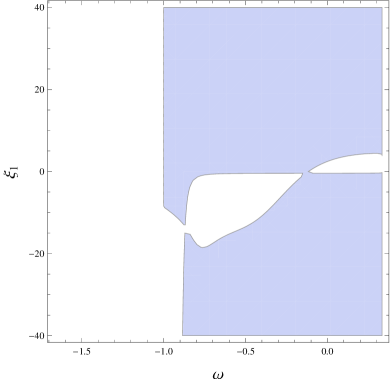
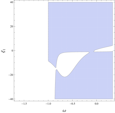
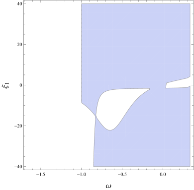
Figure 1: Plots of stable regions in $(\omega,\xi_{1})$ space for $\Omega^{2}$ with $c_{1}=1$ (left), $c_{1}=4$ (right) and $c_{1}=7$ (below).

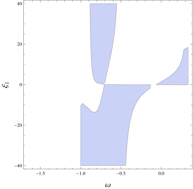
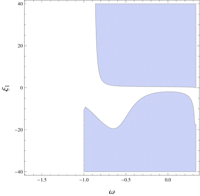
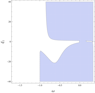
Figure 2: Plots of stable regions in $(\omega,\xi_{1})$ space for $\Omega^{2}$ with $c_{1}=-1$ (left), $c_{1}=-4$ (right) and $c_{1}=-7$ (below).

To analyze the graphical behavior of stable modes of EU, we take $\kappa^{2}=1$, $\rho_{0}=0.3$ [31] and $g^{\prime}(Q)=\xi_{1}$ as a new parameter. Figure 1 shows the existence of stable EU for $\Omega^{2}$ under linear perturbations corresponding to different positive values of $c_{1}$. It is observed that the stable EU exists for all values of $\omega\geq-1$ and these stability regions are becoming more smooth with increasing value of integration constant $c_{1}$. The graphical behavior in Figure 2 describes the EU and its stability for negative values of $c_{1}$. It is found that for $c_{1}=-1$, the stable modes exist in the range of $-1<\omega<\frac{1}{3}$ and with decreasing value of $c_{1}$, the graphs show more stable regions towards positive values of EoS parameter.

3.2 Stability for Non-Conserved EMT

In this section, we discuss the stability when EMT is not conserved. Here we consider another specific model which consists of linear form of $R$ and generic function $f(Q)$ defined as follows [7]

$$f(R,T,Q)=\alpha R+f(Q),$$ (27)

where $\alpha$ is an arbitrary constant. For this model, the perturbed field equations (LABEL:16) and (17) lead to

$$6\left[\alpha+\rho_{0}f^{\prime}(Q)\right]\delta a+a_{0}^{2}\rho_{0}\left[\kappa^{2}-\frac{3}{a_{0}^{2}}f^{\prime}(Q)\right]\delta\rho=0,$$

$$\left[2\alpha+\rho_{0}(\frac{1+3\omega^{2}}{2})f^{\prime}(Q)\right]\delta\ddot{a}+\frac{2}{a_{0}^{2}}\left[\rho_{0}\omega f^{\prime}(Q)-\alpha\right]\delta a$$

$$+ \rho_{0}\omega[\kappa^{2}-\frac{1}{a_{0}^{2}}f^{\prime}(Q)]\delta\rho=0.$$ (29)

These equations represent the relationship between perturbed scale factor and energy density perturbations. The differential equation in perturbed scale factor is obtained by eliminating $\delta\rho$ from Eqs.(3.2) and (29) as

$$a_{0}^{2}\left[2\alpha\kappa^{2}+\left\{\rho_{0}\kappa^{2}(\frac{1+3\omega^{2}}{2})-\frac{6\alpha}{a_{0}^{2}}\right\}f^{\prime}(Q)\right]\delta\ddot{a}+2\left[\left\{\frac{3\alpha}{a_{0}^{2}}(1+\omega)\right.\right.$$ (30)

$$- \left.\left.2\rho_{0}\omega\kappa^{2}\right\}f^{\prime}(Q)-\alpha\kappa^{2}(1+3\omega)\right]\delta a=0.$$

The addition of static field Eqs.(LABEL:11) and (12) corresponding to (27) yields

$$a_{0}^{2}=\frac{2\alpha+\rho_{0}(3+\omega)f^{\prime}(Q)}{\rho_{0}\kappa^{2}(1+\omega)}.$$ (31)

Inserting the value of $a_{0}^{2}$ in Eq.(30), the resulting differential equation is

$$2\kappa^{2}\rho_{0}(1+\omega)\left[\alpha(1+3\omega)+4\omega\rho_{0}f^{\prime}(Q)\right]\delta a-\left[4\alpha^{2}+\alpha\rho_{0}(3\omega^{2}-2\omega\right.$$ (32)

$$+ \left.7)f^{\prime}(Q)\right]\delta\ddot{a}=0,$$

whose solution is obtained as

$$\delta a(t)=a_{1}e^{\bar{\Omega}t}+a_{2}e^{-\bar{\Omega}t},$$ (33)

where $a_{j}$’s $(j=1,2)$ are integration constants and frequency of small perturbation $(\bar{\Omega})$ is of the form

$$\bar{\Omega}^{2}=\frac{2\kappa^{2}\rho_{0}(1+\omega)\left(\alpha(1+3\omega)+4\omega\xi_{2}\right)}{4\alpha^{2}+\alpha(3\omega^{2}-2\omega+7)\xi_{2}},$$

where $\xi_{2}=\rho_{0}f^{\prime}(Q)$.

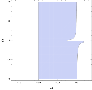
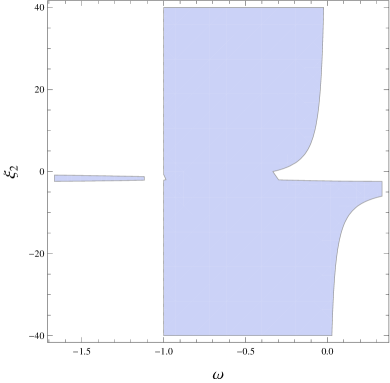
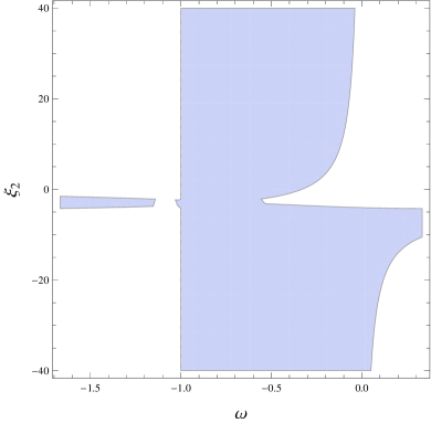
Figure 3: Plots of stable regions in $(\omega,\xi_{2})$ space for $\bar{\Omega}^{2}$ with $\alpha=1$ (left), $\alpha=4$ (right) and $\alpha=7$ (below).

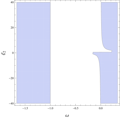
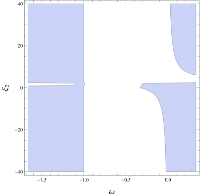
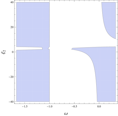
Figure 4: Plots of stable regions in $(\omega,\xi_{2})$ space for $\bar{\Omega}^{2}$ with $\alpha=-1$ (left), $\alpha=-4$ (right) and $\alpha=-7$ (below).

When $\alpha=1$ and $f(Q)=0$, the frequency $\bar{\Omega}^{2}$ regains the result of GR as calculated in the conserved case. The graphical interpretation of stable regions against homogeneous perturbations for different values of arbitrary constant is given in Figures 3 and 4. Figure 3 shows that for $\alpha=1$, the stable regions appear only for negative values of $\omega$ but for greater values of $\alpha$, we obtain some stable region also for positive values of $\omega$. Figure 4 indicates the existence of stable modes of EU for negative values of arbitrary constant and the stability increases with decreasing value of $\alpha$ for both positive as well as negative values of $\omega$.

4 Concluding Remarks

In this paper, we have studied the stability of EU with closed FRW universe model and perfect fluid in the framework of $f(R,T,Q)$ gravity. We have formulated static and perturbed field equations using scalar homogeneous perturbations about energy density and scale factor. These equations are parameterized by linear EoS parameter. The second order perturbed differential equations are constructed whose solutions provide the existence and stability regions of EU for particular $f(R,T,Q)$ models. We have analyzed both conserved as well as non-conserved EMT cases against perturbations scheme. We have found stable results for some positive as well as negative values of model parameters.

We conclude that stable modes of EU exist against homogeneous scalar perturbations for all values of EoS parameter if the model constraints are chosen appropriately in $f(R,T,Q)$ gravity. The stable solutions of EU against vector perturbations are also exist for all equations of state because any initial vector perturbations remain frozen. It is worthwhile to mention here that the range of EoS parameter is greatly enhanced as compared to that in $f(R)$ gravity and more stable regions are found as compared to $f(R,T)$ theory due to the presence of generic function of $Q$. Like all other modified theories, our results also reduce to GR in the absence of dark source terms. It would be interesting to extend our results with the inhomogeneous perturbations around EU which indeed could provide a richer structure for stability analysis of Einstein cosmos in $f(R,T,Q)$ gravity.

References

- [1] Capozziello, S.: Int. J. Mod. Phys. D 483(2002)11.
- [2] Nojiri, S. and Odintsov, S.D.: Phys. Lett. B 631(2005)1.
- [3] Ferraro, R. and Fiorini, F.: Phys. Rev. D 75(2007)084031.
- [4] Harko, T. et al.: Phys. Rev. D 84(2011)024020.
- [5] Sharif, M. and Ikram, A.: Eur. Phys. J. C 76(2016)640.
- [6] Haghani, Z. et al.: Phys. Rev. D 88(2013)044023.
- [7] Odintsov, S.D. and Sez-Gmes, D.: Phys. Lett. B 725(2013)437.
- [8] Sharif, M. and Zubair, M.: J. Phys. Soc. Jpn. 81(2012)114005.
- [9] Sharif, M. and Zubair, M.: J. Cosmol. Astropart. Phys. 12(2013)079.
- [10] Sharif, M. and Waseem, A.: Eur. Phys. J. Plus 131(2016)190; Can. J. Phys. 94(2016)1024.
- [11] Baffou, E.H., Houndjo, M. J. S. and Tossa, J.: Astrophys. Space Sci. 361(2016)376.
- [12] Yousaf, Z., Bhatti, M. Z. and Farwa, U.: Eur. Phys. J. C 77(2017)359.
- [13] Gergely, L.Á. and Maartens, R.: Class. Quantum Grav. 19(2002)213; Barrow, J.D. et al.: Class. Quantum Grav. 20(2003)155; Böhmer, C.G.: Class. Quantum Grav. 36(2004)1039; 21(2004)1119; Mulryne, D.J. et al.: Phys. Rev. D 71(2005)123512.
- [14] Böhmer, C.G., Hollenstein, L. and Lobo, F.S.N.: Phys. Rev. D 76(2007)084005.
- [15] Goswami, R., Goheer, N. and Dunsby, P.K.S.: Phys. Rev. D 78(2008)044011.
- [16] Goheer, N., Goswami, R. and Dunsby, P.K.S.: Class. Quantum Grav. 26(2009)105003.
- [17] Böhmer, C.G. and Lobo, F.S.N.: Phys. Rev. D 79(2009)067504.
- [18] Carneiro, S. and Tavakol, R.: Phys. Rev. D 80(2009)043528.
- [19] Seahra, S.S. and Böhmer, C.G.: Phys. Rev. D 79(2009)064009.
- [20] Canonico, R. and Parisi, L.: Phys. Rev. D 82(2010)064005.
- [21] Parisi, L., Radicella, N. and Vilasi, G.: Phys. Rev. D 86(2012)024035.
- [22] Böhmer, C.G., Lobo, F.S.N. and Tamanini, N.: Phys. Rev. D 88(2013)104019.
- [23] Li, J.T., Lee, C.C. and Geng, C.Q.: Eur. Phys. J. C 73(2013)2315.
- [24] Huang, H., Wu, P. and Yu, H.: Phys. Rev. D 89(2014)103521.
- [25] Huang, H., Wu, P. and Yu, H.: Phys. Rev. D 91(2015)023507.
- [26] Böhmer, C.G., Tamanini, N. and Wright, M.: Phys. Rev. D 92(2015)124067.
- [27] Darabi, F., Heydarzade, Y. and Hajkarim, F.: Can. J. Phys. 93(2015)1566.
- [28] Shabani, H. and Ziaie, A.H.: Eur. Phys. J. C 77(2017)31.
- [29] Sharif, M. and Ikram, A.: Int. J. Mod. Phys. D 26(2017)1750084.
- [30] Landau, L.D. and Lifshitz, E.M.: The Classical Theory of Fields (Pergamon Press, 1971).
- [31] Ade, P.A.R. et al.: Astron. Astrophys. 594(2016)A13.