Uncertainty-Aware Learning from Demonstration Using
Mixture Density Networks with Sampling-Free Variance Modeling

Abstract

In this paper, we propose an uncertainty-aware learning from demonstration method by presenting a novel uncertainty estimation method utilizing a mixture density network appropriate for modeling complex and noisy human behaviors. The proposed uncertainty acquisition can be done with a single forward path without Monte Carlo sampling and is suitable for real-time robotics applications. Then, we show that it can be can be decomposed into explained variance and unexplained variance where the connections between aleatoric and epistemic uncertainties are addressed. The properties of the proposed uncertainty measure are analyzed through three different synthetic examples, absence of data, heavy measurement noise, and composition of functions scenarios. We show that each case can be distinguished using the proposed uncertainty measure and presented an uncertainty-aware learning from demonstration method of an autonomous driving using this property. The proposed uncertainty-aware learning from demonstration method outperforms other compared methods in terms of safety using a complex real-world driving dataset.

I Introduction

Recently, deep learning has been successfully applied to a diverse range of research areas including computer vision [1], natural language processing [2], and robotics [3]. When deep networks are kept in a cyber environment without interacting with an actual physical system, mis-predictions or malfunctioning of the system may not cause catastrophic disasters. However, when using deep learning methods in a real physical system involving human beings, such as an autonomous car, safety issues must be considered appropriately [4].

In May 2016, in fact, a fatal car accident had occurred due to the malfunctioning of a low-level image processing component of an advanced assisted driving system (ADAS) to discriminate the white side of a trailer from a bright sky [5]. In this regard, Kendall and Gal [6] proposed an uncertainty modeling method for deep learning estimating both aleatoric and epistemic uncertainties indicating noise inherent in the data generating process and uncertainty in the predictive model which captures the ignorance about the model. However, computationally-heavy Monte Carlo sampling is required which makes it not suitable for real-time applications.

In this paper, we present a novel uncertainty estimation method for a regression task using a deep neural network and its application to learning from demonstration (LfD). Specifically, a mixture density network (MDN) [7] is used to model underlying process which is more appropriate for describing complex distributions [8], e.g., human demonstrations. We first present an uncertainty modeling method when making a prediction with an MDN which can be acquired with a single MDN forward path without Monte Carlo sampling. This sampling-free property makes it suitable for real-time robotic applications compared to existing uncertainty modeling methods that require multiple models [9] or sampling [10, 11, 6]. Furthermore, as an MDN is appropriate for modeling complex distributions [12] compared to a density network used in [6, 12] or standard neural network for regression, the experimental results on autonomous driving tell us that it can better represent the underlying policy of a driver given complex and noise demonstrations.

The main contributions of this paper are twofold. We first present a sampling-free uncertainty estimation method utilizing an MDN and show that it can be decomposed into two parts, explained and unexplained variances which indicate our ignorance about the model and measurement noise, respectively. The properties of the proposed uncertainty modeling method is analyzed through three different cases: absence of data, heavy measurement noise, and composition of functions scenarios. Using the analysis, we further propose an uncertainty-aware learning from demonstration (Lfd) method. We first train an aggressive controller in a simulated environment with an MDN and use the explained variance of an MDN to switch its mode to a rule-based conservative controller. When applied to a complex real-world driving dataset from the US Highway $101$ [13], the proposed uncertainty-award LfD outperforms compared methods in terms of safety of the driving as the out-of-distribution inputs, which are often refer to as covariate shift [14], are successfully captured by the proposed explained variance.

The remainder of this paper is composed as follows: Related work and preliminaries regarding modeling uncertainty in deep learning are introduced in Section II and Section III. The proposed uncertainty modeling method with an MDN is presented in Section IV and analyzed in Section V. Finally, in Section VI, we present an uncertainty-aware learning from demonstration method and successfully apply to an autonomous driving task using a real-world driving dataset by deploying and controlling an virtual car inside the road.

II Related Work

Despite the heavy successes in deep learning research areas, practical methods for estimating uncertainties in the predictions with deep networks have only recently become actively studied. In the seminal study of Gal and Ghahramani [10], a practical method of estimating the predictive variance of a deep neural network is proposed by computing from the sample mean and variance of stochastic forward paths, i.e., dropout [15]. The main contribution of [10] is to present a connection between an approximate Bayesian network and a sparse Gaussian process. This method is often referred to as Monte Carlo (MC) dropout and successfully applied to modeling model uncertainty in regression tasks, classification tasks, and reinforcement learning with Thompson sampling. The interested readers are referred to [11] for more comprehensive information about uncertainty in deep learning and Bayesian neural networks.

Whereas [10] uses a standard neural network, [9] uses a density network whose output consists of both mean and variance of a prediction trained with a negative log likelihood criterion. Adversarial training is also applied by incorporating artificially generated adversarial examples. Furthermore, a multiple set of models are trained using different training sets to form an ensemble where the sample variance of a mixture distribution is used to estimate the uncertainty of a prediction. Interestingly, the usage of a mixture density network is encouraged in cases of modeling more complex distributions. Guillaumes [8] compared existing uncertainty acquisition methods including [9, 10].

Kendall and Gal [6] decomposed the predictive uncertainty into two major types, aleatoric uncertainty and epistemic uncertainty. First, epistemic uncertainty captures our ignorance about the predictive model. It is often referred to as a reducible uncertainty as this type of uncertainty can be reduced as we collect more training data from diverse scenarios. On the other hand, aleatoric uncertainty captures irreducible aspects of the predictive variance, such as the randomness inherent in the coin flipping. To this end, Kendall and Gal utilized a density network similar to [9] but used a slightly different cost function for numerical stability. The variance outputs directly from the density network indicates heteroscedastic aleatoric uncertainty where the overall predictive uncertainty of the output $y$ given an input $\mathbf{x}$ is approximated using

$$\mathbb{V}(y|\mathbf{x})\approx\frac{1}{T}\sum_{t=1}^{T}\hat{\mu}^{2}_{t}(\mathbf{x})-\left(\sum_{t=1}^{T}\hat{\mu}_{t}(\mathbf{x})\right)^{2}+\frac{1}{T}\sum_{t=1}^{T}\hat{\sigma}(\mathbf{x})$$ (1)

where $\{\hat{\mu}_{t}(\mathbf{x}),\hat{\sigma}_{t}(\mathbf{x})\}_{t=1}^{T}$ are $T$ samples of mean and variance functions of a density network with stochastic forward paths.

Modeling and incorporating uncertainty in predictions have been widely used in robotics, mostly to ensure safety in the training phase of reinforcement learning [16] or to avoid false classification of learned cost function [17]. In [16], an uncertainty-aware collision prediction method is proposed by training multiple deep neural networks using bootstrapping and dropout. Once multiple networks are trained, the sample mean and variance of multiple stochastic forward paths of different networks are used to compute the predictive variance. Once the predictive variance is higher than a certain threshold, a risk-averse cost function is used instead of the learned cost function leading to a low-speed control. This approach can be seen as extending [10] by adding additional randomness from bootstrapping. However, as multiple networks are required, computational complexities of both training and test phases are increased.

In [17], safe visual navigation is presented by training a deep network for modeling the probability of collision for a receding horizon control problem. To handle out of distribution cases, a novelty detection algorithm is presented where the reconstruction loss of an autoencoder is used as a measure of novelty. Once current visual input is detected to be novel (high reconstruction loss), a rule-based collision estimation is used instead of learning based estimation. This switching between learning based and rule based approaches is similar to our approach. But, we focus on modeling an uncertainty of a policy function which consists of both input and output pairs whereas the novelty detection in [17] can only consider input data.

The proposed method can be regarded as extending previous uncertainty estimation approaches by using a mixture density network (MDN) and present a novel variance estimation method for an MDN. We further show a single MDN without MC sampling is sufficient to model both reducible and irreducible parts of uncertainty. In fact, we show that it can better model both types of uncertainties in synthetic examples.

III Preliminaries

III-A Uncertainty Acquisition in Deep Learning

In [6], Kendall and Gal proposed two types of uncertainties, aleatoric and epistemic uncertainties. These two types of uncertainties capture different aspects of predictive uncertainty, i.e., a measure of uncertainty when we make a prediction using an approximation method such a deep network. First, aleatoric uncertainty captures the uncertainty in the data generating process, e.g., inherent randomness of a coin flipping or measurement noise. This type of uncertainty cannot be reduced even if we collect more training data. On the other hand, epistemic uncertainty models the ignorance of the predictive model where it can be explained away given an enough number of training data. Readers are referred to Section $6.7$ in [11] for further details.

Let $\mathcal{D}=\{(\mathbf{x}_{i},y_{i}):i=1,\ldots,n\}$ be a dataset of $n$ samples. For notational simplicity, we assume that an input and output are an $d$-dimensional vector, i.e., $\mathbf{x}\in{\mathbb{R}}^{d}$, and a scalar, i.e., $y\in{\mathbb{R}}$, respectively. Suppose that

$$y=f(\mathbf{x})+\eta$$

where $f(\cdot)$ is a target function and a measurement error $\eta$ follows a zero-mean Gaussian distribution with a variance $\sigma^{2}_{\eta}$, i.e., $\eta\sim\mathcal{N}(0,\sigma^{2}_{\eta})$. Note that, in this case, the variance of $\eta$ corresponds to the aleatoric uncertainty, i.e., $\sigma^{2}_{\eta}=\sigma^{2}_{a}$ where we will denote $\sigma^{2}_{a}$ as aleatoric uncertainty. Similarly, epistemic uncertainty will be denoted as $\sigma^{2}_{e}$.

Suppose that we train $\hat{f}(\mathbf{x})$ to approximate $f(\mathbf{x})$ from $\mathcal{D}$ and get

$$\sigma_{e}^{2}=\mathbb{E}\left\|f(\mathbf{x})-\hat{f}(\mathbf{x})\right\|^{2}.$$

Then, we can see that

$$\mathbb{E}\left\|y-\hat{f}(\mathbf{x})\right\|^{2} =\mathbb{E}\left\|y-f(\mathbf{x})+f(\mathbf{x})-\hat{f}(\mathbf{x})\right\|^{2}$$

$$=\mathbb{E}\left\|y-f(\mathbf{x})\right\|^{2}+\mathbb{E}\left\|f(\mathbf{x})-\hat{f}(\mathbf{x})\right\|^{2}$$

$$=\sigma_{a}^{2}+\sigma_{e}^{2}$$

which indicates the total predictive variance is the sum of aleatoric uncertainty and epistemic uncertainty.

Correctly acquiring and distinguishing each type of uncertainty is important to many practical problems. Suppose that we are making our model to predict the steering angle of an autonomous driving car (which is exactly the case in our experiments) where the training data is collected from human drivers with an accurate measurement device. In this case, high aleatoric uncertainty and small epistemic uncertainty indicate that there exist multiple possible steering angles. For example, a driver can reasonably steer the car to both left and right in case of another car in front and both sides open. However, when the prediction has low aleatoric uncertainty and high epistemic uncertainty, this indicates that our model is uncertain about the current prediction which could possibly due to the lack of training data. In this case, it is reasonable to switch to a risk-averse controller or alarm the driver, if possible.

III-B Mixture Density Network

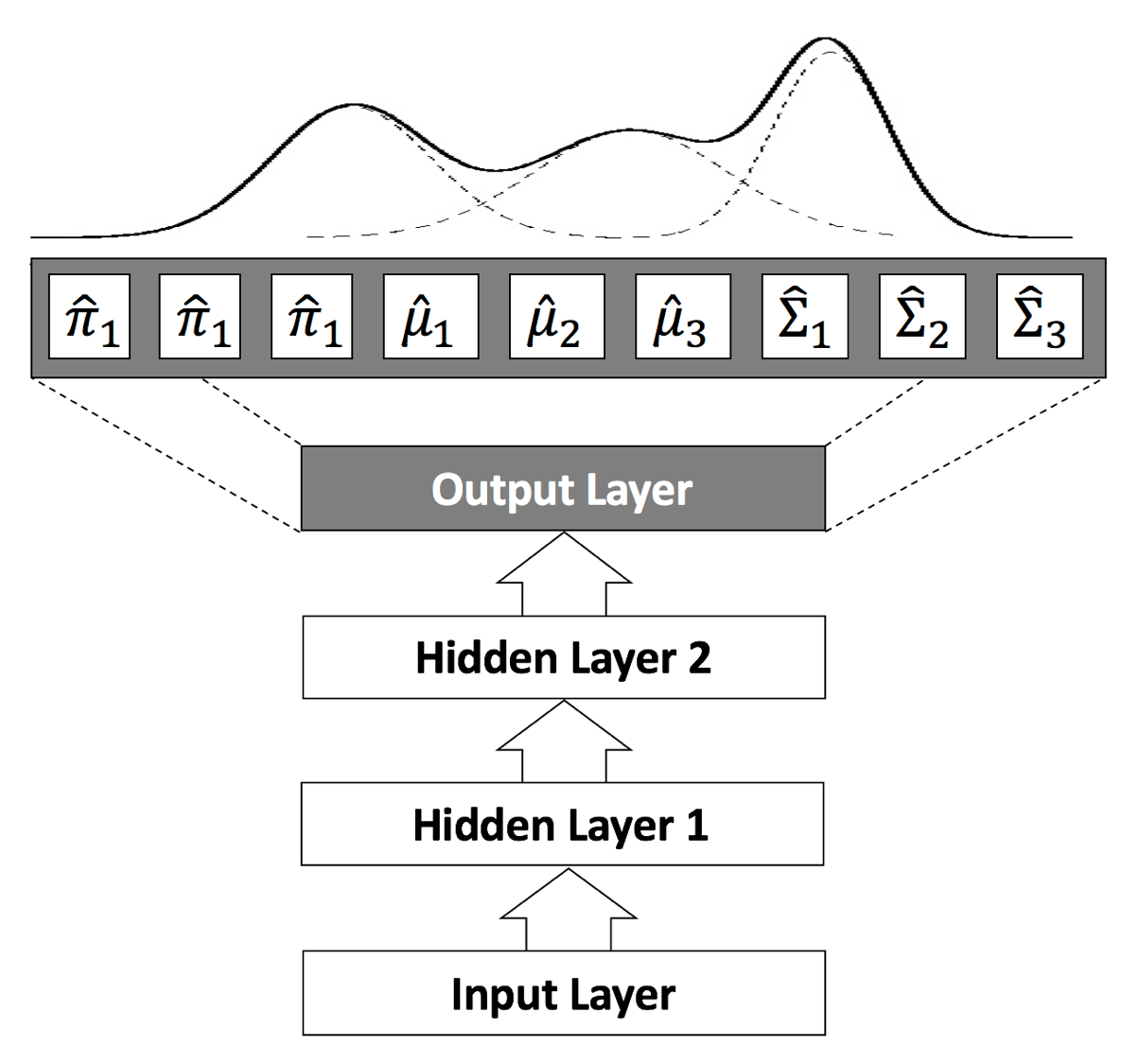
Figure 1: A mixture density network ($K=3$) with two hidden layers where the output of the network is decomposed into $\hat{\pi}$, $\hat{\mu}$, and $\hat{\Sigma}$.

A mixture density network (MDN) was first proposed in [7] where the output of a neural network is composed of parameters constructing a Gaussian mixture model (GMM):

$$p(\mathbf{y}|\theta)=\sum_{j=1}^{K}\pi_{j}\mathcal{N}(\mathbf{y}|\mu_{j},\,\Sigma_{j})$$

where $\theta=\{\pi_{j},\mu_{j},\Sigma_{j}\}_{j=1}^{K}$ is a set of parameters of a GMM, mixture probabilities, mixture means, and mixture variances, respectively. In other words, an MDN can be seen as a mapping $f$ from an input $\mathbf{x}\in\mathbf{X}$ to the parameters $\theta\in\Theta$ of a GMM of an output, i.e., $f:\mathbf{X}\mapsto\Theta$ as shown in Figure 1.

However, as mixture weights should be on a $K$ dimensional simplex and each mixture variance should be positive definite, the output of an MDN is handled accordingly. We assume that each output dimension is independent, and each mixture variance becomes a diagonal matrix. Suppose that the dimension of the output $\mathbf{y}$ is $d$ and let $\{\hat{\pi}_{j},\hat{\mu}_{j},\hat{\Sigma}_{j}\}_{j=1}^{K}$ be the raw output of an MDN where $\hat{\pi}_{j}\in{\mathbb{R}}$, $\hat{\mu}_{j}\in{\mathbb{R}}^{d}$, and $\hat{\Sigma}_{j}\in{\mathbb{R}}^{d}$. Then the parameters of a GMM is computed by

$$\pi_{j} =\frac{\exp\left(\hat{\pi}_{j}-\max(\pi)\right)}{\sum_{k=1}^{K}\exp(\hat{\pi}_{k}-\max(\pi))}$$ (2)

$$\mu_{j} =\hat{\mu_{j}}$$

$$\Sigma_{j} =\sigma_{max}{\textrm{diag}}\left(\rho(\hat{\Sigma}_{j})\right)$$ (3)

where $\max(\pi)$ indicates the maximum mixture weights among all $K$ weights, ${\textrm{diag}}(\cdot)$ is an operation to convert a $d$-dimensional vector to a $d\times d$-dimensional diagonal matrix, and $\rho(x)=\frac{1}{1+\exp(-x)}$ is an element-wise sigmoid function.

Two heuristics are applied in (2) and (3). First, we found that exponential operations often cause numerical instabilities, and thus, subtracted the maximum mixture value in (2). In (3), similarly, we used a sigmoid function multiplied by a constant instead of an exponential function to satisfy the positiveness constraint of the variance. $\sigma_{max}$ is selected manually and set to five throughout the experiments.

For training the MDN, we used a negative log likelihood as a cost function

$$c(\theta;\mathcal{D})=-\frac{1}{N}\sum_{i=1}^{N}\log(\sum_{j=1}^{K}\pi_{j}(\mathbf{x}_{i})\mathcal{N}(\mathbf{y}_{i}|\mu_{j}(\mathbf{x}_{i}),\,\Sigma_{j}(\mathbf{x}_{i}))+\epsilon)$$ (4)

where $\mathcal{D}=\{(\mathbf{x}_{i},\mathbf{y}_{i})\}_{i=1}^{N}$ is a set of training data and $\epsilon=10^{-6}$ is for numerical stability of a logarithm function. We would like to note that an MDN can be implemented on top of any deep neural network architectures, e.g., a multi-layer perceptron, convolutional neural network, or recurrent neural network.

Once an MDN is trained, the predictive mean and variance can be computed by selecting the mean and variance of the mixture of the highest mixture weight (MAP estimation). This can be seen as a mixture of experts [18] where the mixture weights form a gating network for selecting local experts.

IV Proposed Uncertainty Estimation Method

In this section, we propose a novel uncertainty acquisition method for a regression task using a mixture density network (MDN) using a law of total variance [19]. As described in Section III-B, an MDN constitutes a Gaussian mixture model (GMM) of an output $\mathbf{y}$ given a test input $\mathbf{x}$:

$$p(\mathbf{y}|\mathbf{x})=\sum_{j=1}^{K}\pi_{j}(\mathbf{x})\mathcal{N}\left(\mathbf{y};\mu_{j}(\mathbf{x}),\,\Sigma_{j}(\mathbf{x})\right)$$ (5)

where $\pi_{j}(\mathbf{x})$, $\mu_{j}(\mathbf{x})$, and $\Sigma_{j}(\mathbf{x})$ are $j$-th mixture weight function, mean function, and variance function, respectively. Note that a GMM can approximate any given density function to arbitrary accuracy [12]. While the number of mixtures becomes prohibitively large to achieve this, it is worthwhile noting that an MDN is more suitable for fitting complex and noisy distribution compared to a density network.

IV-A Uncertainty Acquisition for a Mixture Density Network

Let us first define the total expectation of a GMM.

$$\mathbb{E}[\mathbf{y}|\mathbf{x}] =\sum_{j=1}^{K}\pi_{j}(\mathbf{x})\int\mathbf{y}\mathcal{N}(\mathbf{y};\mu_{j}(\mathbf{x}),\Sigma_{j}(\mathbf{x}))d\mathbf{y}$$

$$=\sum_{j=1}^{K}\pi_{j}(\mathbf{x})\mu_{j}(\mathbf{x})$$ (6)

The total variance of a GMM is computed as follows (we omit $\mathbf{x}$ in each function).

$$\mathbb{V}(\mathbf{y}|\mathbf{x}) =\int\left\|\mathbf{y}-\mathbb{E}\left[\mathbf{y}|\mathbf{x}\right]\right\|^{2}p(\mathbf{y}|\mathbf{x})d\mathbf{y}$$

$$=\sum_{j=1}^{K}\pi_{j}\int\left\|\mathbf{y}-\sum_{k=1}^{K}\pi_{k}\mu_{k}\right\|^{2}\mathcal{N}(\mathbf{y};\mu_{j},\Sigma_{j})d\mathbf{y}$$

where the term inside the integral becomes

$$\int \left\|\mathbf{y}-\sum_{k=1}^{K}\pi_{k}\mu_{k}\right\|^{2}\mathcal{N}(\mathbf{y};\mu_{j},\Sigma_{j})d\mathbf{y}$$

$$=\int\left\|\mathbf{y}-\mu_{j}\right\|^{2}\mathcal{N}(\mathbf{y};\mu_{j},\Sigma_{j})d\mathbf{y}$$

$$\qquad+\int\left\|\mu_{j}-\sum_{k=1}^{K}\pi_{k}\mu_{k}\right\|^{2}\mathcal{N}(\mathbf{y};\mu_{j},\Sigma_{j})d\mathbf{y}$$

$$\qquad\quad+2\int(\mathbf{y}-\mu_{j})^{T}(\mu_{j}-\sum_{k=1}^{K}\pi_{k}\mu_{k})\mathcal{N}(\mathbf{y};\mu_{j},\Sigma_{j})d\mathbf{y}$$

$$=\Sigma_{j}+\left\|\mu_{j}-\sum_{k=1}^{K}\pi_{k}\mu_{k}\right\|^{2}.$$

Therefore the total variance $\mathbb{V}(\mathbf{y}|\mathbf{x})$ becomes (also see (47) in [7]):

$$\mathbb{V}(\mathbf{y}|\mathbf{x}) =\sum_{j=1}^{K}\pi_{j}(\mathbf{x})\Sigma_{j}(\mathbf{x})$$

$$\quad+\sum_{j=1}^{K}\pi_{j}(\mathbf{x})\left\|\mu_{j}(\mathbf{x})-\sum_{k=1}^{K}\pi_{k}(\mathbf{x})\mu_{k}(\mathbf{x})\right\|^{2}.$$ (7)

Now let us present the connection between the two terms in (7) that constitute the total variance of a GMM to the epsitemic uncertainty and aleatoric uncertainty in [6].

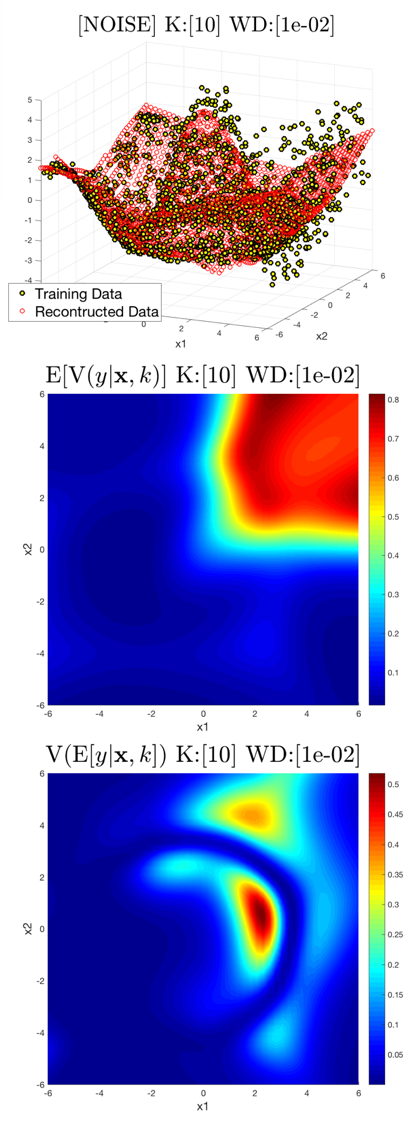
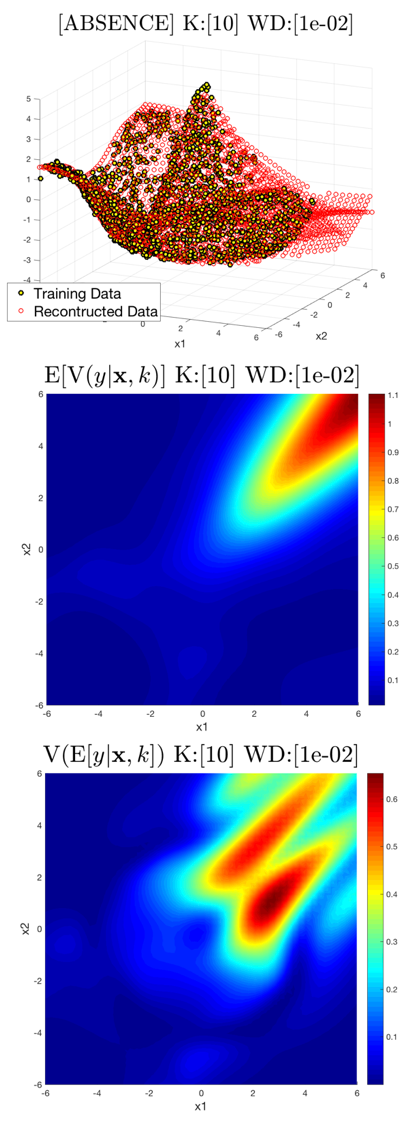
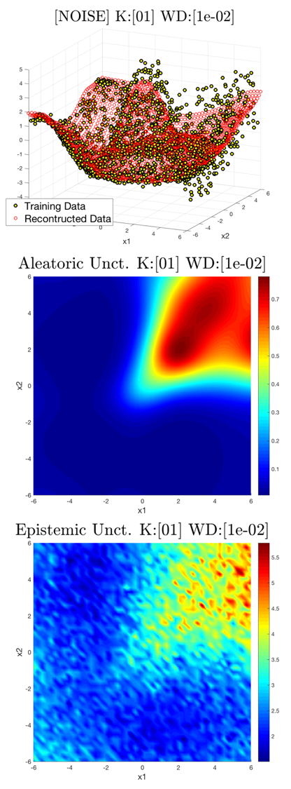
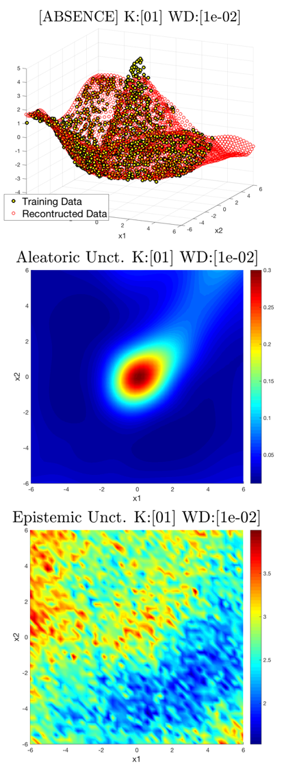
Figure 2: Proposed uncertainty measures of a) heavy noise and b) absence of data scenarios and Aleatoric and epistemic uncertainties of (c) heavy noise and (d) absence of data scenarios.

IV-B Connection to Aleatoric and Epistemic Uncertainties

Let $\sigma_{\mathfrak{a}}$ and $\sigma_{\mathfrak{e}}$ be aleatoric uncertainty and epistemic uncertainty, respectively. Then, these two uncertainties constitute total predictive variance as shown in Section III-A.

$$\mathbb{V}(\mathbf{y}|\mathbf{x})=\sigma_{\mathfrak{a}}^{2}(\mathbf{x})+\sigma_{\mathfrak{e}}^{2}(\mathbf{x})$$

On the other hand, we can rewrite (7) as

$$\mathbb{V}\left(\mathbf{y}|\mathbf{x}\right) =\mathbb{V}_{k\sim\pi}\left(\mathbb{E}\left[\mathbf{y}|\mathbf{x},k\right]\right)+\mathbb{E}_{k\sim\pi}\left(\mathbb{V}\left(\mathbf{y}|\mathbf{x},k\right)\right).$$

We remark that $\mathbb{V}_{k\sim\pi}(\mathbb{E}[\mathbf{y}|\mathbf{x},k])$ indicates explained variance whereas $\mathbb{E}_{k\sim\pi}\left[\mathbb{V}(\mathbf{y}|\mathbf{x},k)\right]$ represents unexplained variance [19]. Observe that

$$\mathbb{V}_{k\sim\pi}(\mathbb{E}[\mathbf{y}|\mathbf{x},k])=\mathbb{V}_{k\sim\pi}\left(\mu_{k}(\mathbf{x})\right)$$

$$=\sum_{k=1}^{K}\pi_{k}(\mathbf{x})\left\|\mu_{k}(\mathbf{x})-\sum_{j=1}^{K}\pi_{j}(\mathbf{x})\mu_{j}(\mathbf{x})\right\|^{2}$$ (8)

$$\mathbb{E}_{k\sim\pi}[\mathbb{V}(\mathbf{y}|\mathbf{x},k)]=\mathbb{E}_{k\sim\pi}\left[\Sigma_{k}(\mathbf{x})\right]=\sum_{k=1}^{K}\pi_{k}(\mathbf{x})\Sigma_{k}(\mathbf{x})$$ (9)

This implies that (7) can be decomposed into uncertainty quantity of each mixture, i.e.,

$$\sigma_{\mathfrak{a}}^{2}(\mathbf{x}|k) +\sigma_{\mathfrak{e}}^{2}(\mathbf{x}|k)$$

$$=\Sigma_{k}(\mathbf{x})+\left\|\mu_{k}(\mathbf{x})-\sum_{j=1}^{K}\pi_{j}(\mathbf{x})\mu_{j}(\mathbf{x})\right\|^{2}.$$ (10)

$\Sigma_{k}(\mathbf{x})$ in the right hand side of (10) is the predicted variance of the $k$-th mixture where it can be interpreted as aleatoric uncertainty as the variance of a density network captures the noise inherent in data [16]. Consequently, $\left\|\mu_{k}(\mathbf{x})-\sum_{j=1}^{K}\pi_{j}(\mathbf{x})\mu_{j}(\mathbf{x})\right\|^{2}$ corresponds to the epistemic uncertainty estimating our ignorance about the model prediction. We validate these connections with both synthetic examples and track driving demonstrations in Section V and VI.

We would like to emphasize that Monte Carlo (MC) sampling is not required to compute the total variance of a GMM as we introduced randomness from the mixture distribution $\pi$. The predictive variance (1) proposed in in [6] requires MC sampling with random weight masking. This additional sampling is required as the density network can only model a single mean and variance. However, when using the MDN, it can not only model the measurement noise or aleatoric uncertainty $\sigma^{2}_{a}$ with (9) but also model our ignorance about the model through (8). Intuitively speaking, (8) becomes high when the mean function of each mixture does not match the total expectation and will be used to model in uncertainty-aware learning from demonstration in Section VI.

V Analysis of the Proposed Uncertainty Modeling with Synthetic Examples

In this section, we analyze the properties of the proposed uncertainty modeling method in Section IV with three carefully designed synthetic examples: absence of data, heavy noise, and composition of functions scenarios. In all experiments, fully connected networks with two hidden layers, $256$ hidden nodes, and tanh activation function is used and the number of mixtures is $10$. We also implemented the algorithm in [6] with the same network topology and used $50$ Monte Carlo (MC) sampling for computing the predictive variance as shown in the original paper. The keep probability of dropout is $0.8$ and all codes are implemented with TensorFlow [20]

In the absence of data scenario, we removed the training data on the first quadrant and show how different each type of uncertainty measure behaves on the input regions with and without training data. For the heavy noise scenario, we added heavy uniform noises from $-2$ to $+2$ to the outputs training data whose inputs are on the first quadrant. The input space and underlying function for both absence of data and heavy noise are $f(\mathbf{x})=5\cos(\frac{\pi}{2}\|\frac{\mathbf{x}}{2}\|)\exp(-\frac{\pi\|\mathbf{x}\|}{20})$ and $\mathbb{X}=\{\mathbf{x}=(x_{1},x_{2})|-6\leq x_{1},x_{2}\leq+6\}$, respectively. These two scenarios are designed to validate whether the proposed method can distinguish unfamiliar inputs from inputs with high measurement errors. We believe this ability of knowing its ignorance is especially important when it comes to deploy a learning-based system to an actual physical system involving humans.

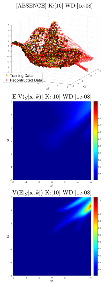
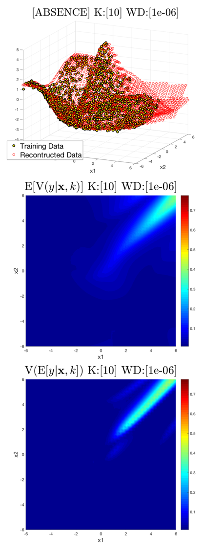
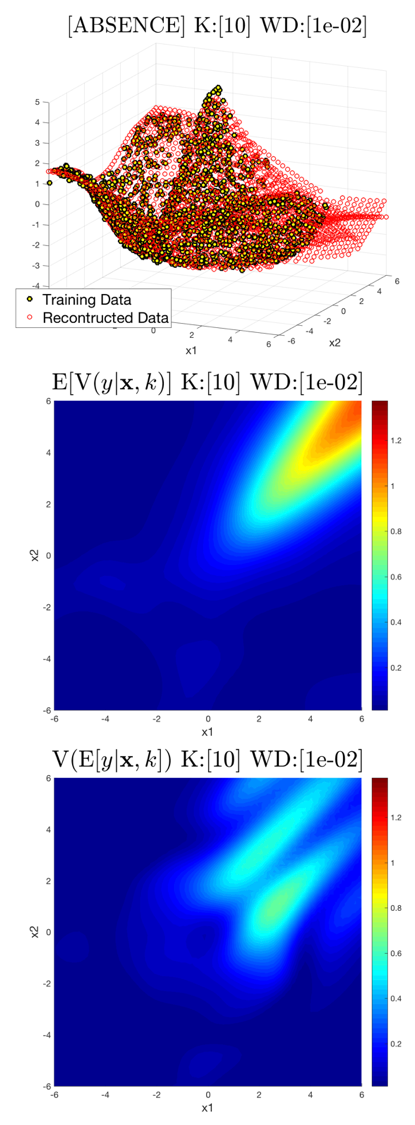
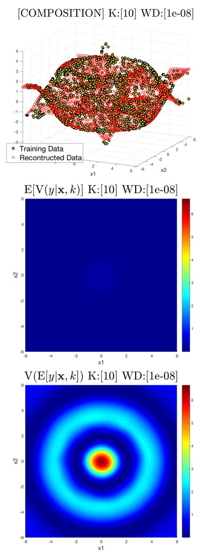
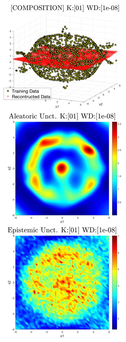
Figure 3: Proposed uncertainty measures of the heavy noise scenario while varying the weight decay levels (a-c) and the composition of functions scenario (d). (e) Aleatoric and epistemic uncertainties of composition of functions scenario.

In the composition of functions scenario, the training data are collected from two different function $f(\mathbf{x})$ and flipped $-f(\mathbf{x})$. This scenario is designed to reflect the cases where we have multiple but few choices to select. For example, when there is a car in front, there could be roughly two choices to select, turn left or turn right, where both choices are totally fine. If the learned model can distinguish this from noisy measurements, it could give additional information to the overall system.

As explained in Section IV, the proposed uncertainty measure is composed of two terms $\mathrm{V}(\mathrm{E}[y|\mathbf{x},k])$ and $\mathrm{E}[\mathrm{V}(y|\mathbf{x},k)]$ where the sum is the total predictive variance $\mathrm{V}(y|\mathbf{x})$. Before starting the analysis, let us state again the connections between $\mathrm{V}(\mathrm{E}[y|\mathbf{x},k])$ and $\mathrm{E}[\mathrm{V}(y|\mathbf{x},k)]$ of the proposed method and aleatoric and epistemic uncertainties proposed in [6]. $\mathrm{V}(\mathrm{E}[y|\mathbf{x},k])$ indicates explained variance which corresponds to epistemic uncertainty and it indicate our ignorance about the model. On the other hand, $\mathrm{E}[\mathrm{V}(y|\mathbf{x},k)]$ models unexplained variance and it corresponds to aleatoric uncertainty indicating measurement noises or randomness inherent in the data generating process.

In Figure 2 and 2, the proposed uncertainty measures, $\mathrm{V}(\mathrm{E}[y|\mathbf{x},k])$, $\mathrm{E}[\mathrm{V}(y|\mathbf{x},k)]$, and $\mathrm{V}(y|\mathbf{x})$ of both heavy noise and absence of data scenarios are illustrated. The uncertainty measures in [6], epistemic uncertainty and aleatoric uncertainty, are shown in Figure 2 and 2.

First, in the heavy noise scenario, both proposed method and the method in [6] capture noisy regions as illustrated in Figure 2 and 2. Particularly, $\mathrm{E}[\mathrm{V}(y|\mathbf{x},k)]$ in Figure 2 and epistemic uncertainty in Figure 2 correctly depicts the region with heavy noise. This is mainly because measurement noise is related to the aleatoric uncertainty which could easily be captured with density networks.

	$\mathrm{E}[\mathrm{V}(y|\mathbf{x},k)]$	$\mathrm{V}(\mathrm{E}[y|\mathbf{x},k])$
Heavy noise	High	High or Low
Absence of data	High	High
Composition of functions	Low	High

TABLE I: Summary of $\mathrm{E}[\mathrm{V}(y|\mathbf{x},k)]$ and $\mathrm{V}(\mathrm{E}[y|\mathbf{x},k])$ on absence of data, heavy noise, and composition of functions scenarios.

	Computation Time [ms]
Proposed method	$48.08$
[6]	$1209.12$

TABLE II: Summary of Computation time for estimating the proposed $\mathrm{E}[\mathrm{V}(y|\mathbf{x},k)]$ and $\mathrm{V}(\mathrm{E}[y|\mathbf{x},k])$ vs. aleatoric and epistemic uncertainties in [6] where we run the MC sampling for $50$ times.

However, when it comes to the absence of data scenario, proposed and compared methods show clear difference. While both aleatoric and epistemic uncertainties in Figure 2 can hardly capture the regions with no training data, the proposed method shown in Figure 2 effectively captures such regions by assigning high uncertainties to unseen regions. In particular, it can be seen that $\mathrm{V}(\mathrm{E}[y|\mathbf{x},k])$ captures this region more suitably compared to $\mathrm{E}[\mathrm{V}(y|\mathbf{x},k)]$. This is a reasonable result in that $\mathrm{V}(\mathrm{E}[y|\mathbf{x},k])$ is related to the epistemic uncertainty which represents the model uncertainty, i.e., our ignorance about the model.

This difference between $\mathrm{V}(\mathrm{E}[y|\mathbf{x},k])$ and $\mathrm{E}[\mathrm{V}(y|\mathbf{x},k)]$ becomes more clear when we compare $\mathrm{V}(\mathrm{E}[y|\mathbf{x},k])$ of absence of data and heavy noise scenarios. Unlike absence of data scenario where $\mathrm{V}(\mathrm{E}[y|\mathbf{x},k])$ is high in the first quadrant (data-absence region), $\mathrm{V}(\mathrm{E}[y|\mathbf{x},k])$ in this region contains both high and low variances. This is mainly due to the fact that $\mathrm{V}(\mathrm{E}[y|\mathbf{x},k])$ is related to the epistemic uncertainty which can be explained away with more training data (even with high measurement noise).

It is also interesting to see the effect of the prior information of weight matrices. In Bayesian deep learning, a prior distribution is given to the weight matrices to assign posterior probability distribution over the outputs [11]. In this perspective, $L_{2}$ weight decay on the weight matrices can be seen as assigning a Gaussian prior over the weight matrices. Figure 3, 3, and 3 show $\mathrm{V}(\mathrm{E}[y|\mathbf{x},k])$, $\mathrm{E}[\mathrm{V}(y|\mathbf{x},k)]$, and $\mathrm{V}(y|\mathbf{x})$ of the absence of data scenario with different weight decay levels. One can clearly see that the regions with no training data are more accurately captured as we increase the weight decay level. Specifically, $\mathrm{E}[\mathrm{V}(y|\mathbf{x},k)]$ is more affected by the weight decay level as it corresponds to aleatoric uncertainty which is related to the weight decay level [11]. Readers are referred to Section 6.7 in [11] for more information about the effects of weight decay and dropout to a Bayesian neural network.

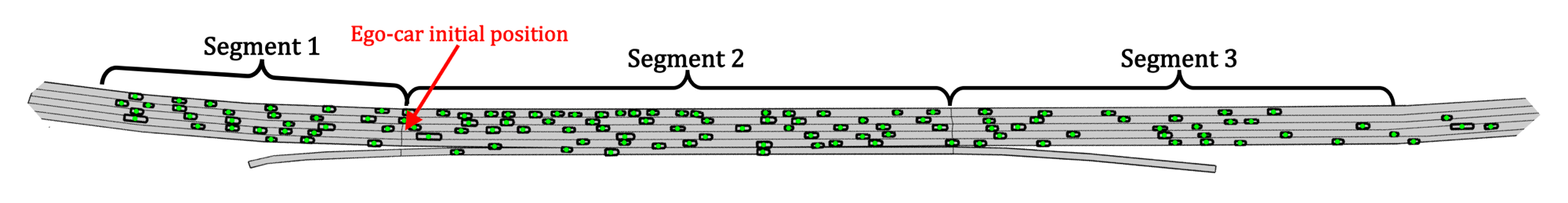
Figure 4: A snapshot of NGSIM track environmet.

Figure 3 and 3 shows the experimental results in the composition of functions scenario. As a single density network cannot model the composite of two functions, the reconstructed results shown with red circles in Figure 3 are poor as well as aleatoric and epistemic uncertainties. On the other hand, the reconstructed results from the MDN with $10$ mixtures accurately model the composition of two function. Furthermore, $\mathrm{E}[\mathrm{V}(y|\mathbf{x},k)]$ and $\mathrm{V}(\mathrm{E}[y|\mathbf{x},k])$ show clear differences. In particular, $\mathrm{E}[\mathrm{V}(y|\mathbf{x},k)]$ is low on almost everywhere whereas $\mathrm{V}(\mathrm{E}[y|\mathbf{x},k])$ has both high and low variances which is proportional to the difference between two composite function. As the training data itself does not contain any measurement noises, $\mathrm{E}[\mathrm{V}(y|\mathbf{x},k)]$ has low values in its input domain. However, $\mathrm{V}(\mathrm{E}[y|\mathbf{x},k])$ becomes high where the differences between two possible outputs are high, as it becomes more hard to fit the training data in such regions.

Table II summarizes how $\mathrm{E}[\mathrm{V}(y|\mathbf{x},k)]$ and $\mathrm{V}(\mathrm{E}[y|\mathbf{x},k])$ behave on three different scenarios. The computation times for the proposed method and compared method [6] is shown in Table II where the proposed method is about $21.15$ times faster as it does not require MC sampling.

VI Uncertainty-Aware Learning from Demonstration to Drive

We propose uncertainty-aware LfD (UALfD) which combines the learning-based approach with a rule-based approach by switching the mode of the controller using the uncertainty measure in Section V. In particular, explained variance (8) is used as a measure of uncertainty as it estimates the model uncertainty. The proposed method makes the best of both approaches by using the model uncertainty as a switching criterion. The proposed UALfD is applied to an aggressive driving task using a real-world driving dataset [13] where the proposed method significantly improves the performance of driving in terms of both safety and efficiency by incorporating the uncertainty information.

For evaluating the proposed uncertainty-aware learning from demonstration method, we use the Next-Generation Simulation (NGSIM) datasets collected from US Highway 101 [13] which provides $45$ minutes of real-world vehicle trajectories at $10$Hz as well as CAD files for road descriptions. Figure 4 illustrates the road configuration of US Highway 101, which consists of three segments and six lanes. For testing, we only used the second segment, where the initial position of an ego car is at the start location of the third lane in the second segment and the goal is to reach the third segment. Once the ego-car is outside the track or collide with other cars, it is counted as a collision.

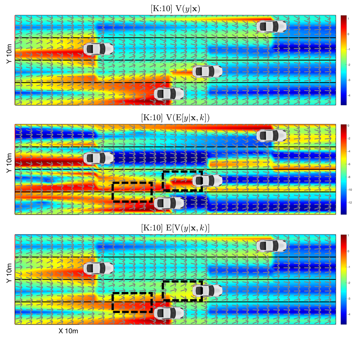
Figure 5: Different uncertainty measures on tracks.

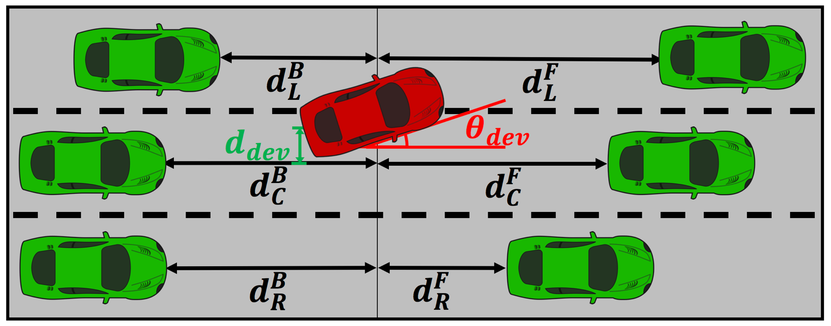
Figure 6: Feature descriptions for the track driving scenarios.

To efficiently collect a sufficient number of driving demonstrations, we use density matching reward learning [21] to automatically generate driving demonstrations in diverse environments by randomly changing the initial position of an ego car and configurations of other cars. Demonstrations with collisions are excluded from the dataset to form collision-free trajectories. However, it is also possible to manually collect an efficient number of demonstrations using human-in-the loop simulations.

We define a learning-based driving policy $\pi$ as a mapping from input features to the trigonometric encoded desired heading angle of a car, $(\cos\theta_{dev},\,\sin\theta_{dev})$. Figure 6 illustrates obtainable features of the track driving simulator. A seven-dimensional frontal and rearward feature representation, which consists of three frontal distances to the closest cars in left, center, and right lanes in the front, three rearward distances to the closest cars in left, center, and right lanes in the back, and lane deviate distance, $(d^{F}_{L},\,d^{F}_{C},\,d^{F}_{R},d^{B}_{L},\,d^{B}_{C},\,d^{B}_{R},\,d_{dev})$, are used as the input representation.

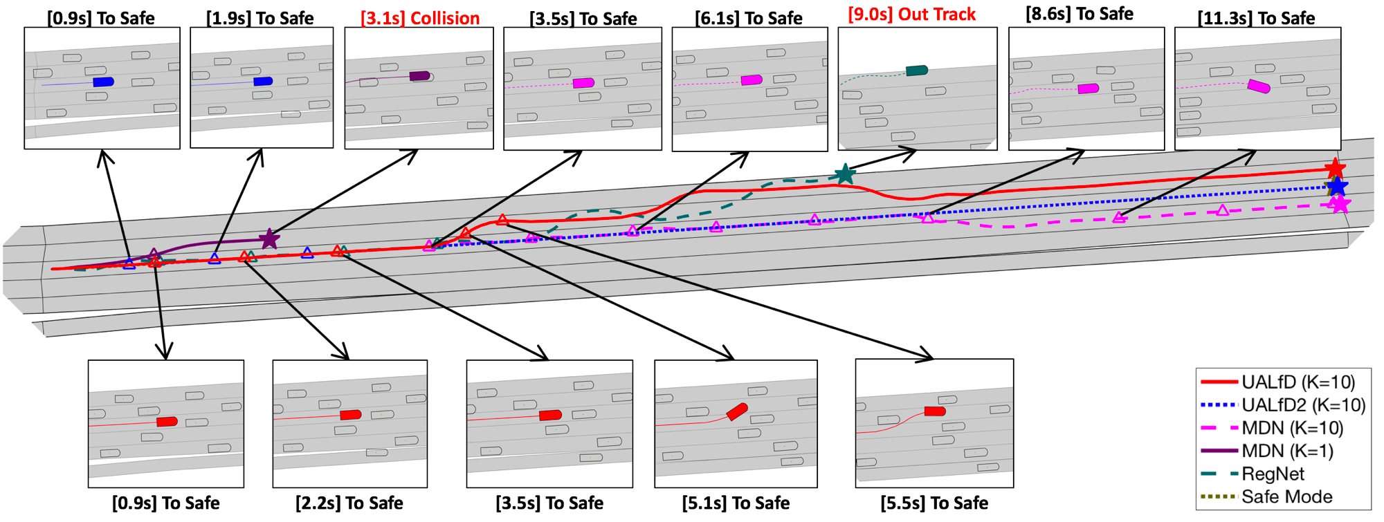
Figure 7: Snapshots of driving results of different LfD methods.

	Collision Ratio [%]	Min. Dist. to Cars	Lane Dev. Dist. [mm]	Lane Dev. Deg.	Elapsed Time [s]	Num. Lane Change
UALfD (K=10)	$\mathbf{0.00}$	$3.67$	$154.29$	$2.13$	$15.83$	$1.62$
UALfD2 (K=10)	$\mathbf{0.00}$	$6.48$	$75.56$	$0.94$	$17.47$	$0.09$
MDN (K=10)	$7.55$	$3.43$	$289.01$	$3.41$	$16.40$	$1.67$
MDN (K=1)	$15.09$	$3.34$	$373.03$	$3.94$	$17.22$	$1.38$
RegNet	$28.30$	$3.49$	$393.48$	$4.86$	$17.42$	$2.05$
Safe Mode	$0.00$	$13.59$	$5.78$	$0.06$	$18.46$	$0.00$

TABLE III: Quantitative driving results in NGSIM dataset.

	Collision Ratio [%]	Min. Dist. to Cars	Lane Dev. Dist. [mm]	Lane Dev. Deg.	Elapsed Time [s]	Num. Lane Change
UALfD (K=10)	$\mathbf{0.00}$	$4.28$	$197.03$	$2.80$	$15.54$	$2.52$
UALfD2 (K=10)	$1.16$	$6.68$	$113.38$	$1.43$	$18.26$	$0.04$
MDN (K=10)	$3.49$	$4.15$	$286.07$	$3.54$	$15.60$	$2.05$
MDN (K=1)	$25.58$	$4.05$	$368.23$	$3.91$	$16.19$	$2.42$
RegNet	$41.86$	$4.49$	$403.08$	$5.01$	$17.79$	$2.52$
Safe Mode	$1.16$	$23.57$	$5.54$	$0.06$	$20.71$	$0.00$

TABLE IV: Quantitative driving results in NGSIM dataset with $80\%$ of cars.

We trained three different network configurations: an MDN with ten mixtures, MDN (K=10), MDN with one mixture, MDN (k=1), and a baseline fully connected layer, RegNet, trained with a squared loss. All networks have two hidden layers with $256$ nodes where a $tanh$ activation function is used. The proposed uncertainty-aware learning from demonstration method, UALfD, switches its mode to the safe policy when the $\log$ of explained variance is higher that $-2$. As the variance is not scaled, we manually tune the threshold. However, we can chose the threshold based on the percentile of an empirical cumulative probability distribution similar to [17]. We also implemented uncertainty-aware learning from demonstration method, UALfD2 which utilizes $\mathrm{E}[\mathrm{V}(y|\mathbf{x},k)]$ instead of $\mathrm{V}(\mathrm{E}[y|\mathbf{x},k])$ to justify the usage of using $\mathrm{V}(\mathrm{E}[y|\mathbf{x},k])$ as an uncertainty measure of LfD. To avoid an immediate collision, UALfD switches to the safe mode when $d^{F}_{C}$ is below $1.5\,m$ and other methods switches when $d^{F}_{C}$ is below $2.5\,m$.

Figure 5 illustrates total variance $\mathrm{V}(y|\mathbf{x})$, explainable variance $\mathrm{V}(\mathrm{E}[y|\mathbf{x},k])$, and unexplained varaince $\mathrm{E}[\mathrm{V}(y|\mathbf{x},k)]$ estimated using an MDN with ten mixtures at each location. Here, we can see clear differences between $\mathrm{V}(\mathrm{E}[y|\mathbf{x},k])$ and $\mathrm{E}[\mathrm{V}(y|\mathbf{x},k)]$ in two squares with black dotted lines where $\mathrm{V}(\mathrm{E}[y|\mathbf{x},k])$ can better capture model uncertainty possibly due to the lack of training data. Furthermore, we can see that the regions where the desirable heading depicted with gray arrows are not accurate, e.g., leading to a collision, has higher variance and it does not necessarily depend on the distance between the frontal car. This supports that our claim in that $\mathrm{V}(\mathrm{E}[y|\mathbf{x},k])$ is more suitable for estimating modeling error.

Once a desired heading is achieved, the ego-car is controlled at $10$Hz using a simple feedback controller for an angular velocity $w$ with $w=\min(2\cdot\text{sign}(\theta_{diff})\cdot\theta_{diff}^{2},w_{max})$ where $\theta_{diff}$ is the difference between current heading and desired heading from the learned controller normalized between $-180$ to $+180degree$. A directional velocity is fixed at $90\,$km/h and the control frequency is set to $10\,$Hz. While we use a simple unicycle dynamic model, more complex dynamic models, e.g., vehicle and bicycle dynamic models, can be also used.

We also carefully designed a rule-based safe controller that safely keeps its lane without a collision where the directional and angular velocities are computed by following rules:

$$v =\begin{cases}v^{F}_{C}-5\,\text{m/s},&\text{if $d^{F}_{C}<3$}\\ v^{R}_{C}+3\,\text{m/s},&\text{if $d^{R}_{C}<3$}\\ \frac{v^{F}_{C}+v^{R}_{C}}{2},&\text{otherwise}\end{cases}$$

$$w =-5*\theta_{dev}+50*d_{dev}$$

where $v^{F}_{C}$ and $v^{R}_{C}$ are the directional velocities of the frontal and rearward cars, respectively.

We conducted two sets of experiments, one with using the entire cars and the other with using $70\%$ of the cars. The quantitative results are shown in Table IV and IV. The results show that the driving policy that incorporates the proposed uncertainty measure clearly improves both safety and stability of driving. We would like to emphasize that the average elapsed time of the propose UALfD is the shortest among the compared method. Figure 7 shows trajectories and some snapshots of driving results of different methods. Among compared methods, the proposed UALfD, UALfD2, MDN (K=10), and Safe Mode safely navigates without colliding with other moving cars. On the other hand, the cars controlled with MDN (K=1) and RegNet collide with another car and move outside the track which clearly shows the advantage of using a mixture density network for modeling human demonstrations. Furthermore, while both UALfD and UALfD2 navigate without a collision, the average elapsed time and the average number lane changes varies greatly. This is mainly due to the fact that $\mathrm{E}[\mathrm{V}(y|\mathbf{x},k)]$ captures the measure noise rather than the model uncertainty which makes the control conservative similar to that of the Safe Mode.

VII Conclusion

In this paper, we proposed a novel uncertainty estimation method using a mixture density network. Unlike existing approaches that rely on ensemble of multiple models or Monte Carlo sampling with stochastic forward paths, the proposed uncertainty acquisition method can run with a single feedforward model without computationally-heavy sampling. We show that the proposed uncertainty measure can be decomposed into explained and unexplained variances and analyze the properties with three different cases: absence of data, heavy measurement noise, and composition of functions scenarios and show that it can effectively distinguish the three cases using the two types of variances. Furthermore, we propose an uncertainty-aware learning from demonstration method using the proposed uncertainty estimation and successfully applied to real-world driving dataset.

References

- [1] K. He, X. Zhang, S. Ren, and J. Sun, “Deep residual learning for image recognition,” in Proc. of the IEEE conference on Computer Vision and Pattern Recognition, 2016, pp. 770–778.
- [2] R. Collobert and J. Weston, “A unified architecture for natural language processing: Deep neural networks with multitask learning,” in Proc. of the International Conference on Machine Learning, 2008, pp. 160–167.
- [3] J. Schulman, S. Levine, P. Abbeel, M. I. Jordan, and P. Moritz, “Trust region policy optimization.” in Proc. of the International Conference on Machine Learing, 2015, pp. 1889–1897.
- [4] D. Amodei, C. Olah, J. Steinhardt, P. Christiano, J. Schulman, and D. Mané, “Concrete problems in ai safety,” arXiv preprint arXiv:1606.06565, 2016.
- [5] AP and REUTERS, “Tesla working on ’improvements’ to its autopilot radar changes after model s owner became the first self-driving fatality.” June 2016. [Online]. Available: https://goo.gl/XkzzQd
- [6] A. Kendall and Y. Gal, “What uncertainties do we need in Bayesian deep learning for computer vision?” arXiv preprint arXiv:1703.04977, 2017.
- [7] C. M. Bishop, “Mixture density networks,” 1994.
- [8] A. Brando Guillaumes, “Mixture density networks for distribution and uncertainty estimation,” Master’s thesis, Universitat Politècnica de Catalunya, 2017.
- [9] B. Lakshminarayanan, A. Pritzel, and C. Blundell, “Simple and scalable predictive uncertainty estimation using deep ensembles,” arXiv preprint arXiv:1612.01474, 2016.
- [10] Y. Gal and Z. Ghahramani, “Dropout as a Bayesian approximation: Representing model uncertainty in deep learning,” in Proc. of the International Conference on Machine Learing, 2016, pp. 1050–1059.
- [11] Y. Gal, “Uncertainty in deep learning,” Ph.D. dissertation, PhD thesis, University of Cambridge, 2016.
- [12] G. J. McLachlan and K. E. Basford, Mixture models: Inference and applications to clustering. Marcel Dekker, 1988, vol. 84.
- [13] J. Colyar and J. Halkias, “Us highway 101 dataset,” Federal Highway Administration (FHWA), Tech. Rep., 2007.
- [14] S. Ross, “Interactive learning for sequential decisions and predictions,” Ph.D. dissertation, Carnegie Mellon University, 2013.
- [15] N. Srivastava, G. E. Hinton, A. Krizhevsky, I. Sutskever, and R. Salakhutdinov, “Dropout: a simple way to prevent neural networks from overfitting.” Journal of machine learning research, vol. 15, no. 1, pp. 1929–1958, 2014.
- [16] G. Kahn, A. Villaflor, V. Pong, P. Abbeel, and S. Levine, “Uncertainty-aware reinforcement learning for collision avoidance,” arXiv preprint arXiv:1702.01182, 2017.
- [17] C. Richter and N. Roy, “Safe visual navigation via deep learning and novelty detection,” in Proc. of the Robotics: Science and Systems Conference, 2017.
- [18] N. Shazeer, A. Mirhoseini, K. Maziarz, A. Davis, Q. Le, G. Hinton, and J. Dean, “Outrageously large neural networks: The sparsely-gated mixture-of-experts layer,” arXiv preprint arXiv:1701.06538, 2017.
- [19] R. O. Duda, P. E. Hart, and D. G. Stork, Pattern classification. Wiley, New York, 1973.
- [20] M. Abadi, A. Agarwal, P. Barham, E. Brevdo, Z. Chen, C. Citro, G. S. Corrado, A. Davis, J. Dean, M. Devin et al., “Tensorflow: Large-scale machine learning on heterogeneous distributed systems,” arXiv preprint arXiv:1603.04467, 2016.
- [21] S. Choi, K. Lee, A. Park, and S. Oh, “Density matching reward learning,” arXiv preprint arXiv:1608.03694, 2016.