Normalized Features for Improving the Generalization of DNN Based Speech Enhancement

Abstract

Enhancing noisy speech is an important task to restore its quality and to improve its intelligibility. In traditional non-ML based approaches the parameters required for noise reduction are estimated blindly from the noisy observation while the actual filter functions are derived analytically based on statistical assumptions. Even though such approaches generalize well to many different acoustic conditions, the noise suppression capability in transient noises is low. To amend this shortcoming, machine-learning (ML) methods such as deep learning have been employed for speech enhancement. However, due to their data-driven nature, the generalization of ML based approaches to unknown noise types is still discussed. To improve the generalization of ML based algorithms and to enhance the noise suppression of non-ML based methods, we propose a combination of both approaches. For this, we employ the a priori SNR and the a posteriori SNR estimated as input features in a DNN based enhancement scheme. We show that this approach allows ML based speech estimators to generalize quickly to unknown noise types even if only few noise conditions have been seen during training. Further, the proposed features outperform a competing approach where an estimate of the noise power spectral density is appended to the noisy spectra. Instrumental measures such as PESQ and STOI indicate strong improvements in unseen conditions when the proposed features are used. Listening experiments confirm the improved generalization of our proposed combination.

I Introduction

In the presence of background noise, speech may be distorted such that the speech intelligibility, as well as the quality of the speech signal is deteriorated. Besides human perception, background noise also affects automatic speech recognition algorithms for human-machine interfaces and results in lower recognition rates. Speech enhancement algorithms therefore play an important role for noise robust speech recognition and for improving the speech quality in hearing aid and telecommunication applications. In this paper, single-channel speech enhancement algorithms are considered that either assume that the noisy signal has been captured by a single microphone or process the output of a beamformer [1].

Single-channel speech enhancement has been a research topic for many decades and has led to many different methods, e.g., [2, 3, 4, 5, 6, 7, 8, 9, 10, 11, 12, 13]. Here, we distinguish between two broad categories of single-channel speech enhancement schemes, namely ML based and non-ML based approaches. ML based enhancement schemes generally follow a two-step approach to enhance a noisy speech signal. First, the model parameters of an ML algorithm are tuned on training examples. After that, the obtained models are used to separate the speech component from the background noise. On the contrary, non-ML based approaches do not learn any models from training data prior to processing. Instead carefully designed algorithms are used to estimate the parameters required for the enhancement on-line and blindly from the noisy observation.

Non-ML based enhancement schemes such as [2, 14, 15, 8, 9, 10] commonly operate in the STFT domain where a filter function is applied to suppress the coefficients that mainly contain noise. The employed filter functions are often derived in a statistical framework where the speech and noise coefficients are modeled by parametric distributions. The consideration of various statistical models and target functions has led to many different solutions [2, 14, 16, 17]. The estimators are functions of the distributions’ parameters such as the speech PSD and the noise PSD, which are estimated blindly from the noisy observation. Various methods have been proposed to estimate the noise PSD, e.g. [15, 4, 5, 9, 10]. Generally, the algorithms’ design is based on the assumption that the background noise changes more slowly than the speech signal. From the noise PSD estimate and the noisy observation, the speech PSD is obtained, e.g., [2, 8]. Non-ML approaches have been proven to generalize well to many different acoustical environments and provide good results in moderately varying noise types. However, they lack the ability to track fast changes of the background noise due to their underlying assumptions. As a consequence, transient sounds such as the cutlery in a restaurant environment are generally not suppressed by non-ML based enhancement schemes.

The shortcomings of non-ML based enhancement schemes especially with respect to the limited noise tracking capabilities have motivated the usage of ML algorithms for speech enhancement, e.g., [3, 18, 6, 7, 11, 19, 12, 13, 20, 21, 22]. For this, various ML algorithms have been considered, e.g., codebooks [6, 21], hidden Markov models [3, 7], Gaussian mixture models [18] and non-negative matrix factorization [11]. Recently, DNN are more intensively investigated for speech enhancement applications [19, 12, 13, 20, 22]. Neural networks potentially allow to approximate any non-linear function on a limited range of the input space. They have been used to replace or to improve building blocks, e.g., the speech PSD and noise PSD estimation in non-ML algorithms [23, 24, 25]. Other approaches use DNN to find a mapping from the noisy observation or features extracted from it to a filter or masking function [19, 20, 22]. DNN can as well be utilized to learn a mapping where the target is directly given by the clean speech coefficients as in [26, 12]. For this, various network types have been considered, e.g., feed-forward networks [27, 12], recurrent neural networks [28] including long short-term memory based methods [29], convolutional neural networks [30], generative adversarial networks [31, 32] and WaveNet based architectures [33, 34]. Studies on ML enhancement approaches, e.g., [12, 20, 22], show that DNN based approaches in principal have the ability to reduce transient noises, but one of the major concerns towards ML based approaches is their generalization to noise types that have not been seen during training. This issue is encountered for example with large and diverse training data [12, 20], where hundreds or even thousands of different noise types are included to allow the DNN based enhancement schemes to generalize to unseen noise conditions. Even though large training sets increase the generalization, a huge number of noise types may still be inappropriate as in real scenarios virtually infinitely many noise types can possibly occur as argued in [13, 35].

To improve the robustness in unseen noise conditions, other approaches incorporate estimates of non-ML based noise PSD estimators, e.g., [36, 37, 12, 35]. For this, an estimate of the noise PSD is appended to the noisy input features which is referred to as noise aware training. In [36, 12], a fixed noise PSD estimate is used which has been obtained from the first frames of the noisy input signal. In [37, 35], this idea has been advanced by employing a dynamic, i.e., time-varying noise PSD estimate, obtained from a non-ML based estimator. However, the results in [37, 35] show only small improvements over the approaches that are not aware of the background noise if a non-ML approach is used to estimate the noise PSD.

In this paper, we show that non-ML based estimates of the speech and noise PSD can considerably increase the robustness of ML based speech enhancement schemes towards unseen noises. In contrast to noise aware training approaches, we propose to employ the a priori SNR, i.e., the ratio between the noisy periodogram and the noise PSD, and the a posteriori SNR, i.e., the ratio of the noisy periodogram and the noise PSD, as features. Thus, instead of appending the noise PSD to the input features extracted from the noise observation as in [36, 37, 12, 35], here, the noise PSD estimate is used for normalization. The usage of the a priori SNR and the a posteriori SNR is motivated by non-linear clean speech estimators, e.g., [2, 14] where these quantities result from the derivation of Bayesian estimators. We show that the proposed features outperform features where the noise PSD estimate is appended to the noisy input vector. Further, the proposed SNR based features have the advantage that the enhancement system is independent of the scaling of the input signal, i.e., the overall level has no effect on the enhancement.

These claims are confirmed in the evaluation using instrumental measures. For this, PESQ [38] scores and the STOI [39] are evaluated in a cross-validation based experimental setup, where different sets of noise types for training and testing are used. Further, the instrumental evaluation is supported by subjective evaluations. First, we describe the employed algorithms in Section II and Section III. The results of the instrumental evaluation is given in Section IV while the subjective evaluation is described in Section V.

II Non-ML Enhancement Algorithms

This section gives an overview over the non-ML based enhancement algorithms which form the basis of the proposed features in Section III. First, the non-ML based estimation of the clean speech coefficients is considered which is based on the Wiener filter. After that, the non-ML based speech and noise PSD estimators used in this paper are described.

II-A Estimation of the Clean Speech Coefficients

For estimating the clean speech coefficients, the non-ML based clean speech estimators makes use of the STFT. This representation is obtained by splitting the noisy input signal into overlapping segments and taking the Fourier transform of each segment after a tapered spectral analysis window has been applied. The physically plausible assumption is used that the speech signal and the noise signal mix additively, i.e.,

$${Y}_{{k,\ell}}={S}_{{k,\ell}}+{N}_{{k,\ell}}.$$ (1)

The symbols ${S}_{{k,\ell}}$ and ${N}_{{k,\ell}}$ denote the complex clean speech spectrum and the complex noise spectrum, respectively, while ${Y}_{{k,\ell}}$ is the resulting spectrum of the noisy signal. Furthermore, $k$ is the frequency index and $\ell$ is the segment index. The speech coefficients are estimated using the Wiener filter gain function $G_{{k,\ell}}$ as

$$\hat{{S}}_{{k,\ell}}=\max(G_{{k,\ell}},G_{\text{min}}){Y}_{{k,\ell}},$$ (2)

where $G_{\text{min}}$ acts as a lower limit on the Wiener filter gain $G_{{k,\ell}}$. The minimum gain $G_{\text{min}}$ is an important parameter to limit artifacts in the enhanced signal such as fluctuations in the reduced background noise or musical tones [40]. The Wiener gain $G_{{k,\ell}}$ is given by

$$G_{{k,\ell}}=\frac{\Lambda^{s}_{k,\ell}}{\Lambda^{s}_{k,\ell}+\Lambda^{n}_{k,\ell}},$$ (3)

where $\Lambda^{s}_{k,\ell}$ and $\Lambda^{n}_{k,\ell}$ denote the speech PSD and the noise PSD, respectively. The clean speech estimates $\hat{{S}}_{{k,\ell}}$ are transformed back to the time-domain for each segment $\ell$. Each enhanced time-domain segment is weighted by a tapered synthesis window and by using an overlap-add method, the time-domain signal is reconstructed.

The Wiener filter is the MMSE optimal estimator of the clean speech coefficients if the speech coefficients ${S}_{{k,\ell}}$ and the noise coefficients ${N}_{{k,\ell}}$ are assumed to be uncorrelated and to follow a complex circular-symmetric Gaussian distribution. This assumption is often justified by the central limit theorem which may be argued to apply due to the Fourier sum which needs to be evaluated for obtaining the spectral coefficients [41, Chapter 4]. The speech PSD $\Lambda^{s}_{k,\ell}$ and the noise PSD $\Lambda^{n}_{k,\ell}$ are estimated blindly from the noisy observation using [9, 8]. Both algorithms are summarized in the following sections.

II-B Non-ML Noise PSD Estimation

The algorithm presented in [9, 10] is used to estimate the noise PSD. This estimator allows to track moderate changes in the background noise such as passing cars. However, it cannot track transient disturbances. In the remainder of this section, the algorithm is briefly introduced.

The noise PSD estimator in [9, 10] models the complex noisy coefficients under the hypotheses of speech presence $H_{1}$ and speech absence $H_{0}$ using parametric distributions. Given $H_{0}$, the noisy observations equals ${Y}_{{k,\ell}}={N}_{{k,\ell}}$ while under $H_{1}$ the noisy coefficients are given by ${Y}_{{k,\ell}}={S}_{{k,\ell}}+{N}_{{k,\ell}}$ as in (1). As for the Wiener filter, the speech coefficients ${S}_{{k,\ell}}$ and the noise coefficients ${N}_{{k,\ell}}$ are assumed to follow a complex circular-symmetric Gaussian distribution. Accordingly, the likelihoods under the hypotheses $H_{0}$ and $H_{1}$, i.e., $p({Y}_{{k,\ell}}|H_{0})$ and $p({Y}_{{k,\ell}}|H_{1})$, are also modeled using Gaussian distributions. The SPP is defined as the posterior probability $P(H_{1}|{Y}_{{k,\ell}})$ which can be obtained using Bayes’ theorem. A modified posterior is used in [9, 10] as

$$P(H_{1}|{Y}_{{k,\ell}})={\left(1+(1+\xi_{H_{1}})\exp\left(-\frac{|{Y}_{{k,\ell}}|^{2}}{\hat{\Lambda}^{n}_{k,\ell-1}}\frac{\xi_{H_{1}}}{1+\xi_{H_{1}}}\right)\right)}^{-1},$$ (4)

which has been derived under the assumption that the prior $P(H_{1})=P(H_{0})=1/2$. Here, a fixed SNR $\xi_{H_{1}}$ is used which is interpreted as the local SNR that is expected if the hypothesis $H_{1}$ holds [9, 10]. The likelihood models $p({Y}_{{k,\ell}}|H_{0})$ and $p({Y}_{{k,\ell}}|H_{1})$ have been used to formulate a speech detection problem in [10]. By minimizing the total risk of error [10], the optimal value $\xi_{H_{1}}=-15~{}\text{dB}$ has been found.

The posterior probability $P(H_{1}|{Y}_{{k,\ell}})$ is used to estimate the noise periodogram as

$$|\hat{{N}}_{{k,\ell}}|^{2}=(1-P(H_{1}|{Y}_{{k,\ell}}))|{Y}_{{k,\ell}}|^{2}+P(H_{1}|{Y}_{{k,\ell}})\hat{\Lambda}^{n}_{k,\ell-1}.$$ (5)

The estimated noise periodogram $|\hat{{N}}_{{k,\ell}}|^{2}$ is smoothed temporally to obtain an estimate of the noise PSD as

$$\hat{\Lambda}^{n}_{k,\ell}=(1-\beta)|\hat{{N}}_{{k,\ell}}|^{2}+\beta\hat{\Lambda}^{n}_{k,\ell-1},$$ (6)

where $\beta$ is a fixed smoothing constant. This estimator can be implemented in speech enhancement framework by evaluating (4), (5) and (6) for each frequency band $k$ when a new segment $\ell$ is processed. If the noise PSD is strongly underestimated, the SPP in (4) is overestimated, i.e., it is close to 1. As a result, the noise periodogram in (5) may no longer be updated. To avoid such stagnations, the SPP is set to a lower value if it has been stuck at 1 for a longer period of time [9, 10].

II-C Non-ML Speech PSD Estimation

For estimating the speech PSD $\Lambda^{s}_{k,\ell}$, the TCS approach described in [8] is employed. In contrast to the commonly used decision-directed approach [2], this approach causes less isolated estimation estimation errors, which may be perceived as annoying musical tones. In this section, we recapitulate the main concepts of this algorithm.

Under the assumption that the spectral speech and noise coefficients follow a complex circular-symmetric Gaussian distribution, the limited maximum likelihood estimator is given by [2]

$$\hat{\Lambda}^{s,\text{ml}}_{k,\ell}=\hat{\Lambda}^{n}_{k,\ell}\max\left(\frac{|{Y}_{{k,\ell}}|^{2}}{\hat{\Lambda}^{n}_{k,\ell}}-1,\xi^{\text{ml}}_{\text{min}}\right),$$ (7)

where the $\max(\cdot)$ operator in combination with $\xi^{\text{ml}}_{\text{min}}$ is used to avoid negative speech PSD and numerical issues in the following steps. For the practical applicability, $\Lambda^{n}_{k,\ell}$ has been replaced by its estimate $\hat{\Lambda}^{n}_{k,\ell}$.

The maximum likelihood estimate is transformed to the cepstral domain via

$$\hat{\Lambda}^{s,\text{ml}}_{q,\ell}=\text{IDFT}\{\log(\hat{\Lambda}^{s,\text{ml}}_{k,\ell})\},$$ (8)

where $q$ is the quefrency index and $\text{IDFT}(\cdot)$ denotes the inverse discrete Fourier transform. In the cepstral domain, speech can be represented by using only a few coefficients: The speech spectral envelope, which reflects the impact of the vocal tract filter, is represented by the lower coefficients with $q<2.5~{}\text{ms}$ whereas the speech spectral fine structure, i.e., the fundamental frequency and its harmonics, is approximated by a single peak among the high cepstral coefficients. This peak is also referred to as pitch peak. The compact representation of speech is exploited by the TCS approach by using a quefrency and time dependent smoothing constant $\alpha_{q,\ell}$ to smooth $\hat{\Lambda}^{s,\text{ml}}_{q,\ell}$ as

$$\hat{\Lambda}^{s}_{q,\ell}=(1-\alpha_{q,\ell})\hat{\Lambda}^{s,\text{ml}}_{q,\ell}+\alpha_{q,\ell}\hat{\Lambda}^{s}_{q,\ell-1}.$$ (9)

For the cepstral coefficients that are associated with speech only little smoothing is applied while the remaining cepstral coefficients are strongly smoothed. Accordingly, $\alpha_{q,\ell}$ is set close to 0 for the lower cepstral coefficients and close to 1 for the high coefficients. In voiced segments, the $\alpha_{q,\ell}$ in close vicinity to the cepstral pitch peak are changed to values close to 0.

The cepstrally smoothed speech PSD $\hat{\Lambda}^{s}_{q,\ell}$ is transformed back to the spectral domain as

$$\hat{\Lambda}^{s}_{k,\ell}=\exp(\text{DFT}\{\hat{\Lambda}^{s}_{q,\ell}\}+\kappa).$$ (10)

As the smoothing in the cepstral domain results in a biased estimate [42], the correction term $\kappa$ is added. In [8], it has been argued that the bias of computing the expected value of a spectral quantity following a Gaussian distribution in the logarithmic domain amounts to the Euler constant. Due to the smoothing, the estimate in the cepstral domain is between an instantaneous value and the expected value. Hence, $\kappa$ is set $1/2$ of the Euler constant, i.e., $\kappa\approx 0.5\cdot 0.5772\dots$ is used. A more rigorous analysis of the bias is given in [42].

III ML Based Enhancement Algorithms

In this section, the ML based algorithms used in this paper are presented. First, the enhancement framework is described and, after that, the employed input features are considered. Note that the algorithms share the same ML based enhancement framework but differ in the input features.

III-A ML Based Enhancement Framework

The architecture of the used framework resembles the approaches that have been proposed in [12, 22]. Similar to the non-ML based enhancement scheme, also the ML based approaches operate in the STFT domain. A feed-forward DNN is used to predict an IRM from the input features extracted from the noisy input signal. The features considered in this paper are described in Section III-B and Section III-C in detail. The IRM has been proposed in [19] and is similar to the Wiener filter gain function shown in (3) with the difference that the speech periodogram $|{S}_{{k,\ell}}|^{2}$ and the noise periodogram $|{N}_{{k,\ell}}|^{2}$ are employed instead of the respective PSD as

$$\text{IRM}(k,\ell)=\frac{|{S}_{{k,\ell}}|^{2}}{|{S}_{{k,\ell}}|^{2}+|{N}_{{k,\ell}}|^{2}}.$$ (11)

Similar to the Wiener filter, the predicted IRM obtained from the DNN is used to estimate the clean speech coefficients $\hat{{S}}_{{k,\ell}}$ as

$$\hat{{S}}_{{k,\ell}}=\max\left(\widehat{\text{IRM}}(k,\ell),G_{\text{min}}\right){Y}_{{k,\ell}},$$ (12)

where $\widehat{\text{IRM}}(\cdot)$ denotes the IRM estimated by the DNN. We enforce a lower limit $G_{\text{min}}$ as in (2) and the time-domain signal is reconstructed using an overlap-add method.

III-B Non-Normalized Features

In this part, the non-normalized feature inputs of the DNN are presented. The first representative of the non-normalized features is the logarithmized noisy periodogram, i.e.,

$${y}^{\text{(log)}}_{{k,\ell}}=\log\left(|{Y}_{{k,\ell}}|^{2}\right),$$ (13)

which has also been employed in [37, 12]. All spectral coefficients of a segment $\ell$, i.e., ${y}^{\text{(log)}}_{{k,\ell}}$ for all frequency bins $k$ for a given frame $\ell$, are stacked in a feature vector.

Given only the log-spectral coefficients, the DNN needs to learn how to distinguish between speech and noise using the training data. This is a potentially challenging task, as a large amount of different acoustic scenarios is required for training to match real conditions. Hence, the approaches in [37, 35] sought to improve the robustness to unseen noise environments using non-ML based noise PSD estimators. For this, the noisy log-spectral features given above have been extended by appending an estimate of the noise PSD [37, 35], which is also known as noise aware training [36]. Similar to (13), the logarithmized estimate of the noise PSD is given by

$$\hat{\Lambda}^{n,\text{(log)}}_{k,\ell}=\log\left(\hat{\Lambda}^{n}_{k,\ell}\right).$$ (14)

As a result, the feature vector for this set has twice the dimensionality as using only the log-spectral features. In our experiments, the noise PSD is estimated using the algorithm proposed in [9, 10], i.e., using the method described in Section II-B. For both features sets, a context of three past segments is added to this vector by appending the respective feature vectors to the end of the vector. We do not add context from future segments to keep the algorithmic latency as low as for the non-ML based enhancement scheme.

III-C Proposed Normalized Features

The main goal of the proposed normalized features is also to increase the robustness of DNN based enhancement schemes to unseen noise conditions. However, instead of appending the noise PSD to the noisy input features, we incorporate the generalization of non-ML based enhancement schemes by using the estimated noise PSD as normalization term. More specifically, we employ the logarithmized a priori SNR $\xi_{{k,\ell}}^{\text{(log)}}=\log(\xi_{{k,\ell}})$ and a posteriori SNR $\gamma_{{k,\ell}}^{\text{(log)}}=\log(\gamma_{{k,\ell}})$ as input features. The a priori SNR and a posteriori SNR are defined as

$$\xi_{{k,\ell}} =\frac{\Lambda^{s}_{k,\ell}}{\Lambda^{n}_{k,\ell}}$$ (15)

$$\gamma_{{k,\ell}} =\frac{|{Y}_{{k,\ell}}|^{2}}{\Lambda^{n}_{k,\ell}}.$$ (16)

The usage of the a priori and a posteriori SNR is motivated by non-ML based clean speech estimators, e.g., [2, 14, 16, 17], where the quantities appear in the analytical solutions derived in a statistical framework. The speech PSD $\Lambda^{s}_{k,\ell}$ and the noise PSD $\Lambda^{n}_{k,\ell}$ are estimated blindly from the noisy observation using the methods described in Section II-B [9] and Section II-C [8]. Both SNR can be used separately or in combination by concatenating both in a single vector. Note that the dimensionality of the features is the same as the noisy log-spectra if one of the SNR is used as input. In all considered cases, a temporal context of three previous segments is appended to the feature vectors.

In contrast to the non-normalized features in Section III-B, the a priori and the a posteriori SNR exhibit the advantage that these features are scale-invariant. As their value does not depend on the overall level, differently scaled training data results in identical normalized features as when the scaling is not varied. To make the scale-invariance also available to a DNN using non-normalized features, e.g., Section III-B, the training data has to reflect these gain variations. This increases the variations in the training examples such that learning potentially becomes challenging. Such gain variations do not increase the variability for the normalized features, which may allow to improve the enhancement.

IV Instrumental Evaluation

In this section, the algorithms described in Section II and Section III are compared using instrumental measures. Further, the OMLSA proposed in [4, 5] is used as a reference. First, the audio material, the used parameters and instrumental measures are considered. Afterwards, the results of the experimental analysis are presented which compares the properties of the normalized and the non-normalized input features in the DNN framework. Further, the computational complexity and the training convergence speed are considered. In the last part of the instrumental evaluation, the performance of the evaluated algorithms is compared.

IV-A Audio Material, Parameters and Instrumental Measures

For all algorithms, the STFT uses 32 ms segments which overlap by 50 %. For the analysis step as well as the synthesis step a square-root Hann window is employed. All signals have a sampling rate of 16 kHz. For computing the features, the mirror spectrum is omitted such that the resulting dimension of the spectra is 257. Correspondingly, the feature dimensionality of the noisy log-spectra ${y}^{\text{(log)}}_{{k,\ell}}$, the a priori SNR $\xi^{\text{(log)}}_{{k,\ell}}$ and the a posteriori SNR $\gamma^{\text{(log)}}_{{k,\ell}}$ is $257\times(3+1)=1028$ including the context. The dimensionality of the input features doubles to $2056$ for the combination of the a priori SNR $\xi_{{k,\ell}}$ and the a posteriori SNR, as well as, for the combination of the noisy log-spectra ${y}^{\text{(log)}}_{{k,\ell}}$ and the logarithmized noise PSD $\hat{\Lambda}^{n,\text{(log)}}_{k,\ell}$ as employed in [37, 35]. The DNN’s architecture comprises three hidden layers with ReLU [43] as non-linearities and an output layer with sigmoidal activation functions. The number of units in each hidden layers amounts to 1024 for both DNN based approaches. For the evaluations in this section, the minimum gain is set to $G_{\text{min}}=-20~{}\text{dB}$ for all employed enhancement schemes. For the non-ML algorithms in Section II the parameters in the respective publication [8, 9] are used.

The employed background noises are taken from a fixed pool of nine noise types. It includes the babble noise and the factory 1 noise taken from the NOISEX-92 database [44]. Further, a modulated version of NOISEX-92’s pink and white noise are included as in [9]. Additional noise types are taken from the freesound database http://www.freesound.org. Among them are the sounds of an overpassing propeller plane (https://freesound.org/s/115387/), the interior of a passenger jet during flight (https://freesound.org/s/188810/), a vacuum cleaner (https://freesound.org/s/67421/) and a traffic noise (https://freesound.org/s/75375/). Further, a two-talker babble noise is included which is generated using two read out stories taken from https://www.vorleser.net. The two stories are read by a male and a female speaker, respectively, and are mixed at an SNR of $0~{}\text{dB}$ after speech pauses have been removed. The noise types are used to conduct cross-validation experiments where all noise types except one are included in the training set. The training data of each cross-validation set are augmented by additionally including a highly non-stationary noise type which is generated from the noise snippets collected by [45]. The noise excerpts in this database are generally short and are, hence, concatenated multiple times in various orders to give a continuous noise signal. Long noise excerpts are split into roughly 2 second long snippets during this generation. This noise type is referred to as CSNE. The remaining unseen noise type is used for testing in the evaluations.

The speech material for training is taken from the TIMIT database [46]. For the training of the DNN based enhancement schemes, a set of 1196 female and 1196 male sentences taken from the TIMIT training set is employed. All sentences are embedded once in each noise type used for training at a random temporal position. For the employed noise PSD estimator, a two second initialization period is added at the beginning of each sentence to avoid initialization artifacts during feature extraction. This period is removed from the final features used for training. However, a noise only period which amounts to $15~{}\%$ of the utterance length is included for each sentence in the training data. To allow the DNN to learn the effect of different SNR, the sentences are embedded in the background noise at SNR ranging from $-10~{}\text{dB}$ to $15~{}\text{dB}$. The SNR is randomly chosen for each sentence and also the scaling is randomly varied for each sentence by adjusting the peak level of the speech signal from $-26~{}\text{dB}$ and $-3~{}\text{dB}$. These variations are included in the training data, to allow the DNN based on the non-normalized features to learn a scale-independent function of the IRM.

The parameters of the DNN are adapted by minimizing the following optimization criterion

$$J=\sum_{\ell}\sum_{k}\left|\log\Big{(}\widehat{\text{IRM}}(k,\ell)+\varepsilon\Big{)}-\log\Big{(}\text{IRM}(k,\ell)+\varepsilon\Big{)}\right|^{2}.$$ (17)

Here, the squared error of the logarithmized quantities is minimized which is motivated by the human loudness perception which approximately follows a logarithmic law. Further, $\varepsilon$ is a bias term which is used to avoid that extremely low gains of the target IRM are overly penalized by the cost function. Here, $\varepsilon=0.1$ is employed such that differences between the target IRM and the DNN output are treated as irrelevant if the target IRM is below $-20~{}\text{dB}$. The weights and biases of the layers are initialized using the Glorot method [47]. After the initialization, the weights are optimized using the AdaGrad approach [48] where the learning rate has been set to 0.005 while a batch size of 128 samples has been used. The order of the training observations is randomized. To avoid overfitting of the network, an early stopping scheme is employed where the training procedure is stopped if the error $J$ is not reduced by more than $1\,\%$ over 10 iterations on a validation set. The validation set is constructed by randomly selecting 15 % of the training set.

For testing, 128 sentences, 64 female and 64 male, are taken from the TIMIT test set. Similar to the training, the clean speech sentences are embedded at random positions in the background. All sentences are mixed at SNR ranging from $-5~{}\text{dB}$ to $20~{}\text{dB}$ in $5~{}\text{dB}$ steps. Furthermore, also here, an initialization period of two seconds is added to avoid initialization artifacts of the employed noise PSD estimator [9]. This period is omitted during the evaluation, i.e., the instrumental measures are only evaluated on the part that contains the embedded sentence.

For the comparison, PESQ [38] is used as an instrumental measure to evaluate the quality of the enhanced signals. Generally, PESQ improvement scores ($\Delta$PESQ) are shown which are obtained by computing the difference between the PESQ score of the enhanced and the noisy signal. Further, STOI [39] is used to instrumentally predict the speech intelligibility of the enhanced signals. In this evaluation, the STOI scores are mapped to actual intelligibility scores, i.e., the percentage of words a human would correctly identify in a listening experiment. As no mapping is available for the TIMIT database, the mapping function given for the IEEE sentences in [39] is used. Also here, improvements are computed ($\Delta$STOI) which are obtained by subtracting the mapped speech intelligibility of the enhanced and the noisy signal.

IV-B Analysis

In this part, we give an analysis on the features proposed in Section III-B and Section III-C. We demonstrate that the proposed normalized features in Section III-C are independent of scaling of the input signal. Further, we show that the DNN converges more quickly if the proposed features are employed. In the last part of this section, the computational complexity of the various approaches is considered.

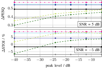
Figure 1: PESQ and STOI improvements for the considered enhancement algorithms in dependence of the peak level of the clean speech signal averaged over all noise types at an input SNR of 0 dB.

To demonstrate the scale-invariance of the proposed features, the considered enhancement approaches are evaluated on speech material where the peak level of the speech utterances is varied systematically. For this, we set the peak level of the speech utterances to $-6~{}\text{dB}$, $-12~{}\text{dB}$, $-18~{}\text{dB}$, $-24~{}\text{dB}$ and $-40~{}\text{dB}$. The $-40~{}\text{dB}$ peak level has not been seen during training and can be considered an extreme case whereas the remaining levels are within the range of variations included in the training data. For this evaluation, the SNR of the input signals is fixed at $-5~{}\text{dB}$ for STOI and $5~{}\text{dB}$ for PESQ. A lower SNR is used for STOI because the speech intelligibility reduces only considerably for SNR lower than $0~{}\text{dB}$. The results in terms of PESQ and STOI improvements are depicted in Fig. 1. For this, the averages over all noise types excluding the CSNE [45] are computed. The results show that the non-ML based speech enhancement algorithms and the ML based approaches based on the normalized features yield the same outcome independent of the scaling of the input signal. Contrarily, the performance of the ML based enhancement scheme using noisy log-spectra varies over the peak level of the input signal. The same can be observed for the combination with the estimated noise PSD. This indicates that by using the normalized features, the ML based algorithm does not depend on the overall level. Contrarily, despite the efforts taken to increase the scale-independence during the training process, the non-normalized features result in scale-dependent results.

The convergence speed of the proposed features is measured using the number of epochs that have been required until the validation error converges. Due to the cross-validation setup, nine models are trained for each feature type which allows to average the number of epochs required to train each model. About 28 to 29 epochs are required on average if the non-normalized features are employed, whereas only 20 to 23 iterations are required for the normalized features. This result provides evidence that the proposed normalized features simplify the training of the respective DNN.

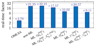
Figure 2: Computational complexity of the considered algorithms in terms of the real-time factor. This factor describes how many seconds of the audio material can be processed within a second in the real world. The number on top of the bar shows the actual value of the real-time factor.

Last, the computational complexity of the considered algorithms is considered. Fig. 2, shows the processing speed of the various algorithms in terms of the real-time factor. The factor describes how many seconds of the audio signal can be processed within a second in the real world. Correspondingly, if the factor is larger than one, the algorithm processes the signals faster than real-time and if the factor is smaller than one, the processing is slower than real-time. The algorithms have been evaluated on the CPU (Intel Core i7-5930K) of a desktop PC. For this, their respective Python or Matlab implementations have been used. Fig. 2 shows that the OMLSA runs slowest while the non-ML described in Section II and the ML based algorithms where the noisy log-spectra ${y}^{\text{(log)}}_{{k,\ell}}$ or the a posteriori SNR $\gamma_{{k,\ell}}$ are used as input feature run fastest. On the used hardware, the quickest algorithms run roughly 20 times faster than real-time. The OMLSA is only about three times faster than real-time which may be explained by the fact that the Matlab implementation is run through Python which potentially introduces further processing overhead. Using the a priori SNR $\xi^{\text{(log)}}_{{k,\ell}}$ instead of the a posteriori $\gamma^{\text{(log)}}_{{k,\ell}}$ reduces the real-time factor to 10. This is because, in comparison to $\gamma^{\text{(log)}}_{{k,\ell}}$, the cepstral smoothing given in Section II-C needs to be additionally computed to obtain $\xi^{\text{(log)}}_{{k,\ell}}$. Using both, the a priori SNR $\xi^{\text{(log)}}_{{k,\ell}}$ and the a posteriori SNR $\gamma^{\text{(log)}}_{{k,\ell}}$, as input features, the real-time factor further drops to 9. Concatenating ${y}^{\text{(log)}}_{{k,\ell}}$ and $\Lambda^{n,\text{(log)}}_{k,\ell}$ is computationally more complex than using the ${Y}_{{k,\ell}}$ normalized by $\Lambda^{n}_{k,\ell}$, i.e., $\gamma^{\text{(log)}}_{{k,\ell}}$. For the concatenated features, the input dimensionality is twice as large as for the a posteriori SNR $\gamma^{\text{(log)}}_{{k,\ell}}$ which results in the additional computational complexity. From this, it is followed that the inclusion of the noise PSD generally increases the computational complexity as expected. Using $\gamma^{\text{(log)}}_{{k,\ell}}$, the increase is only small whereas including the a priori SNR considerably increases the complexity.

IV-C Comparisons

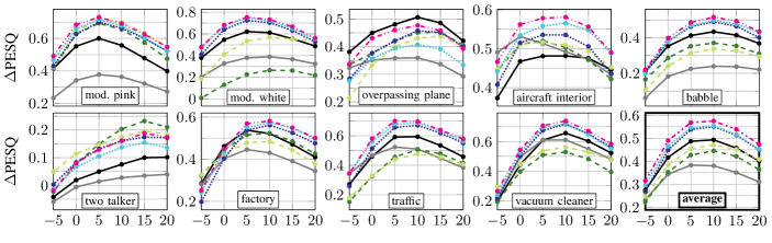
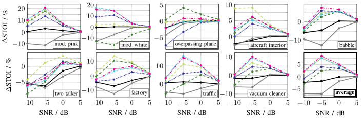
Figure 3: PESQ and STOI improvements that results for the considered enhancement algorithms in dependence of the background noise type and the SNR. The ML based algorithms are always trained on CSNE [45] and the noise types not given in the respective plot, i.e., the background noise is unseen in all cases.

The following results show the outcome of the cross-validation procedure and are used to compare the enhancement algorithms used in this paper. For these experiments, the peak level of the 128 TIMIT sentences used for testing is randomly varied between $-6~{}\text{dB}$ and $-26~{}\text{dB}$ which is similar to the range used for training. Fig. 3 depicts the results.

For both instrumental measures, first the performance of the non-ML based approach is considered. For the aircraft interior noise, the OMLSA achieves higher PESQ scores in low SNR. This is, however, an exception as for the remaining noise types, especially the nonstationary ones such as babble noise or the amplitude modulated versions of the pink and white noise, the performance of the employed non-ML enhancement approach is higher than for the OMLSA. In terms of the speech intelligibility predicted by STOI, both non-ML approaches have either little effect or reduce the intelligibility. In all cases, however, $\Delta$STOI is higher for the approach described in Section II than for the OMLSA. Consequently, the algorithm described in Section II generally outperforms the OMLSA [4, 5].

The speech intelligibility predicted by STOI is generally higher for the ML based algorithms than for the non-ML approaches. In factory noise and the aircraft interior noise, STOI predicts a higher speech intelligibility for the non-normalized features. The same is true for the overpassing plane and the two-talker noise. Here, however, $\Delta$STOI is generally smaller compared to the other noise types. Among the non-normalized features, $\Delta$STOI is generally higher for the combination of the noisy log-spectra ${y}^{\text{(log)}}_{{k,\ell}}$ and the estimated noise PSD $\Lambda^{n,\text{(log)}}_{k,\ell}$. For the remaining noise types, however, the proposed normalized features yield similar or higher STOI improvements than the non-normalized features. Comparing the normalized feature sets amongst each other shows that using only the a priori SNR $\xi^{\text{(log)}}_{{k,\ell}}$ often results in the lowest scores. Contrarily, the combination of the a priori SNR $\xi^{\text{(log)}}_{{k,\ell}}$ and the a posteriori SNR $\gamma^{\text{(log)}}_{{k,\ell}}$ generally yields the highest scores. In many cases, using only the a posteriori SNR $\gamma^{\text{(log)}}_{{k,\ell}}$ yields scores similar to the combination. For cases, where the computational complexity plays an important role this feature type is thus a considerable alternative.

The PESQ improvements for the ML based algorithms indicate a clear preference for the proposed normalized features. Only for the two talker noise, the PESQ improvements obtained for the non-normalized features are higher than for the normalized features. However, as basically all the considered enhancement algorithms struggle in this noise type, the gains of 0.05 points are rather small and therefore negligible. For most of the remaining noise types, the performance of the non-normalized features predicted by PESQ is between the OMLSA and the non-ML approach described in Section II. Except for the modulated white noise, PESQ does not indicate considerable advantages if an estimate of the noise PSD $\Lambda^{n,\text{(log)}}_{k,\ell}$ is appended to the noisy log-spectra ${y}^{\text{(log)}}_{{k,\ell}}$. This changes if the normalized features are used. Using these features, the performance of the ML approach is more robust and, often, both non-ML approaches are outperformed. Again, the combination of the a priori SNR $\xi^{\text{(log)}}_{{k,\ell}}$ and a posteriori SNR $\gamma^{\text{(log)}}_{{k,\ell}}$ yields the highest scores in most noise types. Also here, using the a posteriori SNR $\gamma^{\text{(log)}}_{{k,\ell}}$ without the a priori SNR $\xi^{\text{(log)}}_{{k,\ell}}$ yields similar results as the combination of both. Consequently, it is possible to benefit from the advantages of the normalized features without severely increasing the computational complexity. Further, as this feature type has the same dimensionality as the noisy log-spectra, this demonstrates the importance of the normalized features on the generalization of ML based enhancement schemes.

V Subjective Evaluation

Instrumental measures such as PESQ give an indication on how the quality of the processed signals would be judged by humans. Still, as such measures cannot perfectly model human perception, we verify the instrumental results in Section IV using subjective evaluation tests. Here, a MUSHRA [49] is employed to compare the algorithms described in Section II and Section III. First, the audio material, parameters and evaluation are explained and, after that, the results are discussed.

V-A Audio Material, Parameters and Setup

For this experiment, a sentence of a male and a female speaker is embedded in factory 1 noise and traffic noise at an SNR of 5 dB. The noisy signals are processed by the speech enhancement schemes described in Section II and Section III. The ML based algorithm is included once using the noisy log-spectra as features ${y}^{\text{(log)}}_{{k,\ell}}$ and once using the combination of a priori SNR $\xi^{\text{(log)}}_{{k,\ell}}$ and a posteriori SNR $\gamma^{\text{(log)}}_{{k,\ell}}$. For this experiment, the CSNE [45] and the two talker noise are excluded from the noise type pool such that eight noise types remain. We train the DNN once on a set which includes mod. pink noise, mod. white noise, factory 1 noise and traffic noise. Note that this includes the traffic and factory noise which is also used for testing, i.e., this corresponds to a seen condition. For this condition, it is ensured that the noise realizations used for the training are not reused for testing. Therefore, only the first $120~{}\text{s}$ of the noise types are used while the last $120~{}\text{s}$ are used to embed the sentences for the listening experiment. The algorithms have also been evaluated in an unseen condition where all noise types are included in the training set except the one used for evaluation. Here, the full length of the training noise is utilized. For each sentence embedded in the training noise type, the peak level is varied between $-26~{}\text{dB}$ and $-6~{}\text{dB}$, while the SNR is chosen between $-5~{}\text{dB}$ and $15~{}\text{dB}$. The minimum gain is set to $G_{\text{min}}=-15~{}\text{dB}$ in this experiment.

In each trial of the experiment, the participants compared six stimuli. In addition to the processed signals, the noisy signal is included and a reference signal is presented where the speech signal and the background noise are mixed at an SNR of $20~{}\text{dB}$. Lastly, a low quality anchor is added where the speech signal is low pass filtered at $2~{}\text{kHz}$ and mixed at an SNR of $-5~{}\text{dB}$. This signal is enhanced using a non-ML based enhancement algorithm where the noise PSD is estimated using [9] while the speech PSD is obtained using the decision-directed approach [2]. The smoothing constant is set to $0.9$ and the signal is enhanced using the Wiener filter where a more aggressive lower limit of $-20~{}\text{dB}$ is employed. This results in an anchor signal with very poor quality due to many musical tone artifacts and strong speech distortions. The audio examples used for the listening experiment are available under https://www.inf.uni-hamburg.de/en/inst/ab/sp/publications/tasl2017-dnn-rr.

A total of 11 subjects with age in the range of 24 to 38 years who are not familiar with single-channel signal processing have participated in the MUSHRA. The experiment took place in a quiet office. The diotic signals were presented via Beyerdynamic DT-770 Pro 250 Ohm headphones attached to an RME Fireface UFX+ sound card. All signals were normalized in amplitude. The test consisted of two phases. First, the participants were asked to complete a training phase to familiarize with the presented sounds and to adjust the volume to a comfortable level. For this, a subset of the processed signals was presented. In the second part of the experiment, the participants were asked to rate the signals according to their overall preference on a scale from 0 to 100, where 0 was labeled with “bad” and 100 with “excellent”. The order of the presentation of algorithms and conditions were randomized between all subjects.

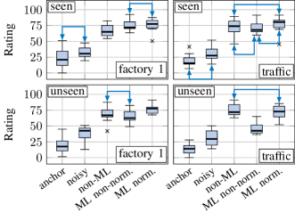
Figure 4: Box plots for the subjective rating of different enhancement schemes. The left column shows the results for factory 1 noise and the right column for traffic noise as test signals. The rows show different training strategies. The linking lines show pairings that are not identified as statistically significant by the post-hoc tests.

V-B Results

For the evaluation, we average the ratings over the two speakers for each tested scenario. Further, the results are validated using a statistical analysis. For each acoustic scenario, a repeated measures ANOVA [50] is performed to test if the factor “enhancement algorithm” has a significant effect on the participants’ rating. For this, we employ a significance level of 5 % for all statistical tests. For each acoustic scenario, we validated that the residuals of the general linear model fitted during the process of the repeated measures ANOVA are normally distributed using the Shapiro-Wilk test [51]. The sphericity assumption has been validated using Mauchly’s test [52] and a Greenhouse-Geisser correction [53] is employed in cases where it has been violated. In all acoustic scenarios, the enhancement algorithms have a statistically significant effect on ratings. Hence, post-hoc tests are used to identify the sources of significance. For this, matched pair $t$-tests with a Bonferroni-Holm [54] correction are employed to account for the error inflation. The results are shown in Fig. 4 where the ratings that are statistically not significantly different are indicated by linking lines.

All listeners were able to correctly identify the hidden reference and assigned the highest score to it. The anchor signal and the noisy signal were assigned the lowest scores in most of the cases. For the seen conditions, all enhancement schemes have been rated similar in traffic noise, while in factory noise, both ML based speech enhancement schemes yield slightly better results than the non-ML based algorithm. For the unseen conditions, the ratings for the ML based approach only using the non-normalized noisy log-spectra as features drop while the ratings for the proposed normalized features remain high. Additionally, the proposed features show slightly higher ratings in comparison to the non-ML enhancement scheme in factory noise. The statistical evaluation confirms that the highlighted differences are statistically significant.

VI Conclusions

In this paper, we propose features for ML based speech enhancement which incorporate non-ML based estimates of the speech and noise PSD. The goal is to improve the robustness of ML based enhancement scheme towards unseen noise conditions. In contrast to the already existing noise aware training [36, 37, 12, 35], the noise PSD is not appended but used as a normalizing term. This results in the a priori SNR and the a posteriori SNR which exhibit the advantageous property of being scale-invariant. For the noisy log-spectra, the performance of the ML based enhancement scheme in terms of PESQ is low in unseen noise conditions. Appending an estimate of the noise PSD has only a little impact on the performance in PESQ while the intelligibility predicted by STOI increases. Using the proposed normalized features, however, the performance of the ML based enhancement scheme is generally higher as for the compared algorithms in both instrumental measures. This is supported by the MUSHRA based listening experiments where, in unseen noise conditions, the proposed combination was significantly preferred over the ML based enhancement scheme using only the log-spectra of the noisy observations. Audio examples are available under https://www.inf.uni-hamburg.de/en/inst/ab/sp/publications/tasl2017-dnn-rr. Feed-forward networks clearly benefit from the proposed normalized features, but their effect on other architectures such as recurrent neural networks or convolutional networks remains a question for future research.

References

- [1] P. Vary and R. Martin, Digital speech transmission: Enhancement, Coding and Error Concealment. Chichester, West Sussex, UK: Wiley & Sons, 2006.
- [2] Y. Ephraim and D. Malah, “Speech Enhancement Using a Minimum-Mean Square Error Short-Time Spectral Amplitude Estimator,” IEEE Transactions on Acoustics, Speech, and Signal Processing, vol. 32, no. 6, pp. 1109–1121, Dec. 1984.
- [3] Y. Ephraim, “A Bayesian Estimation Approach for Speech Enhancement Using Hidden Markov Models,” IEEE Transactions on Signal Processing, vol. 40, no. 4, pp. 725–735, Apr. 1992.
- [4] I. Cohen and B. Berdugo, “Speech enhancement for non-stationary noise environments,” Signal Processing, vol. 81, no. 11, pp. 2403–2418, 2001.
- [5] I. Cohen, “Noise spectrum estimation in adverse environments: improved minima controlled recursive averaging,” IEEE Transactions on Speech and Audio Processing, vol. 11, no. 5, pp. 466–475, Sep. 2003.
- [6] S. Srinivasan, J. Samuelsson, and W. B. Kleijn, “Codebook Driven Short-Term Predictor Parameter Estimation for Speech Enhancement,” IEEE Transactions on Audio, Speech, and Language Processing, vol. 14, no. 1, pp. 163–176, Jan. 2006.
- [7] D. Y. Zhao and W. B. Kleijn, “HMM-Based Gain Modeling for Enhancement of Speech in Noise,” IEEE Transactions on Audio, Speech, and Language Processing, vol. 15, no. 3, pp. 882–892, Mar. 2007.
- [8] C. Breithaupt, T. Gerkmann, and R. Martin, “A novel a priori SNR estimation approach based on selective cepstro-temporal smoothing,” in IEEE International Conference on Acoustics, Speech and Signal Processing (ICASSP), Las Vegas, NV, USA, Apr. 2008, pp. 4897–4900.
- [9] T. Gerkmann and R. C. Hendriks, “Noise Power Estimation Based on the Probability of Speech Presence,” in IEEE Workshop on Applications of Signal Processing to Audio and Acoustics (WASPAA), New Paltz, NY, USA, 2011, pp. 145–148.
- [10] ——, “Unbiased MMSE-Based Noise Power Estimation With Low Complexity and Low Tracking Delay,” IEEE Transactions on Audio, Speech, and Language Processing, vol. 20, no. 4, pp. 1383–1393, May 2012.
- [11] N. Mohammadiha, P. Smaragdis, and A. Leijon, “Supervised and Unsupervised Speech Enhancement Using Nonnegative Matrix Factorization,” IEEE Transactions on Audio, Speech, and Language Processing, vol. 21, no. 10, pp. 2140–2151, Oct. 2013.
- [12] Y. Xu, J. Du, L. R. Dai, and C. H. Lee, “A Regression Approach to Speech Enhancement Based on Deep Neural Networks,” IEEE/ACM Transactions on Audio, Speech, and Language Processing, vol. 23, no. 1, pp. 7–19, Jan. 2015.
- [13] S. E. Chazan, J. Goldberger, and S. Gannot, “A Hybrid Approach for Speech Enhancement Using MoG Model and Neural Network Phoneme Classifier,” IEEE/ACM Transactions on Audio, Speech, and Language Processing, vol. 24, no. 12, pp. 2516–2530, Dec. 2016.
- [14] Y. Ephraim and D. Malah, “Speech Enhancement Using a Minimum Mean-Square Error Log-Spectral Amplitude Estimator,” IEEE Transactions on Acoustics, Speech, and Signal Processing, vol. 33, no. 2, pp. 443–445, 1985.
- [15] R. Martin, “Noise Power Spectral Density Estimation Based on Optimal Smoothing and Minimum Statistics,” IEEE Transactions on Speech and Audio Processing, vol. 9, no. 5, pp. 504–512, Jul. 2001.
- [16] C. Breithaupt, M. Krawczyk, and R. Martin, “Parameterized MMSE Spectral Magnitude Estimation for the Enhancement of Noisy Speech,” in IEEE International Conference on Acoustics, Speech and Signal Processing (ICASSP), Las Vegas, NV, USA, Apr. 2008, pp. 4037–4040.
- [17] R. C. Hendriks, T. Gerkmann, and J. Jensen, DFT-Domain Based Single-Microphone Noise Reduction for Speech Enhancement: A Survey of the State of the Art, ser. Synthesis Lectures on Speech and Audio Processing. Morgan & Claypool Publishers, 2013, vol. 9, no. 1.
- [18] D. Burshtein and S. Gannot, “Speech Enhancement Using a Mixture-Maximum Model,” IEEE Transactions on Speech and Audio Processing, vol. 10, no. 6, pp. 341–351, Sep. 2002.
- [19] Y. Wang, A. Narayanan, and D. Wang, “On Training Targets for Supervised Speech Separation,” IEEE/ACM Transactions on Audio, Speech, and Language Processing, vol. 22, no. 12, pp. 1849–1858, Dec. 2014.
- [20] J. Chen, Y. Wang, S. E. Yoho, D. Wang, and E. W. Healy, “Large-scale training to increase speech intelligibility for hearing-impaired listeners in novel noises,” The Journal of the Acoustical Society of America, vol. 139, no. 5, pp. 2604–2612, 2016.
- [21] Q. He, F. Bao, and C. Bao, “Multiplicative Update of Auto-Regressive Gains for Codebook-Based Speech Enhancement,” IEEE/ACM Transactions on Audio, Speech, and Language Processing, vol. 25, no. 3, pp. 457–468, Mar. 2017.
- [22] M. Kolbæk, Z. H. Tan, and J. Jensen, “Speech Intelligibility Potential of General and Specialized Deep Neural Network Based Speech Enhancement Systems,” IEEE/ACM Transactions on Audio, Speech, and Language Processing, vol. 25, no. 1, pp. 149–163, Jan. 2017.
- [23] S. Suhadi, C. Last, and T. Fingscheidt, “A Data-Driven Approach to A Priori SNR Estimation,” IEEE Transactions on Audio, Speech, and Language Processing, vol. 19, no. 1, pp. 186–195, Jan. 2011.
- [24] B. Xia and C. Bao, “Wiener filtering based speech enhancement with Weighted Denoising Auto-encoder and noise classification,” Speech Communication, vol. 60, no. Supplement C, pp. 13–29, May 2014.
- [25] A. Chinaev, J. Heymann, L. Drude, and R. Haeb-Umbach, “Noise-Presence-Probability-Based Noise PSD Estimation by Using DNNs,” in ITG Conference on Speech Communication, Paderborn, Germany, Oct. 2016.
- [26] F. Weninger, J. R. Hershey, J. Le Roux, and B. Schuller, “Discriminatively Trained Recurrent Neural Networks for Single-Channel Speech Separation,” in IEEE Global Conference on Signal and Information Processing (GlobalSIP), Atlanta, GA, USA, Dec. 2014, pp. 577–581.
- [27] X. Lu, Y. Tsao, S. Matsuda, and C. Hori, “Speech Enhancement Based on Deep Denoising Autoencoder,” in Conference of the International Speech Communication Association (Interspeech), Lyon, France, Aug. 2013.
- [28] A. L. Maas, Q. V. Le, T. M. O’Neil, O. Vinyals, P. Nguyen, and A. Y. Ng, “Recurrent Neural Networks for Noise Reduction in Robust ASR,” in Conference of the International Speech Communication Association (Interspeech), Portland, OR, USA, Sep. 2012, pp. 22–25.
- [29] F. Weninger, F. Eyben, and B. Schuller, “Single-channel speech separation with memory-enhanced recurrent neural networks,” in IEEE International Conference on Acoustics, Speech and Signal Processing (ICASSP), May 2014, pp. 3709–3713.
- [30] S. R. Park and J. W. Lee, “A Fully Convolutional Neural Network for Speech Enhancement,” in Conference of the International Speech Communication Association (Interspeech). Stockholm, Sweden: ISCA, Aug. 2017, pp. 1993–1997.
- [31] S. Pascual, A. Bonafonte, and J. Serrà, “SEGAN: Speech Enhancement Generative Adversarial Network,” in Conference of the International Speech Communication Association (Interspeech), Aug. 2017, pp. 3642–3646.
- [32] D. Michelsanti and Z.-H. Tan, “Conditional Generative Adversarial Networks for Speech Enhancement and Noise-Robust Speaker Verification,” in Conference of the International Speech Communication Association (Interspeech), Stockholm, Sweden, Aug. 2017, pp. 2008–2012.
- [33] A. van den Oord, S. Dieleman, H. Zen, K. Simonyan, O. Vinyals, A. Graves, N. Kalchbrenner, A. Senior, and K. Kavukcuoglu, “WaveNet: A Generative Model for Raw Audio,” arXiv:1609.03499 [cs], Sep. 2016, arXiv: 1609.03499. [Online]. Available: http://arxiv.org/abs/1609.03499
- [34] K. Qian, Y. Zhang, S. Chang, X. Yang, D. Florêncio, and M. Hasegawa-Johnson, “Speech Enhancement Using Bayesian Wavenet,” in Proc. Interspeech 2017, Aug. 2017, pp. 2013–2017.
- [35] A. Kumar and D. Florencio, “Speech Enhancement in Multiple-Noise Conditions Using Deep Neural Networks,” in Conference of the International Speech Communication Association (Interspeech), San Francisco, CA, USA, Sep. 2016, pp. 3738–3742.
- [36] M. L. Seltzer, D. Yu, and Y. Wang, “An investigation of deep neural networks for noise robust speech recognition,” in IEEE International Conference on Acoustics, Speech and Signal Processing (ICASSP), Vancouver, BC, Canada, May 2013, pp. 7398–7402.
- [37] Y. Xu, J. Du, L.-R. Dai, and C.-H. Lee, “Dynamic Noise Aware Training for Speech Enhancement Based on Deep Neural Networks,” in Conference of the International Speech Communication Association (Interspeech), Singapore, Singapore, Sep. 2014.
- [38] “P.862: Perceptual evaluation of speech quality (PESQ): An objective method for end-to-end speech quality assessment of narrow-band telephone networks and speech codecs,” International Telecommunication Union, ITU-T recommendation, Jan. 2001. [Online]. Available: http://www.itu.int/rec/T-REC-P.862-200102-I/en
- [39] C. H. Taal, R. C. Hendriks, R. Heusdens, and J. Jensen, “An Algorithm for Intelligibility Prediction of Time-Frequency Weighted Noisy Speech,” IEEE Transactions on Audio, Speech, and Language Processing, vol. 19, no. 7, pp. 2125–2136, Sep. 2011.
- [40] M. Berouti, R. Schwartz, and J. Makhoul, “Enhancement of speech corrupted by acoustic noise,” in IEEE International Conference on Acoustics, Speech, and Signal Processing (ICASSP), Washington, D.C., USA, Apr. 1979, pp. 208–211.
- [41] D. Brillinger, Time Series - Data Analysis and Theory, ser. Classics in Applied Mathematics. Society for Industrial and Applied Mathematics, Jan. 2001.
- [42] T. Gerkmann and R. Martin, “On the Statistics of Spectral Amplitudes After Variance Reduction by Temporal Cepstrum Smoothing and Cepstral Nulling,” IEEE Transactions on Signal Processing, vol. 57, no. 11, pp. 4165–4174, 2009.
- [43] V. Nair and G. E. Hinton, “Rectified Linear Units Improve Restricted Boltzmann Machines,” in International Conference on Machine Learning, Haifa, Israel, Jun. 2010, pp. 807–814.
- [44] H. J. M. Steeneken and F. W. M. Geurtsen, “Description of the RSG.10 noise database,” TNO Institute for perception, Technical Report IZF 1988-3, 1988.
- [45] G. Hu, “A corpus of nonspeech sounds.” [Online]. Available: http://web.cse.ohio-state.edu/pnl/corpus/HuNonspeech/HuCorpus.html
- [46] J. S. Garofolo, L. F. Lamel, W. M. Fisher, J. G. Fiscus, D. S. Pallett, N. L. Dahlgren, and V. Zue, “TIMIT Acoustic-Phonetic Continuous Speech Corpus,” 1993.
- [47] X. Glorot and Y. Bengio, “Understanding the difficulty of training deep feedforward neural networks,” in International Conference on Artificial Intelligence and Statistics (AISTATS), Chia Laguna Resort, Sardinia, Italy, May 2010, pp. 249–256.
- [48] J. C. Duchi, E. Hazan, and Y. Singer, “Adaptive Subgradient Methods for Online Learning and Stochastic Optimization,” Journal of Machine Learning Research, vol. 12, pp. 2121–2159, 2011.
- [49] “BS.1534-3: Method for the subjective assessment of intermediate quality levels of coding systems,” International Telecommunication Union, ITU-T recommendation, Oct. 2015. [Online]. Available: http://www.itu.int/rec/R-REC-BS.1534-3-201510-I/en
- [50] A. Field, Disocvering Statistics Using SPSS, 3rd ed. SAGE Publications Ltd., 2009.
- [51] S. S. Shapiro and M. B. Wilk, “An Analysis of Variance Test for Normality (Complete Samples),” Biometrika, vol. 52, no. 3/4, pp. 591–611, 1965.
- [52] J. W. Mauchly, “Significance Test for Sphericity of a Normal n-Variate Distribution,” The Annals of Mathematical Statistics, vol. 11, no. 2, pp. 204–209, Jun. 1940.
- [53] S. W. Greenhouse and S. Geisser, “On methods in the analysis of profile data,” Psychometrika, vol. 24, no. 2, pp. 95–112, Jun. 1959.
- [54] S. Holm, “A Simple Sequentially Rejective Multiple Test Procedure,” Scandinavian Journal of Statistics, vol. 6, no. 2, pp. 65–70, 1979.