Comment on the MS ”Null weak values and the past of quantum particle” by Q.Duprey and A.Matzkin

Abstract

In a recent paper Matz , Duprey and Matzin investigeated the meaning of vanishing ”weak values” (WV), and their role in the retrodiction of the past of a pre- and post-selected quantum system in the presence of interference. Here we argue that any proposition, regarding the WV values, should be understood as a statement about the probability amplitudes, and revisit some of the conclusions reached in Matz .

Keywords; quantum particle’s past, transition amplitudes, weak measurements

I Introduction

In a recent publication Matz , Duprey and Matzin analysed physical significance of the vanishing weak values. They also commented on our related work PLA2017 , suggesting that its approach ” discards any possibility to infer a property from protocols implementing nondestructive weak interactions.” Here we clarify our position on the issue, and discuss some of the conclusions arrived at in Matz . We start with the basics.

Standard quantum mechanics postulates the existence of probability amplitudes, whose evaluation inevitably precedes the calculation of probabilities, related to the frequencies with which physical phenomena are observed. The amplitudes are complex valued quantities with no specific prescription for the signs of their real and imaginary parts. The rules for using them are well known (see, for example, the three points of the Summary on the page 1-10 of Feynl ). Any ”deeper meaning” these axiomatic quantities might have is not available to us. Feynman’s statement that ”we have no ideas about a more basic mechanism…” Feynl remains, we argue, valid to this day.

II Virtual pathways and functionals

As the first point, we note next that our analysis need not be limited to quantities represented by hermitian operators, so that the ”eigenstate-eigenvalue link” often mentioned in Matz is of no particular importance to us. Consider a system going from $|\psi_{I}{\rangle}$ at $t_{1}$ to $|\psi_{F}{\rangle}$ at $t_{2}$ via $N$ alternative ways (pathways, paths), $\{i\}$, $i=1,2,..,N$, each endowed with the probability amplitude $A^{F\leftarrow I}_{i}$. To distinguish between the pathways, we may employ a functional $F$, taking a real value $\mathcal{F}_{i}$ on the $i$-th path,

$$F[i]=\sum_{i}\mathcal{F}_{j}F^{j}[i],\quad F^{j}[i]=\delta_{ij},$$ (1)

where $\delta_{ij}$ is the Kronecker delta. As a simple example, consider an $F$ representing the difference between the values of an operator $\hat{B}$ at some intermediate times $t^{\prime}$ and $t^{\prime\prime}$. In a two dimensional Hilbert space $\mathcal{H}$, and for a $\hat{B}$ with eigenvalues of $\pm 1$, the said difference can take three distinct values of $2$, $0$, and $-2$. It is clear that a measurement of $F$ cannot be reduced to projecting onto the eigenstates of an operator, since no operator acting in $\mathcal{H}$ can have more than two different eigenvalues DSMath . Other examples of functionals referring to more than one moment in time, include the residence time of a qubit QRES , time average of a dynamical variable TIMAV , and the quantum traversal time QTT .

III Accurate (strong) measurements with post-selection

In can be shown DSMath that if $K\leq N$ of the $\mathcal{F}$s are different, an accurate (strong) meter would destroy interference between the unions (superpositions DSMath ) of paths corresponding to the different values of $F$. It will, therefore, create $K$ exclusive routes Feynl endowed with both the amplitudes [$\Delta(a-b)=1$ for $a=b$, and $0$ otherwise]

$$\tilde{A}^{F\leftarrow I}_{k}=\sum_{i=1}^{N}A^{F\leftarrow I}_{i}\Delta(\mathcal{F}_{i}-\mathcal{F}_{k}),\quad k=1,2,...,K,$$ (2)

and the probabilities $P^{F\leftarrow I}_{k}=|\tilde{A}^{F\leftarrow I}_{k}|^{2}$ An accurate pointer would always point at one of the $\mathcal{F}_{k}$, so that for its mean shift we have

$${\langle}f{\rangle}_{s}=\sum_{i=1}^{K}\mathcal{F}_{k}P^{F\leftarrow I}_{k}/\sum_{j=1}^{K}P^{F\leftarrow I}_{j}.$$ (3)

Importantly, Eq.(2) is a statement about the probabilities $P^{F\leftarrow I}_{k}$, created by our accurate meter. Namely, we learn that multiplying them by $\mathcal{F}_{k}$, and adding up the products, would yield the number in the l.h.s. of Eq.(2). If we can accurately measure a functional $F_{M}[i]$ taking the value of $1$ on, say, the first $M$ paths and $0$ on the rest of them, Eq.(3), with $K=2$, will yield the probability for travelling the exclusive (real) route, given by superposition of the said $M$ paths.

IV Inaccurate (weak) measurements with post-selection

On the other hand, an inaccurate (weak) meter would perturb the system only slightly, and not create probabilities for individual pathways, or their unions. The ”weakness” can be achieved by either reducing the coupling to the meter, or by broadening the initial pointer state in the coordinate space (see Sect. 10 of PLA2015 ). It is easy to show Ah1 , DSMath that the mean pointer shift may be given by

$${\langle}f{\rangle}_{w}=\text{Re}(\text{Im})\left[\sum_{k}\mathcal{F}_{k}\tilde{\alpha}^{F\leftarrow I}_{k}\right],\quad\tilde{\alpha}^{F\leftarrow I}_{k}\equiv\frac{\tilde{A}^{F\leftarrow I}_{k}}{\sum_{j=1}^{K}\tilde{A}^{F\leftarrow I}_{j}},\quad$$ (4)

where the choice of the real or imaginary part depends on how the measurement is set up Ah1 , DSMath . In the absence of probabilities, Eq.(4) is a statement about the (relative) probability amplitudes $\tilde{\alpha}^{F\leftarrow I}_{k}$. Multiplying them by $\mathcal{F}_{k}$, adding them up, and taking the real (imaginary) parts, would yield the number in the l.h.s. of Eq.(4). A weak measurement of the $F_{M}[i]$, mentioned above, will yield the amplitude for the pathway uniting the first $M$ paths.

V Null weak value of a projector

The general principle just outlined, applies also to the particular case studied in Matz . Now the quantity of interest is the instantaneous value of an operator $\hat{B}=\sum_{i=1}^{N}|b_{i}{\rangle}B_{i}{\langle}b_{i}|$, with the eigenstates $|b_{i}{\rangle}$ and eigenvalues $B_{i}$, evaluated at some $t_{1}<t<t_{2}$. In general, $K\leq N$ of the eigenvalues $B_{i}$ may be different. We, therefore, have

$$.\mathcal{F}_{k}=B_{k},\quad\text{and}\quad\quad\quad\quad\quad\quad\quad$$ (5)

$$\tilde{A}^{F\leftarrow I}_{k}=\sum_{i=1}^{N}{\langle}\psi_{F}|\hat{U}(t_{2},t)|b_{i}{\rangle}{\langle}b_{i}|\hat{U}(t,t_{1})|\psi_{I}{\rangle}\Delta(B_{i}-B_{k}),$$

where $\hat{U}(t_{2},t)$ is the system’s evolution operator.
Following Ref. Matz , we first look at a ”null weak value of a projecting operator”, $K=2$, and $B_{k}=\delta_{km}$. In agreement with the above, the authors of Matz note that a weak measurement of this projector ”picks up a relative path amplitude”, $\tilde{\alpha}^{F\leftarrow I}_{m}={\langle}\psi_{F}|\hat{U}(t_{2},t)|b_{m}{\rangle}{\langle}b_{m}|\hat{U}(t,t_{1})|\psi_{I}{\rangle}/{\langle}\psi_{F}|\hat{U}(t_{2},t_{1})|\psi_{I}{\rangle}$, which, in this case, happens to be zero. They proceed, however, to conclude that ”it is meaningless to make any assertion concerning the property of the system if interferences are not lifted by a strong coupling”. This is not our position. The probability amplitudes are well defined quantities in quantum mechanics. They are particular properties of a pre- and post-selected quantum system Feynl , and we just found one of them to be zero. We argue that little else can be added to this conclusion. The main achievement of the ”weak measurement theory” (for a review see WMrev ) is the discovery of a scheme whereby the response of a weakly perturbed system yields the value of the amplitude in question. Its main problem is not recognising the amplitude for what they are PLA2016 , DSEA .

VI An amplitude is just an amplitude

One may take a view that the only ”physical” quantities are the probabilities and the average values of the observed quantities. The amplitudes, on the other hand, should be just computational tools, no longer needed once the calculation is completed. Is it then surprising that the values of these theoretical constructs can be determined in an experiment? We argue that it is not. Like the probability itself, a probability amplitude characterises an ensemble. A probability cannot be measured directly in a single attempt, and requires many trials for the frequency, with which the $i$-th property appears, to approach the probability $P(i)=|A(i)|^{2}$. But by the time $P(i)$ is evaluated, we will have measured indirectly also the modulus of the amplitude $A(i)$, $|A(i)|=\sqrt{P(i)}$. Furthermore, a small perturbation applied to the system would change $A(i)$ by $\delta A(i)$, and the probability $P(i)$ by $\delta P(i)\approx 2Re[A(i)\delta A(i)]$. Thus, comparing the perturbed and unperturbed frequencies we can indirectly measure the real part of a complex valued quantity $A(i)\delta A(i)$. Similarly, in a weak measurement of a projector, many accurate observations of the pointer’s position, allow us to deduce the value of $\text{Re}\left[\alpha^{F\leftarrow I}_{i}\right]$. One’s ability to measure probability amplitudes indirectly is a trivial consequence of the perturbation theory and the structure of quantum probabilities. However, such measurements provide no deeper insight into their physical meaning. The amplitudes remain just something one needs to square in order to arrive at observable frequencies, in other words, the probability amplitudes.

VII ”Weak traces” and interferometers

In a nutshell, the case of the ”three-path interferometer” discussed in Matz involves three pathways with $A^{F\leftarrow I}_{i}\neq 0$, of which two amplitudes have equal magnitudes, but opposite signs, e.g., $A^{F\leftarrow I}_{1}=-A^{F\leftarrow I}_{2}\neq 0$ (see Fig.1a).

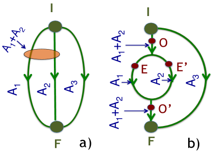
Figure 1: (Color online) a) Three virtual paths with relative amplitudes $A_{i}$, $i=1,2,3$ (we omit the superscript $F\leftarrow I$) connect the initial and the final states of a particle. For $A_{1}=-A_{2}\neq 0$, and $A_{3}\neq 0$, a weak meter would give non-zero readings in the paths $1$ and $2$, but not in their superposition. b) The same system, but with paths $1$ an $2$ merged before and after the inner loop. The weak meter would give non-zero readings at $E$ and $E^{\prime}$, but not at $O$ and $O^{\prime}$, creating an impression that the particle ”was” in the loop ”, yet never entered or exited it”.

Now, from (3), weak measurements of operators $\hat{\Pi}_{1}=|b_{1}{\rangle}{\langle}b_{1}|$ or $\hat{\Pi}_{2}=|b_{2}{\rangle}{\langle}b_{2}|$ would detect an non-zero mean shift of the pointer (a weak trace). One is tempted to conclude that the particle ”was” wherever the traces were left. But then a measurement of the projector on the union of the two paths, $\hat{\Pi}_{1+2}=|b_{1}{\rangle}{\langle}b_{1}|+|b_{2}{\rangle}{\langle}b_{2}|$ would yield no weak trace. All three measurements can be made simultaneously, e.g., by putting the meters at some locations $O$, $E$,$E^{\prime}$ and $O^{\prime}$ (see Fig.1b). So should we conclude that a quantum particle is in the first and second path, but not in their union (superposition) at the same time FOOT ?
The authors of Matz answer the question as follows: ”If the system cannot go through O and be detected in the postselected state, then we can say that ’the particle was not there’ provided ’was’ is employed in a liberal sense because ’the system’ is generally taken to mean ’the system state,’ whereas here we are discerning a particular particle property correlated with a transition to a postselected state.”
Our answer is, however, different. According to (2), a pointer placed at $O$ or $O^{\prime}$ would unite paths $1$ and $2$ in Fig. 1, while leaving path $3$ intact. The amplitude for the combined path $1\cup 2$ is $\tilde{A}^{F\leftarrow I}_{1}=A^{F\leftarrow I}_{1}+A^{F\leftarrow I}_{2}=0$, and a weak measurement at these two locations would yield a null mean shift $\text{Re}[(A^{F\leftarrow I}_{1}+A^{F\leftarrow I}_{2})/\sum_{j=1}^{3}A^{F\leftarrow I}_{j}]=0$. A pointer placed at $E$ would unite paths $2$ and $3$, and yield a nonzero mean shift $\text{Re}[A^{F\leftarrow I}_{1}/A^{F\leftarrow I}_{3}]\neq 0$. Similarly, a non-zero pointer shift will be obtained for a pointer placed at $E^{\prime}$. We have, therefore, obtained the values of the amplitudes for the real pathways that would be created, should a strong meter be applied at $O$, $O^{\prime}$, $E$, or $E^{\prime}$. We argue that the above is the only consistent description offered by conventional quantum mechanics. We refrain from using the notion of a particle ”being there” even in the liberal sense employed by the authors of Matz , in order to avoid inconsistencies and spurious ”paradoxes” that might arise.
One such paradox is the case of a photon passing through a ”nested Mach-Zehnder interferometer” first studied in Vaid , and also discussed in Matz and PLA2017 . There the photon is thought to be ”found” in the nested loop, similar to the one shown in Fig. 1b, but not in the arms leading to and from it F1 . (We stress that this was not the opinion shared by the authors of Matz , who argued instead that the evolving wavefunction physically behaves as an extended object whose properties relative to pre- and post-selected states can be measured locally.) However, accepting the proposition of F1 , one would need to explain also why the photon is no longer ”found” inside the loop if the ingoing arm (where it ”never was”) is blocked DSrepl , so that $A^{F\leftarrow I}_{1}=A^{F\leftarrow I}_{2}=0$. If it is proposed that quantum motion can be affected by something that happens in the region the particle never visits, a further problem would arise. An experiment performed in Los Angeles should not depend on what happens in Paris precisely because the particle stays in the lab, and never visits France. Should then there be two senses in which the particle ”is not there”, one for a particular part of the interferometer, and another for the rest of the world? It would be prudent to stop here. A reasoning which requires ever more assumptions of increasing complexity is unlikely to be helpful, and a recourse to the axioms of the theory Feynl , however restrictive they may seem, should be preferred Russ .

VIII Null weak value of an arbitrary observable

Finally, the authors of Ref.Matz considered the case of ”null weak value of a general observable” where the quantity in the square brackets in Eq.(4) (weak value of an operator $\hat{B}$, denoted $B_{w}$) vanishes for a particular choice of the states $|\psi_{F}{\rangle}$ and $|\psi_{I}{\rangle}$. Assuming, for simplicity, that none of the eigenvalues $B_{i}$ are degenerate, and not all of $\tilde{A}^{F\leftarrow I}_{i}$ vanish, we have

$$B_{w}\equiv\sum_{k}B_{k}\tilde{\alpha}^{F\leftarrow I}_{m}=\frac{{\langle}\psi_{F}|\hat{U}(t_{2},t)\hat{B}\hat{U}(t,t_{1})|\psi_{I}{\rangle}}{{\langle}\psi_{F}|\hat{U}(t_{2},t_{1})|\psi_{I}{\rangle}}$$ (6)

$$=\frac{{\langle}\psi_{F}(t)|\hat{B}|\psi_{I}(t){\rangle}}{{\langle}\psi_{F}(t)|\psi_{I}(t){\rangle}}=0\quad\quad\quad\quad\quad$$

What could this mean? The authors of Matz explain that ”A null weak value of an observable A obtained at some location X means that the system property represented by A cannot be found at X and detected in the postselected state.”
Again, we propose a minimalist answer, using only the basic concepts of standard quantum mechanics. It is instructive to start with a strong measurement of Sect. III. The outcomes of each trial are a value $B_{i}$ registered by the accurate meter, and a value of $\xi=\pm 1$, corresponding to the success ($+1$) or failure ($-1$) of the post-selection in $|\psi_{F}{\rangle}$. Out of $M$ trials, the combination $(B_{i},\xi)$, will occur in $M(B_{i},\xi)$ cases. For many trials, the frequencies of the occurrences will tend to the probabilities in Eq.(3),

$$\omega_{i}(M)=M(B_{i},1)/M_{M>>1}^{{\quad\longrightarrow}}P^{F\leftarrow I}_{i}.$$ (7)

Now the average value of $\hat{B}$ conditional on the successful post-selection, $B_{s}$, is obtained by writing down the value of $B_{i}$ each time post-selection succeeds, adding up all values, and dividing the result by the number of entries. It is the same as the mean pointer shift in Eq.(3),

$$B_{s}\equiv\text{lim}_{M\to\infty}\sum_{i=1}^{N}B_{i}\omega_{i}(M)/\sum_{i=1}^{N}\omega_{i}(M)={\langle}f{\rangle}_{s}$$ (8)

Our point is this: the result of a series of accurate measurements with post-selection is the probability distribution $P^{F\leftarrow I}_{i}$. $i=1,2,...N$. The mean pointer shift ${\langle}f{\rangle}_{s}$ yields only its first moment. Finding ${\langle}f{\rangle}_{s}=B_{s}=0$ would only indicate the exact cancellation between the terms in the numerator of Eq.(8). In other words, we will have proven that the probabilities $P^{F\leftarrow I}_{i}$ satisfy a particular sum rule, $\sum_{i=1}^{N}B_{i}P^{F\leftarrow I}_{i}=0$. It appears that no deeper meaning can be attributed to this result.
The case of a null weak value is not much different. With no probabilities produced, one may only arrive at conclusions above amplitudes. Finding $B_{w}=0$ would only indicate the exact cancellation between the terms in the numerator of Eq.(6), and prove a sum rule $\sum_{i=1}^{N}B_{i}A^{F\leftarrow I}_{i}=0$, satisfied by the amplitudes, rather than by the probabilities. It is difficult, we argue, to attribute any deeper meaning to this result as well. To decide whether the interpretation of a null weak value given in Matz and cited above, is indeed more informative, one requires a detailed explanation of what is meant by the ”system property represented by A” Matz . Without it, we limit ourselves say that a vanishing weak value of a particular operator imposes a restriction on the numerical values of the relative amplitudes in Eq.(6).

IX Summary

In summary, standard quantum mechanics postulates that a quantum system, making a transition between known initial and final states, is described by transition amplitudes, defined for all possible ways in which the transition can occur Feynl . Quantum ”weak values” (WV) are but such amplitudes, or their combinations. Therefore, an attempt to give a ”meaning” to the WV amounts to the difficult task of going beyond the basic axioms of the theory or, in Feynman’s words ”finding the machinery behind the law” Feynl . As far as we can see, the ”weak measurement theory” WMrev has provided a way of measuring quantum amplitudes, but gained no further insight into their physical significance. In the absence of progress in this direction, any apparently ”surprising” or ambiguous statement regarding the behaviour of a pre- and post-selected quantum system can and should be reduced to a statement about the constituent amplitudes, where the enquiry must stop. We argue that this type of analysis will remain the best one available, at least until quantum theory progresses beyond its current fundamental principles.

X Acknowledgements

Support of MINECO and the European Regional Development Fund FEDER, through the grant FIS2015-67161-P (MINECO/FEDER) is gratefully acknowledged.

References

- (1) Q. Duprey and A. Matzik, Phys. Rev. A 95, 032110 (2017).
- (2) D. Sokolovski, Phys. Lett. A, 381, 227 (2017).
- (3) R. P. Feynman, R. Leighton, and M. Sands, The Feynman Lectures on Physics III, New Millennium Edition, (Basic Books, New York, 2010), Ch.1, ”Quantum behavior”.
- (4) D. Sokolovski, Proc. R. Soc. Lond. A, 460, 1505 (2004).
- (5) D. Sokolovski, Phys. Rev. A 84, 062117 (2011).
- (6) D. Sokolovski, Phys. Rev. A 96, 022120 (2017).
- (7) D. Sokolovski, Mathematics, 4, 56 (2016), (Special Issue Mathematics of Quantum Uncertainty, open access.]
- (8) D. Sokolovski, Phys. Lett. A, 379, 1091 (2015).
- (9) Y. Aharonov, D. Z. Albert, and L. Vaidman, Phys. Rev. Lett. 60, 1351 (1988).
- (10) J. Dressel, M. Malik, F. M. Miatto, A. N. Jordan, and R. W. Boyd, Rev. Mod. Phys, 86, 307 (2014).
- (11) D. Sokolovski, Phys. Lett. A, 380, 1593 (2016).
- (12) D. Sokolovski and E. Akhmatskaya, arXiv:1705.08839 [quant-ph] (2017).
- (13) A simpler version of this conundrum is as follows. Suppose one postulates that a system in a state ”is” also in whenever a measurement (strong or weak) of the projector results in a shift of the meter’s pointer. Then a spin along the -axis in the state ”is” in the states up and down the -axis, and , but not in their superposition , orthogonal to .
- (14) L. Vaidman, Phys. Rev. A 87, 052104 (2013).
- (15) A. Danan, D. Farfurnik, S. Bar-Ad, and L. Vaidman, Phys. Rev. Lett. 111, 240402 (2013)
- (16) D. Sokolovski, arXiv:1704.02172 [quant-ph] (2017). 2016).
- (17) The reader might find relevant B. Russel’s version of the Occam’s Razor: ”Whenever possible, substitute constructions out of known entities for inferences to unknown entities”, The Collected Papers of Bertrand Russell, v. 9, Essays on Language, Mind and Matter: 1919 -1926, ed. J.G. Slater, (London and New York, 2001).