Data science for assessing possible tax income manipulation: the case of Italy

Abstract

This paper explores a real-world fundamental theme under a data science perspective. It specifically discusses whether fraud or manipulation can be observed in and from municipality income tax size distributions, through their aggregation from citizen fiscal reports. The study case pertains to official data obtained from the Italian Ministry of Economics and Finance over the period 2007-2011. All Italian (20) regions are considered. The considered data science approach concretizes in the adoption of the Benford first digit law as quantitative tool. Marked disparities are found, - for several regions, leading to unexpected ”conclusions”. The most eye browsing regions are not the expected ones according to classical imagination about Italy financial shadow matters.

Keywords: Data science, Benford law, aggregated income tax, data manipulation, Italy.
JEL Code: H71, C82.

1 Introduction

This paper deals with the relevant theme of identifying the existence of anomalies in tax incomes. We specifically focus on the case of Italian regions. The problem is faced under a data science perspective, which is suitable for the scope of the study. Indeed, data science represents nowadays a major area in the research frontier for processing large sets of data (see e.g. Carbone et al., 2016 and references therein contained).

The relevance of the study lies in the evidence that assessing the errors in financial statements is a major task of auditors, regulators, or analysts not only in financial markets, but also in macroeconomic and public affairs, like on governmental economic data. Reports of accurate financial statement data are crucial, even essential, to the management of public budgets. Thus, it is mandatory to observe whether misestimations, mistakes, biases, or even manipulations have occurred or are occurring (Puyou, 2014). On the other hand, academic researchers must propose ways for detecting errors or anomalies. Many methods have been proposed and steps taken in creating and validating techniques to assess different constructs of errors (Cooper et al. 2013). However, despite substantial progress, in this safety area, available methods present deficiencies that limit their usefulness, - sometimes due to unclear hypotheses underlying the method. Most likely, this will continue for ever, since it is well known that the imagination of crooks leads to further more sophisticated manipulation, while reaction of ”policy makers” is impaired by legal processes. Yet, controls are challenged by intelligent people, lacking classical ethics.

Without suggesting opprobrium on all Italian citizens because of supposed to be tax evasion by a few, before debating individual cases, it is often admitted that Italy is one of the top countries losing to tax evasion (after the USA and Brazil) through a GDP ranking ($http://investorplace.com/investorpolitics/10-worst-countries-for-tax-evasion/\#.Vvkqf3AR54c$), or through the amount of tax loss as a result of shadow economy. Income manipulation might thus be rightfully tested on such a (country) case, - as somewhat in line with recently discussed pertinent topics, from points of view related to ethics and organized crime, by e.g. Brosio et al. (2002), Alexeev et al. (2004), Calderoni (2011), or Mir et al. (2014).

Of course, not only citizens falsify their financial data, but also firms and even governments (Aggarwal and Lucey 2007; Michalski and Stoltz 2013; Luippold et al. 2015). For example, questions have been raised about the data submitted by Greece to the Eurostat to meet the strict deficit criteria set by the European Union (EU), - see Rauch et al. (2011), or about the macroeconomic data of China (Holz 2013). Managers can engage in more or less corporate tax avoidance than shareholders would otherwise prefer (Armstrong et al. 2015). On the other hand, firms have incentives to manipulate earnings in order to convince investors, e.g. to report a rounded to a upper value number when they have profits (i.e., USD 40 million) and to report a number such as USD 39.95 million, when they have losses, - as discussed by Thomas (1989), having observed such unusual patterns in reported earnings. This rounding approach points to a ”moderate manipulation” of the data. However, its relevance is considered not to be negligible for investors.

At the ”lower level”, that of citizens, it is also known that seemingly small rounding manipulations can influence financial statement users’ perception of credit quality (Guan et al 2008). At another level, that where the citizen is immersed in a crowd, and expects to be protected by some shadow due to a bigger cheater, it is interesting to raise the question whether a collective effect can be seen. This can be done through examining income tax contributions at local levels. This accounting level is the core of our investigation and report.

A review of statistical methods of fraud detection has been provided by Bolton and Hand (2001, 2002), while accountants’ perceptions regarding fraud detection and prevention methods have been recently discussed Bierstaker et al. (2006); see also Wadhwa and Pal (2012) for a quick summary or Lin et al. (2015) for a specific discussion of a couple of techniques.

In this context, the data science approach proposed in the present paper is based on the Benford law.

This Benford law, originally for the first digit (BL1) distribution of data sets, follows a logarithmic law:

$$P(d)=log_{10}(1+\frac{1}{d}),\qquad d=1,2,\dots,9,$$ (1)

where $P(d)$ is the probability that the first digit is equal to $d$ in the data set; $log_{10}$ being the logarithm in base 10.

This ”law” stems from observations by Newcomb (1881) and later independently by Benford (1938) that the distribution of the 1st digit is more concentrated on smaller values: the digit ”1” has the highest frequency, ”9” the lowest frequency. In Table 1, the frequency of the first digit, as given by BL1, is recalled for the reader convenience. Thereafter, mathematics can suggest empirical law for the 2nd, 3rd, … digit distribution. However, since the latter becomes quickly rather uniform, it becomes hard (but it is done) to use such high level digits for testing the validity of reported data. Thus, let us concentrate our aim below to the first digit, i.e. on the validity (or not) of BL1 in a specific case, serving as a paradigm for other big data investigations.

$d$	1	2	3	4	5	6	7	8	9
Freq.	0.301	0.176	0.125	0.097	0.079	0.067	0.058	0.051	0.046

Table 1: Frequency (”Freq.”) of the first digit ($d$) in a set of data; $d$ values ranging from 1 to 9, - according to BL1, Eq.(1).

In general, Benford law has to be recommended because it contains many advantages like not being affected by scale invariance, and is admitted to be of help when there is no supporting document to prove the authenticity of the ”transactions” (Varian 1972). Nowadays, this so called ”law” provides a convenient basis for digital analysis of sequences of numbers of similar nature. For example, an analysis based on Benford law has been used in a wide variety of ways to identify instances of employee theft and tax evasion (Guan et al 2008) and also deviation of the exchange rates from regular paths (Carrera 2015) or of the Libor rates (Abrantes-Metz et al., 2011).

In fact, following Thomas (1989), a ”manipulation expectation” can be obtained using the Benford (1938) law, as was later pointed out by Nigrini (1994, 1996, 2012).

Since Nigrini and Mittermaier (1997), it is admitted that BL1 can be used to detect fraud in accounting data reporting individual incomes. The presentation and demonstration of the Newcomb-Benford law (1881-1938), as a powerful methodology in the audit field, were further emphasized by Hill (1998), Pinkham (1961), Raimi (1985), Durtschi et al. (2004), among others, and also recently in Cleary and Thibodeau (2005), Nigrini and Miller (2012), Clippe and Ausloos (2012), Pimbley (2014), Amiram et al. (2015), Mir (2016), Ausloos et al. (2016). In fact, BL1 is also applied outside the financial audit realm; e.g. see Fu et al. (2007) for image forensics, Ausloos et al. (2015) for birth rate anomalies, Pollach et al. (2015) for maternal mortality rates, or elsewhere in the natural sciences (Sambridge, et al. 2010), and on religious activities (Mir 2012). We notice that the literature is huge: see Alali and Romero (2013), for approximately the last decade, Costa et al. (2013), or Beebe (2016), which contains a rather exhaustive list of references.

Limiting ourselves at the public government financial realm data tampering, let us mention, among others, the application of Benford law to selected balances in the Comprehensive Annual Financial Reports of the fifty states of the United States (Haynes 2012; Johnson and Weggenmann 2013); or the ”political economy of numbers” international macroeconomic statistics (Nye and Moul 2007). A study on the analysis of the digit distribution of 134,281 contracts issued by 20 management units in two states, in Brazil, also found significant deviations from Benford’s law (Costa et al. 2012); see also Gava and Vitiello (2014). Fraud detection (and prevention methods) in the Malaysian Public Sector have been discussed in Othman et al. (2015).

At a lower scale, - ours if it has to be recalled, using Benford’s law has permitted to uncover deficiencies in the data reported by local governments, like municipalities and states in several countries, or example, USA or Brazil. The digit distributions of the financial statements of 3 municipalities, Valejo City, Orange County and Jefferson County, have been shown to have significant departures from that expected on the basis of BL1 (Haynes 2012),

In Italy, tax collection is a fundamental source of revenues for local governments, enabling the efficient delivery of services (Padovani and Scorsone 2011). On the other hand, tax evasion is known to be widespread across Italy (Brosio et al 2002, Fiorio and D’Amuri, 2005, Marino and Zizza 2011, Galbiati and Zanella 2012, Chiarini et al. 2013).

Obviously, any financial distress of municipalities, resulting from income tax evasion, has severe repercussions on the lives of the taxpayers and municipal employees (Bartolini and Santolini 2012). This is annoying for the collectivity, thus it seems important to have some better oversight of the quality of financial statements and accountability in view of the demand (and use) of funds, say returning from the Italian government. Moreover, these concerns on data quality, on one hand, and the admittedly poor auditing procedures being used in Italy, on the other hand, have resurfaced vigorously following the bankruptcy of a number of local government bodies during recent financial crisis (Padovani and Scorsone 2011), - in fact, to be fair, more generally, across several industrialized countries.

Within this review of specific accounting features relevant to our research, it might be finally interesting to point to the reader a very recent and specific (by ”chance”) italian case, i.e. the detection of anomalies in receivables and payables in Italian universities, by Ciaponi and Mandanici (2015). This shows that intermediary levels of financial data scales may contain intriguing features, whence further suggesting to raise questions on the detection of manipulations, through deviations from Benford law, as here the case of tax incomes in e.g. regions.

Thus, we have considered the aggregated values of the income tax reports of each of the 20 IT regions, - over a recent quinquennium: [2007-2011] for which the data is available. As suggested by Lusk and Halperin (2014) we calibrate our analysis with a $\chi^{2}$ test.

Our point of view is politico-economic unique: the accounting reliability of the citizen contributions to the IT GDP, - even though questions are numerous. Hopefully, within this framework, one can also (i) enlarge the knowledge of BL1 application range, (ii) contribute to a better application of BL1 in accounting, and even (iii) indicate that one can reach socio-economico-political conclusions.

The paper is organized as follows: Section 2 is about the methodology. Section 3 contains the description of the data. The findings are collected in Sect. 4 and discussed in Section 5. The last section also allows us to offer suggestions for further research lines. All the Tables collecting the results at the regional level are reported in the Appendix.

2 Methodology

The reported research here below provides a thorough analysis essentially at the regional level, of the value (= size) income tax distribution among Italian cities, whence their contribution to the country GDP. Specifically, the data of a given region is obtained by summing the data at a municipalities level, for the municipalities belonging to the region under examination. We refer to the Aggregated Income Tax (AIT, hereafter) of all the citizens living in each Italian region.

However, income manipulation by citizens, if it exists, would occur at the Tax Income level, whence the specific and complicated wording of the title of this paper.

The numerical analysis is carried out on the basis of official data obtained at the Italian Ministry of Economics and Finance (MEF), and concerns each year of the 2007-2011 quinquennium. In 2011, there were 8092 municipalities and 20 regions, with widely different characteristics. Notice, at once, that this concerns a large number of graphs and tables. One can concatenate them, but that surely means 20 displays of BL1 plots, - one per region, each with 5 sets of data points, one per year, as it is seen below. The first digit location was examined using a simple home made algorithm. Actual occurrences of each data point was compared to expected amounts.

MS Excel was used to organize the data into a useable form. The original Excel data file listed municipalities according to the alphabetical order of their names. This was pertinently useful within Mir et al. (2016) study. The aim of the present study is to analyze AIT data at a mesoscale, i.e., regional, level. So we first isolated and put the municipalities in their respective regions. We used ”http://www.comuni-italiani.it/nomi/index.html” to find out the parent regions of municipalities. The Excel spreadsheet included 20 columns to accommodate each year of data for each of the twenty regions and six columns for the five years of analysis plus their average over the quinquennium. The first digits were extracted by using the LEFT($text$, $num_{-}chars$) function of Excel by entering the column number of interest at ”$text$” and ”1” (for first digit) at ”$num_{-}chars$”. The frequency of each digit, 1 to 9, as first digit is obtained by making use of COUNTIF($range$, $criteria$) function by specifying the ”$range$” of cells and the digit of interest at ”$criteria$”. The frequency of each digit, 1 to 9, as the first significant digit is thus determined.

Several tests can be made in order to assess the validity of BL1. The most classical $\chi^{2}$ test is used as for other BL1 applications (Durtschi et al. 2004). Nevertheless, within this constraint, the visualization of the data and the reported test tables allow us to pin point regularities or anomalies: ”acceptable conformity”, suggests that the balance is likely not biased and should be accepted without further analysis; ”nonconformity” does not guarantee that problems exist in the underlying accounts comprising the AIT or that fraud has occurred, but results of the BL1 analysis should be used as an indicator that further investigation is needed. Indeed if the data does not conform to BL1, this signals that the aggregated data may not be true representations; the numbers may be influenced by operations, biased due to (our, but we did much cross checking) error, or they may have been manipulated to deceive some financial statement user.

From the ergodicity point of view (Palmer 1982, Lucas and Sargent 1981; Davidson 1987, 1996, 2009; Samuelson 1969; Tsallis et al. 2003), it is of interest to assess the data through a time average; this has been taken over the relevant 5 years for each region. A $\chi^{2}$ test has been made also on such averages.

3 Data

The economic data analyzed here below has been obtained by (and from) the Research Center of the Italian MEF. Contributions have been disaggregated at the municipal level (in IT a municipality or city is denoted as comune, - plural $comuni$) to the Italian GDP, for five recent years: 2007-2011.

Let it be recalled that Italy is composed of 20 regions and more than 8000 municipalities: the latter number has varied over time, even during the examined quinquennium: from 8101 down to 8092, between 2007 and 2011: several (10) cities have merged into (3) new entities, while (2) others were phagocytized. Moreover, 7 municipalities have changed from the Marche a region to another one (Emilia-Romagna), in 2008. The variation in the number of cities in each concerned region has been taken into account: we have made a virtual merging of cities (see also $http://www.comuni-italiani.it/regioni.html$), in order to compare AIT data for ”stable size” regions. Since the number of regions has been constantly equal to 20, the regional level seems to be the most interesting one for any data measure and discussion. The regions are listed by order of importance, i.e. through their number of cities, in Table 2. Observe that the to-be-expected $\chi^{2}$ calculated for the 2011 region municipality number content is given for future reference, and avoiding extra columns or lines in other Tables.

In short, the AIT of the resulting cities, whence that of the regions, was linearly adapted, as if these cities and regional content were preexisting before the merging or phagocytosis. The (rounded) AIT in successive years and the corresponding averaged AIT of each region over the quinquennium are given in Table 3. The AIT and $<$AIT$>$, for IT are in (e+11) EUR, but for regions in (e+10) EUR. As a complementary information, but irrelevant for the BL1 test, the number of inhabitants ($N_{inhab}$) in each region, according to the 2011 Census, is also reported from $http://dati-censimentopopolazione.istat.it/Index.aspx?lang=en$.

	$year$			(*)
	2007	2009	2011	2011
$region$	$N_{c,r}$			$N_{inhab}$	$<\chi^{2}>$
Lombardia	1546	1546	$\downarrow$ 1544	9 704 151	6.3694
Piemonte	1206			4 363 916	5.2830
Veneto	581			4 857 210	7.7896
Campania	551			5 766 810	17.224
Calabria	409			1 959 050	4.4664
Sicilia	390			5 002 904	6.4494
Lazio	378			5 502 886	5.0288
Sardegna	377			1 639 362	24.587
Emilia-Romagna	341	341	$\uparrow$ 348	4 342 13	8.1620
Trentino- Adige Alto	339	$\downarrow$ 333	333	1 029 475	5.3782
Abruzzo	305			1 307 30	4.7372
Toscana	287			3 672 202	9.5140
Puglia	258			4 052 566	5.8868
Marche	246	246	$\downarrow$ 239	1 541 319	8.6922
Liguria	235			1 570 694	16.895
Friuli- Giulia Venezia	219	218	218	1 218 985	7.8444
Molise	136			313 660	12.657
Basilicata	131			578 036	7.5054
Umbria	92			884 268	11.317
ValledAosta	74			126 806	7.6682
Total	8101	$\downarrow$ 8094	$\downarrow$ 8092	59 433 744

Table 2: Number $N_{c,r}$ of cities in 2011, and in previous years, in the (20) IT regions; the region ranking follows the decreasing city number. For a more complete information on IT cities, the number of inhabitants ($N_{inhab}$) in each region, according to the 2011 Census, is also reported (*) $http://dati-censimentopopolazione.istat.it/Index.aspx?lang=en$. The empirical $\chi^{2}$ of the averaged BL1 observations for each region can be read in the last column: it is included in this Table in order to alleviate other Tables. Also recall that the critical value of the $\chi^{2}$ test at a confidence level 0.05 is $\chi^{2}_{0.05}=15.51$ for a number of ”degrees of freedom” $\partial=8$, which is that of BL1.

.

$i$	$N_{c,r}$	in	AIT					$<$AIT$>$
=		REGION	2007	2008	2009	2010	2011	5yr
1	305	ABRUZZO	1.2871	1.2850	1.3053	1.3288	1.3613	1.3135
2	131	BASILICATA	0.4580	0.4735	0.4820	0.4834	0.4911	0.4776
3	409	CALABRIA	1.3404	1.3961	1.4411	1.4496	1.4516	1.4158
4	551	CAMPANIA	4.1890	4.2908	4.3589	4.3833	4.3863	4.3217
5	348	EM. ROMAGNA	6.2211	6.3448	6.2945	6.3665	6.3970	6.3248
6	218	FRIULI V.G.	1.6876	1.7121	1.7163	1.7214	1.7323	1.7139
7	378	LAZIO	7.1759	7.3436	7.4487	7.5532	7.6163	7.4275
8	235	LIGURIA	2.2020	2.2402	2.2829	2.2958	2.3003	2.2642
9	1544	LOMBARDIA	14.457	14.737	14.561	14.771	15.008	14.707
10	239	MARCHE	1.7710	1.8045	1.7977	1.8232	1.8567	1.8106
11	136	MOLISE	0.2736	0.2823	0.2825	0.2827	0.2865	0.2815
12	1206	PIEMONTE	5.9479	6.0326	5.9797	6.0515	6.1201	6.0264
13	258	PUGLIA	3.1445	3.2563	3.3082	3.3557	3.3947	3.2919
14	377	SARDEGNA	1.4896	1.5510	1.5789	1.5890	1.5977	1.5612
15	390	SICILIA	3.6977	3.8324	3.9066	3.9256	3.9451	3.8615
16	287	TOSCANA	4.7404	4.8175	4.8417	4.8943	4.9499	4.8487
17	333	TRENTINO A.A.	1.3967	1.4379	1.4808	1.5148	1.5360	1.4733
18	92	UMBRIA	1.0167	1.0432	1.0539	1.0624	1.0702	1.0493
19	74	V. D’AOSTA	0.1795	0.1849	0.1889	0.1911	0.1923	0.1873
20	581	VENETO	6.2346	6.3244	6.2912	6.3808	6.4845	6.3431
IT	8092		6.8910	7.0390	7.0601	7.1424	7.2178	7.0701

Table 3: $N_{c,r}$, the number of cities in each region; (rounded) AIT in successive years and average AIT of a region over the quinquennium. The AIT and $<$AIT$>$, for IT is in (e+11) EUR, but for regions in (e+10) EUR.

	2007	2008	2009	2010	2011	$<$AIT$>$
Min. (/e+09)	1.7950	1.8495	1.8891	1.9110	1.9230	1.8735
Maxi (/e+10)	14.457	14.737	14.561	14.771	15.008	14.707
Sum (/e+10)	69.910	70.390	70.601	71.424	72.178	70.701
Mean (/e+10)	3.4455	3.5195	3.5300	3.5712	3.6089	3.5350
Median (/e+10)	1.9865	2.0223	2.0403	2.0595	2.0785	2.0374
RMS (/e+10)	4.7793	4.8753	4.8601	4.9227	4.9831	4.8840
Std Dev (/e+10)	3.3982	3.4613	3.4274	3.4761	3.5254	3.4576
Std Error (/e+09)	7.5986	7.7397	7.6639	7.7729	7.8831	7.7314
Skewness	1.7795	1.7784	1.7406	1.7478	1.7672	1.7627
Kurtosis	3.4321	3.4359	3.2850	3.3097	3.3902	3.3708

Table 4: Summary of (rounded) statistical characteristics for AIT (in Euros) of the IT regions ($N_{r}=20$) in 2007-2011.

4 Results

Beside the (rounded) AIT in successive years and average AIT of a region over the quinquennium AIT and $<$AIT$>$, given for the regions in (e+10) EUR) units, and for IT in (e+11) EUR, given in Table 3, the statistical characteristics of the AIT regional distribution for 2007-2011 is reported in Table 4, together with the corresponding time average. The skewness and kurtosis are obviously both positive, and the mean greater than the median (by a factor $\sim 1.75$). Relevantly, it can be observed that the minimum and maximum AIT, both have 1 as first digit.

4.1 BL1 displays

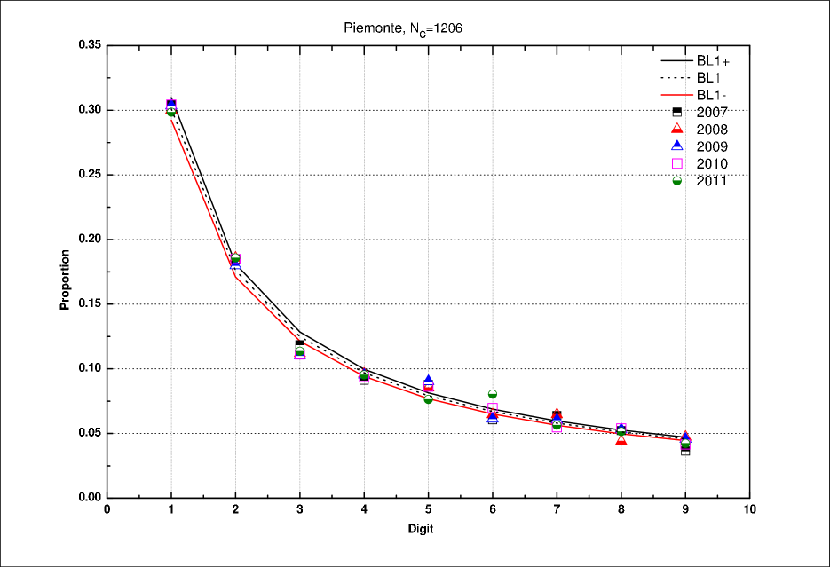
Figure 1: Lombardia.

Figure 2: Piemonte.

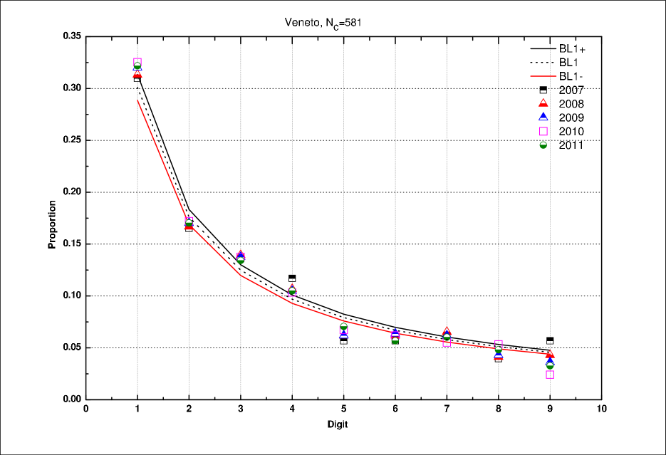
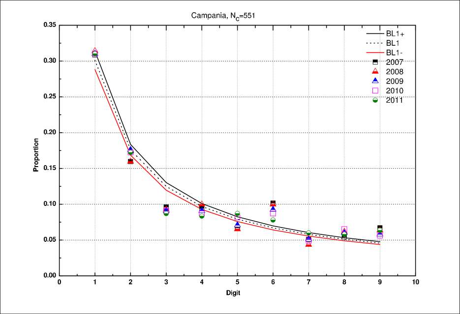
Figure 3: Veneto..

Figure 4: Campania.

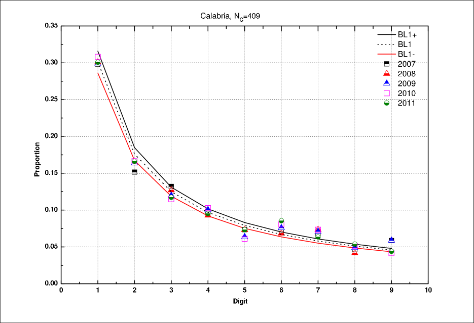
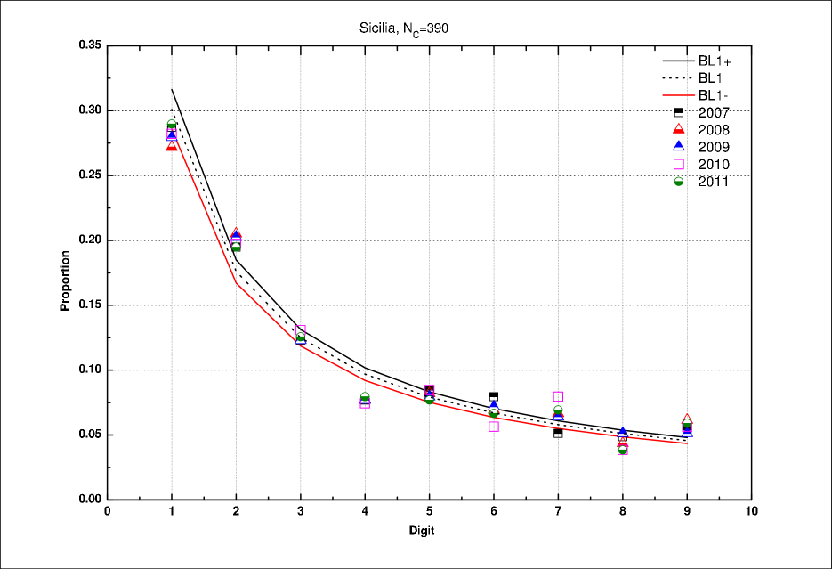
Figure 5: Calabria.

Figure 6: Sicilia.

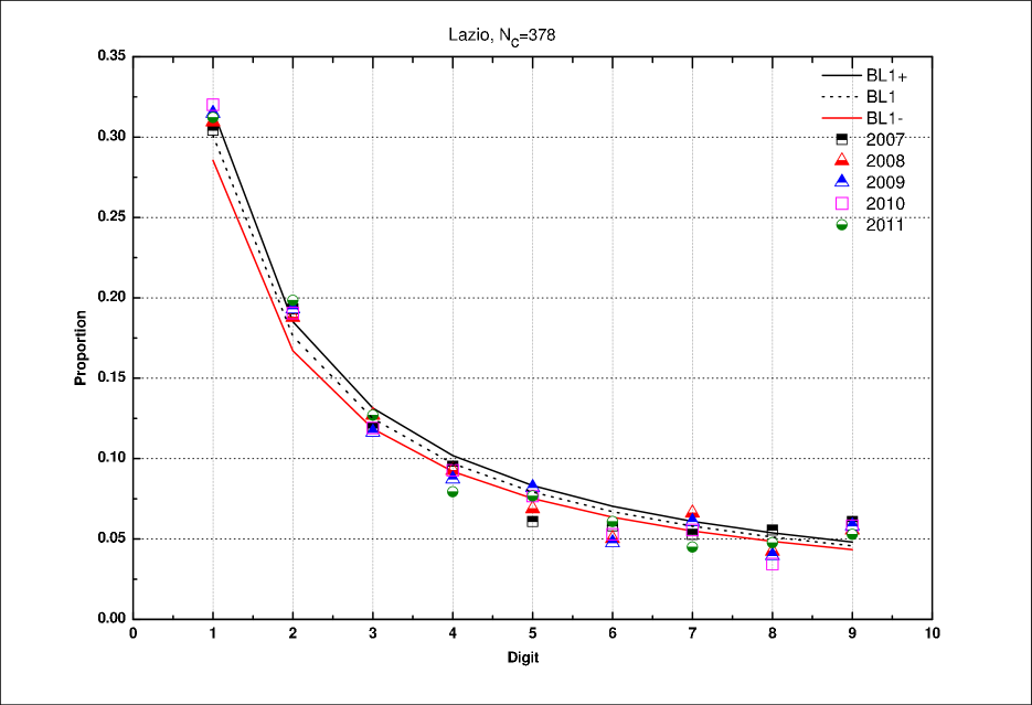
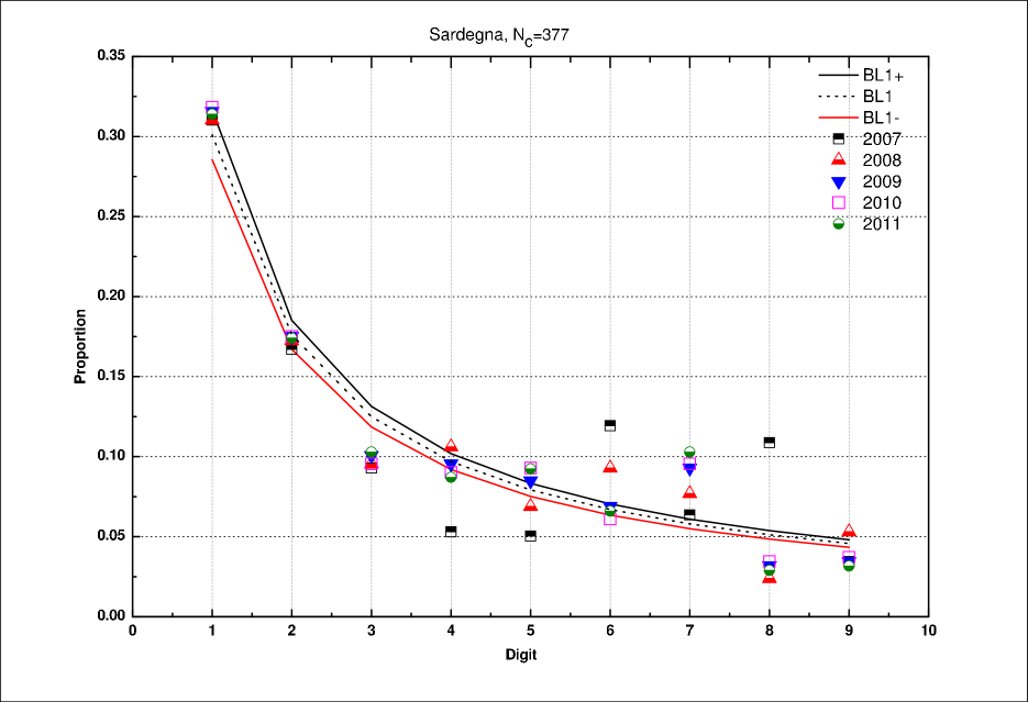
Figure 7: Lazio.

Figure 8: Sardegna.

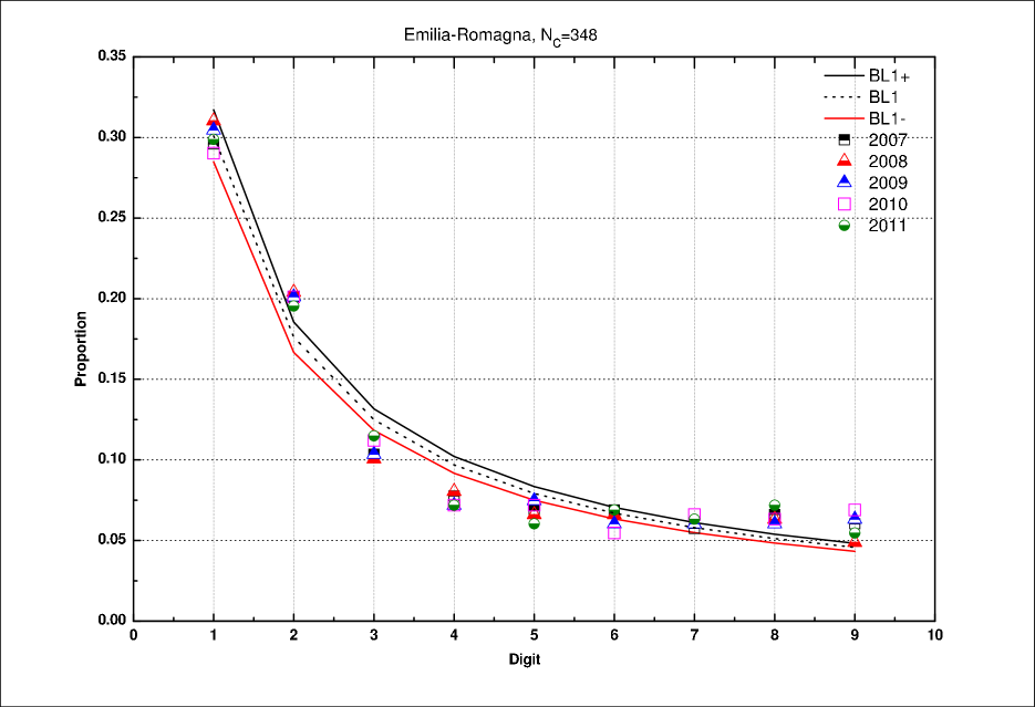
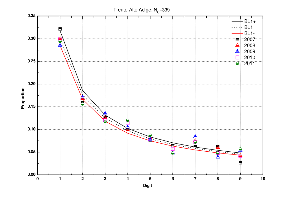
Figure 9: Emilia-Romagna.

Figure 10: Trento-Alto Adige.

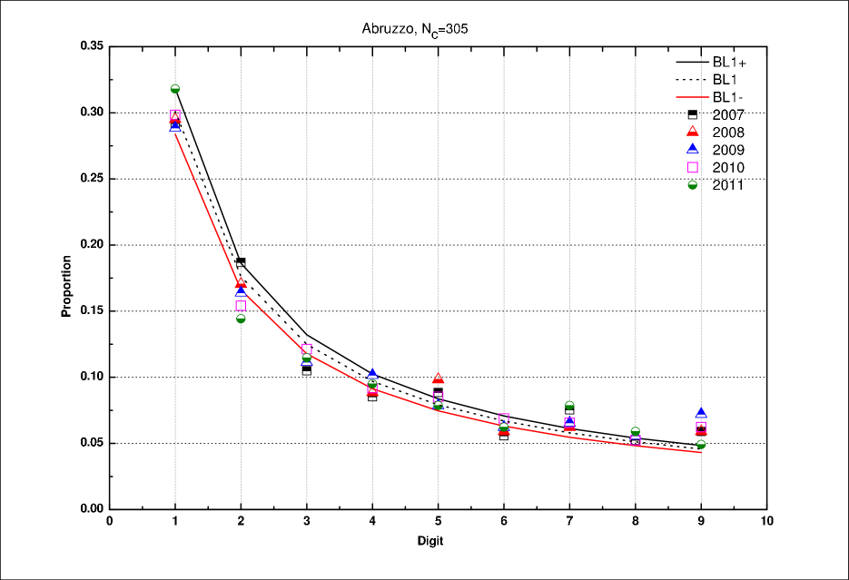
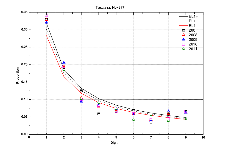
Figure 11: Abruzzo.

Figure 12: Toscana.

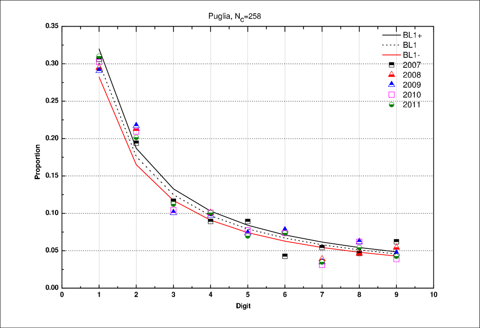
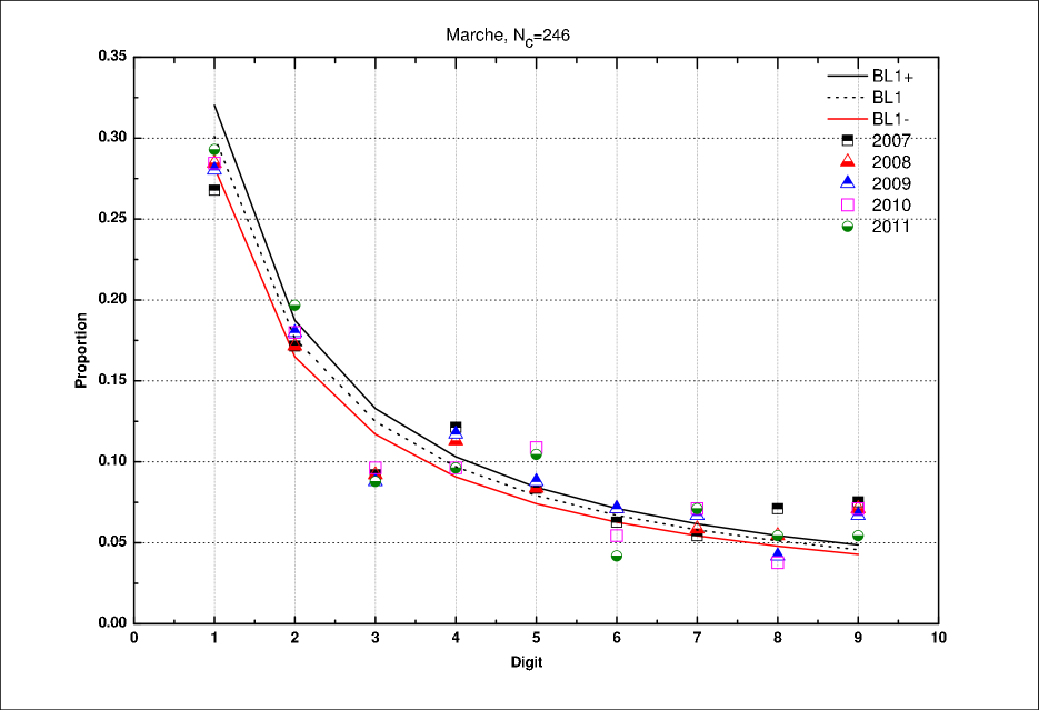
Figure 13: Puglia.

Figure 14: Marche.

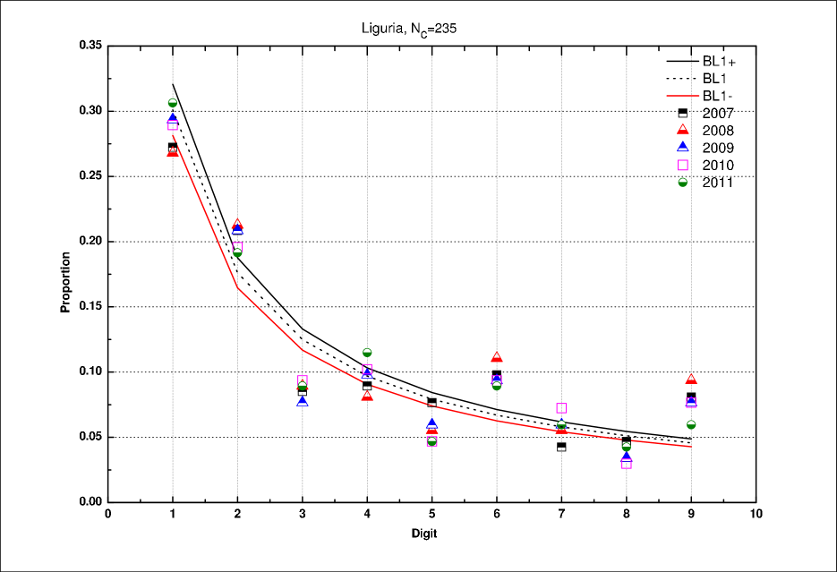
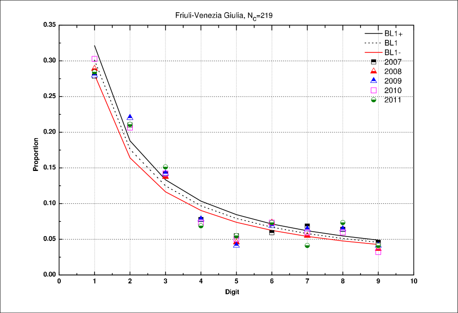
Figure 15: Liguria.

Figure 16: Friuli-Venezia Giulia.

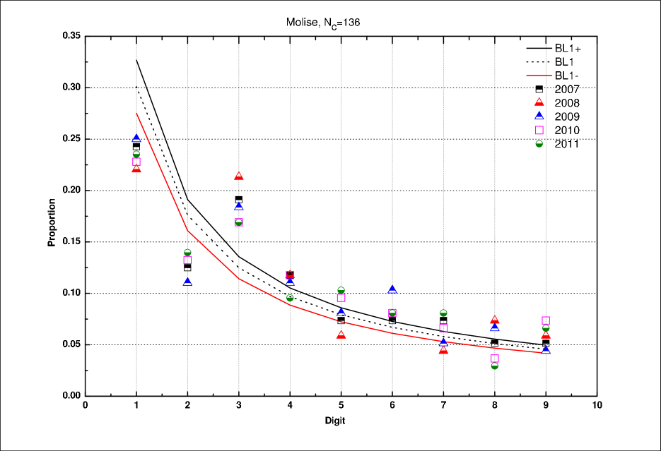
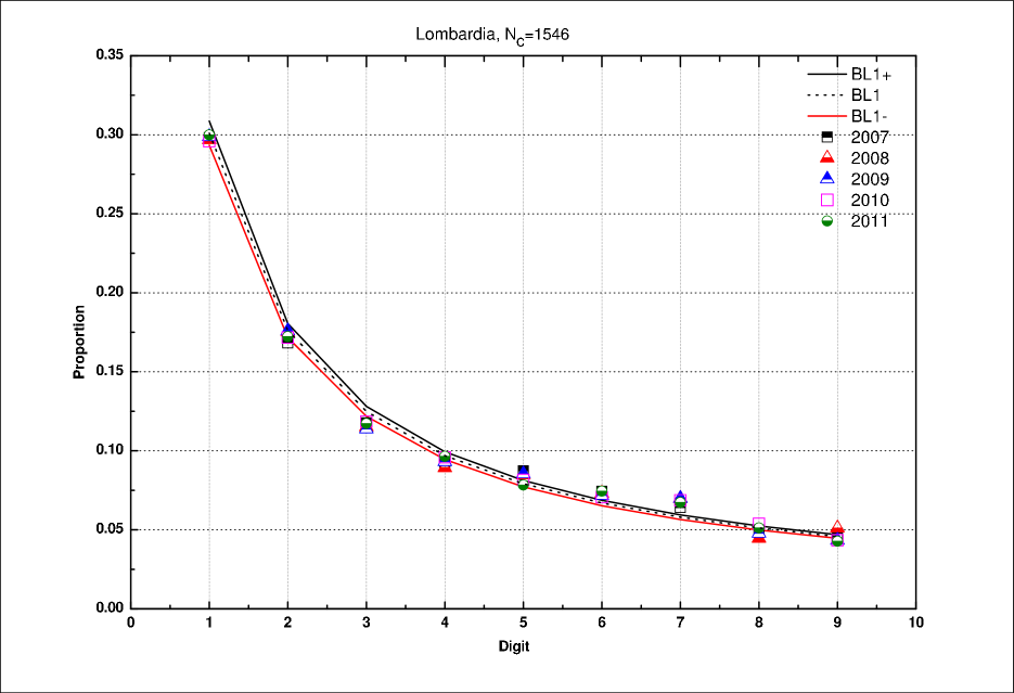
Figure 17: Molise.

Figure 18: Basilicata.

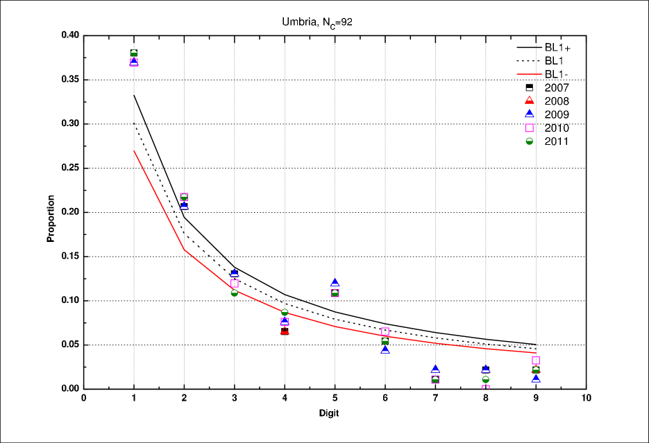
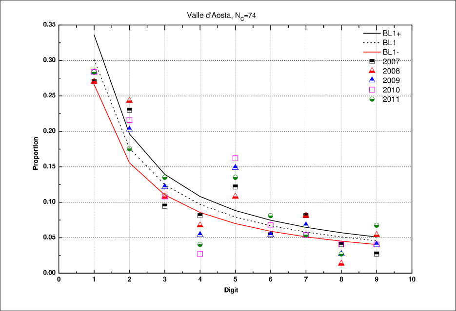
Figure 19: Umbria.

Figure 20: Valle d’Aosta.

Each BL1 data set for each (20) region is displayed on Figs. 1-20; different symbols are used in order to distinguish the 5 years so examined. On each figure, the frequency of the $d$ digit is given, together with the theoretical BL1. Moreover, the sample standard error bar, i.e. depending on the number of cities, i.e. $\sigma\simeq(1/\sqrt{(N_{c,r}-1)})$ allows to draw the estimated range of the confidence interval defined as [BL1-, BL1+], in obvious notations. The display order has been chosen according to the region ranking given in Table 2.

Denote the first digit as $d$, so that $d=1,\dots,9$. Visual observations (list in descending order of $N_{c,r}$) point to:

• Lombardia: rather smooth distribution, not too far from confidence interval (CI); $d=6,7$ somewhat away from CI; above BL1+.

• Piemonte: rather smooth distribution, not too far from CI; $d=5,6$ somewhat away from CI, specifically above BL1+.

• Veneto: rather smooth distribution, not too far from CI, even if $d=4,5$ are somewhat away from CI, on different sides of BL1. $d=9$ is much dispersed.

• Campania: very scattered, except $d=1,2$; other digits are far from CI.

• Calabria: rather smooth distribution, not too far from CI; $d=6,7$ somewhat away from CI, above BL1+; the digit $d=2$ is below BL1-.

• Sicilia: $d=1,4$ below BL1-; $d=7$ much dispersed.

• Lazio: rather smooth distribution, not too far from CI, even if $d=4,5,6$ are somewhat away from CI (below BL1-).

• Sardegna: very very scattered, except for $d=1,2$.

• Emilia-Romagna: rather smooth distribution, not too far from CI. $d=3,4,5$ are somewhat away from CI and below BL1-. The digit $d=8$ is quite above BL1+.

• Trentino-Alto Adige: rather smooth distribution, not too far from CI, but $d=4$ somewhat away from CI (above BL1+). $d=7$ is quite above BL1+, while $d=6$ somewhat below BL1-.

• Abruzzo: rather smooth distribution, but scattered away from CI; on different sides of BL1.

• Toscana: much dispersed; $d=3,4,6,7$ below BL1-; $d=8,9$ quite above BL1+.

• Puglia: much dispersed; $d=3,6,7$ much below BL1-; the digits $d=2,9$ are quite above BL1+.

• Marche: very much dispersed; the digits $d=3,6$ are much below BL1-, while $d=4,5,8,9$ are quite above BL1+.

• Liguria: very much dispersed. The digits $d=3,6,8$ are much below BL1-, while $d=2,4,6,9$ are quite above BL1+.

• Friuli-Venezia Giulia : rather smooth distribution, but rather far from CI; $d=4,5,7$ quite away from CI , below BL1-; $d=2,3,8$ rather away above BL1+.

• Molise: very much scattered from BL1. The digits $d=1,2$ are much much below BL1-, while $d=3,6$ are much much above BL1+. Wide variation for other digits.

• Basilicata: much scattered from BL1. The digits $d=4,8$ are much below BL1-, while $d=5,6$ are much above BL1+. A wide variation for all digits is observed.

• Umbria: much scattered from BL1. The digits $d=4,6,7,8,9$ are much below BL1-, while $d=1,2,5$ are much above BL1+. Also in this case, wide variation for all digits

• Valle d’Aosta: much scattered from BL1. $d=4,8$ are much below BL1-, and $d=2,5,7$ are much above BL1+. Once again, there is wide variation for all digits

4.2 $\chi^{2}$ conformity test

It has been emphasized that there are five $\chi^{2}$ values to be calculated for each region, - one for each year. These 1one hundred $\chi^{2}$ values are found in Tables 5-7. Moreover, the resulting $\chi^{2}$ for the time average values of the AIT is also given,- but recalled that it is given in Table 2 for simplifying the reading of the Tables 5-7.

However, before examining each region BL1, it seems fair to examine whether the distribution of the $\chi^{2}$ itself is anomalous, - in order to pin point (if it occurs) some statistical anomaly arising from computations. Such a distribution of the 100 (20 regions, 5 years) $\chi^{2}$ is shown in Fig. 21.

The distribution is markedly positively skewed, but rather irregular, with a set of outliers. Recall that the critical value of the $\chi^{2}$ at a significance level $0.05$ is $\chi^{2}_{0.05}=15.51$ when the number of degrees of freedom is $\partial=8$ - that of BL1. This rather highly peaked distribution with a few outliers (in particular Sardegna and Liguria, - noticed in different fiscal years) is another hint toward pursuing a BL1 analysis at the regional basis.

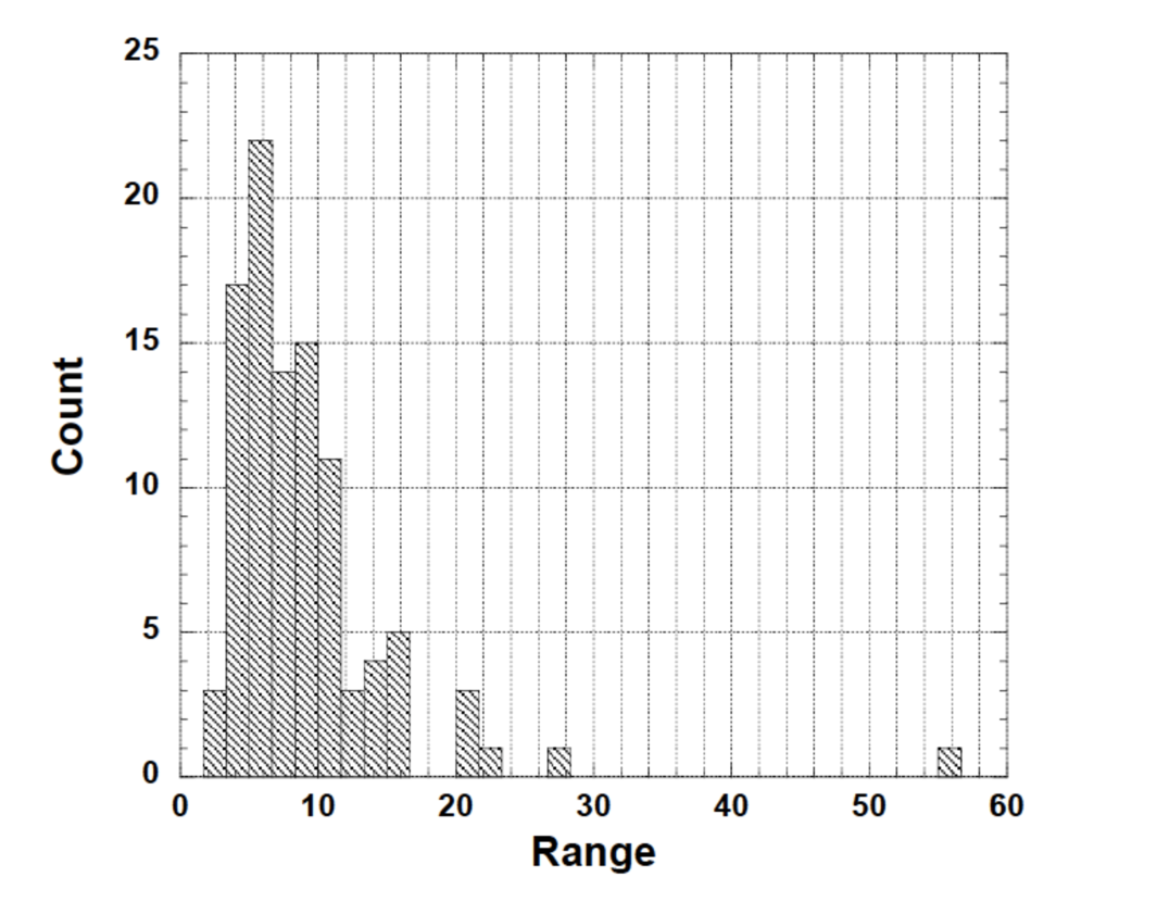
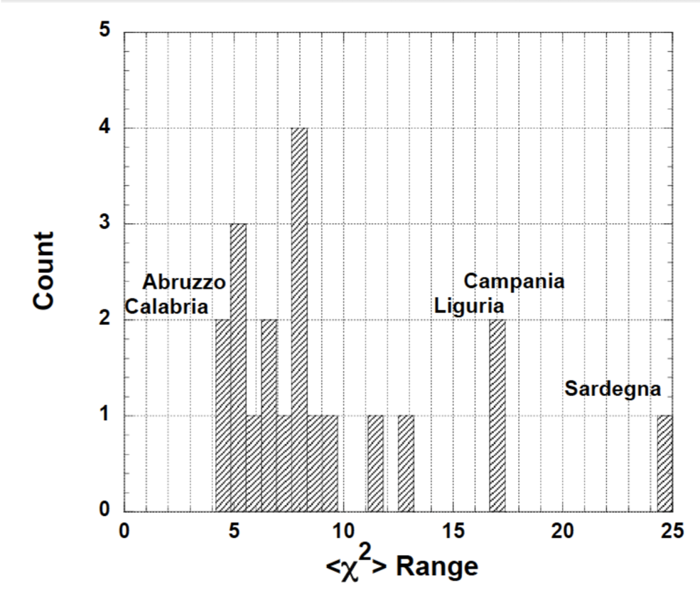
Figure 21: Distribution of yearly $\chi^{2}$ values in BL1 analysis of AIT in the 20 IT regions.

Figure 22: Distribution of the mean (average over the quinquennium) $\chi^{2}$ values in BL1 analysis of AIT in the 20 IT regions.

For emphasizing the regional aspects, and connecting with Table 2 last column, the distribution of the $mean$ (average over the quinquennium) $<\chi^{2}>$ for each region, is shown in Fig. 22. Three regions are markedly outliers in the upper range: Sardegna, Campania and Liguria, for approximately $<\chi^{2}>\geq 15$, pointing to much (questionable) non-conformity with BL1. On the contrary, 2 regions have a low $<\chi^{2}>$ over the quinquennium, Abruzzo and Calabria, indicating very fine agreement with BL1 ($<\chi^{2}>\leq 4$).

At this stage, it seems important to point to a quite substantial time-invariance of the $\chi^{2}$ values, according to the displayed data/.

Thereafter, it seems natural to discuss each region BL1 values, to notice conformity or not, starting from the most valid and ending with the most anomalous. In so doing, one can distinguish values according to the standard risk value for rejecting the null hypothesis, i.e. a uniform distribution, at $\chi^{2}_{0.05}=15.507$ for a number of degrees of freedom $\partial=8$; for completeness, let us observe that (for $\partial=8$) the critical value of the $\chi^{2}$ at a significance level $0.10$ is $\chi^{2}_{0.10}=13.362$.

4.2.1 $<\chi^{2}>\leq 13.362$, and yearly (ir)regularity

It is found from Table 2 that the BL1 $<\chi^{2}>$ has a small value in 17 regions; from the lowest to the highest: Calabria (4.4664), Abruzzo (4.7372), Lazio (5.0288), Piemonte (5.2830) Trentino-Alto Adige (5.3782), Puglia (5.8868) Lombardia (6.3694) Sicilia (6.4494) Basilicata (7.5054), Valle d’Aosta (7.6682), Veneto (7.7896), Friuli-Venezia Giulia (7.8444), Emilia-Romagna (8.1620), Marche (8.6922), Toscana (9.5140), Umbria (11.317) and Molise (12.657).

Among these, Tables 5-7 show that much regularity is observed in the respective yearly values, with some exceptions.

The values for Veneto (11.33) in 2007, Emilia-Romagna (10.60) in 2010, and Valle d’Aosta (11.31) in 2010 are such that the respective $\chi^{2}$ fall outside the 5% sampling error bar. The largest $\chi^{2}$ value for Molise occurs in 2008, $\sim$ 20.99, although a surprisingly quite small $\chi^{2}$ value $\sim$ 9.74 occurs in 2007. The $\chi^{2}$ values for Umbria are high, but without any severe hint of an anomaly; the distribution of $\chi^{2}$ values is quite narrow indeed for Umbria, implying some systematicity.

4.2.2 $<\chi^{2}>\geq 15.507$, and yearly (ir)regularity

In contrast, Liguria (16.895), Campania (17.224), and Sardegna (24.587) are the 3 regions with an indication of much lack of conformity with respect to BL1.

The two largest $\chi^{2}$ values for Sardegna occur in 2007 and 2011: $\sim$ 56.00 and 21.36, respectively. The largest $\chi^{2}$ values for Campania occur in 2007 and 2008: $\sim$ 21.65 and 23.02, respectively. The largest $\chi^{2}$ value for Liguria occurs in 2008: $\sim$ 27.17; surprisingly, a quite small $\chi^{2}$ value $\sim$ 9.70 occurs in 2011.

5 Discussion

This section fixes and discusses the results of the investigation.

In general, the concordance between the AIT of Italian regions and the theoretical statement of BL1 is rather questionable. There are discrepancies at a regional level, an this is in line with the heterogeneous nature of Italian regions under a socio-economic point of view. In particular, one can note a very good matching between geographic and economic features of the regions, and cluster them among $N$ (North), $C$ (Center), $S$ (South, plus Sicilia and Sardegna).

$N$ is the part of Italy constituted by 8 regions: Emilia-Romagna, Friuli-Venezia Giulia, Liguria, Lombardia, Piemonte, Trentino-Alto Adige, Valle d’Aosta and Veneto;

$C$ contains 5 regions: Abruzzo, Lazio, Marche, Toscana and Umbria;

$S$ is the remaining 7 regions: Basilicata, Calabria, Campania, Molise, Puglia, Sardegna, Sicilia.

Deviations from BL1 are usually read as ”data manipulation”. However, the law is surely a subject of controversy in accounting. It is not clear even now neither why it should be valid at all, under whatever ”socio-economic conditions”, nor whether its theoretical derivation, under various hypotheses, informs us on its origins and its range of applications. Even Newcomb and Benford were dubious of the realm of validity. Therefore, a deep exploration of the regional reality behind the AIT data, of how they have been collected and of the shadow economy at a regional level are required to provide a rigorous interpretation of the results. This is well-beyond the scopes of this paper. We can only give some suggestions and discussions, to be likely taken as arguments for future studies.

Among the 3 regions with very anomalous BL1 $\chi^{2}$, two belong to $S$: Sardegna and Campania, while the other comes from $N$: Liguria.

Sardegna is characterized by a noticeable fragmentation at a city level in several municipalities with very small number of inhabitants. This region does not have a highly developed industrial structure, and a wide part of the regional economy is still based on agriculture and livestock. In the small communities the economy is somewhat closed, and business exchanges are often based on commodities. In such a situation, one can guess that the existence of a discrepancy between the official data and the income tax should come from the real regional economy.

Sadly, Campania has the relevant problem of a massive influence of the organized crime on the economic system. Hence, deviations from BL1 can be viewed ”as expected”.

The economic system of Liguria seems to be affected by the pervasion of shadow economy. Confartigianato (the Italian association of artisans and small businesses) states that about 73% of the artisans is in competition with illegal and shadow economies (see $http://www.confartigianatoliguria.it/node/4153$). This evidence represents a good hint for explaining why Liguria exhibits this discrepancy with respect to BL1.

Unexpectedly, we admit so, the remaining regions are in accordance with the BL1, with some disparities over the quinquennium as highlighted in the previous Section. From both an economic and a social point of view, some regions are quite similar to Campania, with a remarkable presence of organized crime (think at Calabria, Puglia and Sicilia, but also to the North with Veneto and Lombardia). Basilicata and Molise are similar to Sardegna for what concerns the absence of a well-established industrial structure. It is also worth mentioning that Basilicata is the main producer of fossil fuels in Italy (see the report in $http://www.siteb.it/new\%20siteb/documenti/RASSEGNA/6711_{7}.pdf$). Moreover, shadow economy is generally widespread in the entire country.

To conclude: we demonstrate some hints for further exploring cases of violations of BL1, whence likely possible tax income manipulation through accounting city Aggregated Income Tax reports throughout all Italian Regions. We admit that not every finding can be explained only based on BL1: we do not understand why some regions do not have BL1 violators; we avoid to propose speculative statements which might be called ”resulting from imagination”. Yet, this further supports the point that a deeper analysis should be carried out to investigate the nature of the fiscal data and how they are usually collected and approved (Pentland and Carlile 1996).

6 Conclusions

Today Benford’s law is routinely used by forensic analysts to detect error, incompleteness and dubious manipulation of financial data. The basic premise of the test is that the first digits in real data, in general, have a tendency to approach the Benford distribution whereas people intending to play with the numbers, when unaware of the law, try to place the digits uniformly. Thus any departure from the law raises some suspicion. We have assessed the tax income possible manipulation of citizens in Italy through accounting city aggregated income tax reports from all Italian regions, with data obtained from the Research Center of the Italian MEF.

The validity of the reported data does not seem to have attracted official accountants. For example, something like Economia e Finanza locale Rapporto 2010 or RAPPORTO ANNUALE 2012 La situazione del Paese fall short of discussing the data validity.

This paper provides an examination of a fiscal data set stemming from the Italian citizens, on a regional level. Specifically, it focuses on the assessment of potential manipulation of tax income through the adoption of the Benford law for the first digit over the quinquennium 2007-2011.

The BL1 presents significant advantages over alternative measures of accounting quality currently used in practice. For example, it does not require time-series, cross-sectional, or forward-looking information, nor details on ”transactions”.

Throughout the paper we refer to municipalities, though in practice we are investigating the incomes of citizens, but we avoid any individual information on whether individuals correctly report their income. This is an important distinction to the extent that this is precisely the population set of interest. Though we find significant variations in municipality tax incomes by regions, much of the variation is actually attributable to differences in the characteristics of regions

Another purpose of this paper has been to provide a proof of the BL1 concept for using the fiscal data at a regional level in order to provide some information on manipulation. It is shown that it is possible to document the variation in income taxes across regions, to order them, and to observe a distribution of anomalies, also in time. The sampling data at this aggregated level is large enough to look in details at pertinent numbers, - without making strong econometric modeling assumptions. The restriction on the demand of a large database (at the country level) expected to provide the scale needed for the data to be sufficiently granular can be relaxed. The data analysis points to different regional realities, sometimes quite unexpectedly.

Durtschi et.al (2004) have pointed out that when interpreting results of Benford’s law, one should be aware of a few risks: However, Benford law is most effective for large data set, when data represents more than one distribution, when the mean is greater than the median, and the skewness is positive. This seems to be the case in our investigation.

Our findings demonstrate also that Benford’s law seems effective in detecting data bias in not too large data sets. There is (alas) no doubt that manipulation of income reports exist in various regions and municipalities. Either a few accountants are so well aware that BL1 is a test and can avoid the non-conformity surprise, at the individual level, but cannot do so at the next (city aggregation) level.

Thus, to our knowledge, this paper is the first to document whether income tax aggregated data conforms to the (first) Benford’s law, i.e. how without examining (individual) citizens financial reports are likely to exhibit divergences. In so doing, a view of fraud or manipulation is put on a more collective level.

Acknowledgements

This paper is part of scientific activities in COST Action IS1104, ”The EU in the new complex geography of economic systems: models, tools and policy evaluation”.

Appendix: figures and big tables

Digit	1	2	3	4	5	6	7	8	9	$\chi^{2}$
Year	Lombardia, $N_{c}=$ 1546 for 2007-2019 ; $N_{c}=$ 1544 for 2010-2011
2007	0.298	0.168	0.118	0.092	0.087	0.074	0.064	0.050	0.048	5.297
2008	0.297	0.175	0.115	0.089	0.085	0.073	0.070	0.045	0.051	9.692
2009	0.299	0.176	0.114	0.093	0.085	0.072	0.070	0.048	0.043	7.348
2010	0.296	0.172	0.119	0.096	0.082	0.071	0.069	0.054	0.043	4.674
2011	0.300	0.172	0.117	0.097	0.078	0.074	0.067	0.051	0.043	4.836
	Piemonte, $N_{c}=$ 1206
2007	0.304	0.185	0.119	0.091	0.088	0.061	0.064	0.052	0.036	6.279
2008	0.300	0.186	0.112	0.096	0.085	0.065	0.065	0.044	0.047	5.175
2009	0.303	0.180	0.110	0.095	0.090	0.061	0.061	0.053	0.046	4.925
2010	0.304	0.185	0.111	0.094	0.086	0.070	0.055	0.054	0.041	4.327
2011	0.299	0.186	0.114	0.095	0.076	0.080	0.056	0.051	0.042	5.709
	Veneto, $N_{c}=$ 581
2007	0.310	0.165	0.136	0.117	0.057	0.057	0.062	0.040	0.057	11.327
2008	0.313	0.167	0.139	0.107	0.062	0.062	0.065	0.041	0.043	6.251
2009	0.320	0.170	0.138	0.105	0.062	0.064	0.062	0.043	0.036	6.309
2010	0.325	0.172	0.138	0.103	0.067	0.062	0.055	0.053	0.024	9.569
2011	0.322	0.170	0.134	0.105	0.071	0.057	0.060	0.048	0.033	5.492
	Campania, $N_{c}=$ 551
2007	0.309	0.160	0.096	0.094	0.067	0.102	0.051	0.054	0.067	21.647
2008	0.314	0.160	0.093	0.100	0.065	0.100	0.044	0.062	0.064	23.021
2009	0.310	0.176	0.091	0.091	0.071	0.093	0.051	0.060	0.058	14.559
2010	0.310	0.172	0.091	0.087	0.082	0.087	0.049	0.065	0.056	13.556
2011	0.310	0.172	0.087	0.083	0.087	0.078	0.060	0.058	0.064	13.336
	Calabria, $N_{c}=$ 409
2007	0.298	0.152	0.132	0.098	0.073	0.073	0.068	0.046	0.059	4.439
2008	0.301	0.164	0.127	0.093	0.073	0.068	0.073	0.042	0.059	4.514
2009	0.298	0.164	0.120	0.100	0.064	0.076	0.071	0.049	0.059	4.939
2010	0.308	0.166	0.115	0.103	0.061	0.081	0.073	0.051	0.042	5.420
2011	0.301	0.166	0.117	0.095	0.073	0.086	0.064	0.054	0.044	3.020
	Sicilia, $N_{c}=$ 390
2007	0.287	0.195	0.123	0.077	0.085	0.079	0.051	0.049	0.054	4.614
2008	0.272	0.205	0.123	0.077	0.082	0.069	0.067	0.044	0.062	7.728
2009	0.279	0.203	0.123	0.077	0.079	0.072	0.064	0.051	0.051	4.421
2010	0.282	0.197	0.131	0.074	0.085	0.056	0.079	0.038	0.056	9.723
2011	0.290	0.195	0.126	0.079	0.077	0.067	0.069	0.038	0.059	5.761
	Lazio, $N_{c}=$ 378
2007	0.304	0.193	0.119	0.095	0.061	0.058	0.053	0.056	0.061	4.980
2008	0.310	0.188	0.127	0.093	0.069	0.050	0.066	0.042	0.056	4.360
2009	0.315	0.193	0.116	0.087	0.082	0.048	0.061	0.040	0.058	5.894
2010	0.320	0.190	0.119	0.093	0.077	0.053	0.056	0.034	0.058	5.613
2011	0.312	0.198	0.127	0.079	0.077	0.061	0.045	0.048	0.053	4.297

Table 5: Frequencies of the first digit in reported AIT data for IT regions with a high $N_{c}$ number, for various years; it can be visually compared to the expected frequency according to BL given in Table 1; the corresponding calculated $\chi^{2}$ is to be compared with the theoretical one (15.507) for a number of degree of freedom ($\partial=8$) at $0.05\%$. The null hypothesis is not verified for underlined cases.

Digit	1	2	3	4	5	6	7	8	9	$\chi^{2}$
Year	Sardegna, $N_{c}=$ 337
2007	0.310	0.167	0.093	0.053	0.050	0.119	0.064	0.109	0.034	56.001
2008	0.310	0.172	0.095	0.106	0.069	0.093	0.077	0.024	0.053	15.606
2009	0.316	0.175	0.101	0.095	0.085	0.069	0.093	0.032	0.034	13.908
2010	0.318	0.175	0.095	0.090	0.093	0.061	0.095	0.034	0.037	16.059
2011	0.314	0.174	0.103	0.087	0.092	0.066	0.103	0.029	0.032	21.363
	Emilia-Romagna, $N_{c}=$ 348
2007	0.296	0.201	0.103	0.078	0.069	0.069	0.057	0.066	0.060	7.516
2008	0.310	0.204	0.101	0.080	0.066	0.066	0.060	0.063	0.049	6.121
2009	0.305	0.201	0.103	0.072	0.075	0.060	0.060	0.060	0.063	8.040
2010	0.290	0.201	0.112	0.072	0.072	0.055	0.066	0.063	0.069	10.604
2011	0.299	0.195	0.115	0.072	0.060	0.069	0.063	0.072	0.055	8.529
	Trentino-Alto Adige, $N_{c}=$ 339
2007	0.322	0.159	0.127	0.100	0.077	0.065	0.062	0.062	0.027	4.713
2008	0.300	0.168	0.126	0.099	0.081	0.048	0.075	0.060	0.042	4.225
2009	0.285	0.171	0.135	0.105	0.078	0.048	0.084	0.039	0.054	7.975
2010	0.300	0.168	0.120	0.114	0.078	0.057	0.072	0.048	0.042	2.992
2011	0.294	0.156	0.117	0.120	0.087	0.048	0.072	0.048	0.057	6.986
	Abruzzo, $N_{c}=$ 305
2007	0.292	0.187	0.105	0.085	0.089	0.056	0.075	0.052	0.059	5.381
2008	0.295	0.170	0.111	0.089	0.098	0.059	0.062	0.056	0.059	3.852
2009	0.289	0.164	0.111	0.102	0.079	0.062	0.066	0.056	0.072	6.090
2010	0.298	0.154	0.121	0.092	0.085	0.069	0.066	0.052	0.062	3.252
2011	0.318	0.144	0.115	0.095	0.079	0.062	0.079	0.059	0.049	5.111
	Toscana, $N_{c}=$ 287
2007	0.331	0.188	0.125	0.059	0.066	0.070	0.035	0.059	0.066	11.580
2008	0.328	0.195	0.105	0.080	0.070	0.059	0.042	0.059	0.063	7.097
2009	0.321	0.206	0.094	0.084	0.073	0.056	0.038	0.066	0.063	10.148
2010	0.341	0.195	0.101	0.084	0.066	0.059	0.042	0.045	0.066	8.958
2011	0.369	0.185	0.101	0.091	0.073	0.042	0.056	0.038	0.045	9.787
	Puglia, $N_{c}=$ 258
2007	0.306	0.194	0.116	0.089	0.089	0.043	0.054	0.047	0.062	5.060
2008	0.295	0.213	0.101	0.101	0.074	0.078	0.039	0.047	0.054	5.989
2009	0.291	0.217	0.101	0.097	0.074	0.078	0.035	0.062	0.047	7.260
2010	0.302	0.209	0.105	0.101	0.078	0.074	0.031	0.062	0.039	6.800
2011	0.310	0.202	0.112	0.101	0.070	0.074	0.035	0.054	0.043	4.325

Table 6: Frequencies of the first digit in reported AIT data for IT regions with a medium range $N_{c}$ number, for various years; it can be visually compared to the expected frequency according to BL given in Table 1; the corresponding calculated $\chi^{2}$ is to be compared with the theoretical one (15.507) for a number of degree of freedom ($\partial=8$) at $0.05\%$. The null hypothesis is always verified in these cases.

Digit	1	2	3	4	5	6	7	8	9	$\chi^{2}$
Year	Marche, $N_{c}=$ 239
2007	0.268	0.172	0.092	0.121	0.084	0.063	0.054	0.071	0.075	11.051
2008	0.285	0.172	0.092	0.113	0.084	0.071	0.059	0.054	0.071	6.486
2009	0.280	0.180	0.088	0.117	0.088	0.071	0.067	0.042	0.067	7.370
2010	0.285	0.180	0.096	0.096	0.109	0.054	0.071	0.038	0.071	9.946
2011	0.293	0.197	0.088	0.096	0.105	0.042	0.071	0.054	0.054	8.608
	Liguria, $N_{c}=$ 235
2007	0.272	0.209	0.085	0.089	0.077	0.098	0.043	0.047	0.081	15.920
2008	0.268	0.213	0.089	0.081	0.055	0.111	0.055	0.034	0.094	27.173
2009	0.294	0.209	0.077	0.098	0.060	0.094	0.060	0.034	0.077	15.719
2010	0.289	0.196	0.094	0.102	0.047	0.094	0.072	0.030	0.077	15.954
2011	0.306	0.191	0.089	0.115	0.047	0.089	0.060	0.043	0.060	9.707
	Friuli-Venezia Giulia, $N_{c}=$ 219 for 2007 ; $N_{c}=$ 218 for 2008-2011
2007	0.279	0.210	0.142	0.078	0.055	0.059	0.068	0.064	0.046	6.075
2008	0.289	0.220	0.138	0.078	0.046	0.073	0.055	0.064	0.037	7.940
2009	0.280	0.220	0.142	0.078	0.041	0.069	0.064	0.064	0.041	8.993
2010	0.303	0.206	0.142	0.073	0.050	0.073	0.060	0.060	0.032	6.516
2011	0.284	0.211	0.151	0.069	0.055	0.073	0.041	0.073	0.041	9.698
	Molise, $N_{c}=$ 136
2007	0.243	0.125	0.191	0.118	0.074	0.074	0.074	0.051	0.051	9.741
2008	0.221	0.110	0.213	0.118	0.059	0.103	0.044	0.074	0.059	20.990
2009	0.250	0.110	0.184	0.110	0.081	0.103	0.051	0.066	0.044	11.890
2010	0.228	0.132	0.169	0.118	0.096	0.081	0.066	0.037	0.074	10.475
2011	0.235	0.140	0.169	0.096	0.103	0.081	0.081	0.029	0.066	10.190
	Basilicata, $N_{c}=$ 131
2007	0.290	0.160	0.130	0.061	0.122	0.076	0.061	0.023	0.076	9.965
2008	0.282	0.168	0.107	0.107	0.084	0.092	0.031	0.061	0.069	5.365
2009	0.290	0.160	0.122	0.099	0.061	0.099	0.053	0.053	0.061	3.567
2010	0.290	0.168	0.115	0.092	0.076	0.122	0.023	0.053	0.061	9.692
2011	0.305	0.160	0.099	0.115	0.053	0.122	0.046	0.046	0.053	8.938
	Umbria, $N_{c}=$ 92
2007	0.380	0.207	0.130	0.065	0.109	0.054	0.011	0.022	0.022	10.855
2008	0.370	0.207	0.130	0.065	0.120	0.043	0.022	0.022	0.022	10.348
2009	0.370	0.207	0.130	0.076	0.120	0.043	0.022	0.022	0.011	11.093
2010	0.370	0.217	0.120	0.076	0.109	0.065	0.011	0.000	0.033	12.352
2011	0.380	0.217	0.109	0.087	0.109	0.054	0.011	0.011	0.022	11.938
	Valle d’Aosta, $N_{c}=$ 74
2007	0.270	0.230	0.095	0.081	0.122	0.054	0.081	0.041	0.027	5.456
2008	0.270	0.243	0.108	0.068	0.108	0.054	0.081	0.014	0.054	6.760
2009	0.284	0.203	0.122	0.054	0.149	0.054	0.068	0.027	0.041	7.477
2010	0.284	0.216	0.108	0.027	0.162	0.068	0.054	0.041	0.041	11.309
2011	0.284	0.176	0.135	0.041	0.135	0.081	0.054	0.027	0.068	7.339

Table 7: Frequencies of the first digit in reported AIT data for IT regions with a low $N_{c}$ number, for various years; it can be visually compared to the expected frequency according to BL given in Table 1; the corresponding calculated $\chi^{2}$ is to be compared with the theoretical one (15.507) for a number of degree of freedom ($\partial=8$) at $0.05\%$. The null hypothesis is not verified for underlined cases.

References

- [1] Abrantes-Metz, R.M., Villas-Boas, S.B., Judge, G., (2011). Tracking the Libor rate. Applied Economics Letters, 18(10), 893-899.
- [2] Aggarwal, R., & Lucey, B.M., (2007). Psychological barriers in gold prices?. Review of Financial Economics, 16(2), 217-230.
- [3] Alali F.A , & Romero S., (2013). Benford’s Law: Analyzing a decade of financial data. Journal of Emerging Technologies in Accounting, 10(1), 1-39.
- [4] Alexeev, M., Janeba, E., & Osborne, S., (2004). Taxation and evasion in the presence of extortion by organized crime. Journal of Comparative Economics, 32, 375-387.
- [5] Amiram, D., Bozanic, Z., & Rouen, E., (2015). Financial statement errors: evidence from the distributional properties of financial statement numbers. Review of Accounting Studies, 20(4), 1540-1593; ibid. Erratum to: Financial statement errors: evidence from the distributional properties of financial statement numbers. Review of Accounting Studies, 20(4), 1594-1595.
- [6] Armstrong, C.S., Blouin, J.L., Jagolinzer, A.D., & Larcker, D.F. (2015). Corporate governance, incentives, and tax avoidance. Journal of Accounting and Economics, 60(1), 1-17.
- [7] Ausloos, M., Herteliu, C., & Ileanu, B., (2015). Breakdown of Benford’s law for birth data. Physica A, 419, 736-745.
- [8] Ausloos, M., Castellano, R., & Cerqueti, R., (2016). Regularities and Discrepancies of Credit Default Swaps: a Data Science approach through Benford’s Law. Chaos, Solitons and Fractals, doi:10.1016/j.chaos.2016.03.002.
- [9] Bartolini, D., & Santolini, R. (2012). Political yardstick competition among Italian municipalities on spending decisions. The Annals of Regional Science, 49(1), 213-235.
- [10] Beebe, N.H.F., (2016). A Bibliography of Publications about Benford’s Law, Heaps’ Law, and Zipf’s Law.
- [11] Benford, F., (1938). The law of anomalous numbers. Proceedings of the American Philosophical Society, 74 (8), 551-572.
- [12] Bierstaker J.L., Brody, R. G., & Pacini, C., (2006). Accountants’ perceptions regarding fraud detection and prevention methods. Managerial Auditing Journal, 21(5), 520-535
- [13] Bolton, R.J., & Hand, D.J., (2001). Unsupervised profiling methods for fraud detection. Credit Scoring and Credit Control, VII, 235-255.
- [14] Bolton, R.J., & Hand, D.J., (2002). Statistical fraud detection: A review, Statistical Science, 17(3), 235-249.
- [15] Brosio, G., Cassone, A., & Ricciuti, R., (2002). Tax evasion across Italy: rational non- compliance or inadequate civic concern. Public Choice, 112(3), 259-273.
- [16] Calderoni, F., (2011). Where is the mafia in Italy? Measuring the presence of the mafia across Italian provinces. Global Crime, 12(1), 41-69.
- [17] Carbone, A., Jensen, M., Sato, A.H., (2016). Challenges in data science: a complex systems perspective. Chaos, Solitons and Fractals, 90, 1-7.
- [18] Carrera, C., (2015). Tracking exchange rate management in Latin America. Review of Financial Economics, 25, 35-41.
- [19] Ciaponi, F., & Mandanici, F., (2015). Using digital frequencies to detect anomalies in receivables and payables: an analysis of the Italian universities. Ekonomski i socijalni razvoj, 2(1), 86-108.
- [20] Chiarini, B., Marzano, E., & Schneider, F., (2013). Tax rates and tax evasion: an empirical analysis of the long-run aspects in Italy. European Journal of Law and Economics, 35(2), 273-293.
- [21] Cleary, R., & Thibodeau, J. C. (2005). Applying digital analysis using Benford’s law to detect fraud: The dangers of Type I errors. Auditing. A Journal of Practice & Theory, 24(1), 77-81.
- [22] Clippe, P., & Ausloos, M., (2012). Benford’s law and Theil transform of financial data, Physica A, 391(24), 6556-6567.
- [23] Cooper, D.J., Dacin, T., & Palmer, D., (2013). Fraud in accounting, organizations and society: Extending the boundaries of research. Accounting, Organizations and Society, 38(6), 440-457.
- [24] Costa, J. I. F., Santos, J., & Travassos, S.K.M., (2012). An Analysis of Federal Entities Compliance with Public Spending: Applying the Newcomb-Benford Law to the 1st and 2nd Digits of Spending in Two Brazilian States. Revista Contabilidade & Finanças-USP, 23(60), 187-198.
- [25] Costa, J. I. F., Travassos, & S. K. M., Santos, J., (2013). Application of Newcomb-Benford law in accounting audit: a bibliometric analysis in the period from 1988 to 2011. 10th International conference on information systems and technology management, June 12-14 (2013), Sao Paulo, Brazil.
- [26] Davidson, P. (1987). Sensible expectations and the long-run non-neutrality of money. Journal of Post Keynesian Economics, 10(1), 146-153.
- [27] Davidson, P., (1996). Reality and economic theory. Journal of Post Keynesian Economics, 18(4), 479-508.
- [28] Davidson, P., (2009). The Keynes Solution: The Path To Global Economic Prosperity. Palgrave/Macmillan,
- [29] Durtschi, C., Hillison, W., & Pacini, C. (2004). The effective use of Benford’s law to assist in the detecting of fraud in accounting data. Journal of Forensic Accounting, 5, 17-34.
- [30] Fiorio, C.V., & D’Amuri, F., (2005). Workers tax evasion in Italy. Giornale degli Economisti e Annali di Economia, 64 (2/3), 247-270.
- [31] Fu, D., Shi, Y.Q. & Su, W., (2007). A generalized Benford’s law for JPEG coefficients and its applications in image forensics. In: Electronic Imaging, 65051L-65051L International Society for Optics and Photonics.
- [32] Galbiati, R., & Zanella, G. (2012). The tax evasion social multiplier: evidence from Italy. Journal of Public Economics, 96(5), 485-494.
- [33] Gava, A. M, & Vitiello, L., 2014. Inflation, Quarterly Balance Sheets and the Possibility of Fraud: Benford’s Law and the Brazilian case. Journal of Accounting, Business & Management 21, 43-52.
- [34] Guan,L., He, S.D., & Mc Eldowney, J., (2008). Window Dressing in Reported Earnings. Commercial Lending Review, 23 (3), 28-33.
- [35] Haynes A. H. (2012). Detecting Fraud in Bankrupt Municipalities Using Benford’s Law. Scripps Senior Theses., Paper 42. available at .
- [36] Hill, T.P., (1998). The First Digit Phenomenon A century-old observation about an unexpected pattern in many numerical tables applies to the stock market, census statistics and accounting data. American Scientist, 86(4), 358-363.
- [37] Holz, C.A., (2014). The Quality of China’s GDP Statistics. China Economic Review, 30, 309-338.
- [38] Johnson, G.G., & Weggenmann, J., (2013).Exploratory research applying Benford’s law to selected balances in the financial statements of state governments. Academy of Accounting and Financial Studies Journal, 17(1), 31-44.
- [39] Lin, C. C., Chiu, A. A., Huang, S. Y.Y., & Yen, D. C., (2015). Detecting the financial statement fraud: The analysis of the differences between data mining techniques and experts judgments. Knowledge-Based Systems, 89, 459-470.
- [40] Lucas, R.E., & Sargent, T., (1981). After Keynesian macroeconomics. Rational expectations and econometric practice 1, pp. 295-319. London: George Allen & Unwin
- [41] Luippold, B.L., Kida, T., Piercey, M. D., & Smith, J.F. (2015). Managing audits to manage earnings: The impact of diversions on an auditor s detection of earnings management. Accounting, Organizations and Society, 41(2), 39-54.
- [42] Lusk, E. J., & Halperin, M., (2014). Detecting Newcomb-Benford Digital Frequency Anomalies in the Audit Context: Suggested Chi2 Test Possibilities. Accounting and Finance Research, 3(2), 191-205.
- [43] Marino, M.R., & Zizza, R., (2012). The personal income tax evasion in Italy: an estimate by taxpayer’s type. In: Pickhardt, M., Prinz, A. (eds.), Tax Evasion and the Shadow Economy. Cheltenham: Edward Elgar
- [44] Michalski, T., & Stoltz, G., (2013). Do countries falsify economic data strategically? Some evidence that they might. The Review of Economics and Statistic, 95, 591-616.
- [45] Mir, T.A., (2012). The law of the leading digits and the world religions. Physica A, 391, 792-798.
- [46] Mir, T.A., (2016). The leading digit distribution of the worldwide illicit financial flows. Quality & Quantity, 50, 271-281.
- [47] Mir, T.A., Ausloos, M., & Cerqueti, R., (2014). Benford’s law predicted digit distribution of aggregated income taxes: the surprising conformity of Italian cities and regions. The European Physical Journal B, 87(11): 261.
- [48] Newcomb S., (1881). Note on the Frequency of Use of the Different Digits in Natural Numbers. American Journal of Mathematics, 4, 39-40.
- [49] Nigrini, M., (1994). Using Digital Frequencies to Detect Fraud. The White Paper, 8(2), 3-6.
- [50] Nigrini, M. J., (1996). A taxpayer compliance application of Benford’s law. Journal of American Taxation Association, 18(1), 72-91.
- [51] Nigrini, M. (2012). Benford’s Law: Applications for forensic accounting, auditing, and fraud detection. Hoboken, N.J.: Wiley.
- [52] Nigrini, M., & Miller, S. (2009). Data diagnostics using second-order test of Benford’s law. Auditing: A Journal of Practice and Theory, 28(2), 305-324.
- [53] Nigrini, M. J., & Mittermeir, L. J., (1997). The Use of Benford’s Law as an Aid in Analytical Procedures. Auditing: A Journal of Practice & Theory, 16, 52-67.
- [54] Nye, J., & Moul, C., (2007). The political economy of numbers: on the application of Benford’s law to international macroeconomic statistics. BE Journal of Macroeconomics, 7(1).
- [55] Othman, R., Aris, N.A., Mardziyah, A., Zainan, N., & Amin, N. M., (2015). Fraud Detection and Prevention Methods in the Malaysian Public Sector: Accountants and Internal Auditors Perceptions. Procedia Economics and Finance, 28, 59-67.
- [56] Padovani, E., & Scorsone, E., (2011). Measuring financial health of local governments a comparative framework. Year Book of Swiss Administrative Sciences.
- [57] Palmer, R. G., (1982). Broken ergodicity. Advances in Physics, 31(6), 669-735.
- [58] Pentland, B.T., & Carlile, P. (1996). Audit the taxpayer, not the return: Tax auditing as an expression game. . Accounting, Organizations and Society, 21(2-3),269-287.
- [59] Pimbley, J. M. (2014). Benford’s law and the risk of financial fraud. Risk Professional, (May), 1-7.
- [60] Pinkham, R. S., (1961). On the Distribution of First Significant Digits. The Annals of Mathematical Statistics, 32(4), 1223-1230.
- [61] Pollach, G., Jung, K., Namboya, F., & Pietruck, C., (2015). Maternal Mortality Rate. A Reliable Indicator?, International Journal of Clinical Medicine, 6, 342-346.
- [62] Puyou, F.-R., (2014). Ordering collective performance manipulation practices: How do leaders manipulate financial reporting figures in conglomerates?, Critical Perspectives on Accounting, 25(6), 469-488.
- [63] Raimi, A., (1985). The first digit phenomenon again. Proceedings of the American Philosophical Society, 129(2), 211-219.
- [64] Rauch, B., Göttsche, M., Brähler, G., & Engel, S., (2011). Fact and Fiction in EU-Governmental Economic Data, German Economic Review, 12(3), 243-255.
- [65] Sambridge, M., Tkalcic, H., & Jackson, A., (2010). Benford’s law in the natural sciences, Geophysical Research Letters, 37, L22301.
- [66] Samuelson, P.A., (1969). Classical and Neoclassical Theory, in Monetary Theory, edited by R.W. Clower (Penguin Books,, London) p.12.
- [67] Schneider, F. (2006). The increase of the size of the shadow economy of 18 OECD countries: some preliminary explanations, IFO Working Paper, 306.
- [68] Schneider, F., (2000). The value added of underground activities: size and measurement of the shadow economies of 110 countries all over the world, World Bank Working Paper, Washington, D.C.
- [69] Thomas, J.K., (1989). Unusual patterns in reported earnings. The Accounting Review, 54 (4), 773-787.
- [70] Tödter, K-H., (2009). Benford’s Law as an Indicator of Fraud in Economics. German Economic Review, 10(3), 339-351.
- [71] Tsallis, C., Anteneodo, C., Borland, L., & Osorio, R., (2003). Nonextensive statistical mechanics and economics. Physica A, 324(1), 89-100.
- [72] Varian H., (1972). Benford’s law. The American Statistician, 26, 65-66.
- [73] Wadhwa, L., & Pal, V., (2012). Forensic Accounting And Fraud Examination In India. International Journal of Applied Engineering Research, 7(11), 2006-2009.
- [74]