2D Bayesian automated tilted-ring fitting of disk galaxies in large Hi galaxy surveys: 2dbat

Abstract

We present a novel algorithm based on a Bayesian method for 2D tilted-ring analysis of disk galaxy velocity fields. Compared to the conventional algorithms based on a chi-squared minimisation procedure, this new Bayesian-based algorithm suffers less from local minima of the model parameters even with highly multi-modal posterior distributions. Moreover, the Bayesian analysis, implemented via Markov Chain Monte Carlo (MCMC) sampling, only requires broad ranges of posterior distributions of the parameters, which makes the fitting procedure fully automated. This feature will be essential when performing kinematic analysis on the large number of resolved galaxies expected to be detected in neutral hydrogen (Hi) surveys with the Square Kilometre Array (SKA) and its pathfinders. The so-called ‘2D Bayesian Automated Tilted-ring fitter’ (2dbat) implements Bayesian fits of 2D tilted-ring models in order to derive rotation curves of galaxies. We explore 2dbat performance on (a) artificial Hi data cubes built based on representative rotation curves of intermediate-mass and massive spiral galaxies, and (b) Australia Telescope Compact Array (ATCA) Hi data from the Local Volume Hi Survey (LVHIS). We find that 2dbat works best for well-resolved galaxies with intermediate inclinations ($20^{\circ}<i<70^{\circ}$), complementing three-dimensional techniques better suited to modelling inclined galaxies.

1. Introduction

Observational studies of mass distributions in disk galaxies provide a critical clue to understanding their formation and evolution (Sofue & Rubin, 2001). This can be achieved by observing the motions of kinematic tracers in the galaxies, such as stars, gas (Hi, H$\alpha$, CO etc.), planetary nebulae (PNe), open and globular clusters etc., which are normally gravitationally bound to their host systems (Rubin et al., 1980; Hron, 1987; Ciardullo et al., 1993; Sofue & Rubin, 2001; Herrmann, 2008). Compared to the other kinematic tracers, neutral hydrogen (Hi) is in general more uniformly distributed in the disks of galaxies. It also has a larger extent, typically several times the Holmberg radius $R_{26.5}$ (Broeils & van Woerden, 1994) even at an Hi column density above $\geq 10^{19}\,{\rm atoms}\,{\rm cm}^{-2}$ in irregulars and spirals (Bosma, 1981a, b; Huchtmeier et al., 1981). For this reason, Hi has been widely used as a tracer in kinematic studies of both resolved and unresolved galaxies, including analyses of the rotation curves of disk galaxies (e.g., Bosma 1978), their angular momentum distributions, and the Tully-Fisher relation (Tully & Fisher, 1977).

The usefulness of Hi as a kinematic tracer in galaxy dynamics will be further enhanced by the upcoming Square Kilometre Array (SKA) pathfinders, such as the Australian SKA Pathfinder (ASKAP; Johnston et al. 2008), APERTIF on the Westerbork Synthesis Radio Telescope (WSRT), and the South African MeerKAT telescope. These will open a new golden age for Hi-related science, providing unprecedented flow of high quality data in tandem with observations at other wavelengths. For example, the ‘Widefield ASKAP L-band Legacy All -sky Blind surveY’ (WALLABY; Koribalski 2012) is a top-ranked ASKAP all-sky Hi 21cm spectral line survey expected to detect up to 500,000 galaxies ($z<0.26$), all spectrally resolved, including $\sim$5,000 well-resolved galaxies ($>5$ beams across the major axis) out to 200 Mpc (Duffy et al. 2012; see also Serra et al. 2015 and Wang et al. 2016). This affords the possibility of deriving kinematic parameters and rotation curves for statistically meaningful samples out to this distance. One of the main science goals of WALLABY and other widefield Hi surveys is to provide kinematic parameters for large numbers of resolved galaxies for the first time. Such data will provide stringent observational constraints on the evolution of mass in and around galaxies and the link between the effects of environment, mass distribution and other fundamental galaxy properties like halo mass and angular momentum.

Several standard methods for deriving galaxy kinematics can be classified by the dimension of data analyzed: (1) 1D spectroscopy (e.g., Borriello & Salucci 2001; McGaugh et al. 2001 etc.); (2) 2D velocity fields (e.g., Rogstad et al. 1974; Krajnović et al. 2006; Spekkens & Sellwood 2007; Sellwood & Sánchez 2010); (3) 3D spectral line data (e.g., Józsa et al. 2007; Di Teodoro & Fraternali 2015; Bouché et al. 2015; Peters et al. 2017). The 1D approach, despite being observationally straightforward, is most affected by observational systematics which can lead to large systematic uncertainties in the derived kinematics.

Some observational systematics, including beam smearing and projection effects, can be reduced in 3D approaches which use the full available information without any compression. There are several publicly available codes for 3D fitting of kinematic models to a data cube, such as TiRiFiC (Józsa et al., 2007), ^3Dbarolo (Di Teodoro & Fraternali, 2015), GalPak^3D (Bouché et al., 2015), and GALACTUS (Peters et al., 2017). Of particular usefulness is their potential ability to model kinematic asymmetries, peculiarities or extraplanar gas disk and warps even in nearly edge-on or face-on galaxies (e.g., Heald et al. 2011; Zschaechner et al. 2011; Kamphuis et al. 2013).

However, the higher degree of flexibility in 3D kinematic models and larger number of free parameters to be fitted requires a significant amount of processing time, and often makes the fitting procedure too sensitive to inhomogeneous distributions of gaseous or stellar components in galaxies (Józsa et al., 2007). In this respect, 2D methods where a 3D galaxy kinematic model is projected onto the plane of an infinitely thin disk have an advantage over the 3D approaches in terms of their relatively simple parameterization. For example, for well-resolved galaxies with intermediate inclinations (e.g., $30^{\circ}<i<70^{\circ}$), 2D methods are found to provide reliable fits comparable to those from a 3D analysis and with lower computational expense (Kamphuis et al. 2015). In practice, 2D methods have been adopted to derive kinematic properties of galaxies from many Hi and optical studies, such as WHISP (van der Hulst, 2002), FIGGS (Begum et al., 2008), THINGS (Walter et al., 2008), LITTLE THINGS (Hunter et al., 2012), LVHIS (Koribalski 2010; Koribalski et al. submitted), VLA-ANGST (Ott et al., 2012), and SAMI (Croom et al., 2012).

Owing to its efficient and reliable performance, the 2D method will be also used as a standard tool for the kinematic analysis of the resolved galaxies in WALLABY. However, existing 2D implementations require time-intensive supervision on a galaxy-by-galaxy basis, which is no longer feasible for a large number of galaxies. To improve on this, we have been developing an automated pipeline that applies either a 2D or 3D tilted-ring model, depending on the galaxy geometry (e.g., inclination) and data quality (e.g., S/N, angular resolution etc.). We refer the reader to Fig. 1 in Kamphuis et al. (2015) for a flow-chart of the WALLABY kinematic pipeline. However, fitting algorithms based on a $\chi^{2}$ minimisation often suffer in being unable to efficiently find the global minima of models with a large number of free parameters. This results in lower accuracy, poorer error estimation, and creates difficulties in automation.

In an effort to develop an automated pipeline for deriving the kinematics of resolved galaxies in future SKA pathfinder galaxy surveys, this paper describes a newly developed algorithm for 2D tilted-ring analysis based on a Bayesian Markov Chain Monte Carlo (MCMC) technique, which we call the 2D Bayesian Automated Tilted-ring fitter (2dbat). This better allows us to quantify the kinematic geometry of galaxy disks, and derive high-quality rotation curves that can be used for mass modeling of baryons and dark matter halos. It is anticipated that 2dbat and the ‘Fully Automated TiRiFiC’ (fat) algorithm described by Kamphuis et al. (2015) will form the backbone of the WALLABY kinematic analysis pipeline.

The structure of this paper is as follows. The conventional way of performing a 2D tilted-ring analysis and its limitations are discussed in Section 2. A new 2D tilted-ring fitting algorithm based on a Bayesian MCMC method is described in Section 3, followed by a description of the software which implements the algorithm in Section 4. A performance test of the software using both artificial and sample galaxies from Australia Telescope Compact Array (ATCA) observations are discussed in Section 5. Lastly, the main results of this paper and conclusions are summarized in Section 6.

2. The standard approach

2.1. 2D tilted-ring models

Since its first introduction by Rogstad et al. (1974) aimed at describing the systematic distribution of Hi in disk galaxies, 2D tilted-ring analysis has been widely used as a standard tool for deriving galaxy rotation curves and investigating large and small scale kinematic structures and the properties of gaseous components in and around galaxies (Bosma, 1978; de Blok & McGaugh, 1997; de Blok et al., 2008; Oh et al., 2011, etc.).

This approach models a galaxy’s disk with a set of concentric ellipses, each with its own kinematic centre ($x_{\rm C}$, $y_{\rm C}$), systemic velocity ($v_{\rm SYS}$), position angle ($\phi$), inclination ($i$), radial expansion velocity ($v_{\rm EXP}$) and rotation velocity ($v_{\rm ROT}$). The line-of-sight (LOS) velocity $v_{\rm LOS}({x,y})$ of the disk at a sky position of ($x,y$) is given by (Rogstad et al., 1974; Begeman, 1989):

$$v_{\rm LOS}(x,y) =v_{\rm SYS}$$

$$+\sin i\{v_{\rm ROT}(r)\cos\theta+v_{\rm EXP}(r)\sin\theta\}$$ (1)

where $v_{\rm ROT}$ is the rotational velocity, $v_{\rm EXP}$ is the expansion velocity and $v_{\rm SYS}$ is the systemic velocity of the disk. The sky position ($x$, $y$) in a rectangular coordinate system can be converted to ($r$, $\theta$) in a polar coordinate system using following relations (Begeman, 1989),

$$\cos\,\theta=\frac{-(x-x_{C})\,{\sin}\,\phi+(y-y_{C})\,{\cos}\,\phi}{r},$$ (2)

$${\sin}\,\theta=\frac{-(x-x_{C})\,{\cos}\,\phi-(y-y_{C})\,{\sin}\,\phi}{r\,{\cos}\,i},$$ (3)

where $r$ is the radial distance from the centre ($x_{\rm C}$, $y_{\rm C}$) and $\theta$ is the azimuthal angle measured counter-clockwise from the major axis in the plane of the disk. As per standard convention, $\phi$ is the angle measured counter-clockwise from the north to the semi-major axis of the receding half of the disk. By fitting the 2D tilted-ring model to a velocity field extracted from spectral line observations, the parameters are derived for each ring which are then used to construct a model velocity field of the disk.

2.2. Fitting procedures and limitations

One of the publicly available software implementations of the 2D tilted-ring approach is rotcur in GIPSY which has been widely used for deriving rotation curves of resolved galaxies, particularly from Hi observations (Begeman, 1989). Based on a least-squares fitting algorithm, rotcur finds the best fit of a 2D tilted-ring model to a given velocity field by minimising the smallest velocity residuals.

In general rotcur is implemented in a heavily supervised manner on a galaxy-by-galaxy basis. The user must guide the fit through the available parameter space, typically adopting an approach like the one as described in Oh (2009): (1) Estimation of initial values of tilted-ring parameters ($x_{\rm C}$, $y_{\rm C}$, $v_{\rm SYS}$, $\phi$, $i$, $v_{\rm EXP}$, $v_{\rm ROT}$): for the geometrical parameters ($x_{\rm C}$, $y_{\rm C}$, $\phi$, $i$), ellipse fits can be performed on either the velocity field itself or other moment maps (e.g., moment 0 and 2) as well as ancillary optical or infrared images. Initial estimates of the kinematic parameters ($v_{\rm SYS}$, $v_{\rm EXP}$, $v_{\rm ROT}$) can be approximated after inspection of the velocity field. (2) Determination of the kinematic centre and systemic velocity ($x_{\rm C}$, $y_{\rm C}$, $v_{\rm SYS}$): in principle, all the ring parameters are allowed to vary radially in the tilted-ring analysis. However, in practice, constant representative kinematic centre position and systemic velocity are often adopted. The radially averaged values of the parameters can be derived from an initial fitting of the model to the velocity field made with all ring parameters free. (3) Derivation of the kinematic position angle and inclination ($\phi$, $i$): a fit can be made after fixing the derived ($x_{\rm C}$, $y_{\rm C}$, $v_{\rm SYS}$) except for the other ring parameters. Unlike the kinematic centre and systemic velocity ($x_{\rm C}$, $y_{\rm C}$, $v_{\rm SYS}$), $\phi$ and $i$ often vary with galaxy radius due to various dynamical structures present in galaxies, such as bars and warps which could be modeled by radial variations of $\phi$ and $i$, respectively (e.g., Schinnerer et al. 2000). Assuming that any radial variation in $\phi$ and $i$, if it exists, is more or less continuous, not showing abrupt jumps or drops over the radius of a galaxy, we should be able to fit a simple analytic function - for example a low-order polynomial can be used to model the initial tilted-ring fit results. The parameters of these polynomials are iterated consecutively until the mean differences between the successive models or single values of the ring parameters are less than the limits provided. (4) Derivation of the final rotation curves: in the last step, after fixing all the ring parameters except for $v_{\rm ROT}$ with the derived single values of ($x_{\rm C}$, $y_{\rm C}$, $v_{\rm SYS}$) and models ($\phi$, $i$), we perform the fitting and derive the final rotation curves.

The 2D tilted-ring analysis based on a least-squares fitting algorithm is often sensitive to initial estimates of the ring parameters, and gets trapped in local minima. In addition, models for $\phi$ and $i$ are usually derived manually, and are dependent on subjective model choices. Consequently, this requires the user to monitor the fit quality, making it difficult to fully automate the fitting procedure. It is therefore not desirable to use 2D tilted-ring fitting algorithm in such a conventional way for the kinematic analysis of a large number of galaxies.

3. Automated 2D tilted-ring fitting of disk galaxies in a Bayesian framework

3.1. A new algorithm

In an effort towards the automated kinematic analysis of detections from large Hi galaxy surveys, we present a novel algorithm which enables us to perform robust 2D tilted-ring analysis in a fully automated manner. In this Section, we describe our new approach based on a Bayesian MCMC technique.

As given in Eqs. 2.1,  2 and  3, $\phi(r)$ and $i(r)$ are needed when deriving the LOS model velocity at a projected sky position ($x,y$). Specifically, Eqs. 2 and  3 imply that:

$$r =\Biggl{[}\biggl{\{}-(x-x_{C})\,\sin\phi+(y-y_{C})\,\cos\phi\biggr{\}}^{2}$$

$$+\biggl{\{}\frac{(x-x_{C})\,\cos\phi\ +(y-y_{C})\,\sin\phi}{\cos i}\biggr{\}}^{2}\Biggr{]}^{\!1/2}.$$ (4)

If $\phi$ and $i$ are independent of $r$, the latter can be directly derived from Eq. 3.1. However, if not, adequate functional forms that provide a sufficient approximation to the radial variations of $\phi$ and $i$ should be assumed. As discussed earlier, kinematic $\phi$ and $i$ can vary with galaxy radius due to dynamical structures in galaxies including lopsidedness, warps, bars, spiral arms, and non-circular motions. The combined effect of such structures tends to result in random variations of $\phi$ and $i$ which are not necessarily described by any specific functional form. To remove any unphysical discontinuities of $\phi$ and $i$ and regularise their radial variations, we use the basis spline (de Boor, 1978), also called the ‘B-spline’. This is a piecewise radial polynomial function of degree $n$ where the order $n$ is less than the number of rings in the tilted-ring model. The radial extent of the galaxy is broken up into some number of intervals where each interval has two endpoints, called ‘breakpoints’. For continuity and smoothness, these breakpoints are converted to ‘knots’ which constitute a knot vector

$$t=\{t_{0},t_{1},...,t_{n+k-1}\},$$ (5)

where $n$ is the number of basis splines of order $k$. The $n$ B-splines are defined by

$$\displaystyle B_{m,1}(r) = \left\{\begin{array}[]{rl}1&\qquad t_{m}\leq r<t_{m+1}\\ 0&\qquad\rm{otherwise}\end{array}\right.$$ (8)

$$B_{m,k}(r) = \frac{r-t_{m}}{t_{m+k-1}-t_{m}}B_{m,k-1}(r)$$ (9)

$$+ \frac{t_{m+k}-r}{t_{m+k}-t_{m+1}}B_{m+1,k-1}(r)$$

where $m=0,1,...n-1$. Constant, linear, quadratic, and cubic B-splines are given by $k=1,2,3$ and $4$, respectively. The models of $\phi$ and $i$ used in the new algorithm are given by expanding the B-spline functions as follows,

$$\phi(r)=\sum_{l=1}^{U}c^{\phi}_{u}B^{\phi}_{l,k}(r),$$ (10)

$$i(r)=\sum_{m=1}^{V}c^{i}_{v}B^{i}_{m,k}(r),$$ (11)

where $U$ and $V$ are the numbers of B-splines, and $c^{\phi}_{m}$ and $c^{i}_{m}$ are the coefficients of the B-splines for $\phi$ and $i$, respectively. Similarly, the expansion velocity, $v_{\rm EXP}$, can also be modeled by the expansion of $W$ B-spline functions,

$$v_{\rm EXP}(r)=\sum_{n=1}^{W}c^{v_{\rm EXP}}_{w}B^{v_{\rm EXP}}_{n,k}(r).$$ (12)

If the models of kinematic $\phi$ and $i$ given in Eq. 10 and 11 are inserted into Eq. 3.1, the deprojected galaxy radius at a sky position of ($x,y$) is given as follows,

$$r=r(x,y,x_{\rm C},y_{\rm C},c^{\phi},c^{i}).$$ (13)

This is a non-linear equation which can be solved numerically given the parameters using a Newton-Rapson, bisection, false position or Brent method (Press et al., 1992).

Next, for the purpose of ensuring continuity of $\phi(r)$ and $r$, we need to assume a model rotation velocity $v^{\rm MODEL}_{\rm ROT}(r)$ at the derived galaxy radius $r$ to construct a 2D model velocity field $v^{\rm MODEL}$($x,y$). For this, we use the rotation velocity of the Einasto halo model (Einasto, 1965, 1968; Navarro et al., 2010). This empirical model has been widely adopted for taking the density profiles of halos not only in $\Lambda$CDM simulations but also in observations (e.g., Navarro et al. 2004; Chemin et al. 2011). Compared to both the pseudo-isothermal (e.g., Begeman et al. 1991) and Navarro, Frenk & White (NFW; Navarro et al. 1996) halo models, which have two free parameters and which are usually used for a disk-halo decomposition of disk galaxies (Carignan 1985; Begeman et al. 1991; Martimbeau et al. 1994; de Blok & McGaugh 1997; de Blok et al. 2008 etc.), it often provides better descriptions of the density profiles by having a third parameter, the so-called Einasto index $n$ which quantifies the degree of curvature of the profile (Navarro et al., 2004; Cardone et al., 2005; Mamon & Łokas, 2005). In addition, it also has been used to describe a wide range of rotation curve shapes of galaxies from bulge-less dwarfs to bulge-dominated disk galaxies (Gentile et al., 2010; Chemin et al., 2011).

The Einasto mass profile is given as,

$$M_{\rm E}(r)=4\pi nr^{3}_{-2}\rho_{-2}e^{2n}(2n)^{-3n}\gamma(3n,\frac{r}{r_{-2}}),$$ (14)

where $r$ is the galaxy radius, and $\rho_{-2}$ is the density at the radius $r_{-2}$ where the logarithmic density slope is $-2$. $\gamma$ is the lower incomplete gamma function given by,

$$\gamma(3n,x)=\int_{0}^{x}dt\,e^{-t}t^{3n-1}.$$ (15)

Assuming spherical symmetry of the model, the Einasto halo rotation curve can be computed by

$$v_{\rm E}(r) =\sqrt{\frac{GM_{\rm E}(r)}{r}}$$

$$=\sqrt{4\pi Gn\frac{r^{3}_{-2}}{r}\rho_{-2}e^{2n}(2n)^{-3n}\gamma(3n,\frac{r}{r_{-2}})},$$ (16)

where $G$ the gravitational constant.

Lastly, the model LOS velocity $v^{\rm MODEL}$($x,y$) at a projected sky position of ($x$, $y$) is given by inserting the model $\phi$, $i$, $v_{\rm EXP}$ and $v_{\rm E}$ together into Eq. 2.1 as follows,

$$v^{\rm MODEL}=v^{\rm MODEL}(x_{\rm C},y_{\rm C},{v_{\rm SYS}},c^{\phi},c^{i},c^{v_{\rm EXP}},n,r_{-2},\rho_{-2}).$$ (17)

This 2D model velocity field defined with given tilted-ring parameters is fitted to the observed velocity field of a galaxy. Unlike the conventional 2D tilted-ring fit, which is done ‘ring-by-ring’, this new method fits all the available pixels of a given velocity at the same time. From this, the tilted-ring parameters given in Eq. 17 are derived. In the last step, after fixing all of the ring parameters derived except for $v_{\rm ROT}$ and $v_{\rm EXP}$ (usually set to zero), the 2D tilted-ring model in Eq. 2.1 is fitted again ‘ring-by-ring’ to each ellipse defined with the derived ring parameters, and the final $v_{\rm ROT}$ and $v_{\rm EXP}$ (if fitted) are derived. Therefore, the Einasto model only provides a mechanism for finding a smooth form for the variation of inclination and position angle. The final rotation curve is not be an Einasto profile.

3.2. Bayesian model fitting

We use a Bayesian MCMC technique to efficiently sample the high-dimensional parameter space of the proposed 2D tilted-ring model given in Eq. 17, and fit it to all the available data points of a given velocity field at the same time. Consider a case where model parameters $\Theta$ are estimated by applying a statistical model that is described by a probability density function $p(y|\Theta)$ to the observed data, $y:\{y_{1},y_{2},...\}$. According to probability theory, Bayesian parameter estimation deals with the model parameters $\Theta$ as random variables whose distributions are defined with information available about the data. By using such information, the so-called priors of the model parameters, uncertainties in the model are taken into consideration (Sivia, 2006). In a Bayesian framework using MCMC techniques, the final model parameters are expressed as probability distributions.

In general Bayesian parameter estimation consists of three main parts: (1) the probability distribution of model parameters which is referred to as the ‘prior distribution’, $p(\Theta|g)$. The prior distribution represents the observer’s beliefs about the model parameters; (2) the statistical function, the so-called ‘likelihood function’, $p(y|\Theta,g)$ which is the probability of the data given the model parameters; (3) the posterior distribution of the model parameters given the data ($y$) and the model to fit ($g$) which is the product of the prior distribution and the likelihood function:

$$p(\Theta|y,g)=\frac{p(y|\Theta,g)\times p(\Theta|g)}{p(y|g)},$$ (18)

where $p(y|g)$ is a normalization factor called the evidence.

In order to make a Bayesian fit of the proposed 2D titled-ring model given in Eq. 17 to a velocity field, we use a log-likelihood function for a Student-t distribution:

$${\rm log}\,L =\sum_{t=1}^{N}w_{t}\,{\rm log}\biggl{[}\frac{\Gamma(\frac{\nu+1}{2})}{\sqrt{\pi(\nu-2)}\Gamma(\frac{\nu}{2})}\biggr{]}$$ (19)

$$-\frac{1}{2}\sum_{t=1}^{N}w_{t}\,{\rm log}\sigma_{t}^{2}$$

$$-\frac{\nu+1}{2}\sum_{t=1}^{N}w_{t}\,{\rm log}\biggl{[}1+\frac{\epsilon_{t}^{2}}{\sigma_{t}^{2}(\nu-2)}\biggr{]}$$

where $\epsilon_{t}=v_{t}^{\rm LOS}-v_{t}^{\rm MODEL}$, $N$ is the number of total data points to fit, $\nu$ ($>$ 2) is the number of degrees of freedom, and $\Gamma$ is the gamma function. The value of $\sigma_{t}$, which is a free parameter, sets the overall scaling of the distribution. The Student-t distribution can have a wider wing and lower peak than the normal distribution. It approaches the normal distribution as $\nu$ increases. To make the fit of our 2D tilted-ring model as insensitive to any outliers as possible we use a small value $\nu=3$ in this work.

The weight $w_{t}$ is mainly for compensating for the smaller contribution of the pixels near the kinematic centre than the outer region in the 2D analysis. It also includes the effect of the LOS velocity error, $v^{\rm LOS-error}$. In addition, the pixels in a ring are weighted by $\rm|cos(\theta)|^{\rm q}$ to give more weight around the major axis in the fit where $\rm q=0,1$ or $2$. We adopt:

$$w_{t}=\frac{l_{\rm outermost}}{l_{t}}\times\frac{|\cos(\theta_{t})|^{\rm q}}{v^{\rm LOS-error}_{t}},$$ (20)

where $l_{\rm outermost}$ and $l_{t}$ are the perimeters of the outermost ellipse and the one where the pixel ($t$) lies which are defined by the derived ring parameters ($x_{\rm C}$, $y_{\rm C}$, $\phi$ and $i$).

In Eq. 18, the evidence $p(y|g)$ can be calculated using the law of total probability given by

$$p(y|g)=\sum_{i}p(y|\Theta,g_{i})\,p(\Theta|g_{i}).$$ (21)

In a Bayesian analysis, calculating the evidence is the most time consuming step, and MCMC techniques are often used to sample the model parameters from the posterior distribution. This allows us to estimate the evidence efficiently. There are several existing MCMC sampling algorithms, such as Gibbs sampler (Geman & Geman, 1984; Casella & George, 1992), Metropolis-Hastings (Metropolis et al., 1953; Hastings, 1970), and nested sampling (Skilling, 2004; Sivia & Skilling, 2006). Conventional samplers, such as Metropolis-Hastings and Gibbs sampling often reach convergence to stationary solutions very slowly if the posterior distribution is highly multi-modal. However, nested sampling has been found to be robust and efficient in parameter estimation and model selection even with highly multi-modal posteriors (Feroz & Hobson, 2008; Feroz et al., 2009b). Moreover, it has been found to be efficient in calculating the evidence, allowing posterior inference as a by-product (Skilling, 2004). This enables us to perform Bayesian parameter estimation and model selection simultaneously.

We use the multinest library which implements the nested sampling algorithm (Feroz & Hobson, 2008; Feroz et al., 2009b). It has been successfully applied as a robust Bayesian inference tool for several problems in particle physics and astrophysics, such as particle physics phenomenology (e.g., Abdussalam et al. 2010), gravitational wave astronomy (e.g., Feroz et al. 2009a), exoplanet detection (e.g., Feroz et al. 2011), and absorption line detection (Allison et al., 2012). We adopt multinest as the Bayesian inference engine for 2dbat.

4. The software

2dbat performs the Bayesian fitting of the 2D tilted-ring model in Eq. 17 to velocity fields of galaxies via MCMC. We use a version where importance nested sampling (NIS) is supported (see Feroz et al. 2013 for the complete description of the algorithm). One of the most important advantages of 2dbat is that only broadly defined ranges of the parameters are required for the priors, which makes the fitting procedure fully automated. 2dbat is written in ANSI C, including additional libraries like multinest (Feroz & Hobson, 2008; Feroz et al., 2009b), CFITSIO (Pence, 1999), GNU Scientific Library (GSL) and some routines from Numerical Recipes (Press et al., 1992). In the following Sections, we describe the main layout of 2dbat and its supplementary features for improving the fit quality.

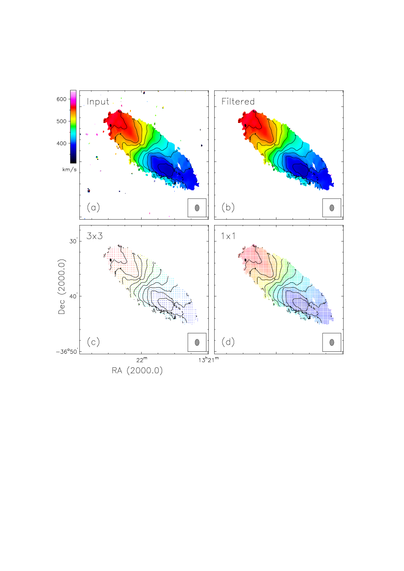
Figure 1.— An example of the pixel sampling mode in 2dbat (LVHIS galaxy NGC 5102): (a) non-filtered and non-sampled ATCA Hi Hermite $h_{3}$ velocity field. The contours are spaced by 20 $\mathrm{km}\,\mathrm{s}^{-1}$, and the synthesized beam is $68.23\,\arcsec\times 43.00\,\arcsec$; (b) the largest connected velocity field passed through the connected-component labelling (CCL) algorithm described in Section 4.1.1; (c) a sampled velocity field with a grid spacing of $3\times 3$ pixels; (d) a sampled velocity field with a grid spacing of $1\times 1$ pixels. The beam size is indicated by the ellipse in the bottom-right corner of each panel.

4.1. Main layout

Through the following three main steps, 2dbat automatically extracts the ring parameters for the 2D tilted-ring model in Eq. 17 given a degree of regularisation.

4.1.1 Mask outlying pixels in the input 2D maps

Outlying pixels that are sporadically distributed in the velocity field and thus have very low likelihood affect the Bayesian fitting in a way that increases the multimodality of the posterior distributions of the parameters (Dawid, 1973). Despite their insignificant contribution to the global kinematics of a galaxy, these outliers often result in larger uncertainties and longer execution time in the fitting process. It is therefore desirable to remove such outliers to minimise their impact on the execution time and the fit quality. To this end, we use the connected-component labelling (CCL) algorithm which finds the largest connected area in a 2D image by masking isolated pixels (Cormen et al., 2009). Using a two-pass procedure, the largest connected region is extracted: (a) in the first pass, scanning from left-to-right and top-to-bottom of the velocity field, successive integers in increasing order starting from number one are temporarily assigned to pixels depending on their connectivity of neighbour pixels. (b) in the second pass, the temporary labels are replaced by the smallest label of its equivalence class, and the connected area with the smallest label is found. We refer to Cormen et al. (2009) for a full description of the algorithm. An example of the extracted largest connected area of the ATCA Hermite $h_{3}$ velocity field of the LVHIS galaxy NGC 5102 (HIPASS J1321-36) (Koribalski et al. submitted) via the CCL algorithm is shown in the panel (b) of Fig. 1.

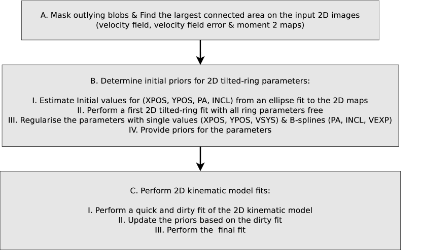
Figure 2.— The main layout of 2dbat. See Section 4.1 for more details.

4.1.2 Optimal range of priors for the ring parameters

multinest requires several input parameters, such as the number of live points $N$, the sampling efficiency $f$, the tolerance level $\epsilon$, and the prior distributions, which all influence the robustness and efficiency of the 2D tilted-ring fitting. The fit quality and the execution time are particularly dependent on the assumed prior distributions of the ring parameters. The prior ranges should cover all the possible values for each of the parameters while being narrowed down in an optimal way. Bayesian fit with optimal prior distributions does not only reduce the execution time but it also avoids any overshooting, leading to more robust results.

We fit an ellipse to the input velocity field to derive a rough parameterisation of the galaxy’s disk on which the estimation of initial values for the geometrical parameters, such as centre position ($x^{\rm ellipse}_{\rm C}$, $y^{\rm ellipse}_{\rm C}$), position angle ($\phi^{\rm ellipse}$), inclination ($i^{\rm ellipse}$) and the length of semi-major axis ($L$_smx) is based. The ellipse fit can also be made to the other moment maps (i.e., moment 0 or 2) if needed. We then perform a first tilted-ring analysis with all ring parameters allowed to vary freely by fitting a model LOS velocity given in Eq. 2.1 to the successive ellipses defined with the ellipse fit above, sub-divided into rings of a minimum width of one beam. The fit results are used for the regularisation of the ring parameters on which their uniform prior distributions are based. We regularise the ring parameters as a function of galaxy radius by performing error-weighted averaging of ($x_{\rm C}$, $y_{\rm C}$, $v_{\rm SYS}$) and fitting of the B-spline functions ($0^{\rm th}$, $1^{\rm st}$, $2^{\rm nd}$ or $3^{\rm rd}$ order) given in Eqs. 10, 11 and 12 for $\phi$, $i$ and $v_{\rm EXP}$, respectively. The regularisation is done by only using the rings satisfying all the following criteria:

$$\overline{\delta^{\rm parameter}_{m}}-5\sigma^{\rm parameter}_{m}<\delta^{\rm parameter}_{m}<\overline{\delta^{\rm parameter}_{m}}+5\sigma^{\rm parameter}_{m},$$ (22)

where $\delta^{\rm parameter}_{m}$ are the statistical uncertainties of the fitted parameters (i.e., $x_{\rm C}$, $y_{\rm C}$, $v_{\rm SYS}$, $\phi$, $i$, and $v_{\rm EXP}$) in each ring ($m=1,...,n$ where $n$ is the number of the rings) derived from the first tilted-ring analysis above, and $\overline{\delta^{\rm parameter}}$ and $\sigma^{\rm parameter}$ are their mean and standard deviation values. We note that this outlier removal process does not much affect the final Bayesian fit results while just providing initial estimates of the priors.

4.1.3 Performing the Bayesian fit of the tilted-ring model

First, we carry out a dirty but quick Bayesian fit of 2D tilted-ring model with a smaller number of live points (e.g., $N=50$) and less-conservative tolerance (e.g., 0.3) and sampling efficiency (0.8) assuming the initial, conservative uniform priors of the ring parameters given in Table 1. These initial prior distributions are further tuned in accordance with the results of the dirty fit. We then apply the full Bayesian model fit with the given parameter setup and the degree of the regularisation. Lastly, we derive the final rotation velocity $v_{\rm ROT}$ by fitting the LOS model velocities to the receding, approaching and both sides of the tilted-rings defined with the parameters from the full Bayesian fitting.

2dbat results include (1) an ascii text file containing the rotation curves and the fitted ring parameters, (2) standard posterior sample files by multinest, (3) model velocity fields constructed using the best fits of the 2D tilted-ring analysis, (4) residual maps between the input and model velocity fields and (5) a weighted 2D error map of the velocity field which is described in the following Section. A schematic flowchart describing the main layout of 2dbat is shown in Fig. 2.

Table 1Initial uniform prior distributions of parameters

Parameter	Min	Max
(1)	(2)	(3)
$x_{\rm C}$	$x^{\rm TR}_{\rm C}-0.5L_{\rm smx}$	$x^{\rm TR}_{\rm C}+0.5L_{\rm smx}$
$y_{\rm C}$	$y^{\rm TR}_{\rm C}-0.5L_{\rm smx}$	$y^{\rm TR}_{\rm C}+0.5L_{\rm smx}$
$v_{\rm SYS}$	$v^{\rm TR}_{\rm SYS}-\sigma^{v_{\rm LOS}}$	$v^{\rm TR}_{\rm SYS}+\sigma^{v_{\rm LOS}}$
$c^{\phi}_{u}\{u=1,...U\}$	$c^{\phi\_{\rm TR}}_{{\it u}}-5\sigma^{c^{\phi\_{\rm TR}}}_{{\it u}}$	$c^{\phi\_{\rm TR}}_{{\it u}}+5\sigma^{c^{\phi\_{\rm TR}}}_{{\it u}}$
$c^{i}_{v}\{v=1,...V\}$	$c^{i\_{\rm TR}}_{{\it v}}-5\sigma^{c^{i\_{\rm TR}}}_{{\it v}}$	$c^{i\_{\rm TR}}_{{\it v}}+5\sigma^{c^{i\_{\rm TR}}}_{{\it v}}$
$c^{v_{\rm EXP}}_{w}\{w=1,...W\}$	$c^{v_{\rm EXP\_TR}}_{{\it w}}-5\sigma^{c^{v_{\rm EXP\_TR}}}_{{\it w}}$	$c^{v_{\rm EXP\_TR}}_{{\it w}}+5\sigma^{c^{v_{\rm EXP\_TR}}}_{{\it w}}$
$n$	0	3$n^{\rm TR}$
$r_{-2}$	0	3$r^{\rm TR}_{-2}$
$\rho_{-2}$	0	3$\rho^{\rm TR}_{-2}$

(1): Parameters of 2D tilted-ring model given in Eq. 17; (2)(3): Default boundaries of the uniform priors of the parameters: Super-script ‘TR’ indicates the values derived from the intial tilted-ring fit; $\rm L_{\rm smx}$ (the length of the semi-major axis); $\sigma^{v_{\rm LOS}}$ (1$\sigma$ of the $v_{\rm LOS}$ distribution); $n^{\rm TR}$, $r^{\rm TR}_{-2}$, and $\rho^{\rm TR}_{-2}$ are derived by fitting the Einasto rotation velocity given in Eq. 16 to the initial rotation velocity $v_{\rm ROT}^{\rm TR}$. See Section 4.1 for more details.

4.2. Error estimation

We adopt the standard deviations of the posterior distributions of the parameters as their errors except for $v_{\rm ROT}$. As discussed above, in the last step of the algorithm, only the final rotation velocity $v_{\rm ROT}$ is fitted to the tilted-rings defined with the other ring parameters derived from the last Bayesian fit. Therefore, the uncertainties of the other ring parameters are not fully incorporated in the standard deviation of $v_{\rm ROT}$ derived in the final fit. As discussed in de Blok et al. (2008) (see also Swaters 1999), such formal standard deviations of $v_{\rm ROT}$ ($\rm\sigma^{{\it v}_{\rm ROT}}_{\it m}$ where $m$ is a ring number from $1$ to $n$) do not represent the true physical uncertainties, and are usually much smaller than the dispersions of LOS velocities along the rings. Following Swaters (1999) and de Blok et al. (2008), 2dbat also provides three types of uncertainties for $v_{\rm ROT}$: (1) the error in $v_{\rm E}$, $\sigma_{v_{\rm E}}$, (2) $\sigma_{\rm asym}$ (a pseudo-$1\sigma$ uncertainty due to asymmetries as one fourth of the difference between the approaching and receding side velocities; see de Blok et al. 2008), and (3) $\sigma_{\rm LOS}$ (the average velocity dispersion along the rings). $\sigma_{v_{\rm E}}$ is associated with the errors of the Einasto halo profile, $n$, $r_{-2}$ and $\rho_{-2}$, which is given by

$$\sigma_{v_{\rm E}} =\Biggl{[}{(\sigma_{n}}\frac{\partial v_{\rm E}}{\partial n})^{2}+(\sigma_{r_{\rm-2}}\frac{\partial v_{\rm E}}{\partial r_{\rm-2}})^{2}+(\sigma_{\rho_{\rm-2}}\frac{\partial v_{\rm E}}{\partial\rho_{\rm-2}})^{2}$$ (23)

$$+2\frac{\partial v_{\rm E}}{\partial n}\frac{\partial v_{\rm E}}{\partial r_{-2}}\sigma_{nr_{-2}}+2\frac{\partial v_{\rm E}}{\partial r_{-2}}\frac{\partial v_{\rm E}}{\partial\rho_{-2}}\sigma_{r_{-2}\rho_{-2}}$$

$$+2\frac{\partial v_{\rm E}}{\partial n}\frac{\partial v_{\rm E}}{\partial\rho_{-2}}\sigma_{n\rho_{-2}}\Biggr{]}^{\!1/2}$$

where $\sigma_{n}$, $\sigma_{r_{-2}}$, and $\sigma_{\rho_{-2}}$ are the standard deviations of the fitted $n$, $r_{-2}$ and $\rho_{-2}$ of the Einasto halo rotation velocity from the Bayesian analysis. $\sigma_{nr_{-2}}$, $\sigma_{r_{-2}\rho_{-2}}$, and $\sigma_{n\rho_{-2}}$ are the covariances between the parameters. The full derivation of the error propagation for the Einasto halo model is given in the Appendix. From this, one can define the uncertainties in the rotation curves by adding either two of the above three uncertainties or even all of them in quadrature as a ’very’ conservative error budget.

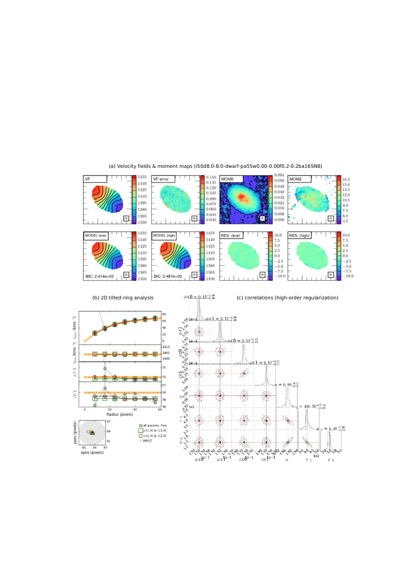
Figure 3.— 2dbat analysis for an artificial dwarf galaxy: (a) hermite $h_{3}$ velocity field, error, moment maps, model and residual velocity fields. Contours are spaced by 10 $\mathrm{km}\,\mathrm{s}^{-1}$ in the velocity fields, 4 $\mathrm{km}\,\mathrm{s}^{-1}$ in both the moment 2 and residual velocity fields, and 0.1 $\rm mJy\,beam^{-1}$ in the moment 0. The beam size is indicated by the ellipse in the bottom-right corner of each panel. The BIC values derived from the Bayesian fits for the model velocity fields are denoted in the panels of model velocity fields, respectively; (b) 2D tilted-ring analysis: the rotation curves derived using the Hermite $h_{3}$ velocity field in the two regularisation modes (green open squares: constant, brown open circles: higher-order B-splines, grey filled circles: fit results with all the ring parameters free, orange cross mark: the input ring parameters used for contructing the model data cube). See Section 5.1.1 for more details; (c) correlations of the ring parameters: the black contours and histograms show the posterior constraints from the Bayesian analysis. The best fits are indicated by red lines.

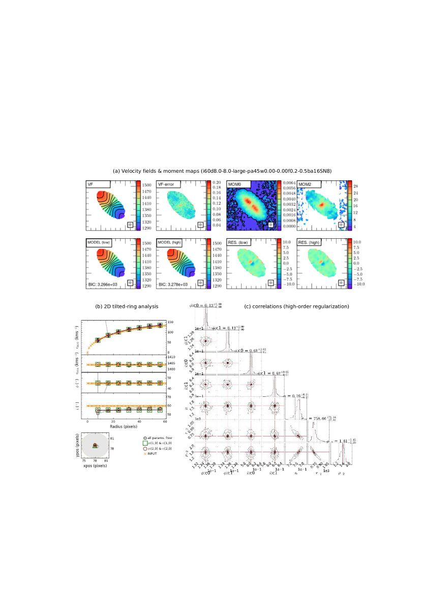
Figure 4.— 2dbat analysis for an artificial intermediate-mass galaxy: (a) hermite $h_{3}$ velocity field, error, moment maps, model and residual velocity fields. Contours are spaced by 20 $\mathrm{km}\,\mathrm{s}^{-1}$ on the velocity fields, 4 $\mathrm{km}\,\mathrm{s}^{-1}$ on both the moment 2 and residual velocity fields, and 0.1 $\rm mJy\,beam^{-1}$ on the moment 0. The beam size is indicated by the ellipse in the bottom-right corner of each panel. The BIC values derived from the Bayesian fits for the model velocity fields are denoted in the panels of model velocity fields, respectively; (b) 2D tilted-ring analysis- the rotation curves derived using the Hermite $h_{3}$ velocity field in the two regularisation modes (green open squares: constant, brown open circles: higher-order B-splines, grey filled circles: fit results with all the ring parameters free, orange cross mark: the input ring parameters used for contructing the model data cube). See Section 5.1.1 for more details; (c) correlations of the ring parameters- the black contours and histograms show the posterior constraints from the Bayesian analysis. The best fits are indicated by red lines.

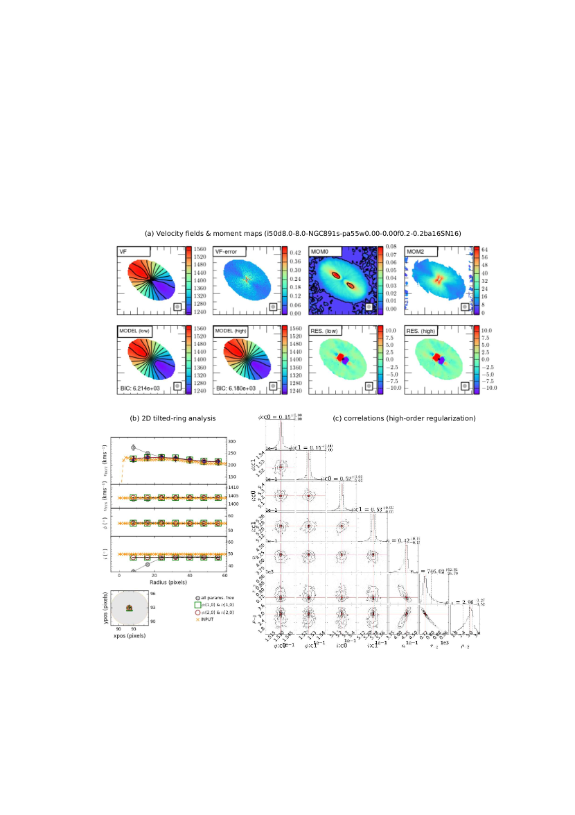
Figure 5.— 2dbat analysis for an artificial massive galaxy: (a) hermite $h_{3}$ velocity field, error, moment maps, model and residual velocity fields. Contours are spaced by 30 $\mathrm{km}\,\mathrm{s}^{-1}$ in the velocity fields, 20 $\mathrm{km}\,\mathrm{s}^{-1}$ in both the moment 2 and residual velocity fields, and 0.1 $\rm mJy\,beam^{-1}$ in the moment 0. The beam size is indicated by the ellipse in the bottom-right corner of each panel. The BIC values derived from the Bayesian fits for the model velocity fields are denoted in the panels of model velocity fields, respectively; (b) 2D tilted-ring analysis: the rotation curves derived using the Hermite $h_{3}$ velocity field in the two regularisation modes (green open squares: constant, brown open circles: higher-order B-splines, grey filled circles: fit results with all the ring parameters free, orange cross mark: the input ring parameters used for contructing the model data cube). See Section 5.1.1 for more details; (c) correlations of the ring parameters: the black contours and histograms show the posterior constraints from the Bayesian analysis. The best fits are indicated by red lines.

4.3. Improving the processing time

As presented in Fig. 1, 2dbat provides a pixel sampling mode in which the velocity field is sampled with a grid spacing in units of pixels supplied by the user. Although some spatial information is lost (see the panels (c) and (d) in Fig. 1), this option is useful for reducing the processing time which increases significantly with the number of pixels to be fitted in the Bayesian analysis. As will be shown in Fig. A-2.1, for well-resolved galaxies, the fit results derived with sampling options where the grid spacing is comparable to or less than the size of one beam are in general agreement with that derived with the full resolution while improving the execution time significantly.

In addition 2dbat has been developed to fully support the built-in Message-Passing Interface (MPI) routines in multinest by which the Bayesian analysis can be parallelized. This enables us to improve the processing time significantly on either a multi-core single or cluster system.

5. Performance test and discussion

In this Section, we test the performance of 2dbat using real data from LVHIS (Koribalski, 2010) as well as artificial galaxies resembling rotation curves of intermediate-mass and massive spiral galaxies which were also used to test fat in Kamphuis et al. (2015).

5.1. Artificial galaxies

We first apply 2dbat to the 52 artificial galaxies in Kamphuis et al. (2015) to assess its performance by comparing the recovered ring parameters with those used for constructing the model galaxies. Kamphuis et al. (2015) built the data cubes of the model galaxies using two representative rotation curves of intermediate-mass and massive spiral galaxies as well as a solid body-like rotation curve of dwarf galaxies. They mimic the surface brightness of the galaxies by locally perturbing an exponential profile with a scale length of 10 kpc which is decreased by a factor of 20 depending on the size of the galaxies. The data cubes for the three base model galaxies are constructed by (1) distributing the flux based on the surface brightness profiles over the velocity ranges spaced by a channel resolution of 4 $\mathrm{km}\,\mathrm{s}^{-1}$, (2) adding white noise, and (3) smoothing them with a Gaussian beam with FWHM of 30″. The beam size is comparable to that of the core of ASKAP at 21cm. In addition, warps are included in the cubes by radially varying the angular momentum vector of the initial disk. Lastly, by varying the size, inclination, position angle, velocity dispersion, angular momentum vector, scale height, S/N, and rotation curve of the three base model galaxies, they ended up with 52 model data cubes.

We extract the velocity fields from the artificial data cubes to which 2D kinematic tilted-ring models are fitted using 2dbat. For this, we fit a third-order Gauss-Hermite polynomial to individual velocity profiles of the data cubes. As discussed in Oh et al. (2011), this allows us to derive more reliable central velocities of the profiles even with significant asymmetries compared to other types of velocity fields, such as moment 1, single Gaussian, or peak velocity fields. As examples, we present the extracted Hermite $h_{3}$ velocity fields of artificial dwarf, intermediate-mass, and massive galaxies together with their moment maps (moment 0 and 2) in panel (a) of Figs. 3 to 5. We note that their zeroth moment maps are not used for the 2dbat analysis but only for showing the integrated intensity of Hi in the galaxies.

5.1.1 Fit results

We run 2dbat on the extracted Hermite $h_{3}$ velocity fields of the 52 artificial galaxies to derive their 2D tilted-ring parameters given the degree of regularisation in a fully automated manner. For $\phi$ and $i$ (or $v_{\rm EXP}$ which is set to zero in this work) whose radial changes can be regularised by B-splines in the 2D galaxy kinematics model, we use two different regularisation modes (constant or high order) which can be specified by the number of knots and spline order ($n$, $k$) as described in Section 3.1. For constant $\phi$ and $i$, we set $\phi^{\rm SPLINE}$($n=1$, $k=0$) and $i^{\rm SPLINE}$($n=1$, $k=0$), respectively. Meanwhile, for the high orders of $\phi$ and $i$, we set $\phi^{\rm SPLINE}$($n=2$, $k=0$) and $i^{\rm SPLINE}$($n=2$, $k=0$), depending on the complexity of their radial variations. The fitting setup of the 2dbat runs adopted for this test is given in Table 2. For each artificial galaxy, we apply 2dbat using the two regularisation modes, resulting in 104 rotation curves in total of the 52 model galaxies. Instead of showing all the fit results of the artificial galaxies, we present those of three representative dwarf, intermediate-mass and massive galaxies in Figs 3 to 5.

Table 2Parameter setup for the performance test of 2dbat

Parameter	Variation
(1)	(2)
sampling
Ring width	1 beam
(RAgrid, RAgrid)	(0.3 beam, 0.3 beam)
(Decgrid, Decgrid)	(0.3 beam, 0.3 beam)
(RA${}^{\rm D}_{\rm grid}$, RA${}^{\rm D}_{\rm grid}$)	(0.3 beam, 0.3 beam)
(Dec${}^{\rm D}_{\rm grid}$, Dec${}^{\rm D}_{\rm grid}$)	(0.3 beam, 0.3 beam)
regularisation
$\phi$ (knots, spline order $k$)	(1, $k=0,1,2$ and $3$)
$i$ (knots, spline order $k$)	(1, $k=0$ and $1$)
$v_{\rm EXP}$ (knots, spline order $k$)	fixed to zero
weight
$|\cos\theta|^{t}$	$t=1$
Free angle around the minor axis	$10^{\circ}$
multinest parameters
N	200 (50 for dirty fits)
efr	0.8
tol	0.1 (0.3 for dirty fits)
maximum iteration	$\infty$

(1): Parameters of 2dbat and multinest. The radial velocities within the free angle are discarded. Super-script ’D’ indicates the parameters for the intial ’dirty’ Bayesian fit. See Section 4.1 for more details.

For each galaxy, we show (1) moment maps + velocity fields, (2) 2D tilted-ring analysis, and (3) correlations between the ring parameters derived. As an example, Fig. 3 shows 2dbat fit results for a well-sampled ($\sim$$7$ beams across the semi-major axis) intermediate mass galaxy with $\phi=55^{\circ}$ and $i=50^{\circ}$. In the top panel (a), its moment maps and input Hermite $h_{3}$ velocity field are presented together with the residual maps and the model velocity fields which are derived using the fit results with the two regularisation setup (i.e., constant or high-order $\phi$ and $i$). The corresponding Bayesian Information Criteria (BIC) statistics values from the fits in the two regularisation modes are also denoted on the model velocity fields, respectively.

In all of the panels for 2D tilted-ring analysis, the ring parameters and rotation curves derived using 2dbat are plotted as open squares, circles, and grey dots connected by solid lines. The grey dots indicate the fit results made with all ring parameters free. These unsupervised fits allow us to check how the radial scatter of the individual ring parameters behaves in general. We also overplot the input ring parameters and rotation curves as indicated by thick dashed lines in the figures, respectively. The correlation panel (c) shows the marginalized posterior distributions of the ring parameters derived in the high-order regularisation setup of $\phi$ (cubic) and $i$ (linear) as adopted in the test.

In the following sections, we compare (1) the derived ring parameters, (2) rotation curves, and (3) model velocity fields produced using the best fit results with those that were used to build the model galaxies. From this, we examine how well 2dbat is able to recover the input ring parameters of the artificial galaxies in the 2D tilted-ring parameter space. Figs. 6 and 7 show the comparison between the model’s input and 2dbat’s output parameters derived assuming constant and high-order regularisations of $\phi$ and $i$ of all the artificial galaxies, respectively. As shown in the figures, the fit results derived in the two different regularisation modes are robust and largely consistent with each other within the scatter.

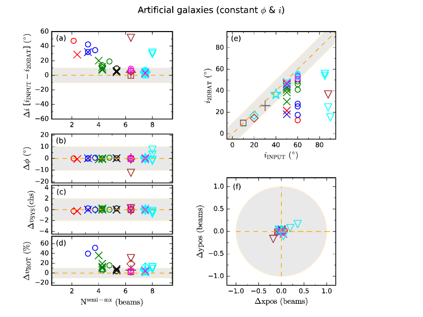
Figure 6.— Comparison of the fit results between 2dbat and the input ones (constant $\phi$ and i): (a) inclination $i$ offset against the number of resolved elements $\rm N^{\rm semi-mx}$ across the semi-major axis. Different symbols denote the range of the derived inclinations ($20^{\circ}\--70^{\circ}$) in steps of $10^{\circ}$. The grey shaded region indicates $\pm 10^{\circ}$ offset; (b) position angle offset, $\Delta\phi$ ($\phi_{\rm INPUT}-\phi_{\rm 2DBAT}$) in degrees against $\rm N^{\rm semi-mx}$; (c) Systemic velocity offset $\Delta v_{\rm SYS}$ ($v_{\rm SYS}^{\rm INPUT}-v_{\rm SYS}^{\rm 2DBAT}$) in units of the channel resolution against $\rm N^{\rm semi-mx}$; (d) rotation velocity offset $\Delta v_{\rm ROT}$ against $\rm N^{\rm semi-mx}$. $\Delta v_{\rm ROT}$ is calculated as $(v_{\rm ROT}^{\rm INPUT}-v_{\rm ROT}^{\rm 2DBAT})/v_{\rm ROT}^{\rm Max}$ where $v_{\rm ROT}^{\rm Max}$ is the input maximum rotation velocities; (e) one-to-one comparison of the inclinations between the input values and those derived using 2dbat. The grey shaded region indicates $\pm 10^{\circ}$ offset with respect to the line of equality (dashed line); (f) centre position offset in beam size. The grey shaded region indicates one beam size centred on the input kinematic centre positions.

$\bullet$ $\Delta i:$ The inclination difference, $\Delta i$ ($i_{\rm INPUT}-i_{\rm 2DBAT}$) of the model galaxies is shown in the panels (a) against the number of resolved elements across the semi-major axis, $\rm N^{\rm semi-mx}$, together with a direct one-to-one comparison between them as given in the panels (e). The input inclination values are shown by different symbols in steps of $10^{\circ}$, from $10^{\circ}$ to $90^{\circ}$ in the panels (e) of Figs. 6 and 7. $\Delta i$ values are grouped into bins from 2 to 8 beams as represented with different colours in the same panels. On the whole, the derived inclinations by 2dbat are in good agreement with the input ones within $\sim$$10^{\circ}$ for the galaxies with $10<i<70^{\circ}$ with more than four resolution elements across the semi-major axis.

Interestingly, 2dbat provides reliable estimates of inclinations even for face-on-like galaxies with inclinations of $10$ and $20^{\circ}$ as long as their velocity fields are well-sampled (i.e., $\rm N^{\rm semi-mx}>5$), regular and symmetric in shape. However, the fit results show a trend of increasing $\Delta i$ towards decreasing $\rm N^{\rm semi-mx}$ as colour-coded in the panels (a). The inclination offset is most prominent at the smallest $\rm N^{\rm semi-mx}<3$. The majority of the galaxies with $\rm N^{\rm semi-mx}<5$ show large inclination offsets ($>10^{\circ}$) although they have intermediate inclinations with $50$ or $60$ degrees. This can be mainly attributed to beam smearing. As discussed earlier, it usually results in more parallel iso-velocity contours across the velocity field which are modelled using a lower inclination in the 2D fit. This is the case of the galaxies with $\rm N^{\rm semi-mx}<5$ in panel (a) which seem to be significantly affected by the beam smearing. A similar trend of increasing $\Delta i$ with decreasing $\rm N^{\rm semi-mx}$ is also found in Kamphuis et al. (2015) where the same artificial galaxies are used for the tilted-ring analysis in a three-dimensional way although it is only significant at $\rm N^{\rm semi-mx}<3$. Meanwhile, regardless of $\rm N^{\rm semi-mx}$, for edge-on-like galaxies with $i>80^{\circ}$, the offsets are very large ($>40^{\circ}$), due to less data points to be fitted in given rings and the projection effect of line-of-sight velocities in the galaxies. This shows that either the lower sampling of velocity fields or the higher degeneracy between $v_{\rm ROT}$ and $i$, or both are mainly responsible for such large inclination offsets in face-on, and edge-on galaxies or even in galaxies with intermediate inclinations but with poor sampling. Together with beam smearing, this is a fundamental limitation of 2D tilted-ring analysis.

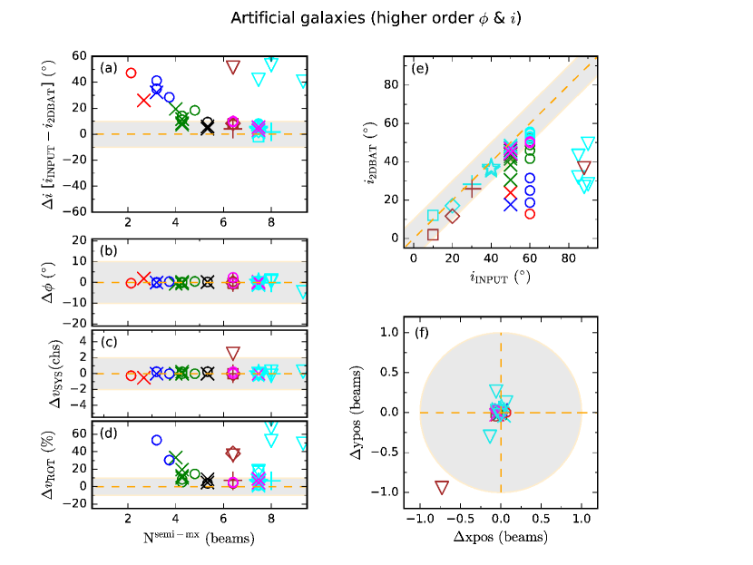
Figure 7.— Comparison of the fit results between 2dbat and the input ones (higher order $\phi$ and i): (a) inclination $i$ offset against the number of resolved elements $\rm N^{\rm semi-mx}$ across the semi-major axis. Different symbols denote the range of the derived inclinations ($20^{\circ}\--70^{\circ}$) in steps of $10^{\circ}$. The grey shaded region indicates $\pm 10^{\circ}$ offset; (b) position angle offset, $\Delta\phi$ ($\phi_{\rm INPUT}-\phi_{\rm 2DBAT}$) in degrees against $\rm N^{\rm semi-mx}$; (c) Systemic velocity offset $\Delta v_{\rm SYS}$ ($v_{\rm SYS}^{\rm INPUT}-v_{\rm SYS}^{\rm 2DBAT}$) in units of the channel resolution against $\rm N^{\rm semi-mx}$; (d) rotation velocity offset $\Delta v_{\rm ROT}$ against $\rm N^{\rm semi-mx}$. $\Delta v_{\rm ROT}$ is calculated as $(v_{\rm ROT}^{\rm INPUT}-v_{\rm ROT}^{\rm 2DBAT})/v_{\rm ROT}^{\rm Max}$ where $v_{\rm ROT}^{\rm Max}$ is the input maximum rotation velocities; (e) one-to-one comparison of the inclinations between the input values and those derived using 2dbat. The grey shaded region indicates $\pm 10^{\circ}$ offset with respect to the line of equality (dashed line); (f) centre position offset in beam size. The grey shaded region indicates one beam size centred on the input kinematic centre positions.

Table 3Observational properties of LVHIS sample galaxies

HIPASS ID	NED ID	$\alpha$ (J2000)	$\delta$ (J2000)	$v_{\rm SYS}$	$\phi$	$i$	D	$\Theta_{\rm MX}$	Fig#
		(hh:mm:ss)	(dd:mm:ss)	($\mathrm{km}\,\mathrm{s}^{-1}$)	(∘)	(∘)	(Mpc)
(1)	(2)	(3)	(4)	(5)	(6)	(7)	(8)	(9)	(10)
HIPASS J1441-62		14 41 37	-62 44 38	672$\pm$8				1.75	A-2.1
HIPASS J1305-40	CEN 06	13 05 02	-40 06 30	617$\pm$4		60	6.1	2.38	A-2.2
HIPASS J0320-52	NGC 1311	03 20 05	-52 11 34	568$\pm$5	40	79$\pm$1	5.3	3.69	A-2.3
HIPASS J1337-39		13 37 30	-39 52 56	492$\pm$4		36	4.8	4.29	A-2.4
HIPASS J1219-79	IC 3104	12 19 04	-79 42 55	429$\pm$4	45	59$\pm$6	2.6	4.48	A-2.5
HIPASS J1047-38	ESO 318-G013	10 47 39	-38 51 45	711$\pm$7	75	$\geq 88$		4.65	A-2.6
HIPASS J1428-46	UKS 1424-460	14 28 06	-46 18 32	390$\pm$2		73	3.4	4.88	A-2.7
HIPASS J1620-60	ESO 137-G018	16 20 56	-60 29 18	605$\pm$3	30	73$\pm$2	5.9	5.35	A-2.8
HIPASS J0705-58	AM 0704-582	07 05 18	-58 31 19	564$\pm$2		65	4.9	5.63	A-2.9
HIPASS J1337-28	ESO 444-G084	13 37 18	-28 02 17	587$\pm$3		39$\pm$4	5.1	6.21	A-2.10
HIPASS J0731-68	ESO 59-G001	07 31 20	-68 11 19	530$\pm$3		20$\pm$18	4.5	6.39	A-2.11
HIPASS J0333-50	IC 1959	03 33 15	-50 25 17	640$\pm$4	147	88$\pm$4	8.2	6.55	A-2.12
HIPASS J1403-41	NGC 5408	14 03 21	-41 22 26	506$\pm$3	62	55$\pm$8	4.9	6.87	A-2.13
HIPASS J1337-42	NGC 5237	13 37 47	-42 50 51	361$\pm$4	128	35$\pm$0	3.7	7.92	A-2.14
HIPASS J1348-53	ESO 174-G?001	13 48 01	-53 21 31	688$\pm$3	170	76$\pm$11		10.41	A-2.15
HIPASS J1057-48	ESO 215-G?009	10 57 32	-48 11 02	598$\pm$2	72	64$\pm$27	5.3	11.86	A-2.16
HIPASS J1501-48	ESO 223-G009	15 01 08	-48 17 04	588$\pm$2	135	44$\pm$19	6.0	11.92	A-2.17
HIPASS J2202-51	IC 5152	22 02 41	-51 17 37	122$\pm$2	100	51$\pm$4	1.8	12.78	A-2.18
HIPASS J0256-54	ESO 154-G023	02 56 55	-54 34 58	574$\pm$2	39	$\geq 88$	6.8	13.30	A-2.19
HIPASS J1305-49	NGC 4945	13 05 24	-49 29 35	563$\pm$3	43	85$\pm$4	4.1	14.32	A-2.20
HIPASS J1321-36	NGC 5102	13 21 55	-36 38 03	468$\pm$2	48	70$\pm$6	3.4	14.59	A-2.21
HIPASS J0047-25	NGC 253	00 47 31	-25 17 22	243$\pm$2	52	83$\pm$0	3.1	21.50	A-2.22
HIPASS J1413-65	Circinus	14 13 27	-65 18 46	434$\pm$3	40	64$\pm$4	4.2	22.72	A-2.23
HIPASS J0317-66	NGC 1313	03 17 57	-66 33 30	470$\pm$2		36$\pm$7	4.0	42.54	A-2.24

(1)(2): HIPASS and NASA Extra-galactic Database (NED) names; (3)(4): HI centroid derived using a Gaussian fit to moment 0 in Koribalski et al. (2004); (5)(6)(7): Systemic velocities, optical position angle ($\phi$), and optical inclination ($i$) taken from Kamphuis et al. (2015); (8): Distance taken from NED as given in Kamphuis et al. (2015); (9): Number of beams across the morphological major axis derived from an ellipse fit to the velocity field; (10): Figure number in this paper.

$\bullet$ $\Delta\phi$, $\Delta v_{\rm SYS}$, $\Delta v_{\rm ROT}$ and centre position offset: As found in the panels (b), (c), (d), and (f), 2dbat recovers the input $\phi$, $v_{\rm SYS}$ and centre position ($x_{\rm C}$, $y_{\rm C}$) of most of the artificial galaxies with $10^{\circ}<i<70^{\circ}$ with good accuracy: $\Delta\phi<2^{\circ}$; $\Delta v_{\rm SYS}<1$ channel resolution; $\Delta$$x_{\rm C}<1.0$ beam; $\Delta$$y_{\rm C}<1.0$ beam regardless of $\rm N^{\rm semi-mx}$. This shows that 2dbat is able to provide reliable estimates of these weakly correlated parameters in the 2D tilted-ring analysis even for edge-on-like galaxies with $i>80^{\circ}$.

$\bullet$ $\Delta v_{\rm ROT}$: Likewise, for most galaxies, the rotation velocity offsets, $\Delta v_{\rm ROT}$ which are the weighted means of the residuals between the input and derived ones over all the radii given their errors are in general within 10% of the input maximum rotation velocities. The majority positive $\Delta v_{\rm ROT}$ values indicate that the derived rotation velocities are lower than the input ones. This shows that the 2D analysis is affected by beam smearing which tends to lower the intrinsic rotation velocities. The outliers showing more than 10% deviations correspond to face-on galaxies, where small inclination offsets can lead to large offsets in $v_{\rm ROT}$. Meanwhile, the edge-on-like galaxies with $i>70^{\circ}$ also show large $\Delta v_{\rm ROT}$ mainly due to the poor sampling of the velocity field combined with the projection effect which results in significant offsets in inclination. This indicates that 2dbat can be applied to galaxies with $20^{\circ}<i<70^{\circ}$ and at least four resolution elements across the semi-major axis.

As shown in Figs. 3 to 5, regarding the residual maps between the input and model velocity fields (i.e., line-of-sight velocities) reconstructed using the best fit parameters, they are mostly smaller than the channel resolution ($\sim$4 $\mathrm{km}\,\mathrm{s}^{-1}$) for all the artificial galaxies, except for some localized regions where S/N is low. This confirms that the 2D fits themselves were made without any failure as also indirectly supported by the well-defined Gaussian distribution of the posteriors in the correlation plots. Regarding the processing time of 2DBAT, it takes about 10 minutes for a laptop with a standard four-cores processor to fit the kinematic model with constant PA/INCL to the artificial dwarf galaxy shown in Fig. 3. For the sampling option with a grid spacing of a half beam size, the rotation curves are in general agreement with those derived from FAT whose execution time on a similar specified laptop is about 30 minutes.

In summary, for the artificial galaxies with intermediate inclinations ($20\--70^{\circ}$) that are resolved by more than four beams across the semi-major axis, the 2D tilted-ring parameters recovered by 2dbat in a fully automated manner show good agreement with the input ones.

5.2. Real galaxies

We continue to test the performance of 2dbat using sample galaxies taken from LVHIS (Koribalski, 2010). LVHIS is a large Hi survey for a sample of 82 nearby ($<$ 10 Mpc), gas-rich galaxies undertaken with the Australia Telescope Compact Array (ATCA) which aims to investigate fundamental Hi properties and kinematics of the galaxies by providing a comprehensive Hi galaxy atlas.

Of the parent LVHIS sample, we select 24 galaxies which are resolved by more than two independent beams across their major axes and show systematic rotation in their velocity fields. The optical inclinations of the galaxies range from $20^{\circ}$ to $88^{\circ}$. Although some of these are falling outside the reliable fit range of 2dbat (i.e., $\rm N^{\rm semi-mx}>4$ and $20^{\circ}<i<70^{\circ}$) as discussed in Section 5.1.1, we include them to test how well 2dbat is able to perform in marginal cases. These LVHIS galaxies were also manually fitted by rotcur and used to test the performance of fat by Kamphuis et al. (2015). The velocity fields of the resolved galaxies from WALLABY are expected to be more or less like those of the LVHIS sample galaxies, in terms of the spatial ($20$-$60$″) and spectral ($4$ $\mathrm{km}\,\mathrm{s}^{-1}$) resolution as well as the number of resolved elements across the major axis. The basic observational properties of the galaxies, sorted by the number of beams across the morphological major axis are listed in Table 3. We refer to Koribalski et al. (submitted) for more details of the Hi observations and data reduction.

In exactly the same way as the artificial galaxies were analyzed in Section 5.1, we extract the Hermite $h_{3}$ velocity fields from the data cubes of the sample galaxies as well as moment maps (0th and 2nd), and perform a 2D tilted-ring analysis using 2dbat given two regularisation modes of (constant or high-order) $\phi$ and $i$. For the higher level of regularisation, we manually specify the order of B-splines of $\phi$ and $i$ for each galaxy, depending on the number of resolved elements across the major axis and the level of radial change in the ring parameters. The number of knots and the orders of B-spline chosen are denoted in the panel (b) of Figs A-2.1 to A-2.24.

We make a direct comparison between the 2dbat fit results and the ones derived from a 2D tilted-ring analysis using rotcur in GIPSY. The manual rotcur fits were made by regularizing $\phi$ and $i$ with polynomials depending on the degree of their radial scatters on a galaxy-by-galaxy basis. These manual fits are also used in Kamphuis et al. (2015) for a detailed comparison with the 3D method. The extracted velocity fields, moment maps and the reconstructed velocity fields from the 2dbat’s best fits are presented in the Appendix, Figs. A-2.1 to A-2.24, in the same format as for the artificial galaxies. The beam size of the observations is indicated by an ellipse in the bottom-right corner of panels (a).

As with the artificial galaxies, we present the comparisons between the ring parameters derived using both rotcur and 2dbat given the regularisation of $\phi$ and $i$ in Figs. 8 and 9, respectively. We also overplot the fit results made with all ring parameters free as given by grey solid dots. These unsupervised fits allow us to check how the radial scatter of the individual ring parameters behaves in general. In this paper, through the comparison with rotcur, we focus on how the 2dbat fit results are comparable to those manually derived using a standard method of 2D tilted-ring analysis. For a detailed discussion of the comparison of the rotcur results with a 3D method (tirific) as well as another 2D method (diskfit), we refer to Kamphuis et al. (2015).

5.2.1 Fit results

$\bullet$ $\Delta i:$ As shown in the panel (a) of Fig. 8, there may be a trend of increasing $\Delta i$ with decreasing $\rm N^{\rm semi-mx}$ although it is less clear compared to the artificial galaxies. As examples, HIPASS J1441-62 ($\Delta i\sim+40^{\circ}$; open star; Fig. A-2.1), HIPASS J0320-52 ($\Delta i\sim+15^{\circ}$; open circle; Fig. A-2.3), HIPASS J1337-39 ($\Delta i\sim+20^{\circ}$; open circle; Fig. A-2.4), HIPASS J1219-79 ($\Delta i\sim+15^{\circ}$; open star; Fig. A-2.5), and HIPASS J1047-38 ($\Delta i\sim+20^{\circ}$; upside-down triangle; Fig. A-2.6) with $\rm N^{\rm semi-mx}<4$ lie outside the grey shaded region of $\pm 10^{\circ}$ in the panel (a) of Figs. 8 and 9. However, they have intermediate inclinations of $\sim$$40^{\circ}$ according to the manual fit using rotcur somewhat dependent on subjective model choices for the ring parameters. As shown in Figs. A-2.1, A-2.3, A-2.4, A-2.5 and A-2.6, their velocity fields are poorly sampled, smoothing the kinematic structure around the central region. These galaxies are likely to be affected by beam smearing. However, according to the Gaussian-like posterior distributions of the ring parameters as shown in the figures, and the corresponding small amplitudes ($<1$ channel resolution) of the residual maps between the input and model velocity fields, 2dbat seems to provide reasonable fits. The subjective choices of the regularisation in the course of manual tilted-ring analysis using rotcur can induce large values for $\Delta i$.

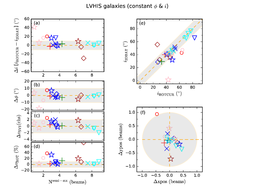
Figure 8.— Comparison of the fit results for the LVHIS galaxies from 2dbat and rotcur (constant $\phi$ and i): (a) inclination $i$ offset against the number of resolved elements $\rm N^{\rm semi-mx}$ across the semi-major axis. Different symbols denote the range of the derived inclinations ($20^{\circ}\--70^{\circ}$) in steps of $10^{\circ}$. The grey shaded region indicates $\pm 10^{\circ}$ offset; (b) position angle offset, $\Delta\phi$ ($\phi_{\rm ROTCUR}-\phi_{\rm 2DBAT}$ in degrees against $\rm N^{\rm semi-mx}$; (c) Systemic velocity offset $\Delta v_{\rm SYS}$ ($v_{\rm SYS}^{\rm ROTCUR}-v_{\rm SYS}^{\rm 2DBAT}$) in units of the channel resolution against $\rm N^{\rm semi-mx}$; (d) rotation velocity offset $\Delta v_{\rm ROT}$ against $\rm N^{\rm semi-mx}$. $\Delta v_{\rm ROT}$ is calculated as $(v_{\rm ROT}^{\rm ROTCUR}-v_{\rm ROT}^{\rm 2DBAT})/v_{\rm ROT}^{\rm Max}$ where $v_{\rm ROT}^{\rm Max}$ is the maximum rotation velocities derived from rotcur; (e) one-to-one comparison between the inclinations derived using 2dbat and rotcur. The grey shaded region indicates $\pm 10^{\circ}$ offset with respect to the line of equality (dashed line); (f) centre position offset in beam size. The grey shaded region indicates one beam size centred on the kinematic centre positions derived using rotcur.

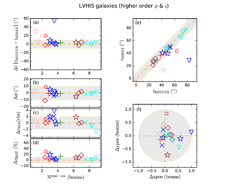
Figure 9.— Comparison of the fit results for the LVHIS galaxies from 2dbat and rotcur (higher order $\phi$ and i): (a) inclination $i$ offset against the number of resolved elements $\rm N^{\rm semi-mx}$ across the semi-major axis. Different symbols denote the range of the derived inclinations ($20^{\circ}\--70^{\circ}$) in steps of $10^{\circ}$. The grey shaded region indicates $\pm 10^{\circ}$ offset; (b) position angle offset, $\Delta\phi$ ($\phi_{\rm ROTCUR}-\phi_{\rm 2DBAT}$ in degrees against $\rm N^{\rm semi-mx}$; (c) Systemic velocity offset $\Delta v_{\rm SYS}$ ($v_{\rm SYS}^{\rm ROTCUR}-v_{\rm SYS}^{\rm 2DBAT}$) in units of the channel resolution against $\rm N^{\rm semi-mx}$; (d) rotation velocity offset $\Delta v_{\rm ROT}$ against $\rm N^{\rm semi-mx}$. $\Delta v_{\rm ROT}$ is calculated as $(v_{\rm ROT}^{\rm ROTCUR}-v_{\rm ROT}^{\rm 2DBAT})/v_{\rm ROT}^{\rm Max}$ where $v_{\rm ROT}^{\rm Max}$ is the maximum rotation velocities derived from rotcur; (e) one-to-one comparison between the inclinations derived using 2dbat and rotcur. The grey shaded region indicates $\pm 10^{\circ}$ offset with respect to the line of equality (dashed line); (f) centre position offset in beam size. The grey shaded region indicates one beam size centred on the kinematic centre positions derived using rotcur.

As more extreme examples, HIPASS J1047-38 ($\Delta i\sim-20^{\circ}$; open circle; see Fig. A-2.6), HIPASS J1305-40 ($\Delta i\sim+20^{\circ}$; open star; ), and HIPASS J1441-62 ($\Delta i\sim-30^{\circ}$; open star) with $\rm N^{\rm semi-mx}<2$ lie outside the grey shaded region of $\pm 10^{\circ}$ in the panel (a) of Figs. 8 and 9. However, they have intermediate inclinations of $\sim$$65^{\circ}$ according to the manual fit using rotcur although again somewhat dependent on subjective model choices for the ring parameters. As shown in Figs. A-2.6, A-2.16 and A-2.20, their velocity fields are poorly sampled, smoothing the kinematic structure around the central region. These galaxies are even more likely to be affected by beam smearing. However, according to the Gaussian-like posterior distributions of the ring parameters as shown in Figs. A-2.6, A-2.16 and A-2.20, and the corresponding small amplitudes ($<1$ channel resolution) of the residual maps between the input and model velocity fields, 2dbat again seems to provide reasonable fits.

On the other hand, the amplitudes of $\Delta i$ are in general reduced if the higher order regularisation for $\phi$ and $i$ is used. This is because the high-order regularisation mode usually provides a better kinematic description of most galaxies than the constant regularisation mode in terms of the fit quality. As shown in Fig. A-2.17, HIPASS J1501-48 is one such galaxy where significant radial variations of $\phi$ and $i$ are shown in their velocity fields. In a more quantitative sense, this is also supported by the smaller value of BIC in the high-order regularisation mode. We emphasize that the number of knots and orders of B-spline for $\phi$ and $i$ were chosen to avoid any significant overfit in the high-order regularisation mode.

The inclinations of HIPASS J1047-38 (ESO 318-G013) and HIPASS J0333-50 derived using both rotcur and 2dbat are comparable with each other but show significant difference ($>30^{\circ}$) compared to the ones calculated from their optical axis ratios. There may be intrinsic difference between the kinematic and photometric geometries of the galaxies, resulting in such large inclination offsets. Or it could be due to the low spatial sampling of the velocity fields given that the kinematic $\phi$ are close to the optical ones. As shown in the panels (a) of Figs. A-2.6 and A-2.12, the iso-velocity contours seen in the velocity fields are predominantly parallel to the minor axes. Such iso-velocity contours often originate from either kinematic or observational characteristics of galaxies, such as solid body-like rotations (Wright, 1974), co-rotating disks of edge-on galaxies, significant expansion velocities (Begum & Chengalur, 2003), beam smearing effects (Teuben, 2002), or bar streaming motions (Wong et al., 2004). For the case of HIPASS J1047-38 (ESO 318-G013) and HIPASS J0333-50, the beam smearing effect appears to be mainly responsible for the parallel iso-velocity contours given the small number of resolved elements ($\rm N^{\rm semi-mx}<3$). As a way to circumvent the beam smearing effect and correct for rotation velocities, the fitting can be made after fixing $\phi$ and $i$ (including the centre position if needed) with the photometric ones derived from optical or infrared observations (e.g., Weldrake et al. 2003). As discussed earlier, this is a fundamental limitation of 2D tilted-ring analysis and is a situation in which the 3D approach may be preferred. For instances, for HIPASS J1047-38 and J0333-50, the 3D fit results from FAT give inclinations of 80 and 85 degrees, respectively, which are more comparable to the optical ones. We refer to Kamphuis et al. (2015) for more discussion on the comparison of the marginally resolved LVHIS galaxies between 2D and 3D tilted-ring analyses.

$\bullet$ $\Delta\phi$, $\Delta v_{\rm SYS}$, $\Delta v_{\rm ROT}$ and centre position: As shown in the panels (b), (c), (d) and (f) in Figs. 8 and 9, 2dbat, in general, provides comparable fit results to the manual fits using rotcur, giving small offsets in $\phi$ ($<2^{\circ}$), $v_{\rm SYS}$ ($<1$ channel resolution) and centre position (within one beam size) except for a few outliers showing $\sim$$10^{\circ}$ offsets mainly in $\phi$. For the outlying galaxies, the fits with higher order regularisation of $\phi$ and $i$ give smaller offsets in $\Delta\phi$. As shown in Fig. A-2.17, the significant radial variation in $\phi$ of HIPASS J1501-48 is better modeled by a cubic B-spline which is also comparable to that derived using rotcur in manual.

$\bullet$ $\Delta v_{\rm ROT}$: The corresponding $\Delta v_{\rm ROT}$, given both the constant and higher order regularisation for $\phi$ and $i$, are mostly within 10% of the maximum rotation velocities of the galaxies with $\rm N^{\rm semi-mx}>5$. As found in the case of the artificial galaxies, there is a similar trend, with offsets at small $\rm N^{\rm semi-mx}$, particularly $\rm N^{\rm semi-mx}<4$. As discussed earlier, inclination offsets caused by the poor sampling of the velocity fields are the major factor that induces such offsets in $v_{\rm ROT}$. As presented in the residual maps between the input and model velocity fields of Figs. A-2.1 to A-2.24, the residual LOS velocities are mostly smaller than 2 $\mathrm{km}\,\mathrm{s}^{-1}$ on average which is less than a half of the channel resolution for the LVHIS data. This indicates that the fits themselves were made without any convergence failure, regardless of the degeneracy between $v_{\rm ROT}$ and $i$ found in the less-resolved and less-inclined galaxies.

In summary, as found in the performance test using the artificial galaxies, 2dbat provides reliable 2D tilted-ring parameters and rotation velocities in a fully automated manner for the LVHIS sample galaxies with intermediate inclinations ($20^{\circ}\--70^{\circ}$) resolved by more than four beams across their semi-major axis. The best fit values and models of centre position, $v_{\rm SYS}$, $\phi$ and $i$ are representative enough to account for their radial scatter seen when a fit is made with all the ring parameters free. Moreover, they are also largely comparable to those derived in manual using rotcur. For most galaxies, higher-order regularisation of $\phi$ and $i$ with the respective B-splines provides a better kinematic description while taking into account the level of radial variations in terms of the calculated BIC statistics. On the other hand, for either the less-resolved ($<$ four beams across the semi-major axis), less or highly-inclined ($<30^{\circ}$ or $>70^{\circ}$) galaxies, the $\phi$ and $i$ derived using 2dbat tend to deviate from the ones calculated from the optical axis ratios although some are comparable to the rotcur results. The enhanced degeneracy between rotation velocity and inclination in such less-resolved, less or highly-inclined galaxies is most likely to be the major reason for the large deviations.

6. Conclusions

In this paper we present a newly developed 2D tilted-ring fitting algorithm based on a Bayesian MCMC technique which allows us to derive 2D tilted-ring parameters and rotation curves of disk galaxies in a fully automated manner. In the algorithm, the ring parameters except for rotation velocity are grouped in two sub-groups, (1) kinematic centre and systemic velocity, and (2) position angle, inclination, and expansion velocity, which are regularised by single values and B-spline functions, respectively. The Einasto halo model rotation velocity comprising three free parameters is used for parameterizing the rotation velocity which is then used together with the other ring parameters for building a 2D kinematic disk model. The disk model is then fitted to the entire region of the input velocity field (without dividing them into individual tilted-rings as in the traditional tilted-ring analysis) in a Bayesian framework at one time. After determining the geometrical ring parameters of the disk model, such as kinematic centre, position angle and inclination, the final rotation velocities are fitted to the tilted-rings defined with the derived geometrical parameters.

For the 2D Bayesian model fitting, we have developed a standalone software written in C, the so-called 2dbat which employs multinest (Feroz & Hobson, 2008; Feroz et al., 2009b, 2013), a Bayesian inference tool library implementing the nested sampling algorithm. multinest has been found to be efficient and robust in calculating the posterior distribution and the evidence for a given likelihood function, even in high dimensions, and successfully used in a wide range of astrophysical inference problems. The most important advantage of 2dbat based on the Bayesian MCMC analysis is that only broadly defined ranges are required for the prior of each ring parameter, which makes the fitting procedure fully automated.

To improve the fit quality and reduce the processing time, it includes some pre-processing steps, such as (1) masking outlying pixels out in the input velocity field and (2) providing initial priors. 2dbat then derives the best fits of the ring parameters by calculating the maximum likelihood estimates of 2D kinematic models for a given 2D velocity field. To further minimise the processing time, it is written in MPI, which ensures the parallel implementation of the multinest on either a multi-core single or cluster system.

We test 2dbat on the Hermite $h_{3}$ velocity fields of 24 LVHIS sample galaxies (Koribalski, 2010) as well as 52 artificial galaxies presented in Kamphuis et al. (2015) using two regularisation regimes (constant or high-order $\phi$ and $i$), and derive (1) 2D tilted-ring parameters, (2) rotation curves and (3) model velocity fields. The fit results are then compared with those that were used to construct the artificial galaxies and those derived using rotcur in GIPSY by hand for the LVHIS sample galaxies, respectively. From this, we found that, for the galaxies with moderate inclinations ($20^{\circ}\--70^{\circ}$) resolved by more than four beams across the semi-major axis, 2dbat is able to provide robust and acceptable fits of 2D kinematic models in a fully automated manner which are well consistent with either the input models or the ones derived manually. 2dbat is limited in breaking the degeneracy between rotation velocity and inclination in the 2D tilted-ring model for poorly sampled ($<4$ beams) galaxies as well as galaxies outside the range $20^{\circ}\--70^{\circ}$. These suffer the greatest from the beam smearing effect. This limitation of 2D tilted-ring analysis would be improved by expanding the current 2D parameter space of 2dbat to the 3D one in a Bayesian framework.

Together with fat which is based on tirific, 2dbat will be useful for robust kinematic analysis of a large number of galaxies from the upcoming SKA pathfinder galaxy surveys, such as ASKAP WALLABY and also from other spectral line observations including optical integral field unit (IFU) spectroscopic or CO observations.

A.1. Error propagation of the Einasto halo rotation velocity

In this Appendix, we provide an error propagation for the three parameters of the Einasto halo rotation velocity in Eq. 16, which is given as,

$$v_{\rm E}(r) =\sqrt{\frac{GM_{\rm E}(r)}{r}}$$

$$=\sqrt{4\pi Gn\frac{r^{3}_{-2}}{r}\rho_{-2}e^{2n}(2n)^{-3n}\gamma(3n,\frac{r}{r_{-2}})}.$$ (A-1.1)

We compute the total uncertainty in $v_{\rm E}(r)$, $\sigma_{v_{\rm E}}$ which is propagated from the 1$\sigma$ errors ($\sigma_{n}$, $r_{\rm-2}$, and $\sigma_{\rho_{\rm-2}}$) of the thee parameters derived from 2dbat as follows:

$$\sigma_{v_{\rm E}} =\sqrt{{(\sigma_{n}}\frac{\partial v_{\rm E}}{\partial n})^{2}+(\sigma_{r_{\rm-2}}\frac{\partial v_{\rm E}}{\partial r_{\rm-2}})^{2}+(\sigma_{\rho_{\rm-2}}\frac{\partial v_{\rm E}}{\partial\rho_{\rm-2}})^{2}+2\frac{\partial v_{\rm E}}{\partial n}\frac{\partial v_{\rm E}}{\partial r_{-2}}\sigma_{nr_{-2}}+2\frac{\partial v_{\rm E}}{\partial r_{-2}}\frac{\partial v_{\rm E}}{\partial\rho_{-2}}\sigma_{r_{-2}\rho_{-2}}+2\frac{\partial v_{\rm E}}{\partial n}\frac{\partial v_{\rm E}}{\partial\rho_{-2}}\sigma_{n\rho_{-2}}}$$ (A-1.2)

where $\sigma_{n}$, $\sigma_{r_{-2}}$, and $\sigma_{\rho_{-2}}$ are the standard deviations of the fitted $n$, $r_{-2}$ and $\rho_{-2}$ of the Einasto halo rotation velocity from the Bayesian analysis. $\sigma_{nr_{-2}}$, $\sigma_{r_{-2}\rho_{-2}}$, and $\sigma_{n\rho_{-2}}$ are the covariances between the parameters which are given by

$$\sigma_{nr_{-2}}=\frac{1}{N}\sum_{i=1}^{N}(n^{i}-n)(r_{-2}^{i}-r_{-2}),$$ (A-1.3)

$$\sigma_{r\rho_{-2}}=\frac{1}{N}\sum_{i=1}^{N}(r_{-2}^{i}-r_{-2})(\rho_{-2}^{i}-\rho_{-2}),$$ (A-1.4)

$$\sigma_{n\rho_{-2}}=\frac{1}{N}\sum_{i=1}^{N}(n^{i}-n)(\rho_{-2}^{i}-\rho_{-2}).$$ (A-1.5)

In addition, the partial derivatives of $v_{\rm E}$ with respect to $n$, $r_{-2}$, and $\rho_{-2}$ are given by

$$\frac{\partial v_{\rm E}}{\partial n}=\frac{1}{2}v_{\rm E}^{-\frac{1}{2}}4\pi G\frac{r_{-2}^{3}}{r}\rho_{-2}e^{2n}(2n)^{-3n}\times\biggl{[}\gamma(3n,\frac{r}{r_{-2}})+2n\gamma(3n,\frac{r}{r_{-2}})-3n(1+{\rm log}\,2+{\rm log}\,n)\gamma(3n,\frac{r}{r_{-2}})+n\frac{\partial\gamma(3n,\frac{r}{r_{-2}})}{\partial n}\biggr{]}$$ (A-1.6)

$$\frac{\partial v_{\rm E}}{\partial r_{-2}}=\frac{1}{2}v_{\rm E}^{-\frac{1}{2}}4\pi G\frac{r_{-2}^{2}}{r}\rho_{-2}e^{2n}(2n)^{-3n}\times\biggl{[}3\gamma(3n,\frac{r}{r_{-2}})+r_{-2}\frac{\partial\gamma(3n,\frac{r}{r_{-2}})}{\partial r_{-2}}\biggr{]}$$ (A-1.7)

$$\frac{\partial v_{\rm E}}{\partial\rho_{-2}}=\frac{1}{2}v_{\rm E}^{-\frac{1}{2}}4\pi G\frac{r_{-3}^{2}}{r}e^{2n}(2n)^{-3n}\gamma(3n,\frac{r}{r_{-2}})$$ (A-1.8)

where $\gamma$ is the lower incomplete gamma function given by,

$$\gamma(3n,x)=\int_{0}^{x}dt\,e^{-t}t^{3n-1},$$ (A-1.9)

and the partial derivatives of $\gamma(3n,\frac{r}{r_{-2}})$ with respect to $r_{-2}$ and $n$ are:

$$\frac{\partial\gamma(3n,\frac{r}{r_{-2}})}{\partial r_{-2}} = \frac{\partial}{\partial r_{-2}}\int_{0}^{\frac{r}{r_{-2}}}dt\,e^{-t}\,t^{3n-1}$$

$$= -\frac{r}{r_{-2}^{2}}\biggl{(}\frac{r}{r_{-2}}\biggr{)}^{3n-1}\,e^{-\frac{r}{r_{-2}}}$$

$$\frac{\partial\gamma(3n,\frac{r}{r_{-2}})}{\partial n} = \frac{\partial}{\partial n}\int_{0}^{\frac{r}{r_{-2}}}dt\,e^{-t}t^{3n-1}$$

$$= \int_{0}^{\frac{r}{r_{-2}}}dt\,3\,{\rm log}\,t\,e^{-t}\,t^{3n-1}.$$

The value of partial derivative, $\frac{\partial\gamma(3n,\frac{r}{r_{-2}})}{\partial n}$ for the derived $n$ and $r_{-2}$ at a galaxy radius $r$ can be then computed numerically.

A.2. 2dbat analysis for LVHIS sample galaxies

In this appendix, we present the 2D tilted-ring analysis using 2dbat for the 24 LVHIS sample galaxies. For each galaxy, we show: (a) ATCA Hi Hermite $h_{3}$ velocity field (VF), error (VF-error), moment maps (MOM0 & MOM2), model (MODEL) and residual (RES) velocity fields. The beam size is indicated by the ellipse in the bottom-right corner of each panel. The BIC values derived from the Bayesian fits for the model velocity fields are denoted in the panels of model velocity fields, respectively; (b) 2D tilted-ring analysis- the rotation curves derived using the Hermite $h_{3}$ velocity field in the two regularisation modes (green open squares: constant, brown open circles: higher-order B-splines, grey filled circles: fit results with all the ring parameters free, orange cross mark: manual fit results derived using rotcur which were also used for testing the performance of fat in Kamphuis et al. (2015)). See Section 5.1.1 for more details; (c) Correlations of the ring parameters- the black contours and histograms show the posterior constraints from the Bayesian analysis. The best fits are indicated by red lines.

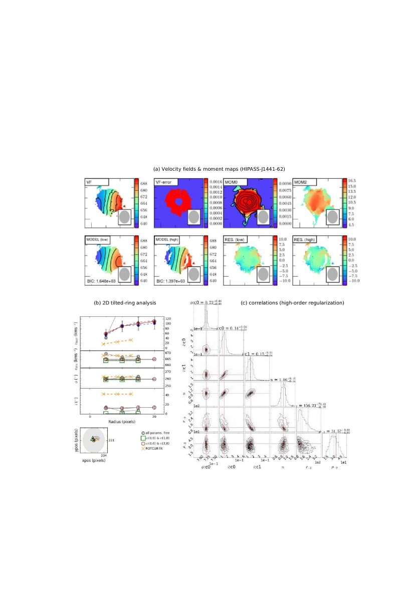
Figure A-2.1.— 2dbat analysis for HIPASS J1441-62: Contours in (a) are spaced by 10 $\mathrm{km}\,\mathrm{s}^{-1}$ on the velocity fields, and 0.1 $\rm mJy\,beam^{-1}$ on the moment 0. The pixel scale in (b) is 5 ″. See Appendix section A.2 for details.

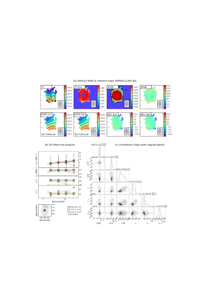
Figure A-2.2.— 2dbat analysis for HIPASS J1305-40: Contours in (a) are spaced by 2 $\mathrm{km}\,\mathrm{s}^{-1}$ on the velocity fields, and 0.1 $\rm mJy\,beam^{-1}$ on the moment 0. The pixel scale in (b) is 4 ″. See Appendix section A.2 for details.

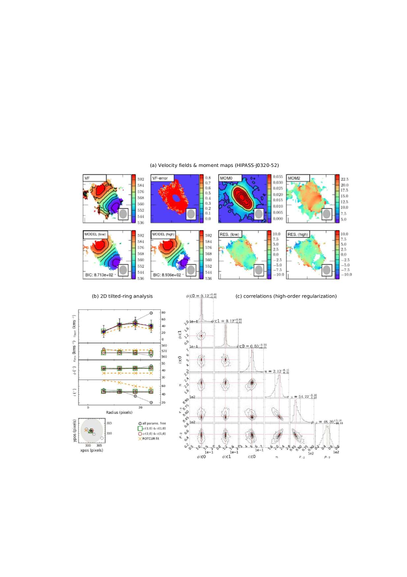
Figure A-2.3.— 2dbat analysis for HIPASS J0320-52: Contours in (a) are spaced by 10 $\mathrm{km}\,\mathrm{s}^{-1}$ on the velocity fields, and 0.1 $\rm mJy\,beam^{-1}$ on the moment 0. The pixel scale in (b) is 5 ″. See Appendix section A.2 for details.

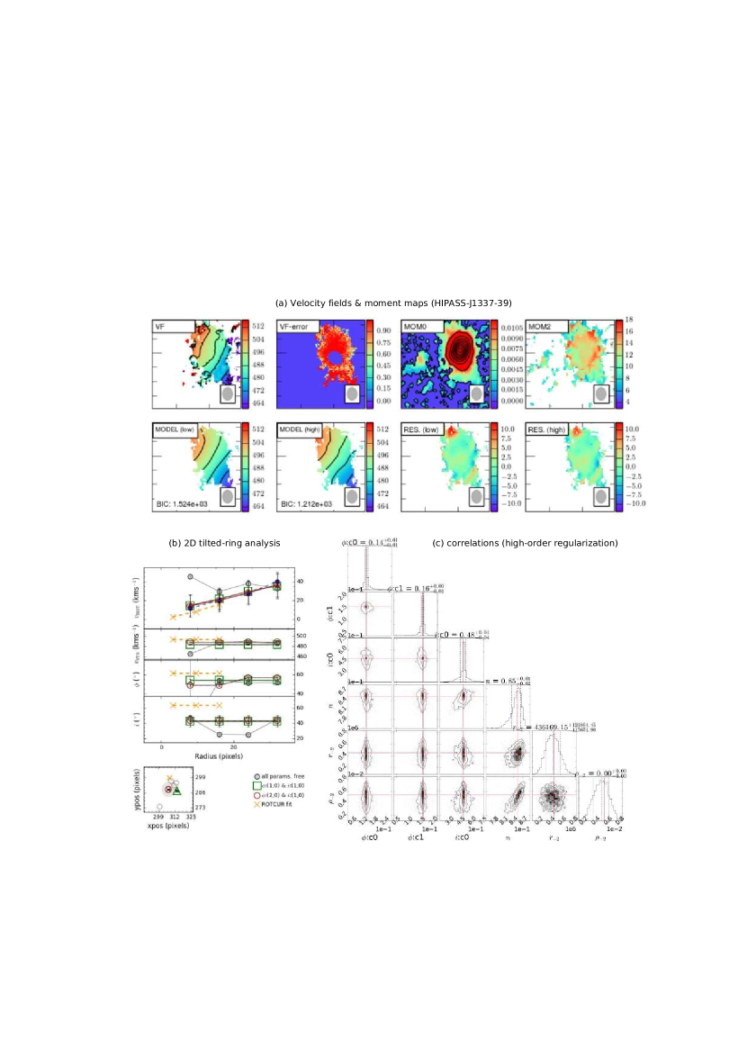
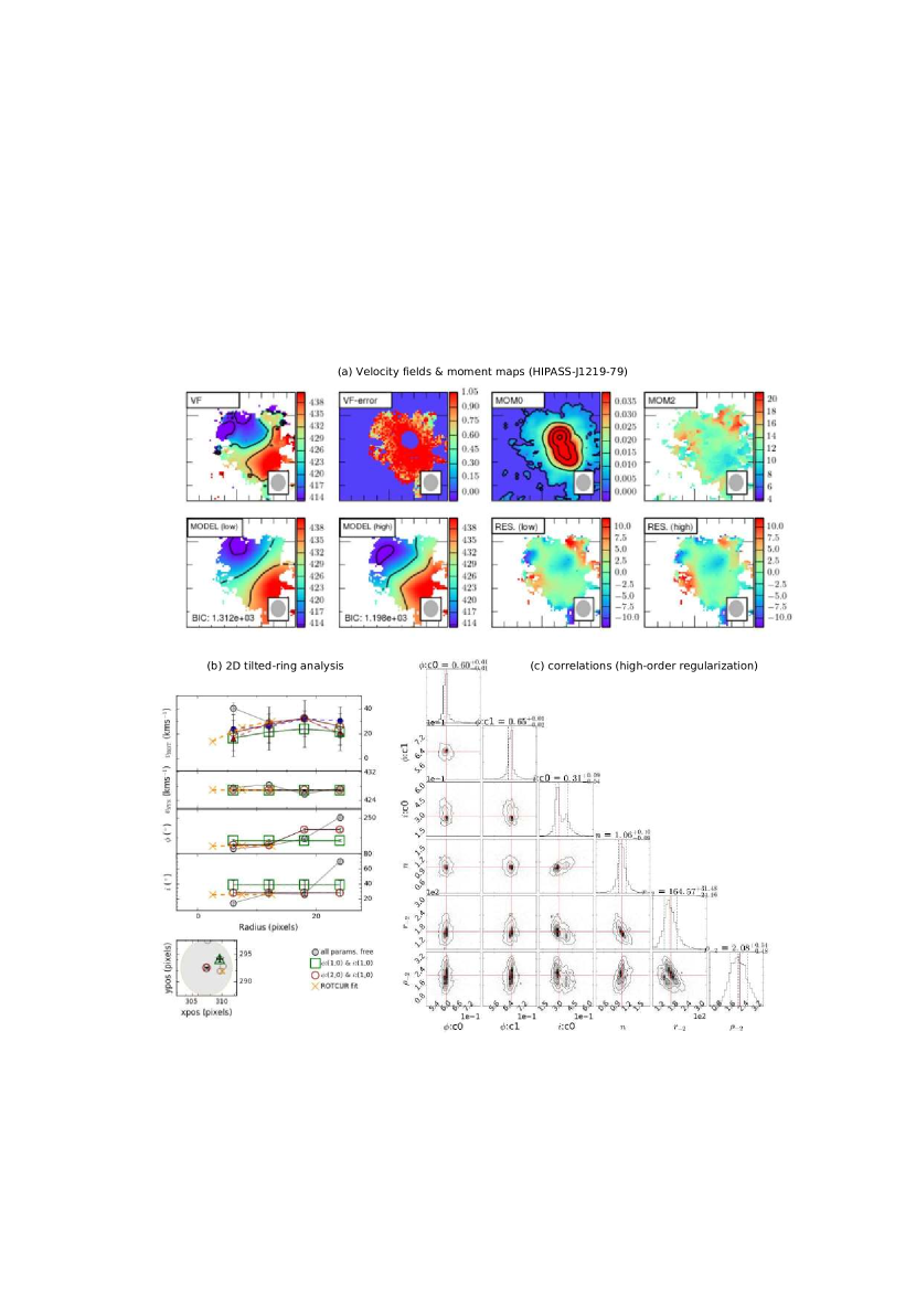
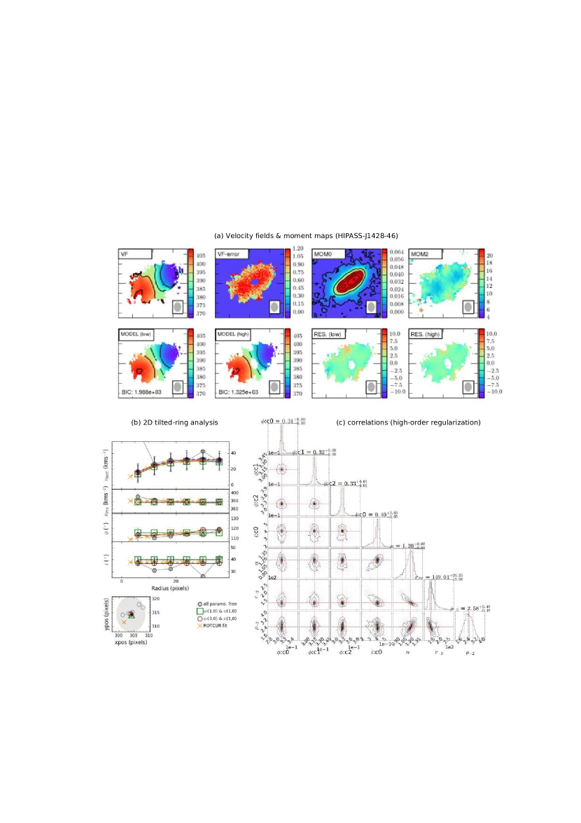
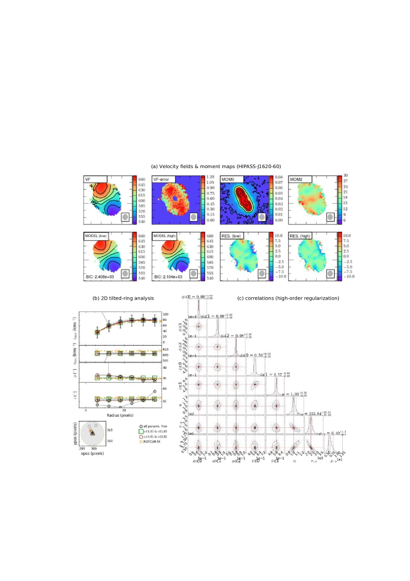
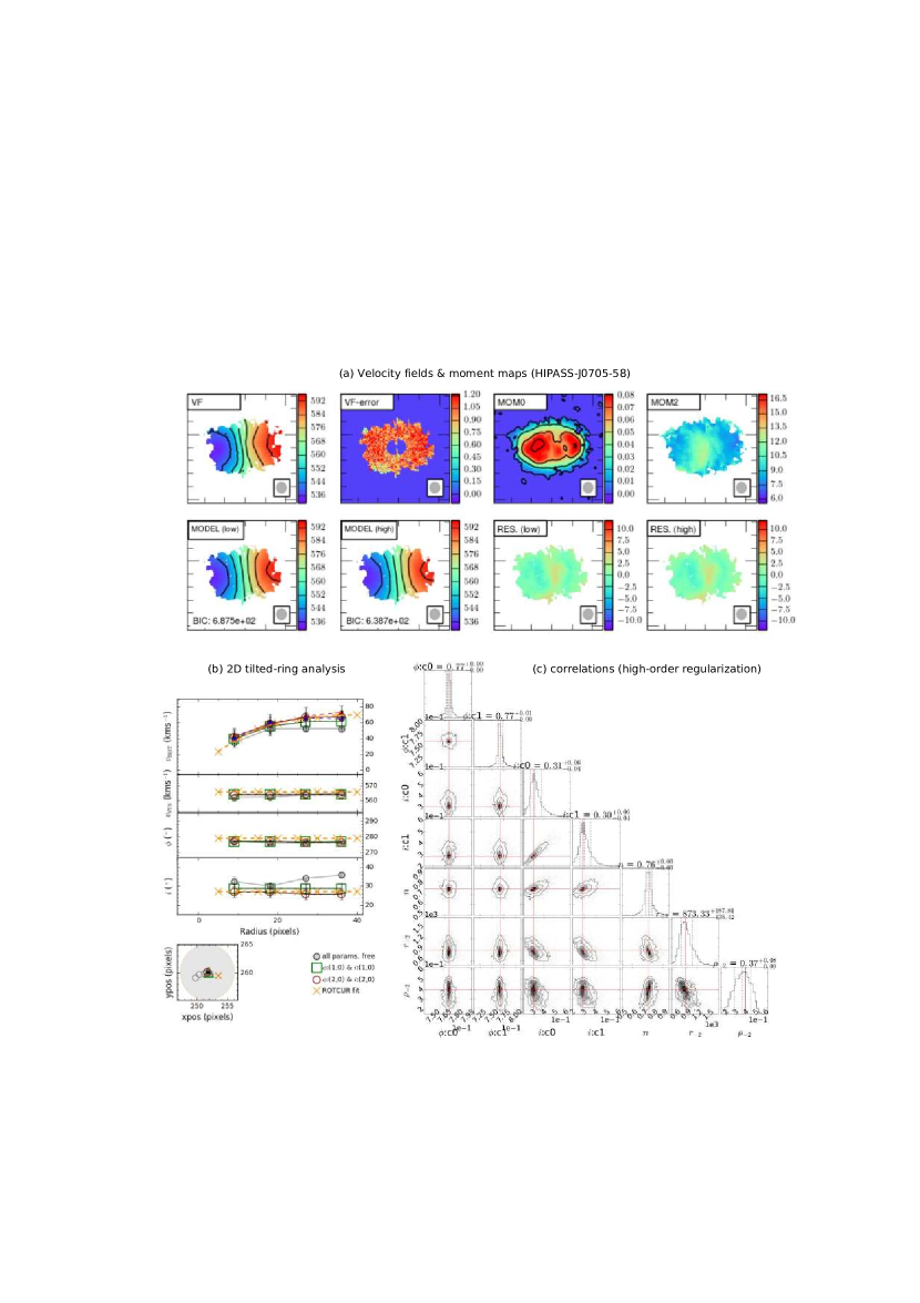
Figure A-2.4.— 2dbat analysis for HIPASS J1337-39: Contours in (a) are spaced by 10 $\mathrm{km}\,\mathrm{s}^{-1}$ on the velocity fields, and 0.1 $\rm mJy\,beam^{-1}$ on the moment 0. The pixel scale in (b) is 5 ″. See Appendix section A.2 for details.

Figure A-2.5.— 2dbat analysis for HIPASS J1219-79: Contours in (a) are spaced by 10 $\mathrm{km}\,\mathrm{s}^{-1}$ on the velocity fields, and 0.1 $\rm mJy\,beam^{-1}$ on the moment 0. The pixel scale in (b) is 5 ″. See Appendix section A.2 for details.

Figure A-2.6.— 2dbat analysis for HIPASS J1047-38: Contours in (a) are spaced by 10 $\mathrm{km}\,\mathrm{s}^{-1}$ on the velocity fields, and 0.1 $\rm mJy\,beam^{-1}$ on the moment 0. The pixel scale in (b) is 5 ″. See Appendix section A.2 for details.

Figure A-2.7.— 2dbat analysis for HIPASS J1428-46: Contours in (a) are spaced by 10 $\mathrm{km}\,\mathrm{s}^{-1}$ on the velocity fields, and 0.1 $\rm mJy\,beam^{-1}$ on the moment 0. The pixel scale in (b) is 5 ″. See Appendix section A.2 for details.

Figure A-2.8.— 2dbat analysis for HIPASS J1620-60: Contours in (a) are spaced by 20 $\mathrm{km}\,\mathrm{s}^{-1}$ on the velocity fields, and 0.1 $\rm mJy\,beam^{-1}$ on the moment 0. The pixel scale in (b) is 5 ″. See Appendix section A.2 for details.

Figure A-2.9.— 2dbat analysis for HIPASS J0705-58: Contours in (a) are spaced by 10 $\mathrm{km}\,\mathrm{s}^{-1}$ on the velocity fields, and 0.1 $\rm mJy\,beam^{-1}$ on the moment 0. The pixel scale in (b) is 6 ″. See Appendix section A.2 for details.

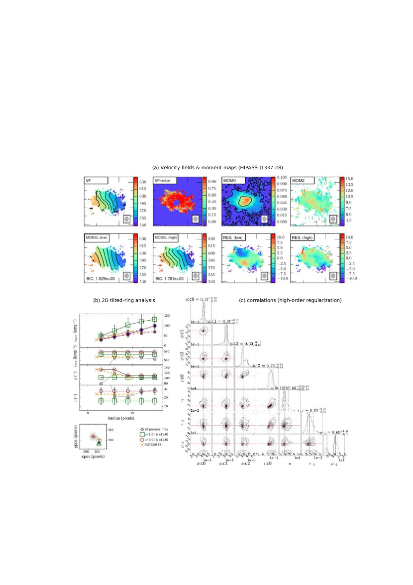
Figure A-2.10.— 2dbat analysis for HIPASS J1337-28: Contours in (a) are spaced by 10 $\mathrm{km}\,\mathrm{s}^{-1}$ on the velocity fields, and 0.1 $\rm mJy\,beam^{-1}$ on the moment 0. The pixel scale in (b) is 5 ″. See Appendix section A.2 for details.

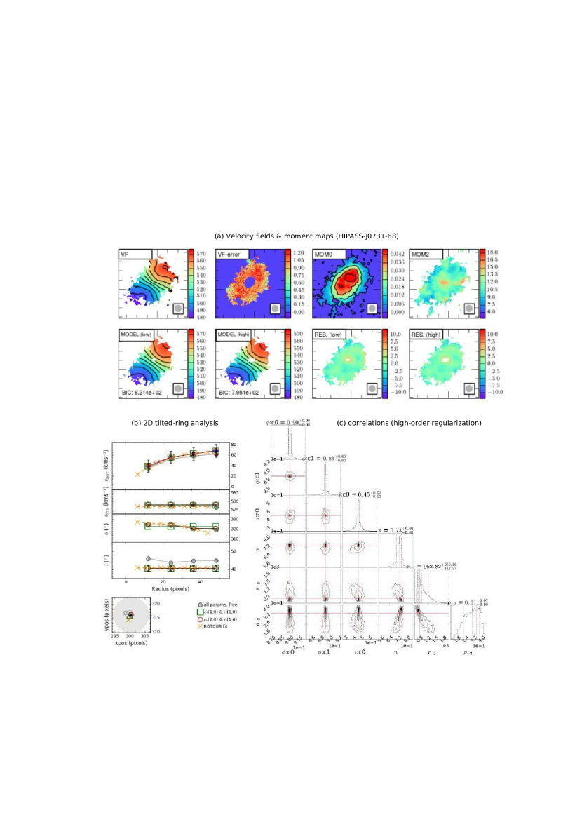
Figure A-2.11.— 2dbat analysis for HIPASS J0731-68: Contours in (a) are spaced by 10 $\mathrm{km}\,\mathrm{s}^{-1}$ on the velocity fields, and 0.1 $\rm mJy\,beam^{-1}$ on the moment 0. The pixel scale in (b) is 4 ″. See Appendix section A.2 for details.

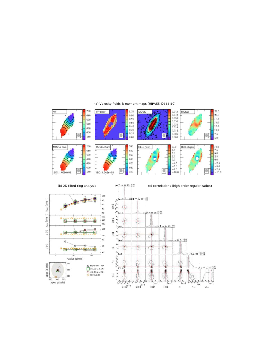
Figure A-2.12.— 2dbat analysis for HIPASS J0333-50: Contours in (a) are spaced by 20 $\mathrm{km}\,\mathrm{s}^{-1}$ on the velocity fields, and 0.1 $\rm mJy\,beam^{-1}$ on the moment 0. The pixel scale in (b) is 5 ″. See Appendix section A.2 for details.

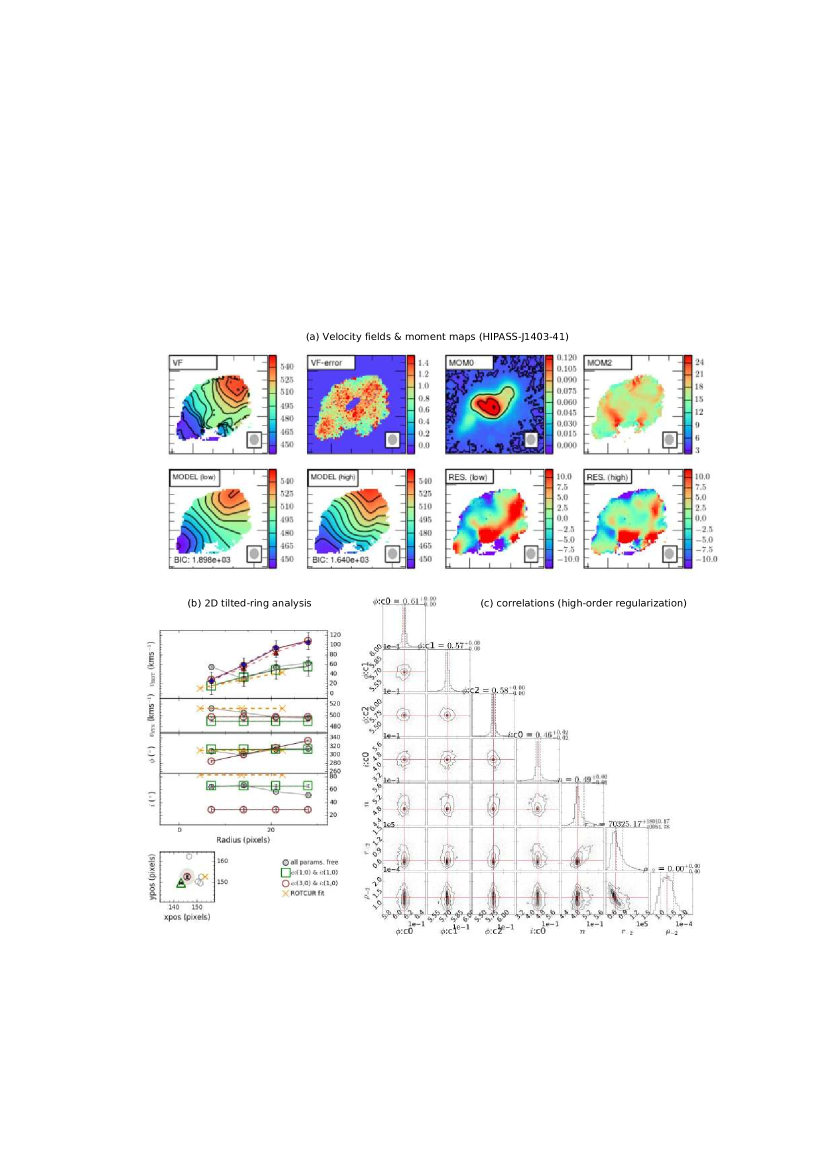
Figure A-2.13.— 2dbat analysis for HIPASS J1403-41: Contours in (a) are spaced by 10 $\mathrm{km}\,\mathrm{s}^{-1}$ on the velocity fields, and 0.1 $\rm mJy\,beam^{-1}$ on the moment 0. The pixel scale in (b) is 10 ″. See Appendix section A.2 for details.

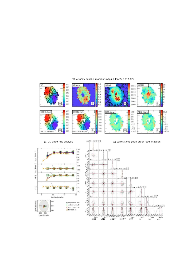
Figure A-2.14.— 2dbat analysis for HIPASS J1337-42: Contours in (a) are spaced by 10 $\mathrm{km}\,\mathrm{s}^{-1}$ on the velocity fields, and 0.1 $\rm mJy\,beam^{-1}$ on the moment 0. The pixel scale in (b) is 4 ″. See Appendix section A.2 for details.

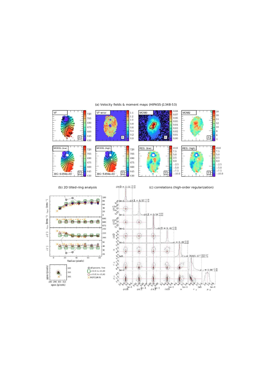
Figure A-2.15.— 2dbat analysis for HIPASS J1348-53: Contours in (a) are spaced by 10 $\mathrm{km}\,\mathrm{s}^{-1}$ on the velocity fields, and 0.1 $\rm mJy\,beam^{-1}$ on the moment 0. The pixel scale in (b) is 5 ″. See Appendix section A.2 for details.

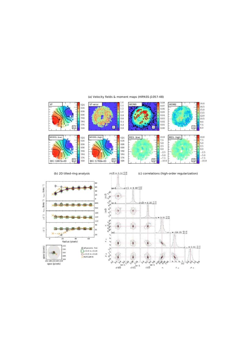
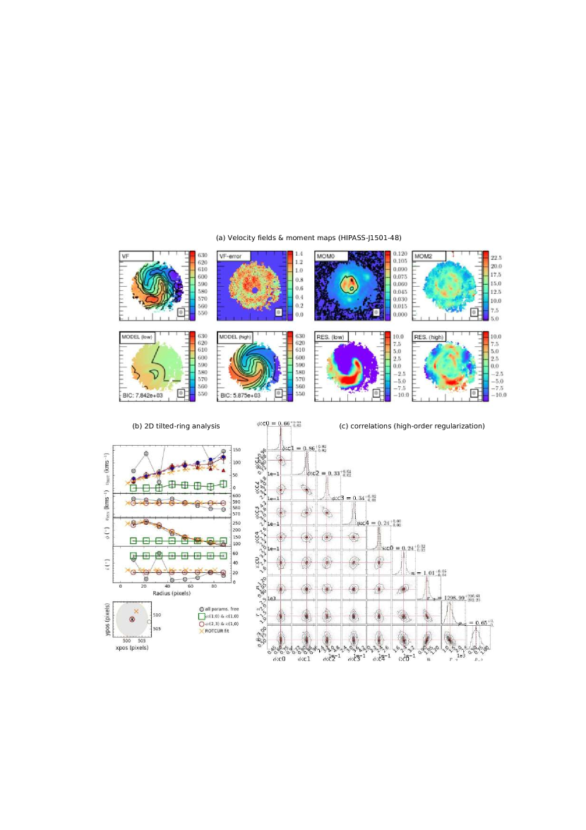
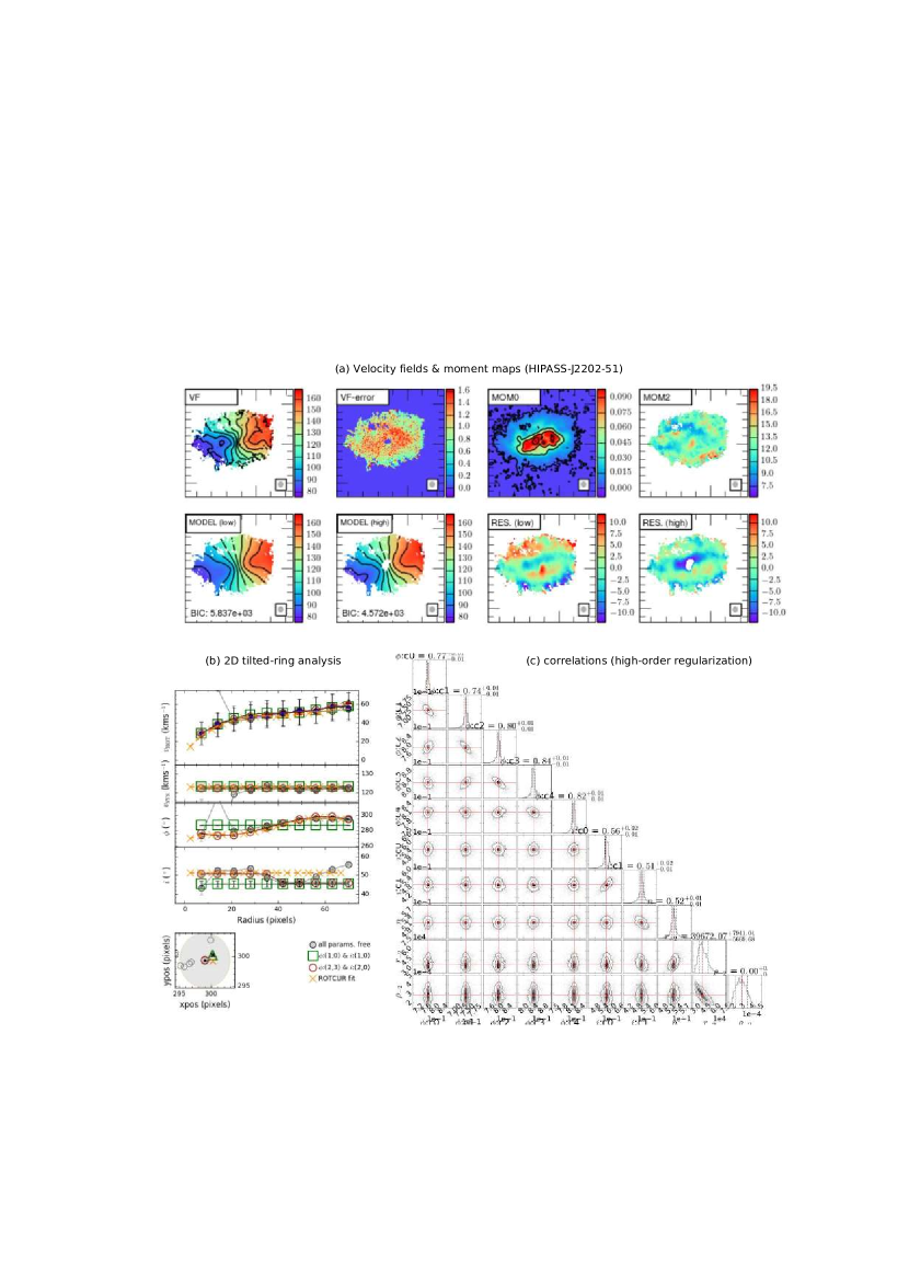
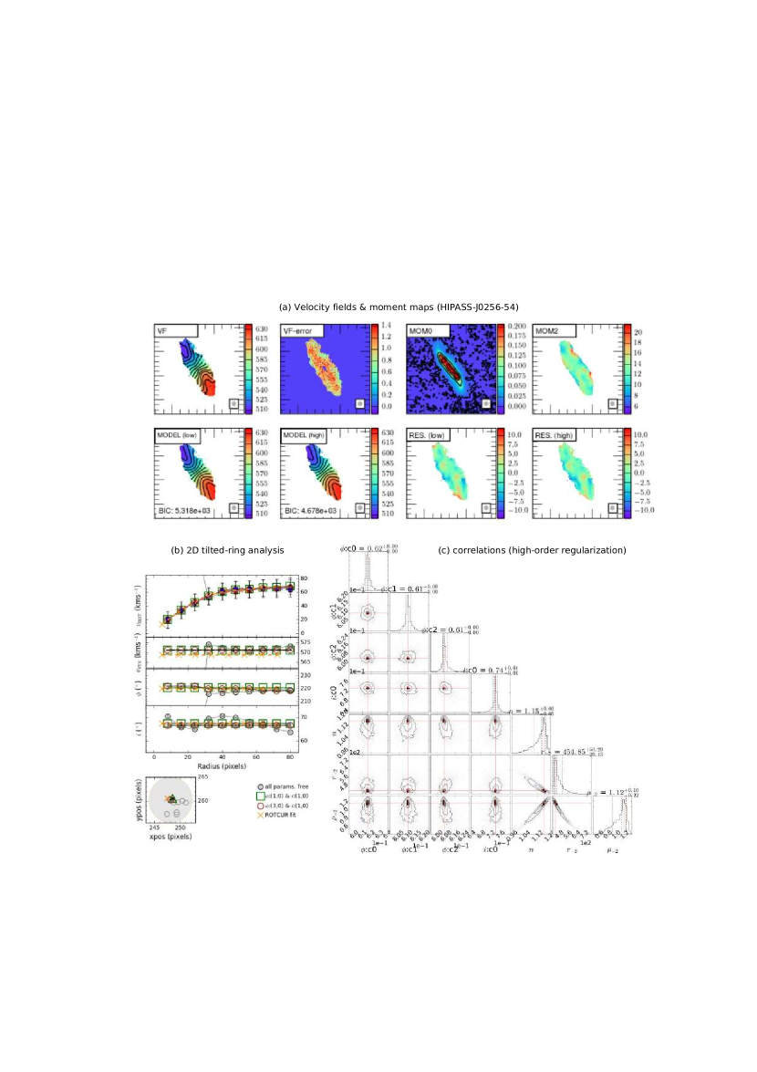
Figure A-2.16.— 2dbat analysis for HIPASS J1057-48: Contours in (a) are spaced by 10 $\mathrm{km}\,\mathrm{s}^{-1}$ on the velocity fields, and 0.1 $\rm mJy\,beam^{-1}$ on the moment 0. The pixel scale in (b) is 5 ″. See Appendix section A.2 for details.

Figure A-2.17.— 2dbat analysis for HIPASS J1501-48: Contours in (a) are spaced by 10 $\mathrm{km}\,\mathrm{s}^{-1}$ on the velocity fields, and 0.1 $\rm mJy\,beam^{-1}$ on the moment 0. The pixel scale in (b) is 5 ″. See Appendix section A.2 for details.

Figure A-2.18.— 2dbat analysis for HIPASS J2202-51: Contours in (a) are spaced by 10 $\mathrm{km}\,\mathrm{s}^{-1}$ on the velocity fields, and 0.1 $\rm mJy\,beam^{-1}$ on the moment 0. The pixel scale in (b) is 5 ″. See Appendix section A.2 for details.

Figure A-2.19.— 2dbat analysis for HIPASS J0256-54: Contours in (a) are spaced by 10 $\mathrm{km}\,\mathrm{s}^{-1}$ on the velocity fields, and 0.1 $\rm mJy\,beam^{-1}$ on the moment 0. The pixel scale in (b) is 6 ″. See Appendix section A.2 for details.

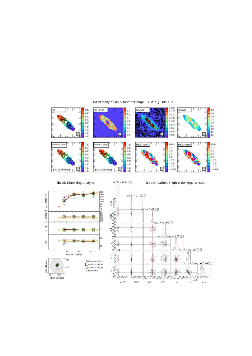
Figure A-2.20.— 2dbat analysis for HIPASS J1305-49: Contours in (a) are spaced by 30 $\mathrm{km}\,\mathrm{s}^{-1}$ on the velocity fields, and 0.1 $\rm mJy\,beam^{-1}$ on the moment 0. The pixel scale in (b) is 10 ″. See Appendix section A.2 for details.

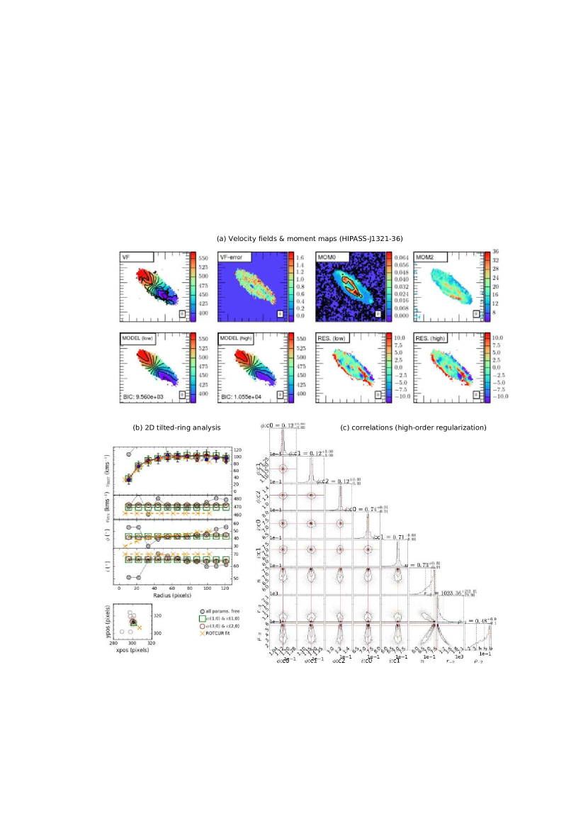
Figure A-2.21.— 2dbat analysis for HIPASS J1321-36: Contours in (a) are spaced by 20 $\mathrm{km}\,\mathrm{s}^{-1}$ on the velocity fields, and 0.1 $\rm mJy\,beam^{-1}$ on the moment 0. The pixel scale in (b) is 5 ″. See Appendix section A.2 for details.

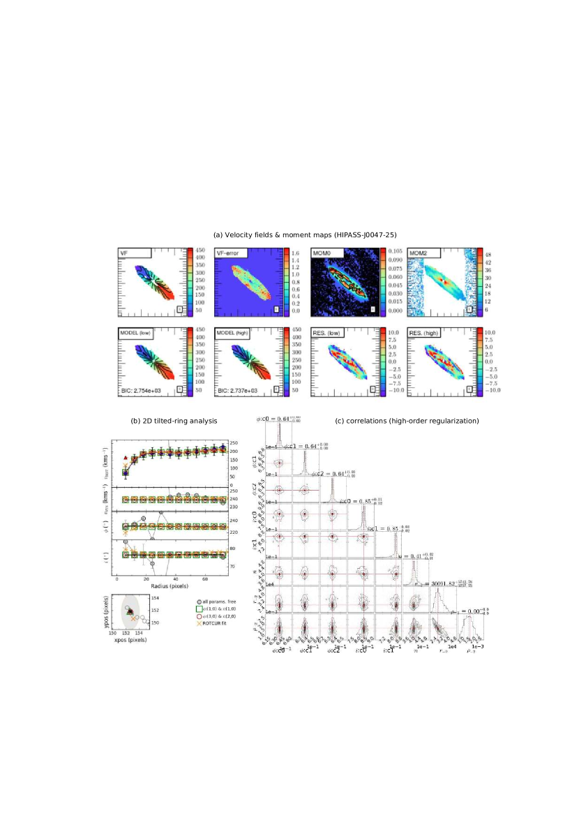
Figure A-2.22.— 2dbat analysis for HIPASS J0047-25: Contours in (a) are spaced by 40 $\mathrm{km}\,\mathrm{s}^{-1}$ on the velocity fields, and 0.1 $\rm mJy\,beam^{-1}$ on the moment 0. The pixel scale in (b) is 10 ″. See Appendix section A.2 for details.

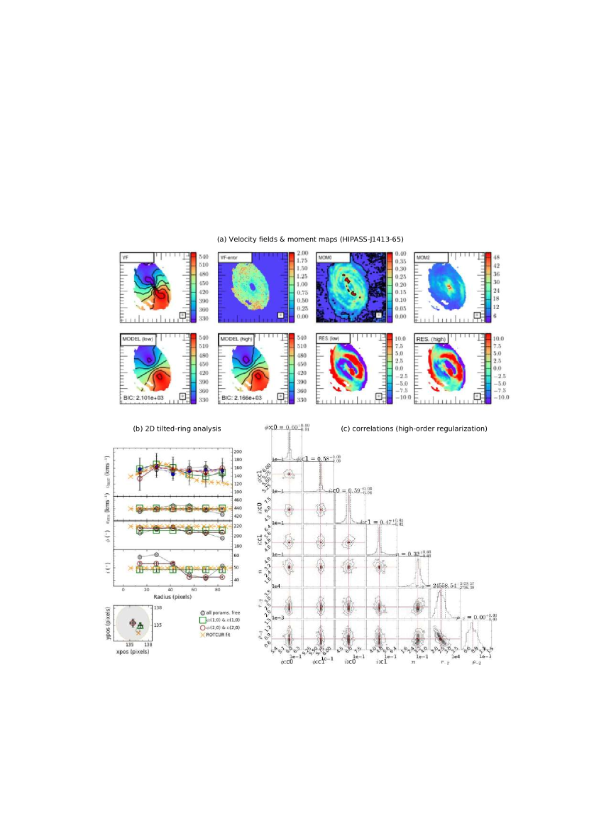
Figure A-2.23.— 2dbat analysis for HIPASS J1413-65: Contours in (a) are spaced by 40 $\mathrm{km}\,\mathrm{s}^{-1}$ on the velocity fields, and 0.1 $\rm mJy\,beam^{-1}$ on the moment 0. The pixel scale in (b) is 20 ″. See Appendix section A.2 for details.

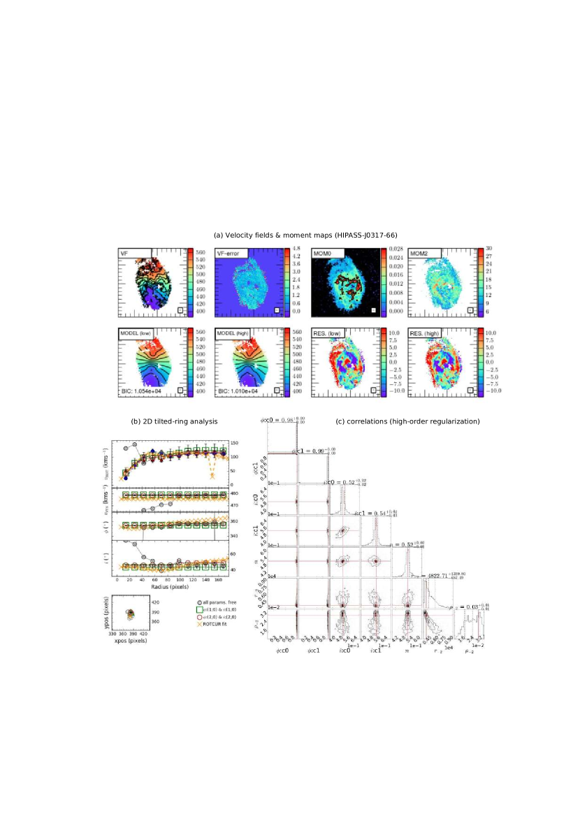
Figure A-2.24.— 2dbat analysis for HIPASS J0317-66: Contours in (a) are spaced by 20 $\mathrm{km}\,\mathrm{s}^{-1}$ on the velocity fields, and 0.1 $\rm mJy\,beam^{-1}$ on the moment 0. The pixel scale in (b) is 2.75 ″. See Appendix section A.2 for details.

References

- Abdussalam et al. (2010) Abdussalam, S. S., Allanach, B. C., Quevedo, F., Feroz, F., & Hobson, M. 2010, Phys. Rev. D, 81, 095012
- Allison et al. (2012) Allison, J. R., Sadler, E. M., & Whiting, M. T. 2012, PASA, 29, 221
- Begeman (1989) Begeman, K. G. 1989, A&A, 223, 47
- Begeman et al. (1991) Begeman, K. G., Broeils, A. H., & Sanders, R. H. 1991, MNRAS, 249, 523
- Begum & Chengalur (2003) Begum, A. & Chengalur, J. N. 2003, A&A, 409, 879
- Begum et al. (2008) Begum, A., Chengalur, J. N., Karachentsev, I. D., Sharina, M. E., & Kaisin, S. S. 2008, MNRAS, 386, 1667
- Borriello & Salucci (2001) Borriello, A. & Salucci, P. 2001, MNRAS, 323, 285
- Bosma (1978) Bosma, A. 1978, PhD thesis, PhD Thesis, Groningen Univ., (1978)
- Bosma (1981a) —. 1981a, AJ, 86, 1791
- Bosma (1981b) —. 1981b, AJ, 86, 1825
- Bouché et al. (2015) Bouché, N., Carfantan, H., Schroetter, I., Michel-Dansac, L., & Contini, T. 2015, AJ, 150, 92
- Broeils & van Woerden (1994) Broeils, A. H. & van Woerden, H. 1994, A&AS, 107, 129
- Cardone et al. (2005) Cardone, V. F., Piedipalumbo, E., & Tortora, C. 2005, MNRAS, 358, 1325
- Carignan (1985) Carignan, C. 1985, ApJ, 299, 59
- Casella & George (1992) Casella, G. & George, E. I. 1992, The American Statistician, 46, 167
- Chemin et al. (2011) Chemin, L., de Blok, W. J. G., & Mamon, G. A. 2011, AJ, 142, 109
- Ciardullo et al. (1993) Ciardullo, R., Jacoby, G. H., & Dejonghe, H. B. 1993, ApJ, 414, 454
- Cormen et al. (2009) Cormen, T. H., Leiserson, C. E., Rivest, R. L., & Stein, C. 2009, Introduction to Algorithms, Third Edition, 3rd edn. (The MIT Press)
- Croom et al. (2012) Croom, S. M., Lawrence, J. S., Bland-Hawthorn, J., Bryant, J. J., Fogarty, L., Richards, S., Goodwin, M., Farrell, T., Miziarski, S., Heald, R., Jones, D. H., Lee, S., Colless, M., Brough, S., Hopkins, A. M., Bauer, A. E., Birchall, M. N., Ellis, S., Horton, A., Leon-Saval, S., Lewis, G., López-Sánchez, Á. R., Min, S.-S., Trinh, C., & Trowland, H. 2012, MNRAS, 421, 872
- Dawid (1973) Dawid, A. P. 1973, Biometrika, 60, 664
- de Blok & McGaugh (1997) de Blok, W. J. G. & McGaugh, S. S. 1997, MNRAS, 290, 533
- de Blok et al. (2008) de Blok, W. J. G., Walter, F., Brinks, E., Trachternach, C., Oh, S.-H., & Kennicutt, Jr., R. C. 2008, AJ, 136, 2648
- de Boor (1978) de Boor, C. 1978, A practical guide to splines
- Di Teodoro & Fraternali (2015) Di Teodoro, E. M. & Fraternali, F. 2015, MNRAS, 451, 3021
- Duffy et al. (2012) Duffy, A. R., Meyer, M. J., Staveley-Smith, L., Bernyk, M., Croton, D. J., Koribalski, B. S., Gerstmann, D., & Westerlund, S. 2012, MNRAS, 426, 3385
- Einasto (1965) Einasto, J. 1965, Trudy Astrofizicheskogo Instituta Alma-Ata, 5, 87
- Einasto (1968) —. 1968, Publications of the Tartu Astrofizica Observatory, 36, 414
- Feroz et al. (2011) Feroz, F., Balan, S. T., & Hobson, M. P. 2011, MNRAS, 415, 3462
- Feroz et al. (2009a) Feroz, F., Gair, J. R., Hobson, M. P., & Porter, E. K. 2009a, Classical and Quantum Gravity, 26, 215003
- Feroz & Hobson (2008) Feroz, F. & Hobson, M. P. 2008, MNRAS, 384, 449
- Feroz et al. (2009b) Feroz, F., Hobson, M. P., & Bridges, M. 2009b, MNRAS, 398, 1601
- Feroz et al. (2013) Feroz, F., Hobson, M. P., Cameron, E., & Pettitt, A. N. 2013, ArXiv e-prints
- Geman & Geman (1984) Geman, S. & Geman, D. 1984, IEEE Trans. Pattern Anal. Mach. Intell., 6, 721 [LINK]
- Gentile et al. (2010) Gentile, G., Baes, M., Famaey, B., & van Acoleyen, K. 2010, MNRAS, 406, 2493
- Hastings (1970) Hastings, W. K. 1970, BIOMETRIKA, 57, 97
- Heald et al. (2011) Heald, G., Józsa, G., Serra, P., Zschaechner, L., Rand, R., Fraternali, F., Oosterloo, T., Walterbos, R., Jütte, E., & Gentile, G. 2011, A&A, 526, A118
- Herrmann (2008) Herrmann, K. A. 2008, PhD thesis, The Pennsylvania State University
- Hron (1987) Hron, J. 1987, A&A, 176, 34
- Huchtmeier et al. (1981) Huchtmeier, W. K., Seiradakis, J. H., & Materne, J. 1981, A&A, 102, 134
- Hunter et al. (2012) Hunter, D. A., Ficut-Vicas, D., Ashley, T., Brinks, E., Cigan, P., Elmegreen, B. G., Heesen, V., Herrmann, K. A., Johnson, M., Oh, S.-H., Rupen, M. P., Schruba, A., Simpson, C. E., Walter, F., Westpfahl, D. J., Young, L. M., & Zhang, H.-X. 2012, AJ, 144, 134
- Johnston et al. (2008) Johnston, S., Taylor, R., Bailes, M., Bartel, N., Baugh, C., Bietenholz, M., Blake, C., Braun, R., Brown, J., Chatterjee, S., Darling, J., Deller, A., Dodson, R., Edwards, P., Ekers, R., Ellingsen, S., Feain, I., Gaensler, B., Haverkorn, M., Hobbs, G., Hopkins, A., Jackson, C., James, C., Joncas, G., Kaspi, V., Kilborn, V., Koribalski, B., Kothes, R., Landecker, T., Lenc, E., Lovell, J., Macquart, J.-P., Manchester, R., Matthews, D., McClure-Griffiths, N., Norris, R., Pen, U.-L., Phillips, C., Power, C., Protheroe, R., Sadler, E., Schmidt, B., Stairs, I., Staveley-Smith, L., Stil, J., Tingay, S., Tzioumis, A., Walker, M., Wall, J., & Wolleben, M. 2008, Experimental Astronomy, 22, 151
- Józsa et al. (2007) Józsa, G. I. G., Kenn, F., Klein, U., & Oosterloo, T. A. 2007, A&A, 468, 731
- Kamphuis et al. (2015) Kamphuis, P., Józsa, G. I. G., Oh, S.-. H., Spekkens, K., Urbancic, N., Serra, P., Koribalski, B. S., & Dettmar, R.-J. 2015, MNRAS, 452, 3139
- Kamphuis et al. (2013) Kamphuis, P., Rand, R. J., Józsa, G. I. G., Zschaechner, L. K., Heald, G. H., Patterson, M. T., Gentile, G., Walterbos, R. A. M., Serra, P., & de Blok, W. J. G. 2013, MNRAS, 434, 2069
- Koribalski (2010) Koribalski, B. S. 2010, in Astronomical Society of the Pacific Conference Series, Vol. 421, Galaxies in Isolation: Exploring Nature Versus Nurture, ed. L. Verdes-Montenegro, A. Del Olmo, & J. Sulentic, 137
- Koribalski (2012) Koribalski, B. S. 2012, PASA, 29, 359
- Koribalski et al. (2004) Koribalski, B. S., Staveley-Smith, L., Kilborn, V. A., Ryder, S. D., Kraan-Korteweg, R. C., Ryan-Weber, E. V., Ekers, R. D., Jerjen, H., Henning, P. A., Putman, M. E., Zwaan, M. A., de Blok, W. J. G., Calabretta, M. R., Disney, M. J., Minchin, R. F., Bhathal, R., Boyce, P. J., Drinkwater, M. J., Freeman, K. C., Gibson, B. K., Green, A. J., Haynes, R. F., Juraszek, S., Kesteven, M. J., Knezek, P. M., Mader, S., Marquarding, M., Meyer, M., Mould, J. R., Oosterloo, T., O’Brien, J., Price, R. M., Sadler, E. M., Schröder, A., Stewart, I. M., Stootman, F., Waugh, M., Warren, B. E., Webster, R. L., & Wright, A. E. 2004, AJ, 128, 16
- Krajnović et al. (2006) Krajnović, D., Cappellari, M., de Zeeuw, P. T., & Copin, Y. 2006, MNRAS, 366, 787
- Mamon & Łokas (2005) Mamon, G. A. & Łokas, E. L. 2005, MNRAS, 362, 95
- Martimbeau et al. (1994) Martimbeau, N., Carignan, C., & Roy, J.-R. 1994, AJ, 107, 543
- McGaugh et al. (2001) McGaugh, S. S., Rubin, V. C., & de Blok, W. J. G. 2001, AJ, 122, 2381
- Metropolis et al. (1953) Metropolis, N., Rosenbluth, A., Rosenbluth, M., Teller, A., & Teller, E. 1953, J. Chem. Phys., 21, 1087
- Navarro et al. (1996) Navarro, J. F., Frenk, C. S., & White, S. D. M. 1996, ApJ, 462, 563
- Navarro et al. (2004) Navarro, J. F., Hayashi, E., Power, C., Jenkins, A. R., Frenk, C. S., White, S. D. M., Springel, V., Stadel, J., & Quinn, T. R. 2004, MNRAS, 349, 1039
- Navarro et al. (2010) Navarro, J. F., Ludlow, A., Springel, V., Wang, J., Vogelsberger, M., White, S. D. M., Jenkins, A., Frenk, C. S., & Helmi, A. 2010, MNRAS, 402, 21
- Oh (2009) Oh, S.-H. 2009, PhD thesis, The Australian National University
- Oh et al. (2011) Oh, S.-H., de Blok, W. J. G., Brinks, E., Walter, F., & Kennicutt, Jr., R. C. 2011, AJ, 141, 193
- Ott et al. (2012) Ott, J., Stilp, A. M., Warren, S. R., Skillman, E. D., Dalcanton, J. J., Walter, F., de Blok, W. J. G., Koribalski, B., & West, A. A. 2012, AJ, 144, 123
- Pence (1999) Pence, W. Astronomical Society of the Pacific Conference Series, Vol. 172, , Astronomical Data Analysis Software and Systems VIII, ed. D. M. MehringerR. L. Plante & D. A. Roberts, 487
- Peters et al. (2017) Peters, S. P. C., van der Kruit, P. C., Allen, R. J., & Freeman, K. C. 2017, MNRAS, 464, 21
- Press et al. (1992) Press, W. H., Flannery, B. P., Teukolsky, S. A., & Vetterling, W. T. 1992 (Numerical Recipes in Fortran: The Art of Scientific Computing)
- Rogstad et al. (1974) Rogstad, D. H., Lockhart, I. A., & Wright, M. C. H. 1974, ApJ, 193, 309
- Rubin et al. (1980) Rubin, V. C., Ford, W. K. J., & . Thonnard, N. 1980, ApJ, 238, 471
- Schinnerer et al. (2000) Schinnerer, E., Eckart, A., Tacconi, L. J., Genzel, R., & Downes, D. 2000, ApJ, 533, 850
- Sellwood & Sánchez (2010) Sellwood, J. A. & Sánchez, R. Z. 2010, MNRAS, 404, 1733
- Serra et al. (2015) Serra, P., Koribalski, B., Kilborn, V., Allison, J. R., Amy, S. W., Ball, L., Bannister, K., Bell, M. E., Bock, D. C.-J., Bolton, R., Bowen, M., Boyle, B., Broadhurst, S., Brodrick, D., Brothers, M., Bunton, J. D., Chapman, J., Cheng, W., Chippendale, A. P., Chung, Y., Cooray, F., Cornwell, T., DeBoer, D., Diamond, P., Forsyth, R., Gough, R., Gupta, N., Hampson, G. A., Harvey-Smith, L., Hay, S., Hayman, D. B., Heywood, I., Hotan, A. W., Hoyle, S., Humphreys, B., Indermuehle, B., Jacka, C., Jackson, C. A., Jackson, S., Jeganathan, K., Johnston, S., Joseph, J., Kamphuis, P., Leach, M., Lenc, E., Lensson, E., Mackay, S., Marquarding, M., Marvil, J., McClure-Griffiths, N., McConnell, D., Meyer, M., Mirtschin, P., Neuhold, S., Ng, A., Norris, R. P., O’Sullivan, J., Pathikulangara, J., Pearce, S., Phillips, C., Popping, A., Qiao, R. Y., Reynolds, J. E., Roberts, P., Sault, R. J., Schinckel, A. E. T., Shaw, R., Shimwell, T. W., Staveley-Smith, L., Storey, M., Sweetnam, A. W., Troup, E., Tzioumis, A., Voronkov, M. A., Westmeier, T., Whiting, M., Wilson, C., Wong, O. I., & Wu, X. 2015, MNRAS, 452, 2680
- Sivia (2006) Sivia, D. 2006 (Data Analysis-A Baysian Tutorial (Oxford University Press, Oxford))
- Sivia & Skilling (2006) Sivia, D. & Skilling, J. 2006, Data analysis: a Bayesian tutorial, Oxford science publications (Oxford University Press) [LINK]
- Skilling (2004) Skilling, J. American Institute of Physics Conference Series, ed. , R. FischerR. Preuss & U. V. Toussaint, 395–405 [LINK]
- Sofue & Rubin (2001) Sofue, Y. & Rubin, V. 2001, ARA&A, 39, 137
- Spekkens & Sellwood (2007) Spekkens, K. & Sellwood, J. A. 2007, ApJ, 664, 204
- Swaters (1999) Swaters, R. A. 1999 (PhD Thesis, University of Groningen)
- Teuben (2002) Teuben, P. J. Astronomical Society of the Pacific Conference Series, Vol. 275, , Disks of Galaxies: Kinematics, Dynamics and Peturbations, ed. E. AthanassoulaA. Bosma & R. Mujica, 217–228
- Tully & Fisher (1977) Tully, R. B. & Fisher, J. R. 1977, A&A, 54, 661
- van der Hulst (2002) van der Hulst, J. M. Astronomical Society of the Pacific Conference Series, Vol. 276, , Seeing Through the Dust: The Detection of HI and the Exploration of the ISM in Galaxies, ed. A. R. TaylorT. L. Landecker & A. G. Willis, 84
- Walter et al. (2008) Walter, F., Brinks, E., de Blok, W. J. G., Bigiel, F., Kennicutt, Jr., R. C., Thornley, M. D., & Leroy, A. 2008, AJ, 136, 2563
- Wang et al. (2016) Wang, J., Koribalski, B. S., Serra, P., van der Hulst, T., Roychowdhury, S., Kamphuis, P., & Chengalur, J. N. 2016, MNRAS, 460, 2143
- Weldrake et al. (2003) Weldrake, D. T. F., de Blok, W. J. G., & Walter, F. 2003, MNRAS, 340, 12
- Wong et al. (2004) Wong, T., Blitz, L., & Bosma, A. 2004, ApJ, 605, 183
- Wright (1974) Wright, M. C. H. G. L. Verschuur, K. I. Kellermann & V. van Brunt, 291
- Zschaechner et al. (2011) Zschaechner, L. K., Rand, R. J., Heald, G. H., Gentile, G., & Kamphuis, P. 2011, ApJ, 740, 35