Chaos in Saw Map

Abstract

We consider dynamics of a scalar piecewise linear ”saw map” with infinitely many linear segments. In particular, such maps are generated as a Poincaré map of simple two-dimensional discrete time piecewise linear systems involving a saturation function. Alternatively, these systems can be viewed as a feedback loop with the so-called stop hysteresis operator. We analyze chaotic sets and attractors of the ”saw map” depending on its parameters.

1 Introduction

Piecewise linear (PWL) and piecewise smooth (PWS) systems serve as a modeling framework for applications involving friction, collision, sliding, intermittently constrained systems and processes with switching components. Examples include stick-slip motion in mechanical systems, impact oscillators, switching electronic circuits (such as DC/DC power converters and relay controllers), hybrid dynamics in control systems as well as models of economics and finance [29, 5]. Low-dimensional nonsmooth maps can also appear as Poincaré return maps of smooth flows which show chaotic dynamics [14, 20].

Since the second half of the 1990s, multiple analytic tools have been developed in order to address distinctive scenarios, which are not observed in smooth dynamical systems but are unique to piecewise smooth systems [9, 26, 17]. For example, these scenarios include robust chaos [4]; various types of discontinuity-induced bifurcations (related to sliding, chattering, grazing and corner collision phenomena) which occur when an invariant set collides with a switching surface; and, border-collision bifurcations of the associated Poincaré maps with their normal forms [24, 21, 22, 12, 28].

One-dimensional maps serve as important prototype models, which help understand dynamics of higher-dimensional systems. Further, one-dimensional dynamics has developed into a subject in its own right [7]. In particular, bifurcation scenarios and symbolic dynamics specific to PWS and PWL maps have been intensively explored in the last two decades [3]. However, they are still understood to a lesser extent than dynamics of smooth maps, and the PWS theory is far from being complete. Even the skew tent map, which is a simple variation of the classical tent map, produces a rich variety of dynamical scenarios which have not been completely described yet (see survey [27] for the state-of-the-art results).

In this paper, we consider dynamics of a one-dimensional PWL map, which has infinitely many local maximum and minimum points accumulating near an essential discontinuity point, see Fig. 1. We call it a “saw map”. As a matter of fact, this map represents a reduction of a two-dimensional PWL map including a linear term and the simple saturation PWL function (see (15) below) to a one-dimensional Poincaré map [2]. The objective of this work is to analyze chaotic repelling and attracting sets, including robust chaos, for a general class of such one-dimensional maps. The “saw map” can have multiple attractors embedded into a number of invariant intervals. One of such intervals contains infinitely many local maximum and minimum points of the map, while the restriction of the map to any other invariant interval is a skew tent map. The paper is organized as follows. In the main Section 2, we consider dynamics of the “saw map” depending on its parameters. In particular, we obtain a characterization of the attractor of the skew tent map, which to the best of our knowledge is new (see Remark 2 to formula (5) of Theorem 2.2). In Section 3, we discuss the implications of our results for the 2-dimensional PWL map with the saturation nonlinearity. This map has been related to a set of macroeconomic models with sticky inflation and to discrete time systems with dry friction in [2].

2 Main results

There are several definitions of a chaotic invariant set. We use the definition of R. Devaney [8].

A closed invariant set $A$ for the map $f$ is chaotic if:

• (density of periodic orbits) periodic points of $f$ are dense in $A$;

• (sensitivity to initial conditions) there is a $\beta>0$ such that for any $x\in A$ and any $\epsilon>0$ there is a $y\in A$ with $|x-y|<\epsilon$ and a $k$ such that $|f^{k}(x)-f^{k}(y)|>\beta$;

• (topological mixing or transitivity) $A$ contains a dense orbit of $f$.

In what follows, we use the notation $A\subset B$ if $A\subseteq B$, $A\neq B$. By $\overline{A}$ we denote the closure of a set $A$.

By $|I|$ we denote the length of an interval $I$.

Let sequences $p_{k},q_{k},r_{k}$ satisfy

$$\begin{array}[]{ll}r_{0}>q_{1}>r_{1}>q_{2}>r_{2}>\cdots>0,&\quad q_{k},r_{k}\to 0,\\ p_{0}>p_{1}>p_{2}>p_{3}>\cdots>0,&\quad p_{0}<r_{0},\quad p_{k}>r_{k}\ \ {\rm for\ all}\ \ k\geq 1.\end{array}$$ (1)

Denote $J=[0,r_{0}]$ and consider a “saw map” $T:J\to\mathbb{R}$ defined by the following properties:

• $T(0)=T(q_{k})=0$ for all $k\geq 1$;

• $T(r_{k})=p_{k}$ for all $k\geq 0$;

• $T$ is linear on each of the intervals $[q_{k+1},r_{k}]$, $[r_{k},q_{k}]$, $k\geq 1$, and $[q_{1},r_{0}]$,

see Fig. 1. These properties and the fact that $p_{0}<r_{0}$ imply that $T(J)\subset J$. Also these properties imply that $T$ has a unique fixed point $e_{k}$ in each interval $(q_{k+1},r_{k})$, $k\geq 1$ and a unique fixed point $\hat{e}_{k}$ in each interval $(r_{k},q_{k})$, $k\geq 1$.

Note that $T$ is piecewise linear and continuous on every segment $[a,b]\subset J\setminus\{0\}$. If $p_{*}:=\lim_{k\to\infty}p_{k}=0$, then $T$ is continuous on $J$. On the other hand, if $p_{*}>0$, then $T$ has a discontinuity at zero. Denote by

$$\alpha_{k}:=p_{k}/(r_{k}-q_{k+1}),\qquad\beta_{k}:=p_{k}/(q_{k}-r_{k})$$

the absolute value of the slope of the graph of $T$ on the intervals $[q_{k+1},r_{k}]$ and $[r_{k},q_{k}]$, respectively. The assumption $p_{k}>r_{k}$, $k\geq 1$ implies that

$$\alpha_{k}>1\quad{\rm for\ all}\quad k\geq 1.$$

We assume additionally that

• $\alpha_{k}$ and $\beta_{k}$ are increasing sequences;

• there exists $k^{*}\geq 1$ such that $p_{k}>e_{k-1}$ for $k\geq k^{*}+1$ and if $k_{*}\geq 2$ then $p_{k}<e_{k-1}$ for $2\leq k\leq k^{*}$;

• for $1\leq k\leq k^{*}-1$,

  $$q_{k}+\frac{e_{k}}{\alpha_{k-1}}>p_{k}.$$ (2)

[width=]saw_pic

Figure 1: Graph of the map $T$.

The last condition is technical. It allows us to simplify the results by shortening the list of possible dynamical scenarios, which are, however, similar to each other.

From the definition of $k^{*}$ it follows that the segment

$$J^{*}=[0,p_{k^{*}}]\subset J$$

is invariant for $T$. A proof of this fact is given in the next section. Consider also the segments

$$J_{k}=[e_{k},p_{k}],\qquad G_{k}=[T^{2}(r_{k}),T(r_{k})]=[T(p_{k}),p_{k}],\quad 1\leq k\leq k^{*},$$ (3)

see Fig. 1. These segments are well-defined. Indeed, $e_{k}<r_{k}<p_{k}$, $k\geq 1$ by definition of $T$. Also, since $p_{k}<e_{k-1}$ for $2\leq k\leq k^{*}$ and $r_{0}>p_{0}$, for $1\leq k\leq k^{*}$ we have $p_{k}>T(p_{k})$.

Remark 1.

Denote

$$f_{k}=\min\{x>e_{k}:\ T(x)=e_{k}\},\qquad 1\leq k\leq k^{*}.$$ (4)

It is easy to see that if $\alpha_{k}^{-1}+\beta_{k}^{-1}\geq 1$, then $f_{k}\geq p_{k}$ and the segment $J_{k}$ is invariant, while if $\alpha_{k}^{-1}+\beta_{k}^{-1}<1$, then $f_{k}<p_{k}$ and the segment $J_{k}$ is not invariant.

Theorem 2.1.

If $\alpha_{k^{*}}^{-1}+\beta_{k^{*}}^{-1}<1$, then the segment $J^{*}$ is a chaotic invariant set. If $\alpha_{k^{*}}^{-1}+\beta_{k^{*}}^{-1}\geq 1$, then the segment $J^{*}$ contains a chaotic invariant Cantor set $\Sigma$. Furthermore, all trajectories from $J^{*}\backslash\Sigma$ reach the invariant segment $J_{k^{*}}\subset J^{*}$ after a finite number of iterations.

In the case $\alpha_{k^{*}}^{-1}+\beta_{k^{*}}^{-1}\geq 1$, dynamics on the invariant interval $J_{k^{*}}$ is described in the next theorem.

Theorem 2.2.

If $\beta_{k}<1$ for some $k\leq k^{*}$ (see Fig. 2(a)), then the interval $J_{k}$ is invariant and $J_{k}\setminus\{e_{k}\}$ belongs to the basin of attraction of the stable fixed point $\hat{e}_{k}\in J_{k}$.

If $\beta_{k}>1$ and $\alpha_{k}^{-1}+\beta_{k}^{-1}>1$ for some $k\leq k^{*}$ (see Fig. 2(b)), then the interval $J_{k}$ is also invariant. Further, the interval $G_{k}\subset J_{k}$ defined in (3) is invariant and contains a chaotic invariant set

$$\Lambda_{k}=\bigcup_{i=1}^{2^{N}}\overline{A_{i}},$$ (5)

where the $A_{i}$ are non-intersecting open intervals. The complement $G_{k}\setminus\Lambda_{k}$ contains $N$ unstable periodic orbits $O_{i}$ of periods $1,\ldots,2^{N-1}$. Furthermore, for any $x\in G_{k}\setminus(\Lambda_{k}\cup O_{1}\cup\cdots\cup O_{N})$ there is an $n_{0}$ such that $T^{n}(x)\in\Lambda_{k}$ for $n\geq n_{0}$, and for any $y\in J_{k}\setminus(G_{k}\cup\{e_{k}\})$ there is an $n_{1}$ such that $T^{n}(y)\in G_{k}$ for $n\geq n_{1}$.

Finally, if $\alpha_{k}^{-1}+\beta_{k}^{-1}<1$ for some $1\leq k\leq k^{*}-1$ (see Fig. 2(c)), then the interval $J_{k}$ contains a chaotic invariant Cantor set $\Lambda_{k}$, dynamics on this set is conjugate to the left shift, and for every $x\in J_{k}\setminus\Lambda_{k}$ there is an $n_{2}$ such that $T^{n}(x)\in[0,e_{k})$ for $n\geq n_{2}$.

[width=0.32]type1

(a)

[width=0.32]type2

(b)

[width=0.32]type3

(c)

Figure 2: Possible shapes of the graph of the map $T$ on an interval $J_{k}$. (a) $\beta_{k}<1$; (b) $\beta_{k}>1$ and $\alpha^{-1}_{k}+\beta^{-1}_{k}\geq 1$; (c) $\beta_{k}>1$ and $\alpha^{-1}_{k}+\beta^{-1}_{k}<1$.

Remark 2.

As shown in the proof below, in the case $\beta_{k}>1$, $\alpha_{k}^{-1}+\beta_{k}^{-1}>1$ (see Fig. 2(b)), there is a permutation $\sigma_{2^{N}}=\bigl{(}\sigma^{1}_{2^{N}},\sigma^{2}_{2^{N}},...,\sigma^{2^{N}}_{2^{N}}\bigr{)}$ of the natural numbers from $1$ to $2^{N}$ and the numbering of the intervals $A_{i}\subset J_{k}$ such that

$$T(A_{i})=A_{i+1},\quad i=1,\ldots 2^{N}-1;\qquad T(A_{2^{N}})=A_{1},$$

and the interval $A_{\sigma^{k}_{2^{N}}}$ lies to the left of interval $A_{\sigma^{k+1}_{2^{N}}}$, $k=1,...,2^{N}-1$. Further, the permutation $\sigma_{2^{N}}$ is defined by the following inductive (in $N$) formulas:

$$\sigma^{2^{N}+i}_{2^{N+1}}=2\sigma^{i}_{2^{N}}-1,\qquad\sigma^{i}_{2^{N+1}}=\sigma^{2^{N+1}+1-i}_{2^{N+1}}+1,\qquad i=1,...,2^{N}.$$ (6)

Remark 3.

If $\alpha_{k}^{-1}+\beta_{k}^{-1}=1$, then $T$ is a tent map on $J_{k}$, and the whole segment $J_{k}$ is a chaotic set. If $\beta_{k}=1$ for some $k\leq k^{*}$, then the interval $J_{k}$ is invariant, $\hat{e}_{k}$ is stable but not asymptotically stable fixed point and all points from $J_{k}\setminus\{e_{k}\}$ are eventually stable but not asymptotically stable fixed points or 2-periodic orbits.

Theorem 2.3.

Dynamics in each of the invariant segments $J_{*}$ and $J_{k}$ is defined by Theorems 2.1 and 2.2. Further, any trajectory enters the union $\cup_{k\leq k^{*}}J_{k}\cup J_{*}$ of these segments after a finite number of iterations.

3 Proofs

The proof proceeds in several steps and will be divided into a few lemmas.

Let us set

$$\Omega=\{x\in J^{*}:\hbox{there is an }n\in{\mathbb{N}}\hbox{ such that }T^{n}(x)=0\},\qquad\Sigma=\overline{\Omega}.$$

By definition, the sets $\Omega$ and $\Sigma$ are invariant for $T$ and, moreover, if $y\in J^{*}$ and $T(y)\in\Omega$, then $y\in\Omega$.

Lemma 3.1.

Suppose that a map $F$ is linear on segments $[d,c]$ and $[c,e]$, and the absolute value of the slope of $F$ on these segments is $\alpha$ and $\beta$, respectively. Suppose that

$$\alpha^{-1}+\beta^{-1}<1.$$ (7)

Then, for any $\lambda\in({\alpha}^{-1}+{\beta}^{-1},1)$ and any segment $[a,b]\subset[d,e]$,

$$b-a<\lambda|F([a,b])|.$$ (8)

Proof. If $b\leq c$, then $|F([a,b)])|=\alpha(b-a)$ and, similarly, if $a\geq c$, then $|F([a,b)])|=\beta(b-a)$. Each of these equalities implies (8). Now, assume that $a<c<b$. Then,

$$|F([a,b])|\geq\max\{|F([a,c])|,|F([c,b])|\}=\max\{\alpha(c-a),\beta(b-c)\}.$$

Without loss of generality we can assume that $\alpha(c-a)\geq\beta(b-c)$, hence

$$c-a=(b-a)-(b-c)\geq(b-a)-\frac{\alpha}{\beta}(c-a).$$

Therefore,

$$|F([a,b])|\geq\alpha(c-a)\geq\frac{\alpha\beta}{\alpha+\beta}(b-a).$$

This implies (8) for any $\lambda\in({\alpha}^{-1}+{\beta}^{-1},1)$. $\Box$

Lemma 3.2.

$J^{*}$ is an invariant segment for the map $T$.

Proof. First note that $[q_{k^{*}+1},r_{k^{*}}]\subset J^{*}$ and $T([q_{k^{*}+1},r_{k^{*}}])=J^{*}$. Since local maximum values $p_{k}$ of the map $T$ are decreasing with $k$, one has $\max_{x\in[0,q_{k^{*}}]}T(x)=p_{k^{*}}$. Hence, if $p_{k^{*}}\leq q_{k^{*}}$, then $T(J^{*})=J^{*}$. On the other hand, if $q_{k^{*}}<p_{k^{*}}$, then the definition of $k^{*}$ implies that $T(x)\leq x\leq p_{k^{*}}$ for all $x\in[q_{k^{*}},p_{k^{*}}]$ (this part of the graph lies under the line $y=x$) and therefore $T(J^{*})=J^{*}$ again. $\Box$

Lemma 3.3.

Suppose that $[0,\gamma]\subset J^{*}$. Then $[0,\gamma]\subset T([0,\gamma])$.

Proof. Denote by $k_{1}$ the minimal number such that $e_{k_{1}}\leq\gamma$. If $e_{k_{1}}=\gamma$ then the relation $T(r_{{k_{1}}+1})>e_{k_{1}}$ implies $[0,\gamma]\subset T([r_{{k_{1}}+1},q_{{k_{1}}+1}])=T([0,\gamma])$. If $e_{k_{1}}<\gamma\leq r_{k_{1}}$, then $\gamma<T(\gamma)$ and therefore $[0,\gamma]\subset T([q_{{k_{1}}+1},\gamma])\subseteq T([0,\gamma])$. On the other hand, if $\gamma>r_{k_{1}}$, then there are two options. If $k_{1}>k^{*}$, then $\gamma<e_{k_{1}-1}<T(r_{k_{1}})$. If $k_{1}=k^{*}$, then $\gamma<T(r_{k_{1}})$ because $[0,\gamma]\neq J^{*}$. Hence, in both cases, $T([0,\gamma])=T([q_{k_{1}+1},r_{k_{1}}])=[0,T(r_{k_{1}})]\supset[0,\gamma]$. $\Box$

Lemma 3.4.

For every open interval $(a,b)$ satisfying $\Sigma\cap(a,b)\neq\emptyset$, there is a segment $[c,d]\subset(a,b)$ and an $n$ such that $T^{n}([c,d])=J^{*}$, $T^{n}(c)=0$, and $T^{i}$ is linear on the segment $[c,d]$ for each $i\leq n$.

Proof. Since $\Sigma=\overline{\Omega}$, there is a point $y\in\Omega$, $y\neq 0$ such that $y\in(a,b)$. Hence, there is an $n_{1}\in\mathbb{N}$ such that $T^{n_{1}}(y)=0$ and $T^{i}(y)\neq 0$ for $i<n_{1}$. The only condensation point of local extrema of the map $T$ is zero. Hence, if a point $z$ is a condensation point of local extrema of the iterated map $T^{r}$, then $T^{r-1}(z)=0$. Since $T^{i}(y)\neq 0$ for $i<n_{1}$, we conclude that there exists a point $l_{1}$ satisfying $a<y<l_{1}<b$ such that the map $T^{i}$ is linear on the segment $[y,l_{1}]$ for each $i\leq n_{1}$. Denote by $\eta_{1}$ the number such that $T^{n_{1}+1}([y,l_{1}])=[0,\eta_{1}]$.

Since $T^{n_{1}}(y)=0$ and $T^{n_{1}}$ is linear on $[y,l_{1}]$, we have

$$T^{n_{1}+1}(x)=T\left((x-y)\frac{T^{n_{1}}(l_{1})}{l_{1}-y}\right)$$

on $(y,l_{1}]$. Therefore, the graph of the iterated map $T^{n_{1}+1}$ is piecewise linear on $[y+\epsilon,l_{1}]$ for any $0<\epsilon<l_{1}-y$. Hence, there exists a segment $[c_{1},d_{1}]\subset[y,l_{1}]$ such that $T^{n_{1}+1}(c_{1})=0$, $T^{n_{1}+1}(d_{1})=\eta_{1}$ and $T^{n_{1}+1}$ is linear on $[c_{1},d_{1}]$.

Similarly, we denote by $\eta_{2}$ the number such that $T^{n_{1}+2}([c_{1},d_{1}])=T([0,\eta_{1}])=[0,\eta_{2}]$ and find the segment $[c_{2},d_{2}]\subseteq[c_{1},d_{1}]$ such that $T^{n_{1}+2}(c_{2})=0$, $T^{n_{1}+2}(d_{2})=\eta_{2}$, and $T^{n_{1}+2}$ is linear on $[c_{2},d_{2}]$. From Lemmas 3.2 and 3.3 it follows that $[0,\eta_{1}]\subseteq[0,\eta_{2}]$.

Continuing this line of argument, we obtain segments

$$[c_{1},d_{1}]\supseteq[c_{2},d_{2}]\supseteq\cdots\supseteq[c_{j},d_{j}]\supseteq\cdots$$

and

$$[0,\eta_{1}]\subseteq[0,\eta_{2}]\subseteq\cdots\subseteq[0,\eta_{j}]\subseteq\cdots$$

such that $T^{n_{1}+j}([c_{j},d_{j}])=[0,\eta_{j}]$, $T^{n_{1}+j}$ is linear on $[c_{j},d_{j}]$, $T^{n_{1}+j}(c_{j})=0$ and $T^{n_{1}+j}(d_{j})=\eta_{j}$. Note also that $T([0,\eta_{j}])=[0,\eta_{j+1}]$.

Let us consider the limit $\eta=\lim_{j\rightarrow\infty}\eta_{j}$. Note that we can fix a small $\epsilon_{1}>0$ such that $T([\epsilon_{1},\eta_{j}])=[0,\eta_{j+1}]$ for all $j$. Then, by continuity, $T([0,\eta])=[0,\eta]$. From Lemma 3.3 it follows that there are no invariant subsegments containing $0$ inside $J^{*}$. Hence $[0,\eta]=J^{*}$. Fix an $n$ such that $\eta_{n}>r_{k^{*}}$. Taking into account that $J^{*}=[0,p_{k^{*}}]$, we see that $T([0,\eta_{n}])=J^{*}$. Therefore, the segment $[c_{n+1},d_{n+1}]$ satisfies $T^{n_{1}+n+1}([c_{n+1},d_{n+1}])=J^{*}$, $T^{n_{1}+n+1}(c_{n+1})=0$, and $T^{i}$ are linear mappings on $[c_{n+1},d_{n+1}]$ for $i\leq n_{1}+n+1$. $\Box$

Lemma 3.5.

Suppose that $T^{n}(\hat{x})=\hat{x}\in J^{*}$ and there is a segment $[a,\hat{x}]$ such that $T^{n}(a)=0$ and $T^{n}$ is linear on $[a,\hat{x}]$. Then $\hat{x}\in\Sigma$.

Proof. Since $T^{n}(a)=0$, $T^{n}(\hat{x})=\hat{x}$, $\hat{x}>a$ and $T^{n}$ is linear on $[a,\hat{x}]$, there is a unique $a_{1}\in[a,\hat{x}]$ such that $T^{n}(a_{1})=a$. Obviously, $T^{2n}(a_{1})=0$, $T^{2n}(\hat{x})=\hat{x}$, and $T^{2n}$ is linear on $[a_{1},\hat{x}]$. Arguing in a similar way, we obtain a sequence $a_{1}<a_{2}<a_{3}<\cdots$ such that $T^{(i+1)n}(a_{i})=0$ (hence, $a_{i}\in\Omega$) and $T^{(i+1)n}$ is linear on $[a_{i},\hat{x}]$. Since the slope of the graph of $T^{(i+1)n}$ on $[a_{i},\hat{x}]$ tends to infinity, it follows that $a_{i}\rightarrow\hat{x}$. Hence $\hat{x}\in\Sigma$. $\Box$

Remark 4.

From Lemma 3.5 it follows that $e_{k}\in\Sigma$ for $k\geq k^{*}$.

Lemma 3.6.

Let $\alpha^{-1}_{k^{*}}+\beta^{-1}_{k^{*}}>1$. Suppose that $x\in J^{*}$, $x\notin\Sigma$, but $T(x)\in\Sigma$. Then, $x$ is a local maximum point of the map $T$ and there exists an $n\in\mathbb{N}$ such that $T^{n}(x)=e_{k^{*}}$.

Proof. From Remark 1 it follows that $J_{k^{*}}$ is invariant. By definition of $\Sigma$ and Remark 4, this implies $J_{k^{*}}\cap\Sigma=e_{k^{*}}$.

Since $x\notin\Sigma$ and $\Sigma$ is closed, there is a neighborhood $U$ of the point $x$ such that $U\cap\Sigma=\emptyset$. Since there are no points from $\Omega$ inside $U$, it follows that $T^{i}$ is continuous on $U$ and $\Omega\cap T^{i}(U)=\emptyset$ for every $i$. The relationships $T(x)\in\Sigma=\overline{\Omega}$ and $\Omega\cap T(U)=\emptyset$ imply that $T(x)\notin{\rm Int}\,(T(U))$. Furthermore, taking into account that $x\neq 0$ and neither the right end point $T(r_{k^{*}})$ of $J^{*}$ nor its iterations belong to $\Sigma$, we conclude that either $T(y)\leq T(x)$ for all $y\in U$ or $T(y)\geq T(x)$ for all $y\in U$. Since all local minimum points of $T$ inside $J^{*}$ belong to $\Omega$, we see that $x$ is a local maximum point for $T$, and there exists a $b>0$ such that the interval $\theta:=[T(x)-b,T(x)]$ satisfies $\theta\cap\Omega=\emptyset$.

Since $f_{k}<e_{k-1}<T(r_{k})$ for $k\geq k^{*}+1$ (cf. (4)), Remark 1 implies that $\alpha^{-1}_{k}+\beta_{k}^{-1}<1$ for $k\geq k^{*}+1$. Hence, from Lemma 3.1 and the assumption that $\alpha_{k}$ and $\beta_{k}$ are increasing it follows that there is a $\lambda<1$ such that if $T^{\bar{n}}(\theta)\subset[0,e_{k^{*}}]$, $T^{\bar{n}}(\theta)\cap\Omega=\emptyset$, then

$$|T^{\bar{n}}(\theta)|<\lambda|T^{\bar{n}+1}(\theta)|.$$ (9)

This inequality implies that there is an ${n}^{\prime}$ such that if $T^{i}(\theta)\subset[0,e_{k^{*}}]$ for $i\leq{n}^{\prime}$, then $T^{{n}^{\prime}}(\theta)\cap\Omega\neq\emptyset$, which contradicts $\theta\cap\Omega=\emptyset$. Consequently, there is an $\tilde{n}$ such that $T^{\tilde{n}}(\theta)\cap{\rm Int}(J_{k^{*}})\neq\emptyset$. On the other hand, $e_{k^{*}}\in\Sigma$ implies $e_{k^{*}}\notin{\rm Int}\,(T^{\tilde{n}}(\theta))$ because $\theta\cap\Omega=\emptyset$. Therefore, the segment $T^{\tilde{n}}(\theta)$ satisfies $T^{\tilde{n}}(\theta)\subseteq J_{k^{*}}$. Finally, since $\Sigma$ is invariant and $T(x)\in\Sigma$ by assumption, $T^{\tilde{n}}(x)\in\Sigma\cap J_{k^{*}}=e_{k^{*}}$. $\Box$

Remark 5.

Lemma 3.6 implies that if $\alpha^{-1}_{k^{*}}+\beta^{-1}_{k^{*}}>1$, $x\notin\Sigma$, and $T^{i}(x)$ is not a local maximum point of $T$ for $i\leq n-1$, then $T^{n}(x)\notin\Sigma$.

Remark 6.

A slight modification of the proof of Lemma 3.6 shows that if $\alpha^{-1}_{k^{*}}+\beta^{-1}_{k^{*}}=1$, $x\in J^{*}$ and $x\notin\Sigma$ but $T(x)\in\Sigma$, then either $x$ is a local maximum point of $T$ or $x=T(r_{k^{*}})$. In both cases, there exists an $n\in\mathbb{N}$ such that $T^{n}(x)=e_{k^{*}}$.

Remark 7.

From the proof of the Lemma 3.6 it follows that if $\alpha^{-1}_{k^{*}}+\beta^{-1}_{k^{*}}\geq 1$, then for every point $x\in J^{*}\backslash\Sigma$ there exists an $n$ such that $T^{i}(x)\in J_{k^{*}}$ for $i\geq n$. Indeed, since $\Sigma$ is closed, there is a segment $\vartheta\subset J^{*}$ such that $x\in\vartheta$ and $\vartheta\cap\Omega=\emptyset$. Therefore, arguing in the same way as in the proof of Lemma 3.6, we obtain that there is an $n$ such that $T^{n}(\vartheta)\subseteq J_{k^{*}}$. Since $J_{k^{*}}$ is invariant for $\alpha^{-1}_{k^{*}}+\beta^{-1}_{k^{*}}\geq 1$, one has $T^{i}(\vartheta)\subseteq J_{k^{*}}$ for all $i\geq n$.

Lemma 3.7.

Suppose that $\alpha_{k^{*}}^{-1}+\beta_{k^{*}}^{-1}<1$. Then, $\Sigma=J^{*}$.

Proof. Suppose that there is an $x\in J^{*}$ such that $x\notin\Sigma$. Since $\Sigma$ is closed, there is a segment $\theta\subset J^{*}$ such that $x\in\theta$ and $\theta\cap\Omega=\emptyset$. From Lemma 3.1 and the assumption that $\alpha_{k}$ and $\beta_{k}$ are increasing it follows that there is a $\mu<1$ such that if $T^{{n}}(\theta)\cap\Omega=\emptyset$, then

$$|T^{{n}}(\theta)|<\mu|T^{{n}+1}(\theta)|.$$ (10)

As the segment $J^{*}$ is invariant, from (10) it follows that there exists an $\tilde{n}$ such that $T^{\tilde{n}}(\theta)\cap\Omega\neq\emptyset$. But this contradicts the fact that $\theta\cap\Omega=\emptyset$. Hence, we conclude that every $x\in J^{*}$ belongs to $\Sigma$. $\Box$

Theorem 3.8.

$\Sigma$ is a chaotic invariant set.

Proof. There are two cases, when $J_{k^{*}}$ is invariant and $J_{k^{*}}$ is not invariant. We present a proof for the more complicated case when $J_{k^{*}}$ is invariant. The other case, when $J_{k^{*}}$ is not invariant, can be treated similarly.

First, let us prove sensitive dependence on initial conditions and density of periodic points in $\Sigma$. Denote $\zeta={e_{k^{*}}}/{3}$. Consider any point $x\in\Sigma$ and its neighborhood $(a,b)\ni x$. By Lemma 3.4, there is a segment $[c,d]\subset(a,b)$ and an $n\in\mathbb{N}$ such that $T^{n}([c,d])=J^{*}$, $T^{n}(c)=0$, and $T^{i}$ is linear on the segment $[c,d]$ for each $i\leq n$. Hence, there is a point $\tilde{x}\in[c,d]$ such that $T^{n}(\tilde{x})=\tilde{x}$, and from Lemma 3.5 it follows that $\tilde{x}\in\Sigma$. Also, $T^{n}([c,d])=J^{*}$ implies that there is a point $z\in(c,d)$ such that $T^{n}(z)=e_{k^{*}}$. Since $T^{i}$ is linear on the interval $(c,d)$ for each $i\leq n$, it follows from Remark 5 that $z\in\Sigma$. Obviously,

$$\max\{|T^{n}(x)-T^{n}(z)|,|T^{n}(x)-T^{n}(c)|\}\geq|T^{n}(z)-T^{n}(c)|/2=e_{k^{*}}/2>\zeta.$$ (11)

Since the interval $(a,b)\ni x$ can be chosen arbitrarily small, the relationships $\tilde{x},c,z\in(a,b)\cap\Sigma$, $T^{n}(\tilde{x})=\tilde{x}$ and (11) prove sensitivity to initial conditions and density of periodic points in $\Sigma$.

It remains to prove the existence of a dense orbit in $\Sigma$.

Note that since $J_{k^{*}}$ is invariant, $\Omega\subset[0,e_{k^{*}}]$.

For any $n\in\mathbb{N}$, let us consider a collection of segments $\{I^{i}_{n}\}$, $i=1,...,l(n)$, with $l(n)\leq n$, $I^{i}_{n}\subseteq J^{*}$ such that

• $|I^{i}_{n}|\leq{e_{k^{*}}}/{n}$, $i=1,...,l(n)$;

• $I^{i}_{n}\cap\Omega\neq\emptyset$, $i=1,...,l(n)$;

• $\Sigma\subset\bigcup_{i=1}^{l(n)}I^{i}_{n}$.

Let us consider all the segments $I^{i}_{n}$, $i=1,...,l(n)$, $n\in\mathbb{N}$, and number them as follows:

$$L_{1}=I_{1}^{1};$$

$$L_{r+1}=I^{i+1}_{n}\quad\hbox{ if }\quad L_{r}=I^{i}_{n},\ i<l(n);$$

$$L_{r+1}=I^{1}_{n+1}\quad\hbox{ if }\quad L_{r}=I^{l(n)}_{n}.$$

From Lemma 3.4 it follows that there is a segment $E_{1}\subset L_{1}$ and an $n_{1}$ such that $T^{n_{1}}(E_{1})=L_{2}$ and $T^{i}$ is linear on the segment $E_{1}$ for each $i\leq n_{1}$. Denote $H_{1}=E_{1}$. Similarly, there is a segment $E_{2}\subset L_{2}$ and an $n_{2}$ such that $T^{n_{2}}(E_{2})=L_{3}$ and $T^{i}$ is linear on the segment $E_{2}$ for each $i\leq n_{2}$. Hence, there is a segment $H_{2}\subset H_{1}$ such that $T^{n_{1}+n_{2}}(H_{2})=L_{3}$ and $T^{i}$ is linear on the segment $H_{2}$ for each $i\leq n_{1}+n_{2}$. Continuing in a similar fashion , we obtain a sequence of nested segments

$$H_{1}\supseteq H_{2}\supseteq...\supseteq H_{r}\supseteq...$$

and a sequence $n_{1},n_{2},...,n_{r},...$ such that

$$T^{n_{1}+n_{2}+...+n_{r}}(H_{r})=L_{r+1}$$

and $T^{j}$ is linear on the segment $H_{r}$ for each $j\leq n_{1}+n_{2}+...+n_{r}$.

Denote $D_{r}=H_{r}\cap\Sigma$. As an intersection of two closed sets, $D_{r}$ is closed. Consider the non-empty intersection

$$D=\bigcap_{r=1}^{\infty}D_{r}$$

of the closed nested sets $D_{r}$. Take any point $x\in D$. By construction, the forward orbit of $x$ is dense in $\Sigma$. $\Box$

Combining Remark 7, Lemma 3.7, and Theorem 3.8, we obtain Theorem 2.1.

Remark 8.

Arguing in a same fashion as in the proof of Theorem 3.8 we obtain the following statement. Suppose that $F:[c,d]\to[c,d]$ is continuous and for any interval $[a,b]\subseteq[c,d]$ there is an $n>0$ such that $F^{n}([a,b])=[c,d]$. Then, $[c,d]$ is a chaotic invariant set for $F$.

Proof of Theorem 2.2.

Cases $\beta_{k}<1$ and $\beta_{k}=1$ for $k\leq k^{*}$ are trivial.

Now consider the case $\alpha_{k}^{-1}+\beta_{k}^{-1}<1$ for some $1\leq k\leq k^{*}-1$. Denote

$$g_{k}=\min\{x>f_{k}:\ T(x)=e_{k}\},\qquad 1\leq k\leq k^{*},$$

with $f_{k}$ defined by (4). Since $\alpha_{k-1}={e_{k}}/({g_{k}-q_{k}})$ (see Fig. 3), we have ${e_{k}}/{\alpha_{k-1}}=g_{k}-q_{k}$. Hence from (2) it follows that $g_{k}>p_{k}$. The conclusion of the theorem in the case $g_{k}>p_{k}$ is well known and follows from the general theory of unimodal maps (see for example [8]).

[width=0.5]techn

Figure 3: Restriction of the map $T$ to an interval $J_{k}=[e_{k},p_{k}]$, cf. Fig. 2(c).

The last case $\alpha_{k}^{-1}+\beta_{k}^{-1}>1$ with $\alpha_{k},\beta_{k}>1$ will be considered by induction.

Let us introduce the sequences defined by the recurrent relations

$$\xi_{0}=\alpha_{k},\ \ \nu_{0}=\beta_{k};\qquad\xi_{i+1}=\nu_{i}^{2},\ \ \nu_{i+1}=\xi_{i}\nu_{i},\qquad i=0,1,2,\ldots$$

By assumption, $\xi_{0}^{-1}+\nu^{-1}_{0}>1$. Further, since $\alpha_{k},\beta_{k}>1$, the sequence $\xi_{i}^{-1}+\nu_{i}^{-1}$ monotonically decreases to zero. Therefore, there is an index $j=j(\alpha_{k},\beta_{k})\geq 1$ such that

$$\begin{array}[]{ccc}\xi_{i}^{-1}+\nu_{i}^{-1}>1&{\rm for}&0\leq i\leq j-1,\\ \xi_{i}^{-1}+\nu_{i}^{-1}\leq 1&{\rm for}&i\geq j.\end{array}$$

We will show that the statement of the theorem is true for $J_{k}$ with $N=j-1$ using the induction in $j$.

Basis. We start from the case $j(\alpha_{k},\beta_{k})=1$. In other words, $\beta_{k}^{-1}(\alpha_{k}^{-1}+\beta_{k}^{-1})\leq 1$. For the sake of brevity, the following argument is conducted under the assumption that the strict inequality

$$\beta_{k}^{-1}(\alpha_{k}^{-1}+\beta_{k}^{-1})<1$$ (12)

holds. The case of the equality can be done by a slight modification of the same argument.

From $\beta_{k}>1$ and $\alpha_{k}^{-1}+\beta_{k}^{-1}>1$ it follows that the interval $J_{k}$ and its subinterval $G_{k}$ defined by (3) are invariant for $T$, and each trajectory starting from $J_{k}\setminus\{e_{k}\}$ enters the interval $G_{k}$ after a finite number of iterations.

Consider the map $T^{2}:J_{k}\to J_{k}$. This is a piecewise linear map with 4 linear segments, i.e. there is a partition

$$e_{k}<u_{k}<r_{k}<v_{k}<p_{k}$$

of the segment $J_{k}$ such that

$$\frac{d}{dx}T^{2}(x)=\left\{\begin{array}[]{rl}\alpha_{k}^{2},&x\in(e_{k},u_{k}),\\ -\alpha_{k}\beta_{k},&x\in(u_{k},r_{k}),\\ \beta_{k}^{2},&x\in(r_{k},v_{k}),\\ -\alpha_{k}\beta_{k},&x\in(v_{k},p_{k}).\end{array}\right.$$

Notice that the function $T^{2}$ reaches its maximum value $p_{k}$ at the points $x=u_{k},v_{k}$ and has a local minimum at the point $x=r_{k}$.

Consider an arbitrary segment $\Delta\subseteq G_{k}$. Let us show that $\hat{e}_{k}\in{\rm Int}\,(T^{\ell}(\Delta))$ for some $\ell$. Assume the contrary. Then, any iteration $T^{i}(\Delta)$ contains at most one of the extremum points $u_{k},r_{k},v_{k}$. By Lemma 3.1, relation (12) implies that there is a $\lambda_{1}>1$ such that if $u_{k}\not\in\Delta$, then $|T^{2}(\Delta)|>\lambda_{1}|\Delta|$. On the other hand, if $u_{k}\in\Delta$, then $T^{2}(\Delta)=[\delta,p_{k}]$ with $\delta>v_{k}$ because $\hat{e}_{k}\in{\rm Int}\,(T^{4}([v_{k},p_{k}]))$. Hence, $T^{4}$ is piecewise linear on $\Delta$ with the two slopes $-\alpha_{k}^{3}\beta_{k}$ and $\alpha_{k}^{2}\beta_{k}^{2}$. From (12) and $\alpha_{k}>1$ it follows that

$$\alpha_{k}^{-2}\beta_{k}^{-1}(\alpha_{k}^{-1}+\beta_{k}^{-1})<1,$$

hence by Lemma 3.1 there is a $\lambda_{2}>1$ such that $|T^{4}(\Delta)|>\lambda_{2}|\Delta|$. Thus, either $|T^{2}(\Delta)|>\lambda_{1}|\Delta|$ or $|T^{4}(\Delta)|>\lambda_{2}|\Delta|$ (or both). Continuing the iterations, we see that there exists $\lambda$ such that for any $n$ there should be an $n_{1}$ such that $|T^{n_{1}}(\Delta)|>\lambda^{n}|\Delta|$, which contradicts the invariance of $G_{k}$.

We conclude that $\hat{e}_{k}\in{\rm Int}\,(T^{\ell}(\Delta))$ for some $\ell$, which immediately implies that $T^{m}(\Delta)=G_{k}$ for some $m>\ell$. Now, the conclusion of the theorem with $N=0$, $A_{1}={\rm Int}(G_{k})$ and $\Lambda_{k}=G_{k}$ follows from Remark 8.

Induction step.

Assume that the conclusion of the theorem is valid for all $j\leq j_{0}$. Now, assume that $j(\alpha_{k},\beta_{k})=j_{0}+1$. Consider the segment $J_{k}^{\prime}=[\hat{e}_{k},p_{k}]\subset J_{k}$. Since $j(\alpha_{k},\beta_{k})=j_{0}+1\geq 2$, we have $\beta_{k}^{-1}(\alpha_{k}^{-1}+\beta_{k}^{-1})>1$, hence $J_{k}^{\prime}$ is invariant for $T^{2}$. Further,

$$T(J_{k}^{\prime})\cap J_{k}^{\prime}=\{\hat{e}_{k}\}.$$ (13)

Moreover, the restriction of $T^{2}$ to $J_{k}^{\prime}$ has the same shape as the restriction of $T$ to $J_{k}$, i.e. $T^{2}$ is piecewise linear on $J_{k}^{\prime}$ with two slopes $\xi_{1}=\beta_{k}^{2}$ and $-\nu_{1}=-\alpha_{k}\beta_{k}$. Clearly, $j(\xi_{1},\nu_{1})=j(\alpha_{k},\beta_{k})-1$. Therefore, by the induction assumption, the conclusion of the theorem holds for the restriction of $T^{2}$ to $J_{k}^{\prime}$. Combining this statement with relation (13) and the fact that $\hat{e}_{k}$ is an unstable fixed point of $T$, we obtain the statement of the theorem for $j=j_{0}+1$ and formulas (6). $\Box$

Proof of Theorem 2.3.

For each $x\in J$ such that $x\notin\cup_{k\leq k^{*}}J_{k}\cup J_{*}$ define $1\leq k(x)\leq k^{*}$ such that $k(x)=\min\{k:e_{k}<x\}$. Since the graph of $T$ can lie over the line $y=x$ only at points which belong to the union $\cup_{k\leq k^{*}}J_{k}\cup J_{*}$, then, after finitely many iterations, $x$ is either mapped to $\cup_{k\leq k^{*}}J_{k}\cup J_{*}$ or to a point $y$ such that $k^{*}\geq k(y)>k(x)$. Thus, after finitely many iterations, $x$ is mapped to $\cup_{k\leq k^{*}}J_{k}\cup J_{*}$. $\Box$

4 Two-dimensional system with PWL saturation function

In this section, we apply the results of Section 2 to the system

$$\begin{cases}x_{n+1}=\lambda x_{n}+(\sigma-\lambda)s_{n},\\ s_{n+1}=\Phi(s_{n}+x_{n+1}-x_{n})\end{cases}$$ (14)

with $n\in\mathbb{N}_{0}$, where $\Phi$ is the PWL saturation function

$$\Phi(x)=\left\{\begin{array}[]{rlc}-1&{\rm if}&x\leq-1,\\ x&{\rm if}&|x|<1,\\ 1&{\rm if}&x\geq 1.\end{array}\right.$$ (15)

The phase space for this system is the horizontal strip

$$Q=\left\{(x,s):\ x\in\mathbb{R},\ -1\leq s\leq 1\right\}.$$ (16)

We will use the short notation

$$(x_{n+1},s_{n+1})=F(x_{n},s_{n})$$

for (14). By definition, the function $F$ maps $Q$ into itself.

Below, we consider the domain of parameters

$$\Pi=\{(\sigma,\lambda):\ \sigma>1,\ -1<\lambda<0\}.$$

Outside this domain, the global attractor of system (14) consists either of equilibrium points or a period 2 orbit, or a union thereof [2]. In $\Pi$, dynamics are more interesting.

It is easy to see that equilibrium points of system (14) form the segment

$$E^{-}E^{+}=\left\{(x,s):\ x=\frac{(\sigma-\lambda)s}{1-\lambda},\ -1\leq s\leq 1\right\}\subset Q.$$ (17)

Further, consider the two horizontal half-lines starting from the end points $E^{+}$ and $E^{-}$ of this segment,

$$l^{+}=\left\{(x,s):x>\frac{\sigma-\lambda}{1-\lambda},\ s=1\right\},\qquad l^{-}=\left\{(x,s):x<-\frac{\sigma-\lambda}{1-\lambda},\ s=-1\right\}.$$

It has been shown in [2] that any trajectory of (14) starting from the half-line $l^{+}$ arrives at the closed half-line $\overline{l^{-}}$ after finitely many iterations; note that similarly trajectories starting on $l^{-}$ reach $\overline{l^{+}}$ because the map $F$ is odd. Hence, we can define the first-hitting map ${\mathcal{P}}:l^{+}\to\overline{l^{-}}$ as ${\mathcal{P}}(x,s)=F^{k}(x,s)$ where $F^{k}(x,s)\in\overline{l^{-}}$ and $F^{i}(x,s)\not\in\overline{l^{-}}$ for $i=1,\ldots,k-1$, see Fig. 4. This map can be represented by the scalar function $f:(\frac{\sigma-\lambda}{1-\lambda},\infty)\to[\frac{\sigma-\lambda}{1-\lambda},\infty)$ defined by the formula

$$(-f(x),-1)={\mathcal{P}}(x,1),\qquad x\in\left(\frac{\sigma-\lambda}{1-\lambda},\infty\right).$$ (18)

[width = ]poincare

Figure 4: First-hitting map $\mathcal{P}:l^{+}\to\overline{l^{-}}$ defined by trajectories of the map $F$. The trajectory starting from $(x_{1},1)\in l^{+}$ arrives at the half line $\overline{l^{-}}$ after two iterations under the map $F$. The trajectory starting from $(x_{2},1)\in l^{+}$ arrives at $\overline{l^{-}}$ after three iterations.

Further, the function $f$ is piecewise linear on every interval $[a,b]\subset(\frac{\sigma-\lambda}{1-\lambda},\infty)$ with local minimum points

$$\hat{q}_{k}=\frac{-\frac{1}{1-\lambda}-\frac{1-\sigma^{k}}{1-\sigma}}{\frac{\sigma^{k}}{\sigma-\lambda}-\frac{1-\sigma^{k}}{1-\sigma}},\qquad f(\hat{q}_{k})=\frac{\sigma-\lambda}{1-\lambda},\quad k=1,2,\ldots,$$ (19)

and local maximum points

$$\hat{r}_{k}=\frac{2+(\sigma-\lambda)\frac{1-\sigma^{k}}{1-\sigma}}{1-\sigma^{k}+(\sigma-\lambda)\frac{1-\sigma^{k}}{1-\sigma}},\qquad\hat{p}_{k}=f(\hat{r}_{k})=\sigma-\lambda(\hat{r}_{k}-1),\quad k=1,2,\ldots,$$ (20)

where

$$\hat{q}_{1}>\hat{r}_{1}>\hat{q}_{2}>\hat{r}_{2}>\cdots;\qquad\hat{q}_{k},\hat{r}_{k}\to\frac{\sigma-\lambda}{1-\lambda};$$

also, $f^{\prime}(x)=-\lambda$ for $x>\hat{q}_{1}$ [2]. These relations imply that

$$\lim_{k\to\infty}f(\hat{r}_{k})=\sigma+\lambda-\lambda\frac{\sigma-\lambda}{1-\lambda}>\frac{\sigma-\lambda}{1-\lambda}=\lim_{k\to\infty}\hat{r}_{k}$$

(recall that $(\sigma,\lambda)\in\Pi$), hence $f$ has an essential discontinuity at the left end of its domain $(\frac{\sigma-\lambda}{1-\lambda},\infty)$, and therefore there is a $k^{**}$ defined by

$$k^{**}=\min\{k\geq 1:f(\hat{r}_{k})\geq\hat{r}_{k}\}.$$

It is convenient to shift the origin and consider the function $T:\mathbb{R}_{+}\to\mathbb{R}_{+}$ given by

$$T(0)=0;\qquad T(x)=f\left(\frac{\sigma-\lambda}{1-\lambda}+x\right)-\frac{\sigma-\lambda}{1-\lambda},\quad x>0.$$ (21)

The above properties of $f$ imply that $T$ is a “saw map” with the sequences (1) defined by

$$q_{k}=\hat{q}_{k+k^{**}-1}-\frac{\sigma-\lambda}{1-\lambda},\qquad r_{k}=\hat{r}_{k+k^{**}-1}-\frac{\sigma-\lambda}{1-\lambda},\qquad p_{k}=\hat{p}_{k+k^{**}-1}-\frac{\sigma-\lambda}{1-\lambda}$$ (22)

for $k\geq 1$. If $k^{**}>1$ then $r_{0}$ and $p_{0}$ can be also defined by (22). If $k^{**}=1$ then we can put $r_{0}$ to be any number greater than $q_{1}$ such that $p_{0}=f(r_{0})-\frac{\sigma-\lambda}{1-\lambda}>p_{1}$.

Further, the slopes of $T$ on the segments $[q_{k+1},r_{k}]$ and $[r_{k},q_{k}]$, respectively, are given by

$$\alpha_{k}=-\left(\sigma^{k+1}-(\sigma-\lambda)\frac{1-\sigma^{k+1}}{1-\sigma}\right),\qquad-\beta_{k}=-\lambda\left(\sigma^{k}-(\sigma-\lambda)\frac{1-\sigma^{k}}{1-\sigma}\right).$$

It is easy to see that both sequences $\alpha_{k}$ and $\beta_{k}$ are increasing and $\alpha_{k}>\beta_{k}$ for all $k$. Also note that according to (20), all the points $(r_{k},p_{k})$ lie on a straight line $l$ with the slope $-\lambda$. Moreover, the map (21) satisfies technical condition (2) as a consequence of the fact that $\alpha_{k}>\alpha_{k-1}$ and the following proposition.

Proposition 1.

The map (21) satisfies

$$q_{k}+\frac{e_{k}}{\alpha_{k}}>T(r_{k})$$

for all $1\leq k<k^{*}$.

Proof. Suppose that the inequality is not valid for some $k$. Since the sequences $\alpha_{k}$ and $\beta_{k}$ increase, Fig. 5 implies the following inequlities:

$$|AO|<|AC|<|MN|<|BD|\leq|BE|=|OK|.$$

Hence, the straight line the straight line $AK$ has a slope greater than 1. Therefore, the straight line $l$ with the slope $-\lambda<1$ passing through the point $K$ intersects the line $MA$ above the horizontal line $AB$. That is, the intersection point $L=(r_{k+1},p_{k+1})$ satisfies $p_{k+1}>e_{k}$. By definition of $k^{*}$, this implies $k\geq k^{*}$. $\Box$

[width=0.5]pic

Figure 5: Proof of Proposition 1. The thick polyline is the graph of $T$. Coordinates of the points are as follows: $N=(q_{k},0)$, $M=(q_{k+1},0)$, $K=(r_{k},p_{k})$, $L=(r_{k+1},p_{k+1})$, $B=(e_{k},e_{k})$, $E=(p_{k},e_{k})$. The angle $\varphi=\angle{KAB}$ satisfies $\tan{\varphi}>1$.

For a given pair of parameters $(\sigma,\lambda)\in\Pi$, the above explicit formulas for $q_{k},p_{k},r_{k},\alpha_{k},\beta_{k}$ allow us to find the intervals $J^{*}$ and $J_{k}$ for the map $T=T_{\sigma,\lambda}$ and to determine which case of Theorems 2.1 and 2.2 applies to each of these intervals depending on whether $\alpha_{k}^{-1}+\beta_{k}^{-1}$ is less or greater than 1 and whether $\beta_{k}$ is less or greater than 1. We performed these computations numerically in the rectangle $1<\sigma<3$, $0>\lambda>-1$ at $1000\times 1000$ points.

For the sake of brevity we will use the following classification of the intervals $J_{k}$. If $\beta_{k}\leq 1$, then we say that the interval $J_{k}$ is of type I; if $\beta_{k}>1$ and $\alpha_{k}^{-1}+\beta_{k}^{-1}\geq 1$, then $J_{k}$ is of type II; and, if $\beta_{k}>1$ and $\alpha_{k}^{-1}+\beta_{k}^{-1}<1$, then $J_{k}$ is of type III (see Fig. 2(a-c)).

Our numerical findings can be summarized as follows. First, the number of intervals $J_{k}$ increases as $\lambda\to-1$, $\sigma\to 1$. In other words, $k^{*}\to\infty$ as $\lambda\to-1$, $\sigma\to 1$. Fig. 6 shows the value of $k^{*}=k^{*}(\sigma,\lambda)$.

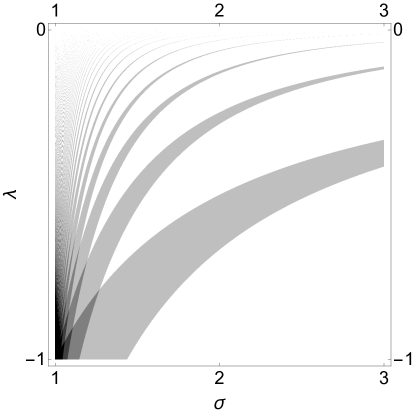
Figure 6: The number $k^{*}(\sigma,\lambda)$ of intervals $J_{k}$ is represented according to the following convention: white corresponds to $k^{*}=1$, light gray to $k^{*}=2$, gray to $k^{*}=3$, dark gray to $k^{*}=4$, black to $k^{*}\geq 5$. The number $k^{*}$ increases as $\lambda\to-1$ and $\sigma\to 1$.

Second, only the rightmost segment $J_{1}$ can have any of the types I, II or III. All the other segments (if they exist) are of type III. This observation suggests that the map (21) does not have segments of types I and II simultaneously, i.e. the asymptotically stable fixed point of the map (21) does not coexist with a chaotic invariant set of type (5) composed of a finite number of closed intervals. Fig. 7(a) shows the type of the interval $J_{1}$ (depending on the values of parameters $\lambda$ and $\sigma$) when $k^{*}\geq 2$. In this case, $J_{1}\not\subset J^{*}$. Similarly, Fig. 7(b) shows the type of the segment $J_{1}$ for the case $k^{*}=1$ when $J_{1}\subset J^{*}$.

Third, we found that if the rightmost interval $J_{1}$ is of type II, then the chaotic attractor $\Lambda_{k}$ contained in this interval is either a segment or a union of two disjoint segments (cf. (5)).

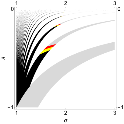
(a)

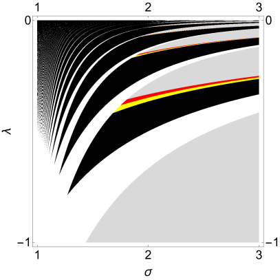
(b)

Figure 7: The type of the interval $J_{1}$ depending on the values of the parameters $\lambda$ and $\sigma$. $(a)$ $k^{*}\geq 2$ ($J_{1}\not\subset J^{*}$); $(b)$: $k^{*}=1$ ($J_{1}\subset J^{*}$). We adopt the following convention: light gray corresponds to type I, yellow to type II with the chaotic attractor $\Lambda_{k}\subset J_{k}$ consisting of one segment, red to type II with the chaotic attractor $\Lambda_{k}\subset J_{k}$ consisting two disjoint segments, black to type III, white on panel $(a)$ to $k^{*}=1$, white on panel $(b)$ to $k^{*}\geq 2$.

Note that the domain ${\mathcal{D}}$ of existence for the stable fixed point of $T$ (the rightmost segment $J_{1}$ is of type I) has been found in [2]:

$${\mathcal{D}}=\bigcup_{i=1}^{\infty}\left\{(\lambda,\sigma):\ \dfrac{\sigma^{i}-1}{\sigma-1}\leq-\frac{1}{\lambda}<\sigma^{i},\ \sigma>1,\ -1<\lambda<0\right\}.$$

Remark 9.

Any point $(x,1)\in l^{+}$ with $x\in(\hat{q}_{k+1},\hat{q}_{k})$ reaches the half-line $l^{-}$ in $k+1$ iterations under the map (14) [2]. This implies that every periodic orbit of $T$ corresponds to a periodic orbit of the map (14). In particular, since $J_{k}\subset(q_{k+1},q_{k})$, the fixed points $e_{k}$, $\hat{e}_{k}$ correspond to $(2(k+1))$-periodic orbits of (14). Stable orbits of $T$ correspond to stable orbits of (14).

Remark 10.

System (14) has been alternatively interpreted in [2] as follows. Let $s_{0}\in[-1,1]$ and let $\{x_{n}\}$, $n\in\mathbb{N}_{0}$, be a real-valued sequence. Consider the sequence

$$s_{n+1}=\Phi(s_{n}+x_{n+1}-x_{n}),\quad n\in\mathbb{N}_{0},$$

with the saturation function (15). The mapping of the pair $s_{0},\,\{x_{n}\}$ to the sequence $\{s_{n}\}$ according to this formula is known in different disciplines as the stop operator $\mathcal{S}$ [15, 6], Prandtl’s model of elastic-ideal plastic element [25], the backlash nonlinearity, and the one-dimensional Moreau sweeping process [18, 23]. Here $s_{0}$ is called the initial state, $\{x_{n}\}$ is called the input, $\{s_{n}\}={\mathcal{S}}[s_{0},\{x_{n}\}]$ is called the output (or, the variable state) of the stop operator. With this notation, system (14) is equivalent to the simple feedback loop coupling a linear unit with the stop operator:

$$\{x_{n+1}\}=\lambda\{x_{n}\}+(\sigma-\lambda){\mathcal{S}}[s_{0},\{x_{n}\}],$$

which is the interpretation used in [2].

References

- [1] A. A. Andronov, S. E. Khaikin, and A. A. Vitt. Theory of oscillators. Dover, 1966.
- [2] M. Arnold, N. Begun, P. Gurevich, E. Kwame, H. Lamba, and D. Rachinskii. Dynamics of discrete time systems with a hysteresis stop operator. SIAM Journal on Applied Dynamical Systems, 16(1):91–119, 2017.
- [3] V. Avrutin and I. Sushko. A gallery of bifurcation scenarios in piecewise smooth 1d maps. In Global Analysis of Dynamic Models in Economics and Finance, pages 369–395. Springer, 2013.
- [4] S. Banerjee, J. A. Yorke, and C. Grebogi. Robust chaos. Physical Review Letters, 80(14):3049, 1998.
- [5] M. Bernardo, C. Budd, A. R. Champneys, and P. Kowalczyk. Piecewise-smooth dynamical systems: theory and applications, volume 163. Springer Science & Business Media, 2008.
- [6] M. Brokate and J. Sprekels. Hysteresis and Phase Transitions. Springer-Verlag, New York, 1996.
- [7] W. De Melo and S. Van Strien. One-dimensional dynamics, volume 25. Springer Science & Business Media, 2012.
- [8] R. Devaney. An introduction to chaotic dynamical systems. Westview press, 2008.
- [9] M. di Bernardo, C. J. Budd, A. R. Champneys, P. Kowalczyk, A. B. Nordmark, G. O. Tost, and P. T. Piiroinen. Bifurcations in nonsmooth dynamical systems. SIAM Review, 50(4):629–701, 2008.
- [10] M. Feigin. Doubling of the oscillation period with c-bifurcations in piecewise-continuous systems. Journal of Applied Mathematics and Mechanics, 34(5):861–869, 1970.
- [11] A. Filippov. Differential equations with discontinuous righthand sides. Kluwer Academic Publishers, 1988.
- [12] L. Gardini, D. Fournier-Prunaret, and P. Chargé. Border collision bifurcations in a two-dimensional piecewise smooth map from a simple switching circuit. Chaos: An Interdisciplinary Journal of Nonlinear Science, 21(2):023106, 2011.
- [13] M. Göcke. Various concepts of hysteresis applied in economics. Journal of Economic Surveys, 16(2):167–188, 2002.
- [14] J. Guckenheimer and R. F. Williams. Structural stability of lorenz attractors. Publications Mathématiques de l’IHÉS, 50:59–72, 1979.
- [15] M. Krasnosel’skii and A. Pokrovskii. Systems with Hysteresis. Springer-Verlag, Berlin, 1989.
- [16] P. Krejčí, H. Lamba, S. Melnik, and D. Rachinskii. Analytical solution for a class of network dynamics with mechanical and financial applications. Physical Review E, 90(3):032822, 2014.
- [17] M. Kunze. Non-smooth dynamical systems, volume 1744. Springer Science & Business Media, 2000.
- [18] M. Kunze and M. Monteiro Marques. An introduction to Moreau’s sweeping process. In Impacts in mechanical systems (Grenoble, 1999), volume 551 of Lecture Notes in Phys., pages 1–60. Springer, Berlin, 2000.
- [19] N. Leonov. Map of the line onto itself. Radiofisica, 3(3):942–956, 1959.
- [20] D. V. Lyubimov, A. Pikovsky, and M. Zaks. Universal scenarios of transitions to chaos via homoclinic bifurcations, volume 8. CRC Press, 1989.
- [21] Y. L. Maistrenko, V. Maistrenko, and L. Chua. Cycles of chaotic intervals in a time-delayed chua’s circuit. International Journal of Bifurcation and Chaos, 3(06):1557–1572, 1993.
- [22] D. S. Meiss and JD. Neimark–sacker bifurcations in planar, piecewise-smooth, continuous maps. SIAM Journal on Applied Dynamical Systems, 7(3):795–824, 2008.
- [23] J.-J. Moreau. On unilateral constraints, friction and plasticity. In New variational techniques in mathematical physics (Centro Internaz. Mat. Estivo (C.I.M.E.), II Ciclo, Bressanone, 1973), pages 171–322. Edizioni Cremonese, Rome, 1974.
- [24] H. E. Nusse and J. A. Yorke. Border-collision bifurcations including “period two to period three” for piecewise smooth systems. Physica D: Nonlinear Phenomena, 57(1-2):39–57, 1992.
- [25] L. Prandtl. Ein Gedankenmodell zur kinetischen Theorie der festen Körper. ZAMM-Journal of Applied Mathematics and Mechanics/Zeitschrift für Angewandte Mathematik und Mechanik, 8(2):85–106, 1928.
- [26] D. J. W. Simpson. Bifurcations in piecewise-smooth continuous systems, volume 70. World Scientific, 2010.
- [27] I. Sushko, V. Avrutin, and L. Gardini. Bifurcation structure in the skew tent map and its application as a border collision normal form. Journal of Difference Equations and Applications, 22(8):1040–1087, 2016.
- [28] I. Sushko and L. Gardini. Degenerate bifurcations and border collisions in piecewise smooth 1d and 2d maps. International Journal of Bifurcation and Chaos, 20(07):2045–2070, 2010.
- [29] Z. T. Zhusubaliyev and E. Mosekilde. Bifurcations And Chaos In Piecewise-Smooth Dynamical Systems: Applications to Power Converters, Relay and Pulse-Width Modulated Control Systems, and Human Decision-Making Behavior, volume 44. World Scientific, 2003.