Implicit Regularization in Deep Learning
by
Behnam Neyshabur
A thesis submitted
in partial fulfillment of the requirements for
the degree of
Doctor of Philosophy in Computer Science
at the
TOYOTA TECHNOLOGICAL INSTITUTE AT CHICAGO
August, 2017
Thesis Committee:
Nathan Srebro (Thesis advisor),
Yury Makarychev,
Ruslan Salakhutdinov,
Gregory Shakhnarovich

See pages - of sign.pdf

Implicit Regularization in Deep Learning
by
Behnam Neyshabur

Abstract

In an attempt to better understand generalization in deep learning, we study several possible explanations. We show that implicit regularization induced by the optimization method is playing a key role in generalization and success of deep learning models. Motivated by this view, we study how different complexity measures can ensure generalization and explain how optimization algorithms can implicitly regularize complexity measures. We empirically investigate the ability of these measures to explain different observed phenomena in deep learning. We further study the invariances in neural networks, suggest complexity measures and optimization algorithms that have similar invariances to those in neural networks and evaluate them on a number of learning tasks.

Thesis Advisor: Nathan Srebro
Title: Professor

In memory of my dear friend, Sina Masihabadi

Acknowledgments

I would like to thank my advisor Nati Srebro without whom I would not be even pursuing a PhD in the first place. Nati’s classes made me interested in optimization and machine learning and later I was delighted when he agreed to be my advisor. From the very first few meetings, I realized how his excitement and passion for research energizes me. I will not forget our countless long meetings that did not seem long to me at all. Looking back, I think Nati was the best mentor I could have hoped for. Among the skills I started to pick up from Nati, my favorite is asking the right question and formalizing it. About three years ago, excited about recent advances in deep learning, I walked into Nati’s office and I told him that I want to understand what makes deep learning models perform well in practice. He helped me to ask the right questions and formalize them. Nati has had a great influence in shaping my thoughts and therefore this dissertation. I am forever grateful for all I have learned from him.

I would like to thank all of my committee members from whom I benefited during my PhD study. I am thankful to Ruslan Salakhutdinov who has been advising me in several projects and I have benefited a lot from discussions with him and his advices regarding my career. I thank Yury Makarychev for his collaborations and advices during early years of PhD. I always felt free to knock at his office door whenever I was stuck with theoretical questions and needed more insight. I thank Greg Shakhnarovich who has been kind enough to answer my questions on deep learning and metric learning whenever I showed up at his office. Moreover, I think his well-prepared machine learning course had a great impact on making me interested in machine learning.

TTIC’s faculty have a close and friendly relationship with students and I have benefited from that. I am thankful to Jinbo Xu, my interim advisor who encouraged me to continue PhD in the area that fits my interests the best. I am pleased that we continued collaboration on computational biology projects. Madhur Tulsiani deserves a special thanks for being a great director of graduate studies. Madhur’s desire to improve the PhD program at TTIC and his support made me feel comfortable and free to discuss my thoughts and suggestions with him many times. I would like to acknowledge that I really enjoyed the mathematical foundation course taught by David McAllester and his views on deep learning which he discussed in his deep learning course at TTIC. I regret that I only started collaborating with him in last few months of my PhD and I wish I would have had more discussions with him during these years. I was not able to collaborate with Karen Livescu and Kevin Gimpel during my PhD years but I have enjoyed many conversations with them and I felt supported by them. I also thank Sadaoki Furui, Julia Chuzhoy and Matthew Walter for their effort in enhancing TTIC’s PhD program. I had the pleasure of chatting with Avrim Blum a few times since he has joined TTIC and I am excited about his new appointment at TTIC.

During my PhD years, I have enjoyed collaborating with several research faculties at TTIC. I would like to thank Srinadh Bhojanapalli with whom I have spent a lot of time in the last two years for being a good friend, mentor and collaborator. I am very grateful for everything he has offered me. My earlier works in deep learning was in collaboration with Ryota Tomioka and I am thankful his help and support. Suriya Gunasekar is another research faculty at TTIC who has been an amazing friend and collaborator. Other than her help and support, I have also enjoyed countless discussions with her on random topics. I would like to thank Aly Khan and Ayan Chakrabarti for what I have learned from them during our collaborations on different projects. Finally, I have learned from and enjoyed chatting with many other research faculty and postdocs at TTIC including but not limited to Michael Maire, Hammad Naveed, Mesrob Ohannessian, Mehrdad Mahdavi, Weiran Wang, Herman Kamper, Ofer Meshi, Qixing Huangi, Subhransu Maji, Raman Arora, and George Papandreou.

I would like to thank TTIC students. I am indebted to Payman Yadollahpour who kindly hosted me and my wife, Somaye, for several days after we arrived to US and helped us numerous times in various occasions. I am grateful for knowing him and for all the moments we have shared. Hao Tang also deserves a special thanks. He was the person I used to discuss all my ideas and thoughts with. Therefore, everything presented in this thesis is somehow impacted by the discussions with him. I thank Mrinalkanti Ghosh for the countless times I interrupted his work with a theoretical question and he patiently helped me try to investigate it. Shubhendu Trivedi is another student whom I had several fruitful discussion with. I am also thankful for things I have learned from and memories I have shared with Bahador Nooraei, Mohammadreza Mostajabi, Haris Angelidakis, Vikas Garg, Kaustav Kundu, Abhishek Sen, Siqi Sun, Hai Wang, Heejin Choi, Qingming Tang, Lifu Tu, Blake Woodworth, Shubham Toshniwal, Shane Settle, Nicholas Kolkin, Falcon Dai, Charles Schaff, Rachit Nimavat, and Ruotian Luo.

I want to thank TTIC staff for making my life much easier and helping me whenever I had any problems. On top of the list is Chrissy Novak. She has always patiently and kindly listened to my complaints, suggestions, and problems, and tried her best to resolve or improve any issues. Adam Bohlander has always been helpful and quick in resolving any IT issues. I think Adam’s great expertise has saved me several hundreds of hours. Liv Leader was one of TTIC’s staff when we arrived to US. She helped us during the first few months of being in US. The first party we were invited in US was Liv’s housewarming party. I also thank Mary Marre, Amy Minick, Jessica Johnston and other TTIC staffs for their effort.

Beyond TTIC, I am grateful for my internship at MSR Silicon Valley with Rina Panigrahy. Perhaps, several hundred hours of meeting and discussions with Rina in this internship whose goal was to better understand neural networks theoretically had a great influence on making me interested in deep learning. I am also thankful for collaboration and discussions I had with Robert Schapire, Alekh Agarwal, Haipeng Luo and John Langford during my internship at MSR New York City. I am grateful to Anna Choromanska for several discussions on neural networks and for great career advices I received from her. I thank Tony Wu for being a good friend and collaborator. I have learned a lot about deep learning from several meetings with him.

My deepest gratitude goes to my parents and my brother who have shaped who I am today. Words cannot capture how grateful I am to Somaye without whom everything in my life would have been drastically different. I will thank her in person.

I am dedicating this thesis to the memory of my dear friend Sina Massihabadi who went to the same high school and university as me. Sina was very brilliant and one of the finest human beings I have ever met. Later, he moved to United States to start a PhD in industrial engineering at Texas A&M university. However, he did not make it to the end of the program. He died in a tragic car accident when he was driving to the airport to pick up his mother whom he was not able to visit for two years due to visa restrictions on Iranians.

Contents

1. 1 Introduction
   1. 1.1 Main Contributions
2. 2 Preliminaries
   1. 2.1 The Statistical Learning Framework
   2. 2.2 Feedforward Neural Networks with Shared Weights
3. I Implicit Regularization and Generalization
   1. 3 Generalization and Capacity Control
      1. 3.1 VC Dimension: A Cardinality-Based Arguments
      2. 3.2 Norms and Margins: Counting Real-Valued Functions
      3. 3.3 Robustness: Lipschitz Continuity with Respect to Input
      4. 3.4 PAC-Bayesian Framework: Sharpness with Respect to Parameters
   2. 4 On the Role of Implicit Regularization in Generalization
      1. 4.1 Network Size and Generalization
      2. 4.2 A Matrix Factorization Analogy
   3. 5 Norm-based Capacity Control
      1. 5.1 Group Norm Regularization
      2. 5.2 Per-Unit and Path Regularization
      3. 5.3 Overall Regularization
      4. 5.4 Depth Independent Regularization
      5. 5.5 Proofs
      6. 5.6 Discussion
   4. 6 Sharpness/PAC-Bayes Generalization Bounds
      1. 6.1 Spectrally-Normalized Margin Bounds
      2. 6.2 Generalization Bound based on Expected Sharpness
      3. 6.3 Supporting Results
      4. 6.4 Proofs
   5. 7 Empirical Investigation
      1. 7.1 Complexity Measures
      2. 7.2 Experiments Settings
      3. 7.3 True Labels Vs. Random Labels
      4. 7.4 Different Global Minima
      5. 7.5 Increasing Network Size
4. II Geometry of Optimization and Generalization
   1. 8 Invariances
      1. 8.1 Invariances in Feedforward and Recurrent Neural Networks
      2. 8.2 Understanding Invariances

List of Figures

1. 4.1 The training and test error of a two-layer perceptron for varying number of hidden units
2. 4.2 The generalization behavior a two-layer perceptron for varying number of hidden units
3. 6.1 Verifying the conditions of Theorem a multi-layer perceptron
4. 6.2 Condition $C1$ in Theorem a learned network.
5. 6.3 Ratio of activations that flip based on the magnitude of perturbation.
6. 6.4 Condition $C3$ in Theorem r random initialization and learned network
7. 7.1 Comparing complexity measures on a VGG network trained with true or random labels.
8. 7.2 Sharpness and PAC-Bayes measures on a VGG network trained with true or random labels.
9. 7.3 Experiments on global minima with poor generalization.
10. 7.4 The effect of increasing network size on generalization.
11. 8.1 Invariance in fully connected feedforward networks
12. 8.2 Invariances in recurrent neural networks (RNNs).

List of Tables

1. 2.1 Forward computations for feedforward and recurrent networks

Chapter 1 Introduction

Deep learning refers to training typically complex and highly over-parameterized models that benefit from learning a hierarchy of representations. The terms “neural networks” and “deep learning” are often used interchangeably as many modern deep learning models are slight modifications of different types of neural networks suggested originally around 1950-2000 [schimidhuber15]. Interest in deep learning was revived around 2006  [hinton06, bengio07] and since then, it has had enormous practical successes in different areas [lecun15]. The rapid growth of practical works and new concepts in this field has created a considerable gap between our theoretical understanding of deep learning and practical advances.

From the learning viewpoint, we often look into three different properties to investigate the effectiveness of a model: expressive power, optimization, and generalization. Given a function class/model the expressive power is about understanding what functions can be realized or approximated by the functions in the function class. Given a loss function as an evaluation measure, the optimization aspect refers to the ability to efficiently find a function with a minimal loss on the training data and generalization addresses the model’s ability to perform well on the new unseen data.

All above aspects of neural networks have been studied before. Neural networks have great expressive power. Universal approximation theorem states that for any given precision, feed-forward networks with a single hidden layer containing a finite number of hidden units can approximate any continuous function [hornik1989multilayer]. More broadly, any $O(T)$ time computable function can be captured by an $O(T^{2})$ sized network, and so the expressive power of such networks is indeed great [sipser2012, Theorem 9.25].

Generalization of neural networks as a function of network size is also fairly well understood. With hard-threshold activations, the VC-dimension, and hence sample complexity, of the class of functions realizable with a feed-forward network is equal, up to logarithmic factors, to the number of edges in the network [anthony09, shalev14], corresponding to the number of parameters. With continuous activation functions the VC-dimension could be higher, but is fairly well understood and is still controlled by the size of the network.

At the same time, we also know that learning even moderately sized networks is computationally intractable—not only is it NP-hard to minimize the empirical error, even with only three hidden units, but it is hard to learn small feed-forward networks using any learning method (subject to cryptographic assumptions). That is, even for binary classification using a network with a single hidden layer and a logarithmic (in the input size) number of hidden units, and even if we know the true targets are exactly captured by such a small network, there is likely no efficient algorithm that can ensure error better than 1/2 [klivans2006cryptographic, Daniely14]—not if the algorithm tries to fit such a network, not even if it tries to fit a much larger network, and in fact no matter how the algorithm represents predictors. And so, merely knowing that some not-too-large architecture is excellent in expressing does not explain why we are able to learn using it, nor using an even larger network. These results, however, are not suggesting any insights on the practical success of deep learning. In contrast to our theoretical understanding, it is possible to train (optimize) very large neural networks and despite their large sizes, they generalize to unseen data. Why is it then that we succeed in learning very large neural networks? Can we identify a property that makes them possible to train? Why do these networks generalize to unseen data despite their large capacity in terms of the number of parameters?

In such an over-parameterized setting, the objective has multiple global minima, all minimize the training error, but many of them do not generalize well. Hence, just minimizing the training error is not sufficient for learning: picking the wrong global minima can lead to bad generalization behavior. In such situations, generalization behavior depends implicitly on the algorithm used to minimize the training error. Different algorithmic choices for optimization such as the initialization, update rule, learning rate, and stopping condition, will lead to different global minima with different generalization behavior [chaudhari2016entropy, keskar2016large, NeySalSre15].

What is the bias introduced by these algorithmic choices for neural networks? What is the relevant notion of complexity or capacity control?

The goal of this dissertation is to understand the implicit regularization by studying the optimization, regularization, and generalization in deep learning and the relationship between them. The dissertation is divided into two parts. In the first part, we study different approaches to explain generalization in neural networks. We discuss how some of the complexity measures derived by these approaches can explain implicit regularization. In the second part, we investigate the transformations under which the function computed by a network remains the same and therefore argue for complexity measures and optimization algorithms that have similar invariances. We find complexity measures that have similar invariances to neural networks and optimization algorithms that implicitly regularize them. Using these optimization algorithms for different learning tasks, we indeed observe that they have better generalization abilities.

1.1 Main Contributions

1. Part I:

   1. The Role of Implicit Regularization (Chapter 4) We design experiments to highlight the role of implicit regularization in the success of deep learning models.

   2. Norm-based capacity control (Chapter 5): We prove generalization bounds for the class of fully connected feedforward networks with the bounded norm. We further show that for some norms, this bound is independent of the number of hidden units.

   3. Generalization Guarantee by PAC-Bayes Framework (Chapter 6): We show how PAC-Bayes framework can be employed to obtain generalization bounds for neural networks by making a connection between sharpness and PAC-Bayes theory.

   4. Implicit Regularization by SGD (Chapter 6): We show that networks learned by SGD satisfy several conditions that lead to flat minima.

   5. Empirical Investigation of Generalization in Deep Learning (Chapter 7): We design experiments to compare the ability of different complexity measures to explain the implicit regularization and generalization in deep learning.

2. Part II:

   1. Invariances in neural networks (Chapter 8): We characterize a large class of invariances in feedforward and recurrent neural networks caused by rescaling issues and suggest a measure called the Path-norm that is invariant to the rescaling of the weights.

   2. Path-normalized optimization (Chapter 9 and 10): Inspired by our understanding of invariances in neural networks and the importance of implicit regularization, we suggest a new method called Path-SGD whose updates are the approximate steepest descent direction with respect to the Path-norm. We show Path-SGD achieves better generalization error than SGD in both fully connected and recurrent neural networks on different benchmarks.

   3. Data-dependent path normalization (Chapter 11): We propose a unified framework for neural net normalization, regularization, and optimization, which includes Path-SGD and Batch-Normalization and interpolates between them across two different dimensions. Through this framework, we investigate the issue of invariance of the optimization, data dependence and the connection with natural gradient.

Chapter 2 Preliminaries

In this chapter, we present the basic setup and notations used throughout this dissertation.

2.1 The Statistical Learning Framework

In this section, we briefly review the statistical learning framework. More details on the formal model can be found in shalev14.

In the statistical batch learning framework, the learner is given a training set $\mathcal{S}=\{(\mathbf{x}_{1},\mathbf{y}_{1}),\dots,(\mathbf{x}_{m},\mathbf{y}_{m})\}$ of $m$ training points in $\mathcal{X}\times\mathcal{Y}$ that are independently and identically distributed (i.i.d.) according to an unknown distribution $\mathcal{D}$. For simplicity, we will focus on the task of classification where the goal of the learner is to output a predictor $f:\mathcal{X}\rightarrow\mathcal{Y}$ with minimum expected error on samples generated from the distribution $\mathcal{D}$:

$$L_{\mathcal{D}}(f)={\mathbb{P}_{(\mathbf{x},\mathbf{y})\sim\mathcal{D}}\left[{f(\mathbf{x})\neq\mathbf{y}}\right]}$$ (2.1.1)

Since the learner does not have access to the distribution $\mathcal{D}$, it cannot evaluate or minimize the expected loss. It can however, obtain an estimate of the expected loss of a predictor $f$ using the training set $\mathcal{S}$:

$$L_{\mathcal{S}}(f)=\frac{{\left\lvert{\left\{(\mathbf{x},\mathbf{y})\in\mathcal{S}\mid f(\mathbf{x})\neq\mathbf{y}\right\}}\right\rvert}}{m}$$ (2.1.2)

When the distribution $\mathcal{D}$ and training set $\mathcal{S}$ is clear from the context, we use $L(f)$ and $\hat{L}(f)$ instead of $L_{\mathcal{D}}$ and $L_{\mathcal{S}}(f)$ respectively. We also define the expected margin loss for any margin $\gamma>0$, as follows:

$$L_{\gamma}(f)={\mathbb{P}_{(\mathbf{x},y)\sim\mathcal{D}}\left[{f(\mathbf{x})[y]\leq\gamma+\max_{j\neq y}f(\mathbf{x})[j]}\right]}$$ (2.1.3)

Let $\hat{L}_{\gamma}(f)$ be the empirical estimate of the above expected margin loss. Since setting $\gamma=0$ corresponds to the classification loss, we will use $L_{0}(f)=L(f)$ and $\hat{L}_{0}(f_{\mathbf{w}})=\hat{L}(f)$ to refer to the expected risk and the training error.

Minimizing the loss in the equation (2.1.2) which is called the training error does not guarantee low expected error. For example, a predictor that only memorizes the set $\mathcal{S}$ to output the right label for the data in the training set can get zero training error while its expected loss might be very close to the random guess. We are therefore interested in controlling the difference $L_{\mathcal{D}}(f)-L_{\mathcal{S}}(f)$ which we will refer to as generalization error. This quantity reflects the difference between memorizing and learning.

An interesting observation is that if $f$ is chosen in advance and is not dependent on the distribution $\mathcal{D}$ or training set $\mathcal{S}$, then the generalization error can be simply bounded by concentration inequalities such as Hoeffding’s inequality and relatively small number of samples are required to get small generalization error. However, since the predictor is chosen by the learning algorithm using the training set $\mathcal{S}$, one need to make sure that this bound holds for the set all predictors that could be chosen by the learning algorithm. It is therefore preferred to limit the search space of the learning algorithm to a small enough set $\mathcal{F}$ of predictors called model class to be able to bound the generalization.

We consider the statistical capacity of a model class in terms of the number of examples required to ensure generalization, i.e. that the population (or test error) is close to the training error, even when minimizing the training error. This also roughly corresponds to the maximum number of examples on which one can obtain small training error even with random labels.

In the next section, we define a meta-model class of feedforward networks with shared weights that include several well-known model classes such as fully connected, convolutional and recurrent neural networks.

2.2 Feedforward Neural Networks with Shared Weights

We denote a feedforward network by a triple $(G,\mathbf{w},\sigma)$ where $G=(V,E)$ is a directed acyclic graph over the set of nodes $V$ that corresponds to units $v\in V$ in the network, including special input nodes $V_{\text{in}}\subset V$ with no incoming edges and special output nodes $V_{\text{out}}\subseteq V$ with no outgoing edges, $\mathbf{w}:E\rightarrow\mathbb{R}$ is the weights assigned to the edges and $\sigma:\mathbb{R}\rightarrow\mathbb{R}$ is an activation function.

Feedforward network $(G,\mathbf{w},\sigma)$ computes the function $f_{G,\mathbf{w},\sigma}:\mathbb{R}^{n_{\text{in}}}\rightarrow\mathbb{R}^{n_{\text{out}}}$ for a given input vector $\mathbf{x}\in\mathbb{R}^{n_{\text{in}}}$ as follows: For any input node $v\in V_{\text{in}}$, its output $h_{v}$ is the corresponding coordinate of $\mathbf{x}$ ; for any internal node $v$ (all nodes except the input and output nodes) the output value is defined according to the forward propagation equation:

$$h_{v}=\sigma\left(\sum_{(u\rightarrow v)\in E}w_{u\rightarrow v}\cdot h_{u}\right)$$ (2.2.1)

and for any output node $v\in V_{\text{out}}$, no non-linearity is applied and its output $h_{v}=\sum_{(u\rightarrow v)\in E}w_{u\rightarrow v}\cdot h_{u}$ corresponds to coordinates of the computed function $f_{G,\mathbf{w},\sigma}(\mathbf{x})$. When the graph structure $G$ and the activation function $\sigma$ is clear from the context, we use the shorthand $f_{\mathbf{w}}=f_{G,\mathbf{w},\sigma}$ to refer to the function computed by weights $\mathbf{w}$.

We will focus mostly on the hinge, or RELU (REctified Linear Unit) activation, which is currently in popular use [nair10, glorot11, zeiler13], $\sigma_{\textsc{relu}}(z)=[z]_{+}=\max(z,0)$. When the activation will not be specified, we will implicitly be referring to the RELU. The RELU has several convenient properties which we will exploit, some of them shared with other activation functions:

Lipshitz

ReLU is Lipschitz continuous with Lipschitz constant one. This property is also shared by the sigmoid and the ramp activation $\sigma(z)=\min(\max(0,z),1)$.

Idempotency

ReLU is idempotent, i.e. $\sigma_{\textsc{relu}}(\sigma_{\textsc{relu}}(z))=\sigma_{\textsc{relu}}(z)$. This property is also shared by the ramp and hard threshold activations.

Non-Negative Homogeneity

For a non-negative scalar $c\geq 0$ and any input $z\in\mathbb{R}$ we have $\sigma_{\textsc{relu}}(c\cdot z)=c\cdot\sigma_{\textsc{relu}}(z)$. This property is important as it allows us to scale the incoming weights to a unit by $c>0$ and scale the outgoing edges by $1/c$ without changing the function computed by the network. For layered graphs, this means we can scale $\mathbf{W}^{i}$ by $c$ and compensate by scaling $\mathbf{W}^{i+1}$ by $1/c$.

When investigating a class of feedforward networks, in order to account for weight sharing, we separate the weights from actual parameters. Given a parameter vector $\bm{\theta}\in\mathbb{R}^{n}_{\text{param}}$ and a mapping $\pi:E\rightarrow\{1,\dots,n_{\text{param}}\}$ from edges to parameter indices, the weight of any edge $e\in E$ is $w_{e}=\theta_{\pi(e)}$. We also refer to the set of edges that share the $i$th parameter $\theta_{i}$ as $E_{i}=\left\{e\in E|\pi(e)=i\right\}$. That is, for any $e_{1},e_{2}\in E_{i}$, $\pi(e_{1})=\pi(e_{2})$ and therefore $w_{e_{1}}=w_{e_{2}}=\theta_{\pi(e_{1})}$. Given a graph $G$, activation function $\sigma$ and mapping $\pi$, we consider the hypothesis class $\mathcal{F}^{G,\sigma,\pi}=\left\{f_{G,w,\sigma}|\bm{\theta}\in\mathbb{R}^{k};\forall_{e\in E}\;w(e)=\theta_{\pi(e)}\right\}$ of functions computable using some setting of parameters. When $\pi$ is a one-to-one mapping, we use weights $\mathbf{w}$ to refer to the parameters $\bm{\theta}$ and drop $\pi$ and use $\mathcal{F}^{G,\sigma}$ to refer to the hypothesis class.

We will refer to the size of the network, which is the overall number of edges $n_{\text{edge}}={\left\lvert{E}\right\rvert}$, the depth $d$ of the network, which is the length of the longest directed path in $G$, and the in-degree (or width) $H$ of a network, which is the maximum in-degree of a vertex in $G$.

If the mapping $\pi$ is a one-to-one mapping, then there is no weight sharing and it corresponds to standard feedforward networks. Fully connected neural networks (FCNNs) are a well-known family of standard feedforward networks in which every hidden unit in each layer is connected to all hidden units in the previous and next layers. On the other hand, weight sharing exists if $\pi$ is a many-to-one mapping. Two well-known examples of feedforward networks with shared weights are convolutional neural networks (CNNs) and recurrent neural networks (RNNs). We mostly use the general notation of feedforward networks with shared weights as this will be more comprehensive. However, when focusing on FCNNs or RNNs, it is helpful to discuss them using a more familiar notation which we briefly introduce next.

Fully Connected Neural Networks

Let us consider a layered fully-connected network where nodes are partitioned into layers. Let $n_{i}$ be the number of nodes in layer $i$. For all nodes $v$ on layer $i$, we recover the layered recursive formula $\mathbf{h}^{i}=\sigma\left(\mathbf{W}^{i}\mathbf{h}^{i-1}\right)$ where $\mathbf{h}^{i}\in\mathbb{R}^{n_{i}}$ is the vector of outputs in layer $i$ and $\mathbf{W}^{i}\in\mathbb{R}^{n_{i}\times n_{i-1}}$ is the weight matrix in layer $i$ with entries $w_{u\rightarrow v}$, for each $u$ in layer $i-1$ and $v$ in layer $i$. This description ignores the bias term, which could be modeled as a direct connection from $v_{\rm bias}$ into every node on every layer, or by introducing a bias unit (with output fixed to 1) at each layer.

Recurrent Neural Networks

Time-unfolded RNNs are feedforward networks with shared weights that map an input sequence to an output sequence. Each input node corresponds to either a coordinate of the input vector at a particular time step or a hidden unit at time $0$. Each output node also corresponds to a coordinate of the output at a specific time step. Finally, each internal node refers to some hidden unit at time $t\geq 1$. When discussing RNNs, it is useful to refer to different layers and the values calculated at different time-steps. We use a notation for RNN structures in which the nodes are partitioned into layers and $\mathbf{h}_{t}^{i}$ denotes the output of nodes in layer $i$ at time step $t$. Let $\mathbf{x}=(\mathbf{x}_{1},\dots,\mathbf{x}_{T})$ be the input at different time steps where $T$ is the maximum number of propagations through time and we refer to it as the length of the RNN. For $0\leq i<d$, let $\mathbf{W}_{\text{in}}^{i}\in\mathbb{R}^{n_{i}\times n_{i-1}}$ and $\mathbf{W}_{\text{rec}}^{i}\in\mathbb{R}^{n_{i}\times n_{i}}$ be the input and recurrent parameter matrices of layer $i$ and $\mathbf{W}_{\text{out}}\in\mathbb{R}^{n_{d}\times n_{d-1}}$ be the output parameter matrix.The output of the function implemented by RNN can then be calculated as $f_{\mathbf{w},t}(x)=h_{t}^{d}$. Note that in this notations, weight matrices $\mathbf{W}_{\text{in}}$, $\mathbf{W}_{\text{rec}}$ and $\mathbf{W}_{\text{out}}$ correspond to “free” parameters of the model that are shared in different time steps. Table ows forward computations for layered feedforward networks and RNNs.

	Input nodes	Internal nodes	Output nodes
FF (shared weights)	$h_{v}=x[v]$	$h_{v}=\sigma\left(\sum_{(u\rightarrow v)\in E}w_{u\rightarrow v}h_{u}\right)$	$h_{v}=\sum_{(u\rightarrow v)\in E}w_{u\rightarrow v}h_{u}$
FCNN notation	$\mathbf{h}^{0}=\mathbf{x}$	$\mathbf{h}^{i}=\sigma\left(\mathbf{W}^{i}\mathbf{h}^{i-1}\right)$	$\mathbf{h}^{d}=\mathbf{W}^{d}\mathbf{h}^{d-1}$
RNN notation	$\mathbf{h}_{t}^{0}=\mathbf{x}_{t},\textbf{h}_{0}^{i}=0$	$\mathbf{h}_{t}^{i}=\sigma\left(\mathbf{W}_{\text{in}}^{i}\mathbf{h}_{t}^{i-1}+\mathbf{W}_{\text{rec}}^{i}\mathbf{h}_{t-1}^{i}\right)$	$\mathbf{h}_{t}^{d}=\mathbf{W}_{\text{out}}\mathbf{h}_{t}^{d-1}$

Table 2.1: Forward computations for feedforward nets with shared weights.

Part I Implicit Regularization and Generalization

Chapter 3 Generalization and Capacity Control

In section briefly discussed viewing the statistical capacity of a model class in terms of the number of examples required to ensure generalization. Given a model class $\mathcal{F}$, such as all the functions representable by some feedforward or convolutional networks, one can consider the capacity of the entire class $\mathcal{F}$—this corresponds to learning with a uniform “prior” or notion of complexity over all models in the class. Alternatively, we can also consider some complexity measure, which we take as a mapping that assigns a non-negative number to every predictor in the class - $\mu:\{\mathcal{F},\mathcal{S}\}\rightarrow\mathbb{R}^{+}$, where $\mathcal{S}$ is the training set. It is then sufficient to consider the capacity of the restricted class $\mathcal{F}_{\mu,\alpha}=\{f:f\in\mathcal{F},\mu(f)\leq\alpha\}$ for a given $\alpha\geq 0$. One can then ensure generalization of a learned predictor $f$ in terms of the capacity of $\mathcal{F}_{\mu,\mu(f)}$. Having a good predictor with low complexity, and being biased toward low complexity (in terms of $\mu$) can then be sufficient for learning, even if the capacity of the entire $\mathcal{F}$ is high. And if we are indeed relying on $\mu$ for ensuring generalization (and in particular, biasing toward models with lower complexity under $\mu$), we would expect a learned $f$ with a lower value of $\mu(f)$ to generalize better.

For some complexity measures, we allow $\mu$ to depend also on the training set. If this is done carefully, we can still ensure generalization for the restricted class $\mathcal{F}_{\mu,\alpha}$.

When considering a complexity measure $\mu$, we can investigate whether it is sufficient for generalization, and analyze the capacity of $\mathcal{F}_{\mu,\alpha}$. Understanding the capacity corresponding to different complexity measures also allows us to relate between different measures and provides guidance as to what and how we should measure: From the above discussion, it is clear that any monotone transformation of a complexity measures leads to an equivalent notion of complexity. Furthermore, complexity is meaningful only in the context of a specific model class $\mathcal{F}$, e.g. specific architecture or network size. The capacity, as we consider it (in units of sample complexity), provides a yardstick by which to measure complexity (we should be clear though, that we are vague regarding the scaling of the generalization error itself, and only consider the scaling in terms of complexity and model class, thus we obtain only a very crude yardstick sufficient for investigating trends and relative phenomena, not a quantitative yardstick).

We next look at different ways of controlling the capacity.

3.1 VC Dimension: A Cardinality-Based Arguments

Consider a finite model class $\mathcal{F}$. Given any predictor $f\in\mathcal{F}$, training error $L(f)$ is the average of independent random variables and the expected error the excepted value of the training error. We can therefore use Hoeffding’s inequality upper bounds the generalization error with high probability:

$${\mathbb{P}\left[{L(f)-\hat{L}(f)\geq t}\right]}\leq e^{-2mt^{2}}$$ (3.1.1)

The above bound is for any given $f$. However, since the learning algorithm can output any predictor from class $\mathcal{F}$, we need to make sure that all predictors in $\mathcal{F}$ have low generalization error which can be done through a union bound over model class $\mathcal{F}$:

$${\mathbb{P}\left[{\exists_{f\in\mathcal{F}}\;L(f)-\hat{L}(f)\geq t}\right]}\leq\sum_{f\in\mathcal{F}}{\mathbb{P}\left[{L(f)-\hat{L}(f)\geq t}\right]}\leq{\left\lvert{\mathcal{F}}\right\rvert}e^{-2mt^{2}}$$ (3.1.2)

Setting the r.h.s. of the above inequality to small probability $0<\delta<1$, we can say that with probability $1-\delta$ over the choice of samples in the training set, the following generalization bound holds:

$$L(f)\leq\hat{L}(f)+\sqrt{\frac{\ln{\left\lvert{\mathcal{F}}\right\rvert}+\ln(1/\delta)}{m}}$$ (3.1.3)

The above simple yet effective approach gives us an intuition about the relationship between the capacity and generalization. Many of the approaches of controlling the capacity that we will study later follow similar arguments. Here, the term $\ln{\left\lvert{\mathcal{F}}\right\rvert}$ corresponds to the complexity of the model class.

Even though many model classes that we consider are not finite based on the definition, one can argue that all parametrized model classes used in practice are finite since the parameters are stored with finite precision For any model, if $b$ bits are used to store each parameter, then we have $\ln{\left\lvert{\mathcal{F}}\right\rvert}\leq bn_{\text{param}}$ which is is linear in the total number of parameters.

Even without making an assumption on the precision of parameters, it is possible to get similar generalization bound using Vapnik-Chervonenkis dimension (VC dimension) which can be thought as the logarithm of the“intrinsic” cardinality. VC-dimension is defined as the size of the largest set $\mathcal{W}=\{\mathbf{x}_{i}\}_{i=1}^{m}$ such that for any mapping $g:\mathcal{W}\rightarrow\{\pm\}^{m}$, there is a predictor in $\mathcal{F}$ that achieves zero training error on the training set $\mathcal{S}=\left\{(\mathbf{x}_{i},g(\mathbf{x}_{i})\mid\mathbf{x}_{i}\in\mathcal{W}\right\}$. The VC-dimension of many known model classes is a linear or low-degree polynomial of the number of parameters. The following generalization bound then holds with probability $1-\delta$ [vapnik1971uniform, blumer1987occam]:

$$L(f)\leq\hat{L}(f)+\mathcal{O}\left(\sqrt{\frac{\text{VC-dim}(\mathcal{F})\ln m+\ln(1/\delta)}{m}}\right)$$ (3.1.4)

Feedforward Networks

The VC dimension of feedforward networks can also be bounded in terms of the number of parameters $n_{\text{param}}$[anthony2009neural, bartlett1998sample, bartlett1998almost, shalev2014understanding]. In particular, bartlet2017 and harvey2017nearly, following bartlett1998almost, give the following tight (up to logarithmic factors) bound on the VC dimension and hence capacity of feedforward networks with ReLU activations:

$$\text{VC-dim}=\tilde{O}(d*n_{\text{param}})$$ (3.1.5)

In the over-parametrized settings, where the number of parameters is more than the number of samples, complexity measures that depend on the total number of parameters are too weak and cannot explain the generalization behavior. Neural networks used in practice often have significantly more parameters than samples, and indeed can perfectly fit even random labels, obviously without generalizing [zhang2017understanding]. Moreover, measuring complexity in terms of number of parameters cannot explain the reduction in generalization error as the number of hidden units increase [neyshabur15b]. We will discuss more details about network size as the capacity control in Chapter 

3.2 Norms and Margins: Counting Real-Valued Functions

The model classes that we learn are often functions with real-valued outputs and for each task, we use a different loss and prediction method based on the predicted scores. For example, for the binary classification, thresholding the only real-valued output gives us the binary labels. For the multi-class classification, the output dimension is usually equal to the number of classes and the class with maximum score is chosen as the predicted label. For simplicity, we focus on binary classification here. Since the model class has real-valued output, can not directly use VC-dimension here. Instead, we can use a similar concept called subgraph VC-dimension which is similar to VC-dimension with the difference being that here we count the number of different behavior with a given margin. This means for the binary case, we require $yf(\mathbf{x})\geq\eta$ for some margin $\eta$. There are different techniques that bound subgraph-VC dimension such as Covering Numbers and Rademacher Complexities. Here, we focus on the Rademacher Complexity since most of the results by Covering Numbers can be also proved through Rademacher complexities with less effort. The empirical Rademacher complexity of a class $\mathcal{F}$ of function mapping from $\mathcal{X}$ to $\mathbb{R}$ with respect to a set $\{x_{1},\dots,x_{m}\}$ is defined as:

$$\mathcal{R}_{m}(\mathcal{F})={\mathbb{E}_{\xi\in\{\pm 1\}^{m}}\left[{\frac{1}{m}\sup_{f\in\mathcal{F}}\left\lvert\sum_{i=1}^{m}\xi_{i}f(x_{i})\right\rvert}\right]}$$ (3.2.1)

The relationship between Rademacher complexity and subgraph VC-dimension is as follows:

$$\mathcal{R}_{m}(\mathcal{F})=\mathcal{O}\left(\sqrt{\frac{\text{VC-dim}(\mathcal{F})}{m}}\right)$$ (3.2.2)

It is possible to get the following generalization error for any margin $\gamma>0$ with probability $1-\delta$ over the choice of training examples for every $f\in\mathcal{F}$:

$$L_{0}(f)\leq\hat{L}_{\gamma}(f)+2\frac{\mathcal{R}_{m}(\mathcal{F})}{\gamma}+\sqrt{\frac{8\ln(2/\delta)}{m}}$$ (3.2.3)

Feedforward Networks

[bartlett2002rademacher] proved that the Rademacher complexity of fully connected feedforward networks on set $\mathcal{S}$ can be bounded based on the $\ell_{1}$ norm of the weights of hidden units in each layer as follows:

$$\mathcal{R}_{m}(\mathcal{F})\leq\sqrt{\frac{4^{d}\ln\left(n_{\text{in}}\right)\prod_{i=1}^{d}\left\lVert{W_{i}}\right\rVert^{2}_{1,\infty}\max_{\mathbf{x}\in\mathcal{S}}\left\lVert{\mathbf{x}}\right\rVert_{\infty}}{m}}$$ (3.2.4)

where $\left\lVert{W_{i}}\right\rVert_{1,\infty}$ is the maximum over hidden units in layer $i$ of the $\ell_{1}$ norm of incoming weights to the hidden unit [bartlett2002rademacher]. This suggests that the capacity scales roughly as $\prod_{i=1}^{d}\left\lVert{W_{i}}\right\rVert^{2}_{1,\infty}$. In Chapter show how the capacity can be controlled for a large family of norms.

3.3 Robustness: Lipschitz Continuity with Respect to Input

Some of the measures/norms also control the Lipschitz constant of the model class with respect to its input such as the capacity based on (3.2.4). Is the capacity control achieved through the bound on the Lipschitz constant? Is bounding the Lipschitz constant alone enough for generalization? To answer these questions, and in order to understand capacity control in terms of Lipschitz continuity more broadly, we review here the relevant guarantees.

Given an input space $\mathcal{X}$ and metric $\mathcal{M}$, a function $f:\mathcal{X}\rightarrow\mathbb{R}$ on a metric space $(\mathcal{X},\mathcal{M})$ is called a Lipschitz function if there exists a constant $C_{\mathcal{M}}$, such that ${\left\lvert{f(x)-f(y)}\right\rvert}\leq C_{\mathcal{M}}\mathcal{M}(x,y)$. luxburg2004distance studied the capacity of functions with bounded Lipschitz constant on metric space $(\mathcal{X},\mathcal{M})$ with a finite diameter $\text{diam}_{\mathcal{M}}(\mathcal{X})=\sup_{x,y\in X}\mathcal{M}(x,y)$ and showed that the capacity is proportional to $\left(\frac{C_{\mathcal{M}}}{\gamma}\right)^{n}\text{diam}_{\mathcal{M}}(\mathcal{X})$ where $\gamma$ is the margin. This capacity bound is weak as it has an exponential dependence on input size.

Another related approach is through algorithmic robustness as suggested by xu2012robustness. Given $\epsilon>0$, the model $f_{\mathbf{w}}$ found by a learning algorithm is $K$ robust if $\mathcal{X}$ can be partitioned into $K$ disjoint sets, denoted as $\{C_{i}\}_{i=1}^{K}$, such that for any pair $(\mathbf{x},y)$ in the training set $\mathbf{s}$ ,

$$\mathbf{x},\mathbf{z}\in C_{i}\Rightarrow{\left\lvert{\ell(\mathbf{w},\mathbf{x})-\ell(\mathbf{w},\mathbf{z})}\right\rvert}\leq\epsilon$$ (3.3.1)

xu2012robustness showed the capacity of a model class whose models are $K$-robust scales as $K$. For the model class of functions with bounded Lipschitz $C_{\left\lVert{.}\right\rVert}$, $K$ is proportional to ${\frac{C_{\left\lVert{.}\right\rVert}}{\gamma}}$-covering number of the input domain $\mathcal{X}$ under norm $\left\lVert{.}\right\rVert$ where $\gamma$ is the margin to get error $\epsilon$. However, the covering number of the input domain can be exponential in the input dimension and the capacity can still grow as $\left(\frac{C_{\left\lVert{.}\right\rVert}}{\gamma}\right)^{n}$ .

Feedforward Networks

Returning to our original question, the $C_{\ell_{\infty}}$ and $C_{\ell_{2}}$ Lipschitz constants of the network can be bounded by $\prod_{i=1}^{d}\left\lVert{W_{i}}\right\rVert_{1,\infty}$ (hence $\ell_{1}$-path norm) and $\prod_{i=1}^{d}\left\lVert{W_{i}}\right\rVert_{2}$, respectively [xu2012robustness, sokolic2016generalization]. This will result in a very large capacity bound that scales as $\left(\frac{\prod_{i=1}^{d}\left\lVert{W_{i}}\right\rVert_{2}}{\gamma}\right)^{n}$, which is exponential in both the input dimension and depth of the network. This shows that simply bounding the Lipschitz constant of the network is not enough to get a reasonable capacity control and the capacity bounds of the previous Section are not merely a consequence of bounding the Lipschitz constant.

3.4 PAC-Bayesian Framework: Sharpness with Respect to Parameters

The notion of sharpness as a generalization measure was recently suggested by keskar2016large and corresponds to robustness to adversarial perturbations on the parameter space:

$$\zeta_{\alpha}(\mathbf{W})=\frac{\max_{{\left\lvert{\mathbf{u}_{i}}\right\rvert}\leq\alpha({\left\lvert{\mathbf{w}_{i}}\right\rvert}+\mathbf{1})}\hat{L}(f_{\mathbf{w}+\mathbf{u}})-\hat{L}(f_{\mathbf{w}})}{1+\hat{L}(f_{\mathbf{w}})}\simeq\max_{{\left\lvert{\mathbf{u}_{i}}\right\rvert}\leq\alpha({\left\lvert{\mathbf{w}_{i}}\right\rvert}+\mathbf{1})}\hat{L}(f_{\mathbf{w}+\mathbf{u}})-\hat{L}(f_{\mathbf{w}}),$$ (3.4.1)

where the training error $\hat{L}(f_{\mathbf{w}})$ is generally very small in the case of neural networks in practice, so we can simply drop it from the denominator without a significant change in the sharpness value.

Instead, we advocate viewing a related notion of expected sharpness in the context of the PAC-Bayesian framework. Viewed this way, it becomes clear that sharpness controls only one of two relevant terms, and must be balanced with some other measure such as norm. Together, sharpness and norm do provide capacity control and can explain many of the observed phenomena. This connection between sharpness and the PAC-Bayes framework was also recently noted by dziugaite2017computing.

The PAC-Bayesian framework [mcallester1998some, mcallester1999pac] provides guarantees on the expected error of a randomized predictor (hypothesis), drawn from a distribution denoted $\mathcal{Q}$ and sometimes referred to as a “posterior” (although it need not be the Bayesian posterior), that depends on the training data. Let $f_{\mathbf{w}}$ be any predictor (not necessarily a neural network) learned from training data. We consider a distribution $\mathcal{Q}$ over predictors with weights of the form $\mathbf{w}+\mathbf{u}$, where $\mathbf{w}$ is a single predictor learned from the training set, and $\mathbf{u}$ is a random variable. Then, given a “prior” distribution $P$ over the hypothesis that is independent of the training data, with probability at least $1-\delta$ over the draw of the training data, the expected error of $f_{\mathbf{w}+\mathbf{u}}$ can be bounded as follows [mcallester2003simplified]:

$${\mathbb{E}_{\mathbf{u}}\left[{L(f_{\mathbf{w}+\mathbf{u}})}\right]}\leq{\mathbb{E}_{\mathbf{u}}\left[{\hat{L}(f_{\mathbf{w}+\mathbf{u}})}\right]}+\sqrt{{\mathbb{E}_{\mathbf{u}}\left[{\hat{L}(f_{\mathbf{w}+\mathbf{u}})}\right]}\mathcal{K}}+\mathcal{K}$$ (3.4.2)

where $\mathcal{K}=\frac{2\left(KL\left(\mathbf{w}+\mathbf{u}\|P\right)+\ln\frac{2m}{\delta}\right)}{m-1}$. When the training loss ${\mathbb{E}_{\mathbf{u}}\left[{\hat{L}(f_{\mathbf{w}+\mathbf{u}})}\right]}$ is smaller than $\mathcal{K}$, then the last term dominates. This is often the case for neural networks with small enough perturbation. One can also get the the following weaker bound:

$${\mathbb{E}_{\mathbf{u}}\left[{L(f_{\mathbf{w}+\mathbf{u}})}\right]}\leq{\mathbb{E}_{\mathbf{u}}\left[{\hat{L}(f_{\mathbf{w}+\mathbf{u}})}\right]}+2\sqrt{\frac{2\left(KL\left(\mathbf{w}+\mathbf{u}\|P\right)+\ln\frac{2m}{\delta}\right)}{m-1}}$$ (3.4.3)

The above inequality clearly holds for $\mathcal{K}\geq 1$ and for $\mathcal{K}<1$ it can be derived from Equation (3.4.2) by upper bounding the loss in the second term by $1$. We can rewrite the above bound as follows:

$${\mathbb{E}_{\mathbf{u}}\left[{L(f_{\mathbf{w}+\mathbf{u}})}\right]}\leq\hat{L}(f_{\mathbf{w}})+\underbrace{{\mathbb{E}_{\mathbf{u}}\left[{\hat{L}(f_{\mathbf{w}+\mathbf{u}})}\right]}-\hat{L}(f_{\mathbf{w}})}_{\text{expected sharpness}}+2\sqrt{\frac{2}{m-1}\left(KL\left(\mathbf{w}+\mathbf{u}\|P\right)+\ln\frac{2m}{\delta}\right)}$$ (3.4.4)

As we can see, the PAC-Bayes bound depends on two quantities - i) the expected sharpness and ii) the Kullback Leibler (KL) divergence to the “prior” $P$. The bound is valid for any distribution measure $P$, any perturbation distribution $\mathbf{u}$ and any method of choosing $\mathbf{w}$ dependent on the training set.

Next, we present a result that gives a margin-based generalization bound using the PAC-Bayesian framework. The proof of the lemma uses similar ideas as in the proof for the case of linear separators, discussed by langford2003pac and mcallester2003simplified. This is a general result that holds for any hypothesis class and not specific to neural networks.

Lemma 1.

Let $f_{\mathbf{w}}(\mathbf{x}):\mathcal{X}\rightarrow\mathbb{R}^{k}$ be any predictor (not necessarily a neural network) with parameters $\mathbf{w}$ and $P$ be any distribution on the parameters that is independent of the training data. For any $\gamma>0$, consider any set ${\mathcal{S}_{\mathbf{w}}}$ of perturbations with the following property:

$${\mathcal{S}_{\mathbf{w}}}\subseteq\left\{\mathbf{w}+\mathbf{u}\;\bigg{|}\max_{\mathbf{x}\in\mathcal{X}}{\left\lvert{f_{\mathbf{w}+\mathbf{u}}(\mathbf{x})-f_{\mathbf{w}}(\mathbf{x})}\right\rvert}_{\infty}<\frac{\gamma}{4}\right\}$$

Let $\mathbf{u}$ be a random variable such that $\mathbb{P}\left[{\mathbf{u}}\in{\mathcal{S}_{\mathbf{w}}}\right]\geq\frac{1}{2}$. Then, for any $\delta>0$, with probability $1-\delta$ over the training set, the generalization error can be bounded as follows:

$$L_{0}(f_{\mathbf{w}})\leq\hat{L}_{\gamma}(f_{\mathbf{w}})+4\sqrt{\frac{KL_{{\mathcal{S}_{\mathbf{w}}}}\left(\mathbf{w}+\mathbf{u}\|P\right)+\ln\frac{4m}{\delta}}{m-1}}\\$$

where $KL_{\mathcal{S}_{\mathbf{w}}}(Q||P)=\int_{{\mathcal{S}_{\mathbf{w}}}}q(x)\ln\frac{q(x)}{p(x)}dx$.

Proof.

Let $q$ be the probability density function for $\mathbf{w}+\mathbf{u}$. We consider the distribution $\tilde{Q}$ with the following probability density function:

$$\tilde{q}(\mathbf{r})=\frac{1}{Z}\begin{cases}q(\mathbf{r})&\mathbf{r}\in{\mathcal{S}_{\mathbf{w}}}\\ 0&\text{otherwise}.\end{cases}$$

where $Z$ is a normalizing constant and by the lemma assumption $Z=\mathbb{P}\left[\mathbf{w}+\mathbf{u}\in{\mathcal{S}_{\mathbf{w}}}\right]\geq\frac{1}{2}$. Therefore, we have:

$$KL(\tilde{Q}\|P)=\int\tilde{q}(\mathbf{r})\ln\frac{\tilde{q}(\mathbf{r})}{p(\mathbf{r})}d\mathbf{r}\leq 2\int_{{\mathcal{S}_{\mathbf{w}}}}q(\mathbf{r})\ln\frac{q(\mathbf{r})}{p(\mathbf{r})}d\mathbf{r}+1$$ (3.4.5)

Consider $\mathbf{w}+{\tilde{\mathbf{u}}}$ to be the random perturbation centered at $\mathbf{w}$ drawn from $\tilde{Q}$. By the definition of $\tilde{Q}$, we know that for any perturbation ${\tilde{\mathbf{u}}}$:

$$\max_{\mathbf{x}\in\mathcal{X}}{\left\lvert{f_{\mathbf{w}+{\tilde{\mathbf{u}}}}(\mathbf{x})-f_{\mathbf{w}}(\mathbf{x})}\right\rvert}_{\infty}<\frac{\gamma}{4}$$ (3.4.6)

Therefore, the perturbation ${\tilde{\mathbf{u}}}$ can change the margin between two output units of $f_{\mathbf{w}}$ by at most $\frac{\gamma}{2}$; i.e. for any perturbation ${\tilde{\mathbf{u}}}$ drawn from $\tilde{Q}$:

$$\max_{i,j\in[k],\mathbf{x}\in\mathcal{X}}{\left\lvert{\left({\left\lvert{f_{\mathbf{w}+{\tilde{\mathbf{u}}}}(\mathbf{x})[i]-f_{\mathbf{w}+{\tilde{\mathbf{u}}}}(\mathbf{x})[j]}\right\rvert}\right)-\left({\left\lvert{f_{\mathbf{w}}(\mathbf{x})[i]-f_{\mathbf{w}}(\mathbf{x})[j]}\right\rvert}\right)}\right\rvert}<\frac{\gamma}{2}$$

Since the above bound holds for any $\mathbf{x}$ in the domain $\mathcal{X}$, we can get the following inequalities:

$$L_{0}(f_{\mathbf{w}})\leq L_{\frac{\gamma}{2}}(f_{\mathbf{w}+{\tilde{\mathbf{u}}}})$$

$$\hat{L}_{\frac{\gamma}{2}}(f_{\mathbf{w}+{\tilde{\mathbf{u}}}})\leq\hat{L}_{\gamma}(f_{\mathbf{w}})$$

Now using the above inequalities together with the equation (3.4.4), with probability $1-\delta$ over the training set we have:

$$L_{0}(f_{\mathbf{w}}) \leq{\mathbb{E}_{{\tilde{\mathbf{u}}}}\left[{L_{\frac{\gamma}{2}}(f_{\mathbf{w}+{\tilde{\mathbf{u}}}})}\right]}$$

$$\leq{\mathbb{E}_{{\tilde{\mathbf{u}}}}\left[{\hat{L}_{\frac{\gamma}{2}}(f_{\mathbf{w}+{\tilde{\mathbf{u}}}})}\right]}+2\sqrt{\frac{2(KL\left(\mathbf{w}+{\tilde{\mathbf{u}}}\|P\right)+\ln\frac{2m}{\delta})}{m-1}}$$

$$\leq\hat{L}_{\gamma}(f_{\mathbf{w}})+2\sqrt{\frac{2(KL\left(\mathbf{w}+{\tilde{\mathbf{u}}}\|P\right)+\ln\frac{2m}{\delta})}{m-1}}$$

$$\leq\hat{L}_{\gamma}(f_{\mathbf{w}})+4\sqrt{\frac{KL_{\mathcal{S}_{\mathbf{w}}}\left(\mathbf{w}+\mathbf{u}\|P\right)+\ln\frac{4m}{\delta}}{m-1}},$$

∎

Feedforward Networks

This connection between sharpness and the PAC-Bayesian framework was also recently noticed by dziugaite2017computing, who optimize the PAC-Bayes generalization bound over a family of multivariate Gaussian distributions, extending the work of langford2001not. They show that the optimized PAC-Bayes bounds are numerically non-vacuous for feedforward networks trained on a binary classification variant of MNIST dataset.

Chapter 4 On the Role of Implicit Regularization in Generalization

Central to any form of learning is an inductive bias that induces some sort of capacity control (i.e. restricts or encourages predictors to be “simple” in some way), which in turn allows for generalization. The success of learning then depends on how well the inductive bias captures reality (i.e. how expressive is the hypothesis class of “simple” predictors) relative to the capacity induced, as well as on the computational complexity of fitting a “simple” predictor to the training data.

Let us consider learning with feed-forward networks from this perspective. If we search for the weights minimizing the training error, we are essentially considering the hypothesis class of predictors representable with different weight vectors, typically for some fixed architecture. We showed in Section at the capacity can then be controlled by the size (number of weights) of the network. Our justification for using such networks is then that many interesting and realistic functions can be represented by not-too-large (and hence bounded capacity) feed-forward networks. Indeed, in many cases we can show how specific architectures can capture desired behaviors. More broadly, any $O(T)$ time computable function can be captured by an $O(T^{2})$ sized network, and so the expressive power of such networks is indeed great [sipser2012, Theorem 9.25].

At the same time, we also know that learning even moderately sized networks is computationally intractable—not only is it NP-hard to minimize the empirical error, even with only three hidden units, but it is hard to learn small feed-forward networks using any learning method (subject to cryptographic assumptions). That is, even for binary classification using a network with a single hidden layer and a logarithmic (in the input size) number of hidden units, and even if we know the true targets are exactly captured by such a small network, there is likely no efficient algorithm that can ensure error better than 1/2 [klivans2006cryptographic, Daniely14]—not if the algorithm tries to fit such a network, not even if it tries to fit a much larger network, and in fact no matter how the algorithm represents predictors. And so, merely knowing that some not-too-large architecture is excellent in expressing reality does not explain why we are able to learn using it, nor using an even larger network. Why is it then that we succeed in learning using multilayer feed-forward networks? Can we identify a property that makes them possible to learn? An alternative inductive bias?

Here, we make our first steps at shedding light on this question by going back to our understanding of network size as the capacity control at play.

Our main observation, based on empirical experimentation with single-hidden-layer networks of increasing size (increasing number of hidden units), is that size does not behave as a capacity control parameter, and in fact there must be some other, implicit, capacity control at play. We suggest that this hidden capacity control might be the real inductive bias when learning with deep networks.

In order to try to gain an understanding at the possible inductive bias, we draw an analogy to matrix factorization and understand dimensionality versus norm control there. Based on this analogy we suggest that implicit norm regularization might be central also for deep learning, and also there we should think of bounded-norm models with capacity independent of number of hidden units.

4.1 Network Size and Generalization

Consider training a feedforward network by finding the weights minimizing the training error. Specifically, we will consider a fully connected feedforward networks with one hidden layer that includes $H$ hidden units. The weights learned by minimizing a soft-max cross entropy loss on $n$ labeled training examples. The total number of weights is then $H({\left\lvert{V_{\text{in}}}\right\rvert}+{\left\lvert{V_{\text{out}}}\right\rvert})$.

What happens to the training and test errors when we increase the network size $H$? The training error will necessarily decrease. The test error might initially decrease as the approximation error is reduced and the network is better able to capture the targets. However, as the size increases further, we loose our capacity control and generalization ability, and should start overfitting. This is the classic approximation-estimation tradeoff behavior.

Consider, however, the results shown in Figure here we trained networks of increasing size on the MNIST and CIFAR-10 datasets. Training was done using stochastic gradient descent with momentum and diminishing step sizes, on the training error and without any explicit regularization. As expected, both training and test error initially decrease. More surprising is that if we increase the size of the network past the size required to achieve zero training error, the test error continues decreasing! This behavior is not at all predicted by, and even contrary to, viewing learning as fitting a hypothesis class controlled by network size. For example for MNIST, 32 units are enough to attain zero training error. When we allow more units, the network is not fitting the training data any better, but the estimation error, and hence the generalization error, should increase with the increase in capacity. However, the test error goes down. In fact, as we add more and more parameters, even beyond the number of training examples, the generalization error does not go up.

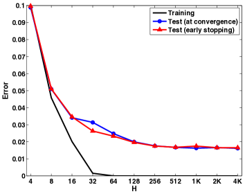
(a) MNIST

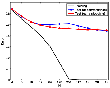
(b) CIFAR10

Figure 4.1: The training error and the test error based on different stopping criteria when 2-layer NNs with different number of hidden units are trained on MNIST and CIFAR-10. Images in both datasets are downsampled to 100 pixels. The size of the training set is 50000 for MNIST and 40000 for CIFAR-10. The early stopping is based on the error on a validation set (separate from the training and test sets) of size 10000. The training was done using stochastic gradient descent with momentum and mini-batches of size 100. The network was initialized with weights generated randomly from the Gaussian distribution. The initial step size and momentum were set to 0.1 and 0.5 respectively. After each epoch, we used the update rule $\mu^{(t+1)}=0.99\mu^{(t)}$ for the step size and $m^{(t+1)}=\min\{0.9,m^{(t)}+0.02\}$ for the momentum.

We also further tested this phenomena under some artificial mutilations to the data set. First, we wanted to artificially ensure that the approximation error was indeed zero and does not decrease as we add more units. To this end, we first trained a network with a small number $H_{0}$ of hidden units ($H_{0}=4$ on MNIST and $H_{0}=16$ on CIFAR) on the entire dataset (train+test+validation). This network did have some disagreements with the correct labels, but we then switched all labels to agree with the network creating a “censored” data set. We can think of this censored data as representing an artificial source distribution which can be exactly captured by a network with $H_{0}$ hidden units. That is, the approximation error is zero for networks with at least $H_{0}$ hidden units, and so does not decrease further. Still, as can be seen in the middle row of Figure he test error continues decreasing even after reaching zero training error.

Next, we tried to force overfitting by adding random label noise to the data. We wanted to see whether now the network will use its higher capacity to try to fit the noise, thus hurting generalization. However, as can be seen in the bottom row of Figure ven with five percent random labels, there is no significant overfitting and test error continues decreasing as network size increases past the size required for achieving zero training error.

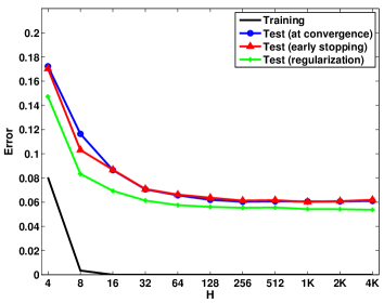
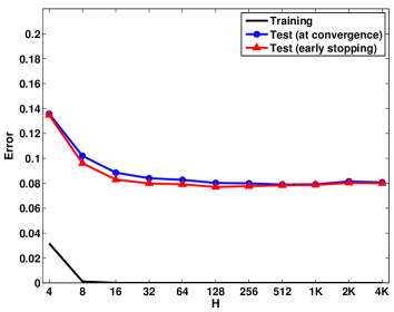
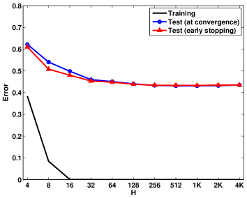
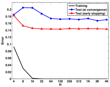
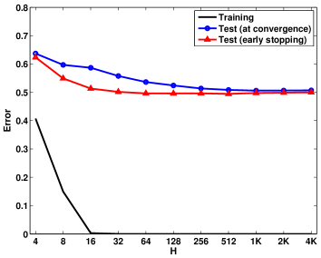
Figure 4.2: The training error and the test error based on different stopping criteria when 2-layer NNs with different number of hidden units are trained on small subsets of MNIST and CIFAR-10. Images in both datasets are downsampled to 100 pixels. The sizes of the training and validation sets are 2000 for both MNIST and CIFAR-10 and the early stopping is based on the error on the validation set. The top plots are the errors for the original datasets with and without explicit regularization.The best weight decay parameter is chosen based on the validation error. The middle plots are on the censored data set that is constructed by switching all the labels to agree with the predictions of a trained network with a small number $H_{0}$ of hidden units $H_{0}=4$ on MNIST and $H_{0}=16$ on CIFAR-10) on the entire dataset (train+test+validation). The plots on the bottom are also for the censored data except we also add 5 percent noise to the labels by randomly changing 5 percent of the labels. The optimization method is the same as the in Figure 1. The results in this figure are the average error over 5 random repetitions.

What is happening here? A possible explanation is that the optimization is introducing some implicit regularization. That is, we are implicitly trying to find a solution with small “complexity”, for some notion of complexity, perhaps norm. This can explain why we do not overfit even when the number of parameters is huge. Furthermore, increasing the number of units might allow for solutions that actually have lower “complexity”, and thus generalization better. Perhaps an ideal then would be an infinite network controlled only through this hidden complexity.

We want to emphasize that we are not including any explicit regularization, neither as an explicit penalty term nor by modifying optimization through, e.g., drop-outs, weight decay, or with one-pass stochastic methods. We are using a stochastic method, but we are running it to convergence—we achieve zero surrogate loss and zero training error. In fact, we also tried training using batch conjugate gradient descent and observed almost identical behavior. But it seems that even still, we are not getting to some random global minimum—indeed for large networks the vast majority of the many global minima of the training error would horribly overfit. Instead, the optimization is directing us toward a “low complexity” global minimum.

Although we do not know what this hidden notion of complexity is, as a final experiment we tried to see the effect of adding explicit regularization in the form of weight decay. The results are shown in the top row of figure here is a slight improvement in generalization but we still see that increasing the network size helps generalization.

4.2 A Matrix Factorization Analogy

To gain some understanding at what might be going on, let us consider a slightly simpler model which we do understand much better. Instead of rectified linear activations, consider a feed-forward network with a single hidden layer, and linear activations, i.e.:

$$f_{\mathbf{U},\mathbf{V}}(\mathbf{x})=\mathbf{U}\mathbf{V}\mathbf{x}$$ (4.2.1)

This is of course simply a matrix-factorization model, where $f_{\mathbf{W}}(\mathbf{x})=\mathbf{W}\mathbf{x}$ and $\mathbf{W}=\mathbf{V}\mathbf{U}$. Controlling capacity by limiting the number of hidden units exactly corresponds to constraining the rank of $\mathbf{W}$, i.e. biasing toward low dimensional factorizations. Such a low-rank inductive bias is indeed sensible, though computationally intractable to handle with most loss functions.

However, in the last decade we have seen much success for learning with low norm factorizations. In such models, we do not constrain the inner dimensionality $H$ of $\mathbf{U},\mathbf{V}$, and instead only constrain, or regularize, their norm. For example, constraining the Frobenius norm of $\mathbf{U}$ and $\mathbf{V}$ corresponds to using the trace-norm as an inductive bias [Srebro04]:

$$\left\lVert{\mathbf{W}}\right\rVert_{\text{tr}}=\min_{\mathbf{W}=\mathbf{V}\mathbf{U}}\frac{1}{2}(\left\lVert{\mathbf{U}}\right\rVert_{F}^{2}+\left\lVert{\mathbf{V}}\right\rVert_{F}^{2}).$$ (4.2.2)

Other norms of the factorization lead to different regularizers.

Unlike the rank, the trace-norm (as well as other factorization norms) is convex, and leads to tractable learning problems [Fazel01, Srebro04]. In fact, even if learning is done by a local search over the factor matrices $\mathbf{U}$ and $\mathbf{V}$ (i.e. by a local search over the weights of the network), if the dimensionality is high enough and the norm is regularized, we can ensure convergence to a global minima [Burer06]. This is in stark contrast to the dimensionality-constrained low-rank situation, where the limiting factor is the number of hidden units, and local minima are abundant [Srebro03].

Furthermore, the trace-norm and other factorization norms are well-justified as sensible inductive biases. We can ensure generalization based on having low trace-norm, and a low-trace norm model corresponds to a realistic factor model with many factors of limited overall influence. In fact, empirical evidence suggests that in many cases low-norm factorization are a more appropriate inductive bias compared to low-rank models.

We see, then, that in the case of linear activations (i.e. matrix factorization), the norm of the factorization is in a sense a better inductive bias than the number of weights: it ensures generalization, it is grounded in reality, and it explain why the models can be learned tractably.

Recently, gunasekar2017implicit provided empirical and theoretical evidence on the implicit regularization of gradient descent for matrix factorization. They showed that gradient descent on the full dimensional factorizations without any explicit regularization indeed converges to the minimum trace norm solution with initialization close enough to the origin and small enough step size.

Let us interpret the experimental results of Section this light. Perhaps learning is succeeding not because there is a good representation of the targets with a small number of units, but rather because there is a good representation with small overall norm, and the optimization is implicitly biasing us toward low-norm models. Such an inductive bias might potentially explain both the generalization ability and the computational tractability of learning, even using local search.

Under this interpretation, we really should be using infinite-sized networks, with an infinite number of hidden units. Fitting a finite network (with implicit regularization) can be viewed as an approximation to fitting the “true” infinite network. This situation is also common in matrix factorization: e.g., a very successful approach for training low trace-norm models, and other infinite-dimensional bounded-norm factorization models, is to approximate them using a finite dimensional representation [rennie2005fast, srebro2010collaborative]. The finite dimensionality is then not used at all for capacity (statistical complexity) control, but purely for computational reasons. Indeed, increasing the allowed dimensionality generally improves generalization performance, as it allows us to better approximate the true infinite model. Inspired by these experiments, in order to understand the implicit regularization in deep learning, we will next look at ways of controlling the capacity independent of the number of hidden units.

Chapter 5 Norm-based Capacity Control

As we discussed in Section atistical complexity, or capacity, of unregularized feed-forward neural networks, as a function of the network size and depth, is fairly well understood. But feedforward networks are often trained with some kind of regularization, such as weight decay, early stopping, “max regularization”, or more exotic regularization such as drop-outs. We also showed in Chapter at even without any explicit regularization, the capacity of neural networks is being controlled by a form of implicit regularization caused by optimization which does not depend on the size of the network. What is the effect of such regularization on the induced model class and its capacity?

For linear prediction (a one-layer feed-forward network) we know that using regularization the capacity of the class can be bounded only in terms of the norms, with no (or a very weak) dependence on the number of edges (i.e. the input dimensionality or number of linear coefficients). E.g., we understand very well how the capacity of $\ell_{2}$-regularized linear predictors can be bounded in terms of the norm alone (when the norm of the data is also bounded), even in infinite dimension.

A central question we ask is: can we bound the capacity of feed-forward network in terms of norm-based regularization alone, without relying on network size and even if the network size (number of nodes or edges) is unbounded or infinite? What type of regularizers admit such capacity control? And how does the capacity behave as a function of the norm, and perhaps other network parameters such as depth?

Beyond the central question of capacity control, we also analyze the convexity of the resulting model class—unlike unregularized size-controlled feed-forward networks, infinite magnitude-controlled networks have the potential of yielding convex model classes (this is the case, e.g., when we move from rank-based control on matrices, which limits the number of parameters to magnitude based control with the trace-norm or max-norm). A convex class might be easier to optimize over and might be convenient in other ways.

In this chapter we focus on two natural types of norm regularization: bounding the norm of the incoming weights of each unit (per-unit regularization) and bounding the overall norm of all the weights in the system jointly (overall regularization, e.g. limiting the overall sum of the magnitudes, or square magnitudes, in the system). We generalize both of these with a single notion of group-norm regularization: we take the $\ell_{p}$ norm over the weights in each unit and then the $\ell_{q}$ norm over units. In Section present this regularizer and obtain a tight understanding of when it provides for size-independent capacity control and a characterization of when it induces convexity. We then apply these generic results to per-unit regularization (Section nd overall regularization (Section noting also other forms of regularization that are equivalent to these two. In particular, we show how per-unit regularization is equivalent to a novel path-based regularizer and how overall $\ell_{2}$ regularization for two-layer networks is equivalent to so-called “convex neural networks” [Bengio05]. In terms of capacity control, we show that per-unit regularization allows size-independent capacity-control only with a per-unit $\ell_{1}$-norm, and that overall $\ell_{p}$ regularization allows for size-independent capacity control only when $p\leq 2$, even if the depth is bounded. In any case, even if we bound the sum of all magnitudes in the system, we show that an exponential dependence on the depth is unavoidable.

As far as we are aware, prior work on size-independent capacity control for feed-forward networks considered only per-unit $\ell_{1}$ regularization, and per-unit $\ell_{2}$ regularization for two-layered networks (see discussion and references at the beginning of Section Recently, bartlett2017spectrally have shown a generalization bound based on the product of spectral norm of the layers using covering numbers. In Chapter e show a simpler prove for a tighter bound. Here, we extend the scope significantly, and provide a broad characterization of the types of regularization possible and their properties. In particular, we consider overall norm regularization, which is perhaps the most natural form of regularization used in practice (e.g. in the form of weight decay). We hope our study will be useful in thinking about, analyzing and designing learning methods using feed-forward networks. Another motivation for us is that complexity of large-scale optimization is often related to scale-based, not dimension-based complexity. Understanding when the scale-based complexity depends exponentially on the depth of a network might help shed light on understanding the difficulties in optimizing deep networks.

Preliminaries and Notations

We denote by $\mathcal{F}^{d,H}$ the class of fully connected feedforward networks with a single output node and use the shorthand $\mathcal{F}^{d}=\mathcal{F}^{d,\infty}$. We will consider various measures $\mu(\mathbf{w})$ of the magnitude of the weights $\mathbf{w}$. Such a measure induces a complexity measure on functions $f\in\mathcal{F}^{d,H}$ defined by $\mu^{d,H}(f)=\inf_{f_{\mathbf{w}}=f}\mu(\mathbf{w})$. The sublevel sets of the complexity measure $\mu^{d,H}$ form a family of hypothesis classes $\mathcal{F}^{d,H}_{\mu\leq a}=\{f\in\mathcal{F}^{d,H}\;|\;\mu^{d,H}(f)\leq a\}$.

For binary function $g:\{\pm 1\}^{n_{\text{in}}}\rightarrow{\pm 1}$ we say that $g$ is realized by $f$ with unit margin if $\forall_{x}f(x)g(x)\geq 1$. A set of points $\mathcal{S}_{\text{in}}$ is shattered with unit margin by a model class $\mathcal{F}$ if all $g:\mathcal{S}_{\text{in}}\rightarrow{\pm 1}$ can be realized with unit margin by some $f_{\mathbf{w}}\in\mathcal{F}$.

5.1 Group Norm Regularization

Considering the grouping of weights going into each edge of the network, we will consider the following generic group-norm type regularizer, parametrized by $1\leq p,q\leq\infty$:

$$\mu_{p,q}(\mathbf{w})=\left(\sum_{v\in V}\left(\sum_{(u\rightarrow v)\in E}\left\lvert w_{u\rightarrow v}\right\rvert^{p}\right)^{q/p}\right)^{1/q}.$$ (5.1.1)

Here and elsewhere we allow $q=\infty$ with the usual conventions that $(\sum z_{i}^{q})^{1/q}=\sup z_{i}$ and $1/q=0$ when it appears in other contexts. When $q=\infty$ the group regularizer (5.1.1) imposes a per-unit regularization, where we constrain the norm of the incoming weights of each unit separately, and when $q=p$ the regularizer (5.1.1) is an “overall” weight regularizer, constraining the overall norm of all weights in the system. E.g., when $q=p=1$ we are paying for the sum of all magnitudes of weights in the network, and $q=p=2$ corresponds to overall weight-decay where we pay for the sum of square magnitudes of all weights (i.e. the overall Euclidean norm of the weights).

For a layered graph, we have:

$$\mu_{p,q}(\mathbf{w}) =\left(\sum_{k=1}^{d}\sum_{i=1}^{H}\left(\sum_{j=1}^{H}{\left\lvert{W^{k}[i,j]}\right\rvert}^{p}\right)^{q/p}\right)^{1/q}\!\!=d^{1/q}\left(\frac{1}{d}\sum_{k=1}^{d}\left\lVert{W^{k}}\right\rVert^{q}_{p,q}\right)^{1/q}$$

$$\geq d^{1/q}\left(\prod_{k=1}^{d}\left\lVert{W^{k}}\right\rVert_{p,q}\right)^{1/d}\stackrel{{\scriptstyle\text{def}}}{{=}}d^{1/q}\sqrt[d]{\psi_{p,q}(\mathbf{w})}$$ (5.1.2)

where $\displaystyle\psi_{p,q}(\mathbf{w})=\prod_{k=1}^{d}\left\lVert{W^{k}}\right\rVert_{p,q}$ aggregates the layers by multiplication instead of summation. The inequality (5.1.2) holds regardless of the activation function, and so for any $\sigma$ we have:

$$\psi_{p,q}^{d,H}(f)\leq\left(\frac{\mu^{d,H}(f)_{p,q}}{d^{1/q}}\right)^{d}.$$ (5.1.3)

But due to the homogeneity of the RELU activation, when this activation is used we can always balance the norm between the different layers without changing the computed function so as to achieve equality in (5.1.2):

Claim 2.

For any $f_{\mathbf{w}}\in\mathcal{F}^{d,H}$, $\displaystyle\mu^{d,H}_{p,q}(f)=d^{1/q}\sqrt[d]{\psi_{p,q}^{d,H}(f)}$.

Proof.

Let $\mathbf{w}$ be weights that realizes $f$ and are optimal with respect to $\psi_{p,g}$; i.e. $\psi_{p,q}(\mathbf{w})=\psi^{d,H}_{p,q}(\mathbf{w})$. Let $\widetilde{W}^{k}=\sqrt[d]{\psi_{p,q}(\mathbf{w})}W^{k}/\left\lVert{W^{k}}\right\rVert_{p,q}$, and observe that they also realize $f$. We now have:

$$\mu^{d,H}_{p,q}(f)\leq\mu_{p,q}(\widetilde{W})=\Bigl{(}\sum\nolimits_{k=1}^{d}\left\lVert{\widetilde{W}^{k}}\right\rVert^{q}_{p,q}\Bigr{)}^{1/q}=\Bigl{(}d\Bigl{(}\psi_{p,q}(\mathbf{w})\Bigr{)}^{q/d}\Bigr{)}^{1/q}=d^{1/q}\sqrt[d]{\psi^{d,H}_{p,q}(f)}$$

which together with (5.1.2) completes the proof. ∎

The two measures are therefore equivalent when we use RELUs, and define the same level sets, or family of model classes, which we refer to simply as $\mathcal{F}^{d,H}_{p,q}$. In the remainder of this Section, we investigate convexity and generalization properties of these model classes.

5.1.1 Generalization and Capacity

In order to understand the effect of the norm on the sample complexity, we bound the Rademacher complexity of the classes $\mathcal{F}^{d,H}_{p,q}$. Recall that the Rademacher Complexity is a measure of the capacity of a model class on a specific sample, which can be used to bound the difference between empirical and expected error, and thus the excess generalization error of empirical risk minimization (see, e.g., [bartlett03] for a complete treatment, and Section r the exact definitions we use). In particular, the Rademacher complexity typically scales as $\sqrt{C/m}$, which corresponds to a sample complexity of $O(C/\epsilon^{2})$, where $m$ is the sample size and $C$ is the effective measure of capacity of the model class.

Theorem 3.

For any $d,q\geq 1$, any $1\leq p<\infty$ and any set $\mathcal{S}=\{x_{1},\dots,x_{m}\}\subseteq\mathbb{R}^{n_{\text{in}}}$:

$$\mathcal{R}_{m}(\mathcal{F}_{\psi_{p,q}\leq\psi}^{d,H}) \leq\psi\left(2H^{[\frac{1}{p^{*}}-\frac{1}{q}]_{+}}\right)^{(d-1)}\mathcal{R}^{\text{linear}}_{m,p,n_{\text{in}}}$$

$$\leq\sqrt{\frac{\psi^{2}\left(2H^{[\frac{1}{p^{*}}-\frac{1}{q}]_{+}}\right)^{2(d-1)}\min\{p^{*},4\log(2n_{\text{in}})\}\max_{i}\left\lVert{x_{i}}\right\rVert_{p^{*}}^{2}}{m}}$$

and so:

$$\mathcal{R}_{m}(\mathcal{F}_{\mu_{p,q}\leq\mu}^{d,H}) \leq\mu^{d}\left(2H^{[\frac{1}{p^{*}}-\frac{1}{q}]_{+}}/\sqrt[q]{d}\right)^{(d-1)}\mathcal{R}^{\text{linear}}_{m,p,n_{\text{in}}}$$

$$\leq\sqrt{\frac{\mu^{2d}\left(2H^{[\frac{1}{p^{*}}-\frac{1}{q}]_{+}}/\sqrt[q]{d}\right)^{2(d-1)}\min\{p^{*},4\log(2n_{\text{in}})\}\max_{i}\left\lVert{x_{i}}\right\rVert_{p^{*}}^{2}}{m}}$$

where the second inequalities hold only if $1\leq p\leq 2$, $\mathcal{R}^{\text{linear}}_{m,p,n_{\text{in}}}$ is the Rademacher complexity of $n_{\text{in}}$-dimensional linear predictors with unit $\ell_{p}$ norm with respect to a set of $m$ samples and $p^{*}$ is such that $\frac{1}{p^{*}}+\frac{1}{p}=1$.

Proof sketch

We prove the bound by induction, showing that for any $q,d>1$ and $1\leq p<\infty$,

$$\mathcal{R}_{m}(\mathcal{F}_{\psi_{p,q}\leq\psi}^{d,H})\leq 2H^{[\frac{1}{p^{*}}-\frac{1}{q}]_{+}}\mathcal{R}_{m}(\mathcal{F}_{\psi_{p,q}\leq\psi}^{d-1,H}).$$

The intuition is that when $p^{*}<q$, the Rademacher complexity increases by simply distributing the weights among neurons and if $p^{*}\geq q$ then the supremum is attained when the output neuron is connected to a neuron with highest Rademacher complexity in the lower layer and all other weights in the top layer are set to zero. For a complete proof, see Section sketch

Note that for $2\leq p<\infty$, the bound on the Rademacher complexity scales with $m^{\frac{1}{p}}$ (see Section ecause:

$$\mathcal{R}^{\text{linear}}_{m,p,n_{\text{in}}}\leq\frac{\sqrt{2}\left\lVert{X}\right\rVert_{2,p^{*}}}{m}\leq\frac{\sqrt{2}\max_{i}\left\lVert{x_{i}}\right\rVert_{p^{*}}}{m^{\frac{1}{p}}}$$ (5.1.4)

The bound in Theorem pends on both the magnitude of the weights, as captured by $\mu_{p,q}(\mathbf{w})$ or $\psi_{p,q}(\mathbf{w})$, and also on the width $H$ of the network (the number of nodes in each layer). However, the dependence on the width $H$ disappears, and the bound depends only on the magnitude, as long as $q\leq p^{*}$ (i.e. $1/p+1/q\geq 1$). This happens, e.g., for overall $\ell_{1}$ and $\ell_{2}$ regularization, for per-unit $\ell_{1}$ regularization, and whenever $1/p+1/q=1$. In such cases, we can omit the size constraint and state the theorem for an infinite-width layered network (i.e. a network with an infinitely countable number of units, when the number of units is allowed to be as large as needed):

Corollary 4.

For any $d\geq 1$, $1\leq p<\infty$ and $1\leq q\leq p^{*}=p/(p-1)$, and any set $\mathcal{S}=\{x_{1},\dots,x_{m}\}\subseteq\mathbb{R}^{n_{\text{in}}}$,

$$\mathcal{R}_{m}(\mathcal{F}_{\psi_{p,q}\leq\psi}^{d,H}) \leq\psi 2^{(d-1)}\mathcal{R}^{\text{linear}}_{m,p,n_{\text{in}}}$$

$$\leq\sqrt{\frac{\psi^{2}\left(2H^{[\frac{1}{p^{*}}-\frac{1}{q}]_{+}}\right)^{2(d-1)}\min\{p^{*},4\log(2n_{\text{in}})\}\max_{i}\left\lVert{x_{i}}\right\rVert_{p^{*}}^{2}}{m}}$$

and so:

$$\mathcal{R}_{m}(\mathcal{F}_{\mu_{p,q}\leq\mu}^{d,H}) \leq\left(2\mu/\sqrt[q]{d}\right)^{d}\mathcal{R}^{\text{linear}}_{m,p,n_{\text{in}}}$$

$$\leq\sqrt{\frac{\left(2\mu/\sqrt[q]{d}\right)^{2d}\min\{p^{*},4\log(2n_{\text{in}})\}\max_{i}\left\lVert{x_{i}}\right\rVert_{p^{*}}^{2}}{m}}$$

where the second inequalities hold only if $1\leq p\leq 2$ and $\mathcal{R}^{\text{linear}}_{m,p,n_{\text{in}}}$ is the Rademacher complexity of $n_{\text{in}}$-dimensional linear predictors with unit $\ell_{p}$ norm with respect to a set of $m$ samples.

5.1.2 Tightness

We next investigate the tightness of the complexity bound in Theorem nd show that when $1/p+1/q<1$ the dependence on the width $H$ is indeed unavoidable. We show not only that the bound on the Rademacher complexity is tight, but that the implied bound on the sample complexity is tight, even for binary classification with a margin over binary inputs. To do this, we show how we can shatter the $m=2^{n_{\text{in}}}$ points $\{\pm 1\}^{n_{\text{in}}}$ using a network with small group-norm:

Theorem 5.

For any $p,q\geq 1$ (and $1/p^{*}+1/p=1$) and any depth $d\geq 2$, the $m=2^{n_{\text{in}}}$ points $\{\pm 1\}^{n_{\text{in}}}$ can be shattered with unit margin by $\mathcal{F}^{d,H}_{\psi_{p,q}\leq\psi}$ with:

$$\psi\leq n_{\text{in}}^{1/p}\,m^{1/p+1/q}\,H^{-(d-2)[1/p^{*}-1/q]_{+}}$$

Proof.

Consider a size $m$ subset $S_{m}$ of $2^{n_{\text{in}}}$ vertices of the $n_{\text{in}}$ dimensional hypercube $\{-1,+1\}^{n_{\text{in}}}$. We construct the first layer using $m$ units. Each unit has a unique weight vector consisting of $+1$ and $-1$’s and will output a positive value if and only if the sign pattern of the input $x\in\mathcal{S}_{m}$ matches that of the weight vector. The second layer has a single unit and connects to all $m$ units in the first layer. For any $m$ dimensional sign pattern $b\in\{-1,+1\}^{m}$, we can choose the weights of the second layer to be $b$, and the network will output the desired sign for each $x\in\mathcal{S}_{m}$ with unit margin. The norm of the network is at most $(m\cdot n_{\text{in}}^{q/p})^{1/q}\cdot m^{1/p}=n_{\text{in}}^{1/p}\cdot m^{(1/p+1/q)}.$ This establishes the claim for $d=2$. For $d>2$ and $1/p+1/q\geq 1$, we obtain the same norm and unit margin by adding $d-2$ layers with one unit in each layer connected to the previous layer by a unit weight. For $d>2$ and $1/p+1/q<1$, we show the dependence on $H$ by recursively replacing the top unit with $H$ copies of it and adding an averaging unit on top of that. More specifically, given the above $d=2$ layer network, we make $H$ copies of the output unit with rectified linear activation and add a 3rd layer with one output unit with uniform weight $1/H$ to all the copies in the 2nd layer. Since this operation does not change the output of the network, we have the same margin and now the norm of the network is $(m\cdot n_{\text{in}}^{q/p})^{1/q}\cdot(Hm^{q/p})^{1/q}\cdot(H(1/H^{p}))^{1/p}=n_{\text{in}}^{1/p}\cdot m^{(1/p+1/q)}\cdot H^{1/q-1/p^{*}}.$ That is, we have reduced the norm by factor $H^{1/q-1/p^{*}}$. By repeating this process, we get the geometric reduction in the norm $H^{(d-2)(1/q-1/p^{*})}$, which concludes the proof. ∎

To understand this lower bound, first consider the bound without the dependence on the width $H$. We have that for any depth $d\geq 2$, $\psi\leq m^{r}n_{\text{in}}=m^{r}\log m$ (since $1/p\leq 1$ always) where $r=1/p+1/q\leq 2$. This means that for any depth $d\geq 2$ and any $p,q$ the sample complexity of learning the class scales as $m=\Omega(\psi^{1/r}/\log\psi)\geq\tilde{\Omega}(\sqrt{\psi})$. This shows a polynomial dependence on $\psi$, though with a lower exponent than the $\psi^{2}$ (or higher for $p>2$) dependence in Theorem till, if we now consider the complexity control as a function of $\mu_{p,q}$ we get a sample complexity of at least $\Omega(\mu^{d/2}/\log\mu)$, establishing that if we control the group-norm as in (5.1.1), we cannot avoid a sample complexity which depends exponentially on the depth. Note that in our construction, all other factors in Theorem amely $\max_{i}\left\lVert{x_{i}}\right\rVert$ and $\log n_{\text{in}}$, are logarithmic (or double-logarithmic) in $m$.

Next we consider the dependence on the width $H$ when $1/p+1/q<1$. Here we have to use depth $d\geq 3$, and we see that indeed as the width $H$ and depth $d$ increase, the magnitude control $\psi$ can decrease as $H^{(1/p^{*}-1/q)(d-2)}$ without decreasing the capacity, matching Theorem 1 up to an offset of 2 on the depth. In particular, we see that in this regime we can shatter an arbitrarily large number of points with arbitrarily low $\psi$ by using enough hidden units, and so the capacity of $\mathcal{F}^{d}_{p,q}$ is indeed infinite and it cannot ensure any generalization.

5.1.3 Convexity

Finally we establish a sufficient condition for the model classes $\mathcal{F}^{d}_{p,q}$ to be convex. We are referring to convexity of the functions in the $\mathcal{F}^{d}_{p,q}$ independent of a specific representation. If we consider a, possibly regularized, empirical risk minimization problem on the weights, the objective (the empirical risk) would never be a convex function of the weights (for depth $d\geq 2$), even if the regularizer is convex in $w$ (which it always is for $p,q\geq 1$). But if we do not bound the width of the network, and instead rely on magnitude-control alone, we will see that the resulting model class, and indeed the complexity measure, may be convex (with respect to taking convex combinations of functions, not of weights).

Theorem 6.

For any $d,p,q\geq 1$ such that $\frac{1}{q}\leq\frac{1}{d-1}\big{(}1-\frac{1}{p}\big{)}$, $\psi^{d}_{p,q}(f)$ is a semi-norm in $\mathcal{F}^{d}$.

In particular, under the condition of the Theorem, $\psi^{d}_{p,q}$ is convex, and hence its sublevel sets $\mathcal{F}^{d}_{p,q}$ are convex, and so $\mu^{d}_{p,q}$ is quasi-convex (but not convex).

Proof sketch

To show convexity, consider two functions $f,g\in\mathcal{F}^{d}_{\psi_{p,q}\leq\psi}$ and $0<\alpha<1$, and let $U$ and $V$ be the weights realizing $f$ and $g$ respectively with $\psi_{p,q}(U)\leq\psi$ and $\psi_{p,q}(V)\leq\psi$. We will construct weights $\mathbf{w}$ realizing $\alpha f+(1-\alpha)g$ with $\psi_{p,q}(\mathbf{w})\leq\psi$. This is done by first balancing $U$ and $V$ s.t. at each layer $\left\lVert{U_{i}}\right\rVert_{p,q}=\sqrt[d]{\psi_{p,q}(U)}$ and $\left\lVert{V_{i}}\right\rVert_{p,q}=\sqrt[d]{\psi_{p,q,}(V)}$ and then placing $U$ and $V$ side by side, with no interaction between the units calculating $f$ and $g$ until the output layer. The output unit has weights $\alpha U_{d}$ coming in from the $f$-side and weights $(1-\alpha)V_{d}$ coming in from the $g$-side. In Section show that under the condition in the theorem, $\psi_{p,q}(\mathbf{w})\leq\psi$. To complete the proof, we also show $\psi^{d}_{p,q}$ is homogeneous and that this is sufficient for convexity. $\blacksquare$

5.2 Per-Unit and Path Regularization

In this Section we will focus on the special case of $q=\infty$, i.e. when we constrain the norm of the incoming weights of each unit separately.

Per-unit $\ell_{1}$-regularization was studied by [bartlett98, koltchinskii02, bartlett03] who showed generalization guarantees. A two-layer network of this form with RELU activation was also considered by [Bach14], who studied its approximation ability and suggested heuristics for learning it. Per-unit $\ell_{2}$ regularization in a two-layer network was considered by [Cho09], who showed it is equivalent to using a specific kernel. We now introduce Path regularization and discuss its equivalence to Per-Unit regularization.

Path Regularization

Consider a regularizer which looks at the sum over all paths from input nodes to the output node, of the product of the weights along the path:

$$\phi_{p}(\mathbf{w})=\Bigl{(}\sum_{v_{\textrm{in}}[i]\overset{e_{1}}{\rightarrow}v_{1}\overset{e_{2}}{\rightarrow}v_{2}\cdots\overset{e_{k}}{\rightarrow}v_{\textrm{out}}}\prod_{i=1}^{k}{\left\lvert{w_{e_{i}}}\right\rvert}^{p}\Bigr{)}^{1/p}$$ (5.2.1)

where $p\geq 1$ controls the norm used to aggregate the paths. We can motivate this regularizer as follows: if a node does not have any high-weight paths going out of it, we really don’t care much about what comes into it, as it won’t have much effect on the output. The path-regularizer thus looks at the aggregated influence of all the weights.

Referring to the induced regularizer $\phi^{G}_{p}(f)=\min_{f_{\mathbf{w}}=f}\phi_{p}(\mathbf{w})$ (with the usual shorthands for layered graphs), we now observe that for layered graphs, path regularization and per-unit regularization are equivalent:

Theorem 7.

For $p\geq 1$, any $d$ and (finite or infinite) $H$, for any $f_{\mathbf{w}}\in\mathcal{F}^{d,H}$: $\phi_{p}^{d,H}(f)=\psi^{d,H}_{p,\infty}$

It is important to emphasize that even for layered graphs, it is not the case that for all weights $\phi_{p}(\mathbf{w})=\psi_{p,\infty}(\mathbf{w})$. E.g., a high-magnitude edge going into a unit with no non-zero outgoing edges will affect $\psi_{p,\infty}(\mathbf{w})$ but not $\phi_{p}(\mathbf{w})$, as will having high-magnitude edges on different layers in different paths. In a sense path regularization is as more careful regularizer less fooled by imbalance. Nevertheless, in the proof of Theorem Section e show we can always balance the weights such that the two measures are equal.

The equivalence does not extend to non-layered graphs, since the lengths of different paths might be different. Again, we can think of path regularizer as more refined regularizer taking into account the local structure. However, if we consider all DAGs of depth at most $d$ (i.e. with paths of length at most $d$), the notions are again equivalent (see proof in Section theorem For any $p≥1$ and any $d$: $ψ^d_p,∞(f) = min_$G∈DAG(d)$ ϕ^G_p(f)$.

In particular, for any graph $G$ of depth $d$, we have that $\phi^{G}_{p}(f)\geq\psi^{d}_{p,\infty}(f)$. Combining this observation with Corollary lows us to immediately obtain a generalization bound for path regularization on any, even non-layered, graph:

Corollary 8.

For any graph $G$ of depth $d$ and any set $\mathcal{S}=\{x_{1},\dots,x_{m}\}\subseteq\mathbb{R}^{n_{\text{in}}}$:

$$\mathcal{R}_{m}(\mathcal{F}^{G}_{\phi_{1}\leq\phi})\leq\sqrt{\frac{4^{d-1}\phi^{2}\cdot 4\log(2n_{\text{in}})\sup\left\lVert{x_{i}}\right\rVert_{\infty}^{2}}{m}}$$

Note that in order to apply Corollary d obtain a width-independent bound, we had to limit ourselves to $p=1$. We further explore this issue next.

Capacity

As was previously noted, size-independent generalization bounds for bounded depth networks with bounded per-unit $\ell_{1}$ norm have long been known (and make for a popular homework problem). These correspond to a specialization of Corollary r the case $p=1,q=\infty$. Furthermore, the kernel view of [Cho09] allows obtaining size-independent generalization bound for two-layer networks with bounded per-unit $\ell_{2}$ norm (i.e. a single infinite hidden layer of all possible unit-norm units, and a bounded $\ell_{2}$-norm output unit). However, the lower bound of Theorem tablishes that for any $p>1$, once we go beyond two layers, we cannot ensure generalization without also controlling the size (or width) of the network.

Convexity

An immediately consequence of Theorem that per-unit regularization, if we do not constrain the network width, is convex for any $p\geq 1$. In fact, $\psi^{d}_{p,\infty}$ is a (semi)norm. However, as discussed above, for depth $d>2$ this is meaningful only for $p=1$, as $\psi^{d}_{p,\infty}$ collapses for $p>1$.

Hardness

Since the classes $\mathcal{F}^{d}_{1,\infty}$ are convex, we might hope that this might make learning computationally easier. Indeed, one can consider functional-gradient or boosting-type strategies for learning a predictor in the class [lee96]. However, as Bach14 points out, this is not so easy as it requires finding the best fit for a target with a RELU unit, which is not easy. Indeed, applying results on hardness of learning intersections of halfspaces, which can be represented with small per-unit norm using two-layer networks, we can conclude that, subject to certain complexity assumptions, it is not possible to efficiently PAC learn $\mathcal{F}^{d}_{1,\infty}$, even for depth $d=2$ when $\psi_{1,\infty}$ increases superlinearly:

Corollary 9.

Subject to the the strong random CSP assumptions in [Daniely14], it is not possible to efficiently PAC learn (even improperly) functions $\{\pm 1\}^{n_{\text{in}}}\rightarrow\{\pm 1\}$ realizable with unit margin by $\mathcal{F}^{2}_{1,\infty}$ when $\psi_{1,\infty}=\omega(n_{\text{in}})$ (e.g. when $\psi_{1,\infty}=n_{\text{in}}\log n_{\text{in}}$). Moreover, subject to intractability of $\tilde{Q}(n_{\text{in}}^{1.5})$-unique shortest vector problem, for any $\epsilon>0$, it is not possible to efficiently PAC learn (even improperly) functions $\{\pm 1\}^{n_{\text{in}}}\rightarrow\{\pm 1\}$ realizable with unit margin by $\mathcal{F}^{2}_{1,\infty}$ when $\psi_{1,\infty}=n_{\text{in}}^{1+\epsilon}$.

This is a corollary of Theorem the Section ither versions of corollary ecludes the possibility of learning in time polynomial in $\psi_{1,\infty}$, though it still might be possible to learn in $\textrm{poly}(n_{\text{in}})$ time when $\psi_{1,\infty}$ is sublinear.

Sharing

We conclude this Section with an observation on the type of networks obtained by per-unit, or equivalently path, regularization.

Theorem 10.

For any $p\geq 1$ and $d>1$ and any $f_{\mathbf{w}}\in\mathcal{F}^{d}$, there exists a layered graph $G(V,E)$ of depth $d$, such that $f_{\mathbf{w}}\in\mathcal{F}^{G}$ and $\psi^{G}_{p,\infty}(f)=\phi^{G}_{p}(f)=\psi^{d}_{p,\infty}(f)$, and the out-degree of every internal (non-input) node in $G$ is one. That is, the subgraph of $G$ induced by the non-input vertices is a tree directed toward the output vertex.

What the Theorem tells us is that we can realize every function as a tree with optimal per-unit norm. If we think of learning with an infinite fully-connected layered network, we can always restrict ourselves to models in which the non-zero-weight edges form a tree. This means that when using per-unit regularization we have no incentive to “share” lower-level units—each unit will only have a single outgoing edge and will only be used by a single down-stream unit. This seems to defy much of the intuition and power of using deep networks, where we expect lower layers to represent generic feature useful in many higher-level features. In effect, we are not encouraging any transfer between learning different aspects of the function (or between different tasks or classes, if we do have multiple output units). Per-unit regularization therefore misses out on much of the inductive bias that we might like to impose when using deep learning (namely, promoting sharing).

Proof.

[of Theorem For any $f_{\mathbf{w}}\in\mathcal{F}^{\text{DAG}(d)}$, we show how to construct such $\widetilde{G}$ and $\widetilde{w}$. We first sort the vertices of $G$ based on topological ordering such that the out-degree of the first vertex is zero. Let $G_{0}=G$ and $w_{0}=w$. At each step $i$, we first set $G_{i}=G_{i-1}$ and $w_{i}=w_{i-1}$ and then pick the vertex $u$ that is the $i$th vector in the topological ordering. If the out-degree of $u$ is at most 1. Otherwise, for any edge $(u\rightarrow v)$ we create a copy of vertex $u$ that we call it $u_{v}$, add the edge $(u_{v}\rightarrow v)$ to $G_{i}$ and connect all incoming edges of $u$ with the same weights to every such $u_{v}$ and finally we delete the vertex $u$ from $G_{i}$ together with all incoming and outgoing edges of $u$. It is easy to indicate that $f_{G_{i},w_{i}}=f_{G_{i-1},w_{i-1}}$. After at most $|V|$ such steps, all internal nodes have out-degree one and hence the subgraph induced by non-input vertices will be a tree. ∎

5.3 Overall Regularization

In this Section, we will focus on “overall” $\ell_{p}$ regularization, corresponding to the choice $q=p$, i.e. when we bound the overall (vectorized) norm of all weights in the system:

$$\mu_{p,p}(\mathbf{w})=\Bigl{(}\sum_{e\in E}{\left\lvert{w(e)}\right\rvert}^{p}\Bigr{)}^{1/p}.$$

Capacity

For $p\leq 2$, Corollary ovides a generalization guarantee that is independence of the width—we can conclude that if we use weight decay (overall $\ell_{2}$ regularization), or any tighter $\ell_{p}$ regularization, there is no need to limit ourselves to networks of finite size (as long as the corresponding dual-norm of the inputs are bounded). However, in Section saw that with $d\geq 3$ layers, the regularizer degenerates and leads to infinite capacity classes if $p>2$. In any case, even if we bound the overall $\ell_{1}$-norm, the complexity increases exponentially with the depth.

Convexity

The conditions of Theorem r convexity of $\mathcal{F}^{d}_{2,2}$ are ensured when $p\geq d$. For depth $d=1$, i.e. a single unit, this just confirms that $\ell_{p}$-regularized linear prediction is convex for $p\geq 1$. For depth $d=2$, we get convexity with $\ell_{2}$ regularization, but not $\ell_{1}$. For depth $d>2$ we would need $p>d\geq 3$, however for such values of $p$ we know from Theorem at $\mathcal{F}^{d}_{p,p}$ degenerates to an infinite capacity class if we do not control the width (if we do control the width, we do not get convexity). This leaves us with $\mathcal{F}^{2}_{2,2}$ as the interesting convex class. Below we show an explicit convex characterization of $\mathcal{F}^{2}_{2,2}$ by showing it is equivalent to so-called “convex neural nets”.

Convex Neural Nets [Bengio05] over inputs in $\mathbb{R}^{n_{\text{in}}}$ are two-layer networks with a fixed infinite hidden layer consisting of all units with weights $w\in\mathcal{G}$ for some base class $\mathcal{G}\in\mathbb{R}^{n_{\text{in}}}$, and a second $\ell_{1}$-regularized layer. Since over finite data the weights in the second layer can always be taken to have finite support (i.e. be non-zero for only a finite number of first-layer units), and we can approach any function with countable support, we can instead think of a network in $\mathcal{F}^{2}$ where the bottom layer is constraint to $\mathcal{G}$ and the top layer is $\ell_{1}$ regularized. Focusing on $\mathcal{G}=\{w\,|\,\left\lVert{w}\right\rVert_{p}\leq 1\}$, this corresponds to imposing an $\ell_{p}$ constraint on the bottom layer, and $\ell_{1}$ regularization on the top layer and yields the following complexity measure over $\mathcal{F}^{2}$:

$$\nu_{p}(f)=\inf_{f_{\text{layer}(d),W}=f,\textrm{s.t.}\forall_{j}\left\lVert{W_{1}[j,:]}\right\rVert_{p}\leq 1}\left\lVert{W_{2}}\right\rVert_{1}.$$ (5.3.1)

This is similar to per-unit regularization, except we impose different norms at different layers (if $p\not=1$). We can see that $\mathcal{F}^{2}_{\nu_{p}\leq\nu}=\nu\cdot\overline{\operatorname{conv}}(\sigma(\mathcal{G}))$, and is thus convex for any $p$. Focusing on RELU activation we have the equivalence:

Theorem 11.

$\displaystyle\mu^{2}_{2,2}(f)=2\nu_{2}(f).$

That is, overall $\ell_{2}$ regularization with two layers is equivalent to a convex neural net with $\ell_{2}$-constrained units on the bottom layer and $\ell_{1}$ (not $\ell_{2}$!) regularization on the output.

Proof.

We can calculate:

$$\min_{f_{W}=f}\mu_{2,2}^{2}(\mathbf{w}) =\min_{f_{W}=f}\sum_{j=1}^{H}\left(\sum_{i=1}^{n_{\text{in}}}|W_{1}[j,i]|^{2}+|W_{2}[j]|^{2}\right)$$

$$=\min_{f_{W}=f}\sum_{j=1}^{H}2\sqrt{\sum\nolimits_{i=1}^{n_{\text{in}}}|W_{1}[j,i]|^{2}}\cdot|W_{2}[j]|$$ (5.3.2)

$$=2\min_{f_{W}=f}\sum_{j=1}^{H}\left|W_{2}[j]\right|\quad\text{s.t.}\quad\sqrt{\sum\nolimits_{i=1}^{n_{\text{in}}}|W_{1}[j,i]|^{2}}\leq 1.$$ (5.3.3)

Here (5.3.2) is the arithmetic-geometric mean inequality for which we can achieve equality by balancing the weights (as in Claim nd (5.3.3) again follows from the homogeneity of the RELU which allows us to rebalance the weights. ∎

Hardness

As with $\mathcal{F}^{d}_{1,\infty}$, we might hope that the convexity of $\mathcal{F}^{2}_{2,2}$ might make it computationally easy to learn. However, by the same reduction from learning intersection of halfspaces (Theorem Section e can again conclude that we cannot learn in time polynomial in $\mu^{2}_{2,2}$:

Corollary 12.

Subject to the the strong random CSP assumptions in [Daniely14], it is not possible to efficiently PAC learn (even improperly) functions $\{\pm 1\}^{n_{\text{in}}}\rightarrow\{\pm 1\}$ realizable with unit margin by $\mathcal{F}^{2}_{p,p}$ when $\mu^{2}_{p,p}=\omega(n_{\text{in}}^{\frac{1}{p}})$. (e.g. when $\psi_{1,\infty}=n_{\text{in}}\log n_{\text{in}}$). Moreover, subject to intractability of $\tilde{Q}(n_{\text{in}}^{1.5})$-unique shortest vector problem, for any $\epsilon>0$, it is not possible to efficiently PAC learn (even improperly) functions $\{\pm 1\}^{n_{\text{in}}}\rightarrow\{\pm 1\}$ realizable with unit margin by $\mathcal{F}^{2}_{1,\infty}$ when $\psi_{1,\infty}=n_{\text{in}}^{\frac{1}{p}+\epsilon}$.

5.4 Depth Independent Regularization

Up until now we discussed relying on magnitude-based regularization instead of directly controlling network size, thus allowing unbounded and even infinite width. But we still relied on a finite bound on the depth in all our derivations. Can the explicit dependence on the depth be avoided, and replaced with only a measure of scale of the weights?

We already know we cannot rely only on a bound on the group-norm $\mu_{p,q}$ when the depth is unbounded, as we know from Theorem at in terms of $\mu_{p,q}$ the sample complexity necessarily increases exponentially with the depth: if we allow arbitrarily deep graphs we can shrink $\mu_{p,q}$ toward zero without changing the scale of the computed function. However, controlling the $\psi$-measure, or equivalently the path-regularizer $\phi$, in arbitrarily-deep graphs is sensible, and we can define:

$$\psi_{p,q}=\inf_{d\geq 1}\psi^{d}_{p,q}(f)=\lim_{d\rightarrow\infty}\psi^{d}_{p,q}(f)\quad\quad\text{or:}\quad\phi_{p}=\inf_{G}\phi^{G}_{p}(f)$$ (5.4.1)

where the minimization is over any DAG. From Theorem can conclude that $\phi_{p}(f)=\psi_{p,\infty}(f)$. In any case, $\psi_{p,q}(f)$ is a sensible complexity measure, that does not collapse despite the unbounded depth. Can we obtain generalization guarantees for the class $\mathcal{F}_{\psi_{p,q}\leq\psi}$ ?

Unfortunately, even when $1/p+1/q\geq 1$ and we can obtain width-independent bounds, the bound in Corollary ill has a dependence on $4^{d}$, even if $\psi_{p,q}$ is bounded. Can such a dependence be avoided?

For anti-symmetric Lipschitz-continuous activation functions (i.e. such that $\sigma(-z)=-\sigma(z)$), such as the ramp, and for per-unit $\ell_{p}$-regularization $\mu^{d}_{1,\infty}$ we can avoid the factor of $4^{d}$

Theorem 13.

For any anti-symmetric 1-Lipschitz function $\sigma$ and any set $\mathcal{S}=\{x_{1},\dots,x_{m}\}\subseteq\mathbb{R}^{n_{\text{in}}}$:

$$\mathcal{R}_{m}(\mathcal{F}_{\mu_{1,\infty}\leq\mu}^{d})\leq\sqrt{\frac{4\mu^{2d}\log(2n_{\text{in}})\sup\left\lVert{x_{i}}\right\rVert_{\infty}^{2}}{m}}$$

The proof is again based on an inductive argument similar to Theorem d you can find it in Section However, the ramp is not homogeneous and so the equivalent between $\mu$, $\psi$ and $\phi$ breaks down. Can we obtain such a bound also for the RELU? At the very least, what we can say is that an inductive argument such that used in the proofs of Theorems d nnot be used to avoid an exponential dependence on the depth. To see this, consider $\psi_{1,\infty}\leq 1$ (this choice is arbitrary if we are considering the Rademacher complexity), for which we have

$$\mathcal{F}^{d+1}_{\psi_{1,\infty}<1}=\left[\overline{\operatorname{conv}}(\mathcal{F}^{d}_{\psi_{1,\infty}<1})\right]_{+},$$ (5.4.2)

where $\overline{\operatorname{conv}}(\cdot)$ is the symmetric convex hull, and $[\cdot]_{+}=\max(z,0)$ is applied to each function in the class. In order to apply the inductive argument without increasing the complexity exponentially with the depth, we would need the operation $[\overline{\operatorname{conv}}(\cal H)]_{+}$ to preserve the Rademacher complexity, at least for non-negative convex cones $\cal H$. However we show a simple example of a non-negative convex cone $\cal H$ for which $\mathcal{R}_{m}\left([\overline{\operatorname{conv}}(\cal H)]_{+}\right)>\mathcal{R}_{m}\left(\cal H\right)$.

We will specify $\cal H$ as a set of vectors in $\mathbb{R}^{m}$, corresponding to the evaluation of $h(x_{i})$ of different functions in the class on the $m$ points $x_{i}$ in the sample. In our construction, we will have only $m=3$ points. Consider $\cal H=\operatorname{conv}(\{(1,0,1),(0,1,1)\})$, in which case $\cal H^{\prime}\stackrel{{\scriptstyle\text{def}}}{{=}}[\overline{\operatorname{conv}}(\cal H)]_{+}=\operatorname{conv}(\{(1,0,1),(0,1,1),(0.5,0,0)\})$. It is not hard to verify that $\mathcal{R}_{m}(\cal H^{\prime})=\frac{13}{16}>\frac{12}{16}=\mathcal{R}_{m}(\cal H)$.

5.5 Proofs

5.5.1 Rademacher Complexities

The sample based Rademacher complexity of a class $\mathcal{F}$ of function mapping from $\mathcal{X}$ to $\mathbb{R}$ with respect to a set $\mathcal{S}=\{x_{1},\dots,x_{m}\}$ is defined as:

$$\mathcal{R}_{m}(\mathcal{F})={\mathbb{E}\left[{\xi\in\{\pm 1\}^{m}}\right]}{\frac{1}{m}\sup_{f_{\mathbf{w}}\in\mathcal{F}}\left\lvert\sum_{i=1}^{m}\xi_{i}f(x_{i})\right\rvert}$$

In this section, we prove an upper bound for the Rademacher complexity of the class $\mathcal{F}_{\psi_{p,q}\leq\psi}^{d,H_{\text{RELU}}}$, i.e., the class of functions that can be represented as depth $d$, width $H$ network with rectified linear activations, and the layer-wise group norm complexity $\psi_{p,q}$ bounded by $\psi$. As mentioned in the main text, our proof is an induction with respect to the depth $d$. We start with $d=1$ layer neural networks, which is essentially the class of linear separators.

$\ell_{p}$-regularized Linear Predictors

For completeness, we prove the upper bounds on the Rademacher complexity of class of linear separators with bounded $\ell_{p}$ norm. The upper bounds presented here are particularly similar to generalization bounds in [kakade09] and [balcan14]. We first mention two already established lemmas that we use in the proofs.

Theorem 14.

(Khintchine-Kahane Inequality) For any $0<p<\infty$ and $\mathcal{S}=\{z_{1},\dots,z_{m}\}$, if the random variable $\xi$ is uniform over $\{\pm 1\}^{m}$, then

$$\left({\mathbb{E}\left[{\xi}\right]}{\left\lvert\sum_{i=1}^{m}\xi_{i}z_{i}\right\rvert^{p}}\right)^{\frac{1}{p}}\leq C_{p}\left(\sum_{i=1}^{m}|z_{i}|^{2}\right)^{\frac{1}{2}}$$

where $C_{p}$ is a constant depending only on $p$.

The sharp value of the constant $C_{p}$ was found by haagerup81 but for our analysis, it is enough to note that if $p\geq 1$ we have $C_{p}\leq\sqrt{p}$.

Lemma 15.

(Massart Lemma) Let $A$ be a finite set of $m$ dimensional vectors. Then

$${\mathbb{E}\left[{\xi}\right]}{\max_{a\in A}\frac{1}{m}\sum_{i=1}^{m}\xi_{i}a_{i}}\leq\max_{a\in A}\left\lVert{a}\right\rVert_{2}\frac{\sqrt{2\log|A|}}{m},$$

where $|A|$ is the cardinality of $A$.

We are now ready to show upper bounds on Rademacher complexity of linear separators with bounded $\ell_{p}$ norm.

Lemma 16.

(Rademacher complexity of linear separators with bounded $\ell_{p}$ norm) For any $d,q\geq 1$, For any $1\leq p\leq 2$,

$$\mathcal{R}_{m}(\mathcal{F}^{1}_{\psi_{p,q}\leq\psi})\leq\sqrt{\frac{\psi^{2}\min\{p^{*},4\log(2n_{\text{in}})\}\max_{i}\left\lVert{x_{i}}\right\rVert_{p^{*}}^{2}}{m}}$$

and for any $2<p<\infty$

$$\mathcal{R}_{m}(\mathcal{F}^{1}_{\psi_{p,q}\leq\psi})\leq\frac{\sqrt{2}\psi\left\lVert{X}\right\rVert_{2,p^{*}}}{m}\leq\frac{\sqrt{2}\psi\max_{i}\left\lVert{x_{i}}\right\rVert_{p^{*}}}{m^{\frac{1}{p}}}$$

where $p^{*}$ is such that $\frac{1}{p^{*}}+\frac{1}{p}=1$.

Proof.

First, note that $\mathcal{F}^{1}$ is the class of linear functions and hence for any function $f_{w}\in\mathcal{F}^{1}$, we have that $\psi_{p,q}(\mathbf{w})=\left\lVert{w}\right\rVert_{p}$. Therefore, we can write the Rademacher complexity for a set $\mathcal{S}=\{x_{1},\dots,x_{m}\}$ as:

$$\mathcal{R}_{m}(\mathcal{F}^{1}_{\psi_{p,q}\leq\psi}) ={\mathbb{E}\left[{\xi\in\{\pm 1\}^{m}}\right]}{\frac{1}{m}\sup_{\left\lVert{w}\right\rVert_{p}\leq\psi}\left\lvert\sum_{i=1}^{m}\xi_{i}w^{\top}x_{i}\right\rvert}$$

$$={\mathbb{E}\left[{\xi\in\{\pm 1\}^{m}}\right]}{\frac{1}{m}\sup_{\left\lVert{w}\right\rVert_{p}\leq\psi}\left\lvert w^{\top}\sum_{i=1}^{m}\xi_{i}x_{i}\right\rvert}$$

$$=\psi{\mathbb{E}\left[{\xi\in\{\pm 1\}^{m}}\right]}{\frac{1}{m}\left\lVert{\sum_{i=1}^{m}\xi_{i}x_{i}}\right\rVert_{p^{*}}}$$

For $1\leq p\leq\min\left\{2,\frac{2\log(2n_{\text{in}})}{2\log(2n_{\text{in}})-1}\right\}$ (and therefore $2\log(2n_{\text{in}})\leq p^{*}$), we have

$$\mathcal{R}_{m}(\mathcal{F}^{1}_{\psi_{p,q}\leq\psi}) =\psi{\mathbb{E}\left[{\xi\in\{\pm 1\}^{m}}\right]}{\frac{1}{m}\left\lVert{\sum_{i=1}^{m}\xi_{i}x_{i}}\right\rVert_{p^{*}}}$$

$$\leq n_{\text{in}}^{\frac{1}{p^{*}}}\psi{\mathbb{E}\left[{\xi\in\{\pm 1\}^{m}}\right]}\left[\frac{1}{m}\left\lVert{\sum_{i=1}^{m}\xi_{i}x_{i}}\right\rVert_{\infty}\right]$$

$$\leq n_{\text{in}}^{\frac{1}{2\log(2n_{\text{in}})}}\psi{\mathbb{E}\left[{\xi\in\{\pm 1\}^{m}}\right]}\frac{1}{m}\left\lVert{\sum_{i=1}^{m}\xi_{i}x_{i}}\right\rVert_{\infty}$$

$$\leq\sqrt{2}\psi{\mathbb{E}\left[{\xi\in\{\pm 1\}^{m}}\right]}{\frac{1}{m}\left\lVert{\sum_{i=1}^{m}\xi_{i}x_{i}}\right\rVert_{\infty}}$$

We now use the Massart Lemma viewing each feature $(x_{i}[j])_{i=1}^{m}$ for $j=1,\ldots,n_{\text{in}}$ as a member of a finite model class and obtain

$$\mathcal{R}_{m}(\mathcal{F}^{1}_{\psi_{p,q}\leq\psi}) \leq\sqrt{2}\psi{\mathbb{E}\left[{\xi\in\{\pm 1\}^{m}}\right]}{\frac{1}{m}\left\lVert{\sum_{i=1}^{m}\xi_{i}x_{i}}\right\rVert_{\infty}}$$

$$\leq 2\psi\frac{\sqrt{\log(2n_{\text{in}})}}{m}\max_{j=1\ldots,n_{\text{in}}}\left\lVert{(x_{i}[j])_{i=1}^{m}}\right\rVert_{2}$$

$$\leq 2\psi\sqrt{\frac{\log(2n_{\text{in}})}{m}}\max_{i=1,\ldots,m}\left\lVert{x_{i}}\right\rVert_{\infty}$$

$$\leq 2\psi\sqrt{\frac{\log(2n_{\text{in}})}{m}}\max_{i=1,\ldots,m}\left\lVert{x_{i}}\right\rVert_{p^{*}}$$

If $\min\left\{2,\frac{2\log(2n_{\text{in}})}{2\log(2n_{\text{in}})-1}\right\}<p<\infty$, by Khintchine-Kahane inequality we have

$$\mathcal{R}_{m}(\mathcal{F}^{1}_{\psi_{p,q}\leq\psi}) =\psi{\mathbb{E}\left[{\xi\in\{\pm 1\}^{m}}\right]}\left[\frac{1}{m}\left\lVert{\sum_{i=1}^{m}\xi_{i}x_{i}}\right\rVert_{p^{*}}\right]$$

$$\leq\psi\frac{1}{m}\left(\sum_{j=1}^{n_{\text{in}}}{\mathbb{E}\left[{\xi\in\{\pm 1\}^{m}}\right]}\left[\left\lvert\sum_{i=1}^{m}\xi_{i}x_{i}[j]\right\rvert^{p^{*}}\right]\right)^{1/p^{*}}$$

$$\leq\psi\frac{\sqrt{p^{*}}}{m}\left(\sum\nolimits_{j=1}^{n_{\text{in}}}\left\lVert{(x_{i}[j])_{i=1}^{m}}\right\rVert_{2}^{p^{*}}\right)^{1/p^{*}}=\psi\frac{\sqrt{p^{*}}}{m}\left\lVert{X}\right\rVert_{2,p^{*}}$$

If $p^{*}\geq 2$, by Minskowski inequality we have that $\left\lVert{X}\right\rVert_{2,p^{*}}\leq m^{1/2}\max_{i}\left\lVert{x_{i}}\right\rVert_{p^{*}}$. Otherwise, by subadditivity of the function $f(z)=z^{\frac{p^{*}}{2}}$, we get $\left\lVert{X}\right\rVert_{2,p^{*}}\leq m^{1/{p^{*}}}\max_{i}\left\lVert{x_{i}}\right\rVert_{p^{*}}$.

∎

Theorem 

We define the model class $\mathcal{F}^{d,H,H}$ to be the class of functions from $\mathcal{X}$ to $\mathbb{R}^{H}$ computed by a layered network of depth $d$, layer size $H$ and $H$ outputs.

For the proof of theorem e need the following two technical lemmas. The first is the well-known contraction lemma:

Lemma 17.

(Contraction Lemma) Let function $\phi:\mathbb{R}\rightarrow\mathbb{R}$ be Lipschitz with constant $\mathcal{L}_{\phi}$ such that $\phi$ satisfies $\phi(0)=0$. Then for any class $\mathcal{F}$ of functions mapping from $\mathcal{X}$ to $\mathbb{R}$ and any set $\mathcal{S}=\{x_{1},\dots,x_{m}\}$:

$${\mathbb{E}\left[{\xi\in\{\pm 1\}^{m}}\right]}\left[\frac{1}{m}\sup_{f_{\mathbf{w}}\in\mathcal{F}}\left\lvert\sum_{i=1}^{m}\xi_{i}\phi(f(x_{i}))\right\rvert\right]\leq 2\mathcal{L}_{\phi}{\mathbb{E}\left[{\xi\in\{\pm 1\}^{m}}\right]}\left[\frac{1}{m}\sup_{f_{\mathbf{w}}\in\mathcal{F}}\left\lvert\sum_{i=1}^{m}\xi_{i}f(x_{i}))\right\rvert\right]$$

Next, the following lemma reduces the maximization over a matrix $W\in\mathbb{R}^{H\times H}$ that appears in the computation of Rademacher complexity to $H$ independent maximizations over a vector $w\in\mathbb{R}^{H}$ (the proof is deferred to subsubsection lemma For any $p,q≥1$, $d≥2$, $ξ∈{±1}^m$ and $f_w∈F^d,H,H$ we have $$ sup_W1∥W∥_p,q ∥∑_i=1^m ξ_i [W[f(x_i)]_+]_+∥_p^*=H^[1p^* - 1q]_+ sup_w 1∥w∥_p |∑_i=1^m ξ_i [w^⊤[f(x_i)]_+]_+|$$ where $p^*$ is such that $1p^* + 1p=1$.

Theorem missing.

For any $d,p,q\geq 1$ and any set $\mathcal{S}=\{x_{1},\dots,x_{m}\}\subseteq\mathbb{R}^{n_{\text{in}}}$:

$$\mathcal{R}_{m}(\mathcal{F}_{\psi_{p,q}\leq\psi}^{d,H})\leq\sqrt{\frac{\psi^{2}\left(2H^{[\frac{1}{p^{*}}-\frac{1}{q}]_{+}}\right)^{2(d-1)}\min\{p^{*},2\log(2n_{\text{in}})\}\sup\left\lVert{x_{i}}\right\rVert_{p^{*}}^{2}}{m}}$$

and so:

$$\mathcal{R}_{m}(\mathcal{F}_{\mu_{p,q}\leq\mu}^{d,H})\leq\sqrt{\frac{\mu^{2d}\left(2H^{[\frac{1}{p^{*}}-\frac{1}{q}]_{+}}/\sqrt[q]{d}\right)^{2(d-1)}\min\{p^{*},2\log(2n_{\text{in}})\}\sup\left\lVert{x_{i}}\right\rVert_{p^{*}}^{2}}{m}}$$

where $p^{*}$ is such that $\frac{1}{p^{*}}+\frac{1}{p}=1$.

Proof.

By the definition of Rademacher complexity if $\xi$ is uniform over $\{\pm 1\}^{m}$, we have:

$$\mathcal{R}_{m}(\mathcal{F}^{d,H}_{\psi_{p,q}\leq\psi}) ={\mathbb{E}\left[{\xi}\right]}\left[\frac{1}{m}\sup_{f_{\mathbf{w}}\in\mathcal{F}^{d,H}_{\psi_{p,q}\leq\psi}}\left\lvert\sum_{i=1}^{m}\xi_{i}f(x_{i})\right\rvert\right]$$

$$={\mathbb{E}\left[{\xi}\right]}\left[\frac{1}{m}\sup_{f_{\mathbf{w}}\in\mathcal{F}^{d,H}}\frac{\psi}{\psi_{p,q}(\mathbf{w})}\left\lvert\sum_{i=1}^{m}\xi_{i}f(x_{i})\right\rvert\right]$$

$$={\mathbb{E}\left[{\xi}\right]}\left[\frac{1}{m}\sup_{g\in\mathcal{F}^{d-1,H,H}}\sup_{w}\frac{\psi}{\psi_{p,q}(g)\left\lVert{w}\right\rVert_{p}}\left\lvert\sum_{i=1}^{m}\xi_{i}w^{\top}[g(x_{i})]_{+}\right\rvert\right]$$

$$={\mathbb{E}\left[{\xi}\right]}\left[\frac{1}{m}\sup_{g\in\mathcal{F}^{d-1,H,H}}\frac{\psi}{\psi_{p,q}(g)}\left\lVert{\sum_{i=1}^{m}\xi_{i}[g(x_{i})]_{+}}\right\rVert_{p^{*}}\right]$$

$$={\mathbb{E}\left[{\xi}\right]}\left[\frac{1}{m}\sup_{h\in\mathcal{F}^{d-2,H,H}}\frac{\psi}{\psi_{p,q}(h)}\sup_{W}\frac{1}{\left\lVert{W}\right\rVert_{p,q}}\left\lVert{\sum_{i=1}^{m}\xi_{i}[W[h(x_{i})]_{+}]_{+}}\right\rVert_{p^{*}}\right]$$

$$=H^{[\frac{1}{p^{*}}-\frac{1}{q}]_{+}}{\mathbb{E}\left[{\xi}\right]}\left[\frac{1}{m}\sup_{h\in\mathcal{F}^{d-2,H,H}}\frac{\psi}{\psi_{p,q}(h)}\sup_{w}\frac{1}{\left\lVert{w}\right\rVert_{p}}\left\lvert\sum_{i=1}^{m}\xi_{i}[w^{\top}[h(x_{i})]_{+}]_{+}\right\rvert\right]$$ (5.5.1)

$$=H^{[\frac{1}{p^{*}}-\frac{1}{q}]_{+}}{\mathbb{E}\left[{\xi}\right]}\left[\frac{1}{m}\sup_{g\in\mathcal{F}^{d-1,H}_{\psi_{p,q}\leq\psi}}\left\lvert\sum_{i=1}^{m}\xi_{i}[g(x_{i})]_{+}\right\rvert\right]$$

$$\leq 2H^{[\frac{1}{p^{*}}-\frac{1}{q}]_{+}}{\mathbb{E}\left[{\xi}\right]}\left[\frac{1}{m}\sup_{g\in\mathcal{F}^{d-1,H}_{\psi_{p,q}\leq\psi}}\left\lvert\sum_{i=1}^{m}\xi_{i}g(x_{i})\right\rvert\right]$$ (5.5.2)

$$=2H^{[\frac{1}{p^{*}}-\frac{1}{q}]_{+}}\mathcal{R}_{m}(\mathcal{F}^{d-1,H}_{\psi_{p,q}\leq\psi})$$

where the equality (5.5.1) is obtained by lemma d inequality (5.5.2) is by Contraction Lemma. This will give us the bound on Rademacher complexity of $\mathcal{F}^{d,H}_{\psi_{p,q}\leq\psi}$ based on the Rademacher complexity of $\mathcal{F}^{d-1,H}_{\psi_{p,q}\leq\psi}$. Applying the same argument on all layers and using lemma bound the complexity of the first layer completes the proof. ∎

Proof of Lemma 

Proof.

It is immediate that the right hand side of the equality in the statement is always less than or equal to the left hand side because given any vector $w$ in the right hand side, by setting each row of matrix $\mathbf{w}$ in the left hand side we get the equality. Therefore, it is enough to prove that the left hand side is less than or equal to the right hand side. For the convenience of notations, let $g(\mathbf{w})\stackrel{{\scriptstyle\text{def}}}{{=}}|\sum_{i=1}^{m}\xi_{i}w^{\top}[f(x_{i})]_{+}|$. Define $\widetilde{w}$ to be:

$$\widetilde{w}\stackrel{{\scriptstyle\text{def}}}{{=}}\arg\max_{w}\frac{g(\mathbf{w})}{\left\lVert{w}\right\rVert_{p}}$$

If $q\leq p^{*}$, then the right hand side of equality in the lemma statement will reduce to $g(\widetilde{w})/\left\lVert{\widetilde{w}}\right\rVert_{p}$ and therefore we need to show that for any matrix $V$,

$$\frac{g(\widetilde{w})}{\left\lVert{\widetilde{w}}\right\rVert_{p}}\geq\frac{\left\lVert{g(V)}\right\rVert_{p^{*}}}{\left\lVert{V}\right\rVert_{p,q}}.$$

Since $q\leq p^{*}$, we have $\left\lVert{V}\right\rVert_{p,{p^{*}}}\leq\left\lVert{V}\right\rVert_{p,q}$ and hence it is enough to prove the following inequality:

$$\frac{g(\widetilde{w})}{\left\lVert{\widetilde{w}}\right\rVert_{p}}\geq\frac{\left\lVert{g(V)}\right\rVert_{p^{*}}}{\left\lVert{V}\right\rVert_{p,{p^{*}}}}.$$

On the other hand, if $q>{p^{*}}$, then we need to prove the following inequality holds:

$$H^{\frac{1}{{p^{*}}}-\frac{1}{q}}\frac{g(\widetilde{w})}{\left\lVert{\widetilde{w}}\right\rVert_{p}}\geq\frac{\left\lVert{g(V)}\right\rVert_{p^{*}}}{\left\lVert{V}\right\rVert_{p,q}}$$

Since $q>{p^{*}}$, we have that $\left\lVert{V}\right\rVert_{p,{p^{*}}}\leq H^{\frac{1}{{p^{*}}}-\frac{1}{q}}\left\lVert{V}\right\rVert_{p,q}$. Therefore, it is again enough to show that:

$$\frac{g(\widetilde{w})}{\left\lVert{\widetilde{w}}\right\rVert_{p}}\geq\frac{\left\lVert{g(V)}\right\rVert_{p^{*}}}{\left\lVert{V}\right\rVert_{p,{p^{*}}}}.$$

We can rewrite the above inequality in the following form:

$$\sum_{i=1}^{H}\left(\frac{g(\widetilde{w})\left\lVert{V_{i}}\right\rVert_{p}}{\left\lVert{\widetilde{w}}\right\rVert_{p}}\right)^{p^{*}}\geq\sum_{i=1}^{H}g(V_{i})^{p^{*}}$$

By the definition of $\widetilde{w}$, we know that the above inequality holds for each term in the sum and hence the inequality is true. ∎

Theorem

The proof is similar to the proof of theorem t here bounding $\mu_{1,\infty}$ by $\mu$ means the $\ell_{1}$ norm of input weights to each neuron is bounded by $\mu$. We use a different version of Contraction Lemma in the proof that is without the absolute value:

Lemma 18.

(Contraction Lemma (without the absolute value)) Let function $\phi:\mathbb{R}\rightarrow\mathbb{R}$ be Lipschitz with constant $\mathcal{L}_{\phi}$. Then for any class $\mathcal{F}$ of functions mapping from $\mathcal{X}$ to $\mathbb{R}$ and any set $\mathcal{S}=\{x_{1},\dots,x_{m}\}$:

$${\mathbb{E}\left[{\xi\in\{\pm 1\}^{m}}\right]}\left[\frac{1}{m}\sup_{f_{\mathbf{w}}\in\mathcal{F}}\sum_{i=1}^{m}\xi_{i}\phi(f(x_{i}))\right]\leq\mathcal{L}_{\phi}{\mathbb{E}\left[{\xi\in\{\pm 1\}^{m}}\right]}\left[\frac{1}{m}\sup_{f_{\mathbf{w}}\in\mathcal{F}}\sum_{i=1}^{m}\xi_{i}f(x_{i}))\right]$$

Theorem missing.

For any anti-symmetric 1-Lipschitz function $\sigma$ and any set $\mathcal{S}=\{x_{1},\dots,x_{m}\}\subseteq\mathbb{R}^{n_{\text{in}}}$:

$$\mathcal{R}_{m}(\mathcal{F}_{\mu_{1,\infty}\leq\mu}^{d})\leq\sqrt{\frac{2\mu^{2d}\log(2n_{\text{in}})\sup\left\lVert{x_{i}}\right\rVert_{\infty}^{2}}{m}}$$

Proof.

Assuming $\xi$ is uniform over $\{\pm 1\}^{m}$, we have:

$$\mathcal{R}_{m}(\mathcal{F}^{d,H}_{\mu_{1,\infty}\leq\mu}) ={\mathbb{E}\left[{\xi}\right]}\left[\frac{1}{m}\sup_{f_{\mathbf{w}}\in\mathcal{F}^{d,H}_{\mu_{1,\infty}\leq\mu}}\left\lvert\sum_{i=1}^{m}\xi_{i}f(x_{i})\right\rvert\right]$$

$$={\mathbb{E}\left[{\xi}\right]}\left[\frac{1}{m}\sup_{f_{\mathbf{w}}\in\mathcal{F}^{d,H}_{\mu_{1,\infty}\leq\mu}}\sum_{i=1}^{m}\xi_{i}f(x_{i})\right]$$

$$={\mathbb{E}\left[{\xi}\right]}\left[\frac{1}{m}\sup_{g\in\mathcal{F}^{d-1,H,H}_{\mu_{1,\infty}\leq\mu}}\sup_{\left\lVert{w}\right\rVert_{1}\leq\mu}w^{\top}\sum_{i=1}^{m}\xi_{i}\sigma(g(x_{i}))\right]$$

$$={\mathbb{E}\left[{\xi}\right]}\left[\frac{1}{m}\sup_{g\in\mathcal{F}^{d-1,H,H}_{\mu_{1,\infty}\leq\mu}}\left\lVert{\sum_{i=1}^{m}\xi_{i}\sigma(g(x_{i}))}\right\rVert_{\infty}\right]$$

$$={\mathbb{E}\left[{\xi}\right]}\left[\frac{1}{m}\sup_{g\in\mathcal{F}^{d-1,H}_{\mu_{1,\infty}\leq\mu}}\left\lvert\sum_{i=1}^{m}\xi_{i}\sigma(g(x_{i}))\right\rvert\right]$$ (5.5.3)

$$={\mathbb{E}\left[{\xi}\right]}\left[\frac{1}{m}\sup_{g\in\mathcal{F}^{d-1,H}_{\mu_{1,\infty}\leq\mu}}\sum_{i=1}^{m}\xi_{i}\sigma(g(x_{i}))\right]$$

$$\leq{\mathbb{E}\left[{\xi}\right]}\left[\frac{1}{m}\sup_{g\in\mathcal{F}^{d-1,H}_{\mu_{1,\infty}\leq\mu}}\sum_{i=1}^{m}\xi_{i}g(x_{i})\right]$$ (5.5.4)

$$={\mathbb{E}\left[{\xi}\right]}\left[\frac{1}{m}\sup_{g\in\mathcal{F}^{d-1,H}_{\mu_{1,\infty}\leq\mu}}\left\lvert\sum_{i=1}^{m}\xi_{i}g(x_{i})\right\rvert\right]$$

$$=\mathcal{R}_{m}(\mathcal{F}^{d-1,H}_{\mu_{1,\infty}\leq\mu})$$

where the equality (5.5.3) is by anti-symmetric property of $\sigma$ and inequality (5.5.4) is by the version of Contraction Lemma without the absolute value. This will give us the bound on Rademacher complexity of $\mathcal{F}^{d,H}_{\mu_{1,\infty}\leq\mu}$ based on the Rademacher complexity of $\mathcal{F}^{d-1,H}_{\mu_{1,\infty}\leq\mu}$. Applying the same argument on all layers and using lemma bound the complexity of the first layer completes the proof. ∎

5.5.2 Proof that $\psi^{d}_{p,q}(\mathbf{w})$ is a semi-norm in $\mathcal{F}^{d}$

We repeat the statement here for convenience.

Theorem missing.

For any $d,p,q\geq 1$ such that $\frac{1}{q}\leq\frac{1}{d-1}\big{(}1-\frac{1}{p}\big{)}$, $\psi^{d}_{p,q}(f)$ is a semi-norm in $\mathcal{F}^{d}$.

Proof.

The proof consists of three parts. First we show that the level set $\mathcal{F}^{d}_{\psi_{p,q}^{d}\leq\psi}=\{f_{\mathbf{w}}\in\mathcal{F}^{d}:\psi_{p,q}^{d}(f)\leq\psi\}$ is a convex set if the condition on $d,p,q$ is satisfied. Next, we establish the non-negative homogeneity of $\psi_{p,q}^{d}(f)$. Finally, we show that if a function $\alpha:\mathcal{F}^{d}\rightarrow\mathbb{R}$ is non-negative homogeneous and every sublevel set $\{f_{\mathbf{w}}\in\mathcal{F}^{d}:\alpha(f)\leq\psi\}$ is convex, then $\alpha$ satisfies the triangular inequality.

Convexity of the level sets

First we show that for any two functions $f_{1},f_{2}\in\mathcal{F}^{d}_{\psi_{p,q}\leq\psi}$ and $0\leq\alpha\leq 1$, the function $g=\alpha f_{1}+(1-\alpha)f_{2}$ is in the model class $\mathcal{F}^{d}_{\psi_{p,q}\leq\psi}$. We prove this by constructing weights $\mathbf{w}$ that realizes $g$. Let $U$ and $V$ be the weights of two neural networks such that $\psi_{p,q}(U)=\psi_{p,q}^{d}(f_{1})\leq\psi$ and $\psi_{p,q}(V)=\psi_{p,q}^{d}(f_{2})\leq\psi$. For every layer $i=1,\ldots,d$ let

$$\tilde{U}_{i}=\sqrt[d]{\psi_{p,q}(U)}U_{i}/{\left\lVert{U_{i}}\right\rVert_{p,q}},\quad\quad\tilde{V}_{i}=\sqrt[d]{\psi_{p,q}(V)}V_{i}/{\left\lVert{V_{i}}\right\rVert_{p,q}}.$$

and set $W_{1}=\begin{bmatrix}\tilde{U}_{1}\\ \tilde{V}_{1}\end{bmatrix}$ for the first layer, $W_{i}=\begin{bmatrix}\tilde{U}_{i}&0\\ 0&\tilde{V}_{i}\end{bmatrix}$ for the intermediate layers and $W_{d}=\begin{bmatrix}\alpha\tilde{U}_{d}&(1-\alpha)\tilde{V}_{d}\end{bmatrix}$ for the output layer.

Then for the defined $\mathbf{w}$, we have $f_{W}=\alpha f_{1}+(1-\alpha)f_{2}$ for rectified linear and any other non-negative homogeneous activation function. Moreover, for any $i<d$, the norm of each layer is

$$\left\lVert{W_{i}}\right\rVert_{p,q}=\left(\psi_{p,q}(U)^{\frac{q}{d}}+\psi_{p,q}(V)^{\frac{q}{d}}\right)^{\frac{1}{q}}\leq 2^{\frac{1}{q}}\psi^{\frac{1}{d}}$$ (5.5.5)

and in layer $d$ we have:

$$\left\lVert{W_{d}}\right\rVert_{p}=\left(\alpha^{p}\psi_{p,q}(U)^{\frac{p}{d}}+(1-\alpha)^{p}\psi_{p,q}(V)^{\frac{p}{d}}\right)^{\frac{1}{p}}\leq 2^{1/p-1}\psi^{1/d}$$ (5.5.6)

Combining inequalities (5.5.5) and (5.5.6), we get $\psi^{d}_{p,q}(f_{W})\leq 2^{\frac{d-1}{q}+\frac{1}{p}}\psi\leq\psi,$ where the last inequality holds because we assume that $\frac{1}{q}\leq\frac{1}{d-1}\big{(}1-\frac{1}{p}\big{)}$. Thus for every $\psi\geq 0$, $\mathcal{F}^{d}_{\psi_{p,q}\leq\psi}$ is a convex set.

Non-negative homogeneity

For any function $f_{\mathbf{w}}\in\mathcal{F}^{d}$ and any $\alpha\geq 0$, let $U$ be the weights realizing $f$ with $\psi^{d}_{p,q}(f)=\psi_{p,q}(U)$. Then $\sqrt[d]{\alpha}U$ realizes $\alpha f$ establishing $\psi^{d}_{p,q}(\alpha f)\leq\psi_{p,q}(\sqrt[d]{\alpha}U)=\alpha\psi_{p,q}(U)=\alpha\psi^{d}_{p,q}(U)=\alpha\psi_{p,q}^{d}(f)$. This establishes the non-negative homogeneity of $\psi_{p,q}^{d}$.

Convex sublevel sets and homogeneity imply triangular inequality

Let $\alpha(f)$ be non-negative homogeneous and assume that every sublevel set $\{f_{\mathbf{w}}\in\mathcal{F}^{d}:\alpha(f)\leq\psi\}$ is convex. Then for $f_{1},f_{2}\in\mathcal{F}^{d}$, defining $\psi_{1}\stackrel{{\scriptstyle\text{def}}}{{=}}\alpha(f_{1})$, $\psi_{2}\stackrel{{\scriptstyle\text{def}}}{{=}}\alpha(f_{2})$, $\tilde{f}_{1}\stackrel{{\scriptstyle\text{def}}}{{=}}(\psi_{1}+\psi_{2})f_{1}/\psi_{1}$, and $\tilde{f}_{2}\stackrel{{\scriptstyle\text{def}}}{{=}}(\psi_{1}+\psi_{2})f_{2}/\psi_{2}$, we have

$$\alpha(f_{1}+f_{2})=\alpha\left(\frac{\psi_{1}}{\psi_{1}+\psi_{2}}\tilde{f}_{1}+\frac{\psi_{2}}{\psi_{1}+\psi_{2}}\tilde{f}_{2}\right)\leq\psi_{1}+\psi_{2}=\alpha(f_{1})+\alpha(f_{2}).$$

Here the inequality is due to the convexity of the level set and the fact that $\alpha(\tilde{f}_{1})=\alpha(\tilde{f}_{2})=\psi_{1}+\psi_{2}$, because of the homogeneity. Therefore $\alpha$ satisfies the triangular inequality and thus it is a seminorm.

∎

5.5.3 Path Regularization

Theorem

Lemma 19.

For any function $f_{\mathbf{w}}\in\mathcal{F}^{d,H}_{\psi_{p,\infty}\leq\psi}$ there is a layered network with weights $w$ such that $\psi_{p,\infty}(\mathbf{w})=\psi^{d,H}_{p,\infty}(f)$ and for any internal unit $v$, $\sum_{(u\rightarrow v)\in E}|w_{u\rightarrow v}|^{p}=1$.

Proof.

Let $w$ be the weights of a network such that $\psi_{p,\infty}(\mathbf{w})=\psi^{d,H}_{p,\infty}(f)$. We now construct a network with weights $\widetilde{w}$ such that $\psi_{p,\infty}(\mathbf{w})=\psi^{d,H}_{p,\infty}(f)$ and for any internal unit $v$, $\sum_{(u\rightarrow v)\in E}|\widetilde{w}(u\rightarrow v)|^{p}=1$. We do this by an incremental algorithm. Let $w_{0}=w$. At each step $i$, we do the following.

Consider the first layer, Set $V_{k}$ to be the set of neurons in the layer $k$. Let $x$ be the maximum of $\ell_{p}$ norms of input weights to each neuron in set $V_{1}$ and let $U_{x}\subseteq V_{1}$ be the set of neurons whose $\ell_{p}$ norms of their input weight is exactly $x$. Now let $y$ be the maximum of $\ell_{p}$ norms of input weights to each neuron in the set $V_{1}\setminus U_{x}$ and let $U_{y}$ be the set of the neurons such that the $\ell_{p}$ norms of their input weights is exactly $y$. Clearly $y<x$. We now scale down the input weights of neurons in set $U_{x}$ by $y/x$ and scale up all the outgoing edges of vertices in $U_{x}$ by $x/y$ ($y$ cannot be zero for internal neurons based on the definition). It is straightforward that the new network realizes the same function and the $\ell_{p,\infty}$ norm of the first layer has changed by a factor $y/x$. Now for every neuron $v\in V_{2}$, let $r(v)$ be the $\ell_{p}$ norm of the new incoming weights divided by $\ell_{p}$ norm of the original incoming weights. We know that $r(v)\leq x/y$. We again scaly down the input weights of every$v\in V_{2}$ by $1/r(v)$ and scale up all the outgoing edges of $v$ by $r(v)$. Continuing this operation to on each layer, each time we propagate the ratio to the next layer while the network always realizes the same function and for each layer $k$, we know that for every $v\in V_{k}$, $r(v)\leq x/y$. After this operation, in the network, the $\ell_{p,\infty}$ norm of the first layer is scaled down by $y/x$ while the $\ell_{p,\infty}$ norm of the last layer is scaled up by at most $x/y$ and the $\ell_{p,\infty}$ norm of the rest of the layers has remained the same. Therefore, if $w_{i}$ is the new weight setting, we have $\psi_{p,\infty}(w_{i})\leq\psi_{p,\infty}(w_{i-1})$.

After continuing the above step at most $|V_{1}|-1$ times, the $\ell_{p}$ norm of input weights is the same for all neurons in $V_{1}$. We can then run the same algorithm on other layers and at the end we have a network with weight setting $\widetilde{w}$ such that the for each $k<d$, $\ell_{p}$ norm of input weight to each of the neurons in layer $k$ is equal to each other and $\psi_{p,\infty}(\widetilde{w})\leq\psi_{p,\infty}(\mathbf{w})$. This is in fact an equality because weight setting $w^{\prime}$ realizes function $f$ and we know that $\psi_{p,\infty}(\mathbf{w})=\psi^{d,H}_{p,\infty}(f)$. A simple scaling of weights in layers gives completes the proof. ∎

Theorem missing.

For $p\geq 1$, any $d$ and (finite or infinite) $H$, for any $f_{\mathbf{w}}\in\mathcal{F}^{d,H}$: $\phi_{p}^{d,H}(f)=\psi^{d,H}_{p,\infty}$.

Proof.

By the Lemma here is a layered network with weights $\widetilde{w}$ such that $\psi_{p,\infty}(\widetilde{w})=\psi^{d,H}_{p,\infty}(f)$ and for any internal unit $v$, $\sum_{(u\rightarrow v)\in E}|\widetilde{w}(u\rightarrow v)|^{p}=1$. Let $\mathbf{w}$ be the weights of the layered network that corresponds to the function $\widetilde{w}$. Then we have:

$$v_{p}(\tilde{w}) =\left(\sum_{v_{\textrm{in}}[i]\overset{e_{1}}{\rightarrow}v_{1}\overset{e_{2}}{\rightarrow}v_{2}\cdots\overset{e_{k}}{\rightarrow}v_{\textrm{out}}}\prod_{i=1}^{k}{\left\lvert{\widetilde{w}(e_{i})}\right\rvert}^{p}\right)^{\frac{1}{p}}$$ (5.5.7)

$$=\left(\sum_{i_{d-1}=1}^{H}\dots\sum_{i_{1}=1}^{H}\sum_{i_{0}=1}^{n_{\text{in}}}\lvert W_{d}[i_{d-1}]\rvert^{p}\prod_{k=1}^{d-1}\lvert W^{k}[i_{k},i_{k-1}]\rvert^{p}\right)^{\frac{1}{p}}$$ (5.5.8)

$$=\left(\sum_{i_{d-1}=1}^{H}\lvert W_{d}[i_{d-1}]\rvert^{p}\dots\sum_{i_{1}=1}^{H}\lvert W^{k}[i_{2},i_{1}]\rvert^{p}\sum_{i_{0}=1}^{n_{\text{in}}}\lvert W^{k}[i_{1},i_{0}]\rvert^{p}\right)^{\frac{1}{p}}$$ (5.5.9)

$$=\left(\sum_{i_{d-1}=1}^{H}\lvert W_{d}[i_{d-1}]\rvert^{p}\dots\sum_{i_{1}=1}^{H}\lvert W^{k}[i_{2},i_{1}]\rvert^{p}\right)^{\frac{1}{p}}$$ (5.5.10)

$$=\left(\sum_{i_{d-1}=1}^{H}\lvert W_{d}[i_{d-1}]\rvert^{p}\dots\sum_{i_{2}=1}^{H}\lvert W^{k}[i_{3},i_{2}]\rvert^{p}\right)^{\frac{1}{p}}$$ (5.5.11)

$$=\left(\sum_{i_{d-1}=1}^{H}\lvert W_{d}[i_{d-1}]\rvert^{p}\right)^{\frac{1}{p}}=\ell_{p}(W_{d})=\psi_{p,\infty}(\mathbf{w})$$ (5.5.12)

where inequalities missingeq:uniteq2 are due to the fact that the $\ell_{p}$ norm of input weights to each internal neuron is exactly 1 and the last equality is again because $\ell_{p,\infty}$ of all layers is exactly 1 except the layer $d$. ∎

Proof of Theorem

In this section, without loss of generality, we assume that all the internal nodes in a DAG have incoming edges and outgoing edges because otherwise we can just discard them. Let $n_{\text{out}}(v)$ be the longest directed path from vertex $v$ to $v_{\textrm{out}}$ and $n_{\text{in}}(v)$ be the longest directed path from any input vertex $v_{\textrm{in}}[i]$ to $v$. We say graph $G$ is a sublayered graph if $G$ is a subgraph of a layered graph.

We first show the necessary and sufficient conditions under which a DAG is a sublayered graph.

Lemma 20.

The graph $G(E,V)$ is a sublayered graph if and only if any path from input nodes to the output nodes has length $d$ where $d$ is the length of the longest path in $G$

Proof.

Since the internal nodes have incoming edges and outgoing edges; hence if $G$ is a sublayered graph it is straightforward by induction on the layers that for every vertex $v$ in layer $i$, there is a vertex $u$ in layer $i+1$ such that $(v\rightarrow u)\in E$ and this proves the necessary condition for being sublayered graph.

To show the sufficient condition, for any internal node $u$, $u$ has $n_{\text{in}}(v)$ distance from the input node in every path that includes $u$ (otherwise we can build a path that is longer than $d$). Therefore, for each vertex $v\in V$, we can place vertex $v$ in layer $n_{\text{in}}(v)$ and all the outgoing edges from $v$ will be to layer $n_{\text{in}}(v)+1$. ∎

Lemma 21.

If the graph $G(E,V)$ is not a sublayered graph then there exists a directed edge $(u\rightarrow v)$ such that $n_{\text{in}}(u)+n_{\text{out}}(v)<d-1$ where $d$ the length of the longest path in $G$.

Proof.

We prove the lemma by an inductive argument. If $G$ is not sublayered, by lemma e know that there exists a path $v_{0}\rightarrow\dots v_{i}\dots\rightarrow v_{d^{\prime}}$ where $v_{0}$ is an input node ($n_{\text{in}}(v_{0})=0$), $v_{d^{\prime}}=v_{\textrm{out}}$ ($n_{\text{out}}(v_{d^{\prime}}=0$) and $d^{\prime}<d$. Now consider the vertex $v_{1}$. We need to have $n_{\text{out}}(v_{1})=d-1$ otherwise if $n_{\text{out}}(v_{1})<d-1$ we get $n_{\text{in}}(u)+n_{\text{out}}(v)<d-1$ and if $n_{\text{out}}(v_{1})>d-1$ there will be path in $G$ that is longer than $d$. Also, since $n_{\text{out}}(v_{1})=d-1$ and the longest path in $G$ has length $d$, we have $n_{\text{in}}(v_{1})=1$.

By applying the same inductive argument on each vertex $v_{i}$ in the path we get $n_{\text{in}}(v_{i})=i$ and $n_{\text{out}}(v_{i})=d-i$. Note that if the condition $n_{\text{in}}(u)+n_{\text{out}}(v)<d-1$ is not satisfied in one of the steps of the inductive argument, the lemma is proved. Otherwise, we have $n_{\text{in}}(v_{d^{\prime}-1})=d^{\prime}-1$ and $n_{\text{out}}(v_{d^{\prime}-1})=d-d^{\prime}+1$ and therefore $n_{\text{in}}(v_{d^{\prime}-1})+n_{\text{out}}(v_{\textrm{out}})=d^{\prime}-1<d-1$ that proves the lemma. ∎

Theorem missing.

For any $p\geq 1$ and any $d$: $\displaystyle\psi^{d}_{p,\infty}(f)=\min_{\textrm{$G\in\text{DAG}(d)$}}\phi^{G}_{p}(f)$.

Proof.

Consider any $f_{\mathbf{w}}\in\mathcal{F}^{\text{DAG}(d)}$ where the graph $G(E,V)$ is not sublayered. Let $\rho$ be the total number of paths from input nodes to the output nodes. Let $T$ be sum over paths of the length of the path. We indicate an algorithm to change $G$ into a sublayered graph $\tilde{G}$ of depth $d$ with weights $\tilde{w}$ such that $f_{\mathbf{w}}=f_{\tilde{G},\tilde{w}}$ and $\phi(\mathbf{w})=\phi(\tilde{w})$. Let $G_{0}=G$ and $w_{0}=w$.

At each step $i$, we consider the graph $G_{i-1}$. If $G_{i-1}$ is sublayered, we are done otherwise by lemma here exists an edge $(u\rightarrow v)$ such that $n_{\text{in}}(u)+n_{\text{out}}(v)<d-1$. Now we add a new vertex $\tilde{v}_{i}$ to graph $G_{i-1}$, remove the edge $(u\rightarrow v)$, add two edges $(u\rightarrow\tilde{v}_{i})$ and $(\tilde{v}_{i}\rightarrow v)$ and return the graph as $G_{i}$ and since we had $n_{\text{in}}(u)+n_{\text{out}}(v)<d-1$ in $G_{i-1}$, the longest path in $G_{i}$ still has length $d$. We also set $w(u\rightarrow\tilde{v}_{i})=\sqrt{|w_{u\rightarrow v}|}$ and $w(\tilde{v}_{i}\rightarrow v)=\operatorname{sign}(w_{u\rightarrow v})\sqrt{|w_{u\rightarrow v}|}$. Since we are using rectified linear units activations, for any $x>0$, we have $[x]_{+}=x$ and therefore:

$$w(\tilde{v}_{i}\rightarrow v)\left[w(u\rightarrow\tilde{v}_{i})o(u)\right]_{+} =\operatorname{sign}(w_{u\rightarrow v})\sqrt{|w_{u\rightarrow v}|}\left[\sqrt{|w_{u\rightarrow v}|}o(u)\right]_{+}$$

$$=\operatorname{sign}(w_{u\rightarrow v})\sqrt{|w_{u\rightarrow v}|}\sqrt{|w_{u\rightarrow v}|}o(u)$$

$$=w_{u\rightarrow v}o(u)$$

So we conclude that $f_{G_{i},w_{i}}=f_{G_{i-1},w_{i-1}}$. Clearly, since we didn’t change the length of any path from input vertices to the output vertex, we have $\phi(\mathbf{w})=\phi(\tilde{w})$. Let $T_{i}$ be sum over paths of the length of the path in $G_{i}$. It is clear that $T_{i-1}\leq T_{i}$ because we add a new edge into a path at each step. We also know by lemma at if $T_{i}=\rho d$, then $G_{i}$ is a sublayered graph. Therefore, after at most $\rho d-T_{0}$ steps, we return a sublayered graph $\tilde{G}$ and weights $\tilde{w}$ such that $f_{\mathbf{w}}=f_{\tilde{G},\tilde{w}}$. We can easily turn the sublayered graph $\tilde{G}$ a layered graph by adding edges with zero weights and this together with Theorem mpletes the proof. ∎

5.5.4 Hardness of Learning Neural Networks

Daniely14 show in Theorem 5.4 and in Section 7.2 that subject to the strong random CSP assumption, for any $k=\omega(1)$ the model class of intersection of homogeneous halfspaces over $\{\pm 1\}^{n}$ with normals in $\{\pm 1\}$ is not efficiently PAC learnable (even improperly). Furthermore, for any $\epsilon>0$, [klivans2006] prove this hardness result subject to intractability of $\tilde{Q}(n_{\text{in}}^{1.5})$-unique shortest vector problem for $k=n_{\text{in}}^{\epsilon}$.

If it is not possible to efficiently PAC learn intersection of halfspaces (even improperly), we can conclude it is also not possible to efficiently PAC learn any model class which can represent such intersection. In Theorem show that intersection of homogeneous half spaces can be realized with unit margin by neural networks with bound norm.

Theorem 22.

For any $k>0$, the intersection of $k$ homogeneous half spaces is realizable with unit margin by $\mathcal{F}^{2}_{\psi_{p,q}\leq\psi}$ where $\psi=4n_{\text{in}}^{\frac{1}{p}}k^{2}$.

Proof.

The proof is by a construction that is similar to the one in [livni14]. For each hyperplane $\left\langle w_{i},x\right\rangle>0$, where $w_{i}\in\{\pm 1\}^{n_{\text{in}}}$, we include two units in the first layer: $g^{+}_{i}(x)=[\left\langle w_{i},x\right\rangle]_{+}$ and $g^{-}_{i}(x)=[\left\langle w_{i},x\right\rangle-1]_{+}$. We set all incoming weights of the output node to be $1$. Therefore, this network is realizing the following function:

$$f(x)=\sum_{i=1}^{k}\left([\left\langle w_{i},x\right\rangle]_{+}-[\left\langle w_{i},x\right\rangle-1]_{+}\right)$$

Since all inputs and all weights are integer, the outputs of the first layer will be integer, $\left([\left\langle w_{i},x\right\rangle]_{+}-[\left\langle w_{i},x\right\rangle-1]_{+}\right)$ will be zero or one, and $f$ realizes the intersection of the $k$ halfspaces with unit margin. Now, we just need to make sure that $\psi^{2}_{p,q}(f)$ is bounded by $\psi=4n_{\text{in}}^{\frac{1}{p}}k^{2}$:

$$\psi^{2}_{p,q}(f) =n_{\text{in}}^{\frac{1}{p}}(2k)^{\frac{1}{q}}(2k)^{\frac{1}{p}}$$

$$\leq n_{\text{in}}^{\frac{1}{p}}(2k)^{2}=\psi.$$

∎

5.6 Discussion

We presented a general framework for norm-based capacity control for feed-forward networks, and analyzed when the norm-based control is sufficient and to what extent capacity still depends on other parameters. In particular, we showed that in depth $d>2$ networks, per-unit control with $p>1$ and overall regularization with $p>2$ is not sufficient for capacity control without also controlling the network size. This is in contrast with linear models, where with any $p<\infty$ we have only a weak dependence on dimensionality, and two-layer networks where per-unit $p=2$ is also sufficient for capacity control. We also obtained generalization guarantees for perhaps the most natural form of regularization, namely $\ell_{2}$ regularization, and showed that even with such control we still necessarily have an exponential dependence on the depth.

Although the additive $\mu$-measure and multiplication $\psi$-measure are equivalent at the optimum, they behave rather differently in terms of optimization dynamics (based on anecdotal empirical experience) and understanding the relationship between them, as well as the novel path-based regularizer can be helpful in practical regularization of neural networks.

Although we obtained a tight characterization of when size-independent capacity control is possible, the precise polynomial dependence of margin-based classification (and other tasks) on the norm in might not be tight and can likely be improved, though this would require going beyond bounding the Rademacher complexity of the real-valued class. In particular, Theorem ves the same bound for per-unit $\ell_{1}$ regularization and overall $\ell_{1}$ regularization, although we would expect the later to have lower capacity.

Beyond the open issue regarding depth-independent $\psi$-based capacity control, another interesting open question is understanding the expressive power of $\mathcal{F}^{d}_{\psi_{p,q}\leq\psi}$, particularly as a function of the depth $d$. Clearly going from depth $d=1$ to depth $d=2$ provides additional expressive power, but it is not clear how much additional depth helps. The class $\mathcal{F}^{2}$ already includes all binary functions over $\{\pm 1\}^{n_{\text{in}}}$ and is dense among continuous real-valued functions. But can the $\psi$-measure be reduced by increasing the depth? Viewed differently: $\psi^{d}_{p,q}(f)$ is monotonically non-increasing in $d$, but are there functions for it continues decreasing? Although it seems obvious there are functions that require high depth for efficient representation, these questions are related to decade-old problems in circuit complexity and might not be easy to resolve.

Chapter 6 Sharpness/PAC-Bayes Generalization Bounds

So far we discussed norm based and sharpness based complexity measures to understand capacity. We also have discussed how to combine these two notions and the tradeoff in scaling between them under the PAC-Bayes framework. We next show how to utilize the general PAC-Bayes bound in Lemma prove generalization guarantees for feedforward networks based on the spectral norm of its layers.

6.1 Spectrally-Normalized Margin Bounds

As we discussed in Section nderstanding the sharpness of the network is the key step to obtain a generalization bound using PAC-Bayes framework. The following lemma shows that the sharpness can be bounded by the product of spectral norm of the layers.

Lemma 23 (Perturbation Bound).

For any $B,d>0$, let $f_{\mathbf{w}}:\mathcal{X}_{B,n}\rightarrow\mathbb{R}^{k}$ be a $d$-layer network. Then for any $\mathbf{x}\in\mathcal{X}_{B,n}$ and any perturbation $\mathbf{u}$ such that $\left\lVert{U_{i}}\right\rVert_{2}\leq\frac{1}{d}\left\lVert{W_{i}}\right\rVert_{2}$, the sharpness of $f_{\mathbf{w}}$ can be bounded as follows:

$${\left\lvert{f_{\mathbf{w}+\mathbf{u}}(\mathbf{x})-f_{\mathbf{w}}(\mathbf{x})}\right\rvert}_{2}\leq eB\left(\prod_{i=1}^{d}\left\lVert{W_{i}}\right\rVert_{2}\right)\sum_{i=1}^{d}\frac{\left\lVert{U_{i}}\right\rVert_{2}}{\left\lVert{W_{i}}\right\rVert_{2}}.$$ (6.1.1)

Next, we derive a generalization guarantee using Lemmas d theorem[Generalization Bound] For any $B,d,h>0$, let $f_w:X_B,n→R^k$ be a $d$-layer feedforward network with ReLU activations. Then for any probability $δ$, margin $γ>0$, the following generalization bound holds with probability $1-δ$ over the training set:

$$L_0(f_{\mathbf{w}})\leq\hat{\ell}_\gamma(f_\mathbf{w})+\mathcal{O}\left(\sqrt{\frac{B^2d^2h\ln(dh)\Pi_{i=1}^d\left\lVert{W_i}\right\rVert^2\sum_{i=1}^d\left(\left\lVert{W_i}\right\rVert_F^2/\left\lVert{W_i}\right\rVert_2^2\right)+\ln\frac{dm}{\delta}}{\gamma^2m}}\right).$$ (6.1.2)

Proof.

The proof involves mainly two steps. In the first step we calculate what is the maximum allowed perturbation of parameters to satisfy a given margin condition $\gamma$, using Lemma n the second step we calculate the KL term in the PAC-Bayes bound in Lemma or this value of perturbation.

Let $\beta=\left(\Pi_{i=1}^{d}\left\lVert{W_{i}}\right\rVert_{2}\right)^{1/d}$ and consider the reparametrization $\widetilde{W_{i}}=\frac{\beta}{\left\lVert{W_{i}}\right\rVert_{2}}W_{i}$. Since for feedforward network with ReLU activations $f_{\widetilde{\mathbf{w}}}=f_{\mathbf{w}}$, the bound in the theorem statement is invariant to this reparametrization. W.l.o.g. we assume that for any layer $i$, $\left\lVert{W_{i}}\right\rVert_{2}=\beta$. Choose the prior $P$ to be $\mathcal{N}(0,\sigma_{p}^{2}I)$ and consider the random perturbation $\mathbf{u}\sim\mathcal{N}(0,\sigma_{q}^{2}I)$. The following inequality holds on the spectral norm of $U_{i}$ [tropp2012user]:

$$\mathbb{P}_{U_{i}\sim N(0,\sigma_{q})}\left[\left\lVert{U_{i}}\right\rVert_{2}>t\right]\leq 2he^{-t^{2}/2h\sigma^{2}_{q}}.$$ (6.1.3)

Taking a union bond over the layers, we get spectral norm of perturbation in each layer is bounded by $\sigma_{q}\sqrt{2h\ln(4dh)}$. Define set $\mathcal{S}$ as $\big{\{}\mathbf{u}\;\big{|}\left\lVert{U_{i}}\right\rVert_{2}\leq\sigma_{q}\sqrt{2h\ln(4dh)}\big{\}}$. Given the bound on spectral norm of each layer, $\mathbf{u}\in\mathcal{S}$ with probability at least $\frac{1}{2}$. Let $\hat{\beta}$ be an estimate of $\beta$ that is picked before observing data. If $|{\hat{\beta}}-\beta|\leq\frac{1}{d}\beta$, then $\frac{1}{e}\beta^{d-1}\leq{\hat{\beta}}^{d-1}\leq e\beta^{d-1}$. Using Lemma th probability at least $\frac{1}{2}$:

$$\max_{\mathbf{x}\in\mathcal{X}_{B,n}}{\left\lvert{f_{\mathbf{w}+\mathbf{u}}(\mathbf{x})-f_{\mathbf{w}}(\mathbf{x})}\right\rvert}\leq edB\beta^{d-1}\left\lVert{U_{i}}\right\rVert_{2}\leq e^{2}dB{\hat{\beta}}^{d-1}\sigma_{q}\sqrt{2h\ln(4dh)}\leq\frac{\gamma}{4},$$

where we choose $\sigma_{q}=\frac{\gamma}{42dB{\hat{\beta}}^{d-1}\sqrt{h\ln(4hd)}}$ to get the last inequality.

Let $q(\mathbf{z})$ be the density function of the posterior. We now calculate the KL-term in Lemma r $\sigma_{p}=\sigma_{q}$ on the set $\mathcal{S}$:

$$KL_{\mathcal{S}}(\mathbf{w}+\mathbf{u}||P)=\int_{\mathcal{S}}q(\mathbf{z})\frac{2\left\langle\mathbf{z},\mathbf{w}\right\rangle-{\left\lvert{\mathbf{w}}\right\rvert}^{2}}{2\sigma_{q}^{2}}d\mathbf{z}\leq\frac{{\left\lvert{\mathbf{w}}\right\rvert}^{2}}{2\sigma_{q}^{2}}\leq\mathcal{O}\left(B^{2}d^{2}h\ln(dh)\frac{\Pi_{i=1}^{d}\left\lVert{W_{i}}\right\rVert_{2}^{2}}{\gamma^{2}}\sum_{i=1}^{d}\frac{\left\lVert{W_{i}}\right\rVert_{F}^{2}}{\left\lVert{W_{i}}\right\rVert_{2}^{2}}\right)$$

Finally it remains to show how to find the estimates ${\hat{\beta}}$. We only need to consider values of $\beta$ in the range $\left(\frac{\gamma}{2B}\right)^{1/d}\leq\beta\leq\left(\frac{\gamma\sqrt{m}}{2B}\right)^{1/d}$. For $\beta$ outside this range the theorem statement holds trivially. Recall that LHS of the theorem statement, $L_{0}(f_{\mathbf{w}})$ is always bounded by $1$. If $\beta^{d}<\frac{\gamma}{2B}$ then for any $\mathbf{x}$, ${\left\lvert{f_{\mathbf{w}}(\mathbf{x})}\right\rvert}\leq\beta^{d}B\leq\gamma/2$ and therefore $L_{\gamma}=1$. Alternately, if $\beta^{d}>\frac{\gamma\sqrt{m}}{2B}$, then the second term in equation greater than one. Hence, we only need to consider values of $\beta$ in the range discussed above. Since we need $|{\hat{\beta}}-\beta|\leq\frac{1}{d}\beta\leq\frac{1}{d}\left(\frac{\gamma}{2B}\right)^{1/d}$, the size of this cover is $dm^{\frac{1}{2d}}$. Taking a union bound over this cover and using Lemma ves us the theorem statement. ∎

6.2 Generalization Bound based on Expected Sharpness

We showed how bounding the sharpness could give us a generalization bound. We now establish sufficient conditions to bound the expected sharpness of a feedforward network with ReLU activations. Such conditions serve as a useful guideline in studying what helps an optimization method to converge to less sharp optima. Unlike existing generalization bounds [bartlett2002rademacher, NeyTomSre15, luxburg2004distance, xu2012robustness, sokolic2016generalization], our sharpness based bound does not suffer from exponential dependence on depth.

Now we discuss the conditions that affect the sharpness of a network. As discussed earlier, weak interactions between layers can cause the network to have high sharpness value. Condition $C1$ below prevents such weak interactions (cancellations). A network can also have high sharpness if the changes in the number of activations is exponential in the perturbations to its weights, even for small perturbations. Condition $C2$ avoids such extreme situations on activations. Finally, if a non-active node with large weights becomes active because of the perturbations in lower layers, that can lead to huge changes to the output of the network. Condition $C3$ prevents having such spiky (in magnitude) hidden units. This leads us to the following three conditions, that help in avoiding such pathological cases.

• Given $x$, let $x=W_{0}$ and $D_{0}=I$. Then, for all $0\leq a<c<b\leq d,\|\left(\Pi_{i=a}^{b}D_{i}W_{i}\right)\|_{F}\geq\frac{\mu}{\sqrt{h_{c}}}\|\Pi_{i=c+1}^{b}D_{i}W_{i}\|_{F}\|\left(\Pi_{i=a}^{c}D_{i}W_{i}\right)\|_{F}$.

• Given $x$, for any level $k$, $\frac{1}{h_{k}}\sum_{i\in[h_{k}]}1_{W_{k,i}\Pi_{j=1}^{k-1}D_{j}W_{j}x\leq\delta}\leq C_{2}\delta$.

• For all $i$, $\|W_{i}\|_{2,\infty}^{2}h_{i}\leq C_{3}^{2}\|D_{i}W_{i}\|_{F}^{2}$.

Here, $W_{k,i}$ denotes the weights of the $i^{th}$ output node in layer $k$. $\|W_{i}\|_{2,\infty}$ denotes the maximum $L2$ norm of a hidden unit in layer $i$. Now we state our result on the generalization error of a ReLU network, in terms of average sharpness and its norm. Let $\|x\|=1$ and $h=\max_{i=1}^{d}h_{i}$.

Theorem 24.

Let $U_{i}$ be a random $h_{i}\times h_{i-1}$ matrix with each entry distributed according to $\mathcal{N}(0,\sigma_{i}^{2})$. Then, under the conditions $C1,C2,C3$, with probability $\geq 1-\delta$,

$${\mathbb{E}_{\mathbf{u}\sim\mathcal{N}(0,\sigma)^{n}}\left[{L(f_{\mathbf{w}+\mathbf{u}})}\right]}-\hat{\ell}(f_{\mathbf{w}})\leq O\left(\left[\Pi_{i=1}^{d}\left(1+\gamma_{i}\right)-1\right.\right.$$

$$\left.\left.+\Pi_{i=1}^{d}\left(1+\gamma_{i}C_{2}C_{3}\right)\left(\Pi_{i=1}^{d}(1+\gamma_{i}C_{\delta}C_{2})-1\right)\right]C_{L}\sum_{x}\frac{\|f_{\mathbf{w}}(x)\|_{F}}{m}\right)+\sqrt{\frac{1}{m}\left(\sum_{i=1}^{d}\frac{\|W_{i}\|_{F}^{2}}{\sigma_{i}^{2}}+\ln\frac{2m}{\delta}\right)}.$$

where $\gamma_{i}=\frac{\sigma_{i}\sqrt{h_{i}}\sqrt{h_{i-1}}}{\mu^{2}\|W_{i}\|_{F}}$ and $C_{\delta}=2\sqrt{\ln(dh/\delta)}$.

To understand the above generalization error bound, consider choosing $\gamma_{i}=\frac{\sigma}{C_{\delta}d}$, and we get a bound that simplifies as follows:

$${\mathbb{E}_{\mathbf{u}\sim\mathcal{N}(0,\sigma)^{n}}\left[{L(f_{\mathbf{w}+\mathbf{u}}}\right]}-\hat{\ell}(f_{\mathbf{w}}) \leq O\left(\sigma\left(1+(1+\sigma C_{2}C_{3})C_{2}\right)C_{L}\frac{\sum_{x}\|f_{\mathbf{w}}(x)\|_{F}}{m}\right)$$

$$\quad\quad+\sqrt{\frac{1}{m}\left(\frac{d^{2}}{\mu^{4}}\sum_{i=1}^{d}\frac{h_{i}h_{i-1}}{\sigma^{2}}+\ln\frac{2m}{\delta}\right)}$$

If we choose large $\sigma$, then the network will have higher expected sharpness but smaller ’norm’ and vice versa. Now one can optimize over the choice of $\sigma$ to balance between the terms on the right hand side and get a better capacity bound. For any reasonable choice of $\sigma$, the generalization error above, depends only linearly on depth and does not have any exponential dependence, unlike other notions of generalization. Also the error gets worse with decreasing $\mu$ and increasing $C_{2},C_{3}$ as the sharpness of the network increases which is in accordance with our discussion of the conditions above.

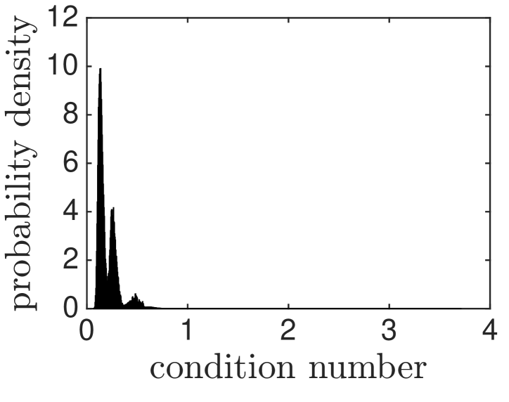
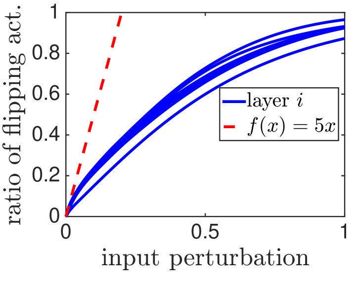
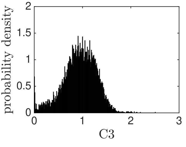
Figure 6.1: Verifying the conditions of Theorem a 10 layer perceptron with 1000 hidden units in each layer, i.e. more than 10,000,000 parameters on MNIST. We have numerically checked that all values are within the displayed range. Left: $C1$: condition number of the network, i.e. $\frac{1}{\mu}$. Middle: $C2$: the ratio of activations that flip based on magnitude of perturbation. Right: $C3:$ the ratio of norm of incoming weights to each hidden units with respect to average of the same quantity over hidden units in the layer.

Additionally the conditions $C1-C3$ actually hold for networks trained in practice as we verify in Figure nd our experiments suggest that, $\mu\geq 1/4,C2\leq 5$ and $C3\leq 3$. More details on the verification and comparing the conditions on learned network with those of random weights, are presented in Section

missing

Proof of Theorem e bound the expectation as follows:

$$\mathbb{E}{\left\lvert{\hat{\ell}(f_{\mathbf{w}+\mathbf{u}}(x))-\hat{\ell}(f_{\mathbf{w}}(x))}\right\rvert}$$

$$\quad\quad\leq C_{L}\mathbb{E}\|f_{\mathbf{w}+\mathbf{u}}(x)-f_{\mathbf{w}}(x)\|_{F}$$

$$\quad\quad\stackrel{{\scriptstyle(i)}}{{=}}C_{L}\mathbb{E}\|(W+\mathbf{u})_{d}\left(\Pi_{i=1}^{d-1}\widehat{D}_{i}(W+\mathbf{u})_{i}\right)*x-W_{d}\left(\Pi_{i=1}^{d-1}D_{i}W_{i}\right)*x\|_{F}$$

$$\quad\quad\leq C_{L}\mathbb{E}\|(W+\mathbf{u})_{d}\left(\Pi_{i=1}^{d-1}D_{i}(W+\mathbf{u})_{i}\right)*x-W_{d}\left(\Pi_{i=1}^{d-1}D_{i}W_{i}\right)*x\|_{F}$$

$$\quad\quad\quad\quad+C_{L}\mathbb{E}\|(W+\mathbf{u})_{d}\left(\Pi_{i=1}^{d-1}\widehat{D}_{i}(W+\mathbf{u})_{i}\right)*x-(W+\mathbf{u})_{d}\left(\Pi_{i=1}^{d-1}D_{i}(W+\mathbf{u})_{i}\right)*x\|_{F}$$

$$\quad\quad\leq C_{L}\mathbb{E}\|(W+\mathbf{u})_{d}\left(\Pi_{i=1}^{d-1}D_{i}(W+\mathbf{u})_{i}\right)*x-W_{d}\left(\Pi_{i=1}^{d-1}D_{i}W_{i}\right)*x\|_{F}+C_{L}\mathbb{E}\|Err_{d}\|_{F},$$ (6.2.1)

where $Err_{d}=\|(W+\mathbf{u})_{d}\left(\Pi_{i=1}^{d-1}\widehat{D}_{i}(W+\mathbf{u})_{i}\right)*x-(W+\mathbf{u})_{d}\left(\Pi_{i=1}^{d-1}D_{i}(W+\mathbf{u})_{i}\right)*x\|_{F}$. $(i)$ $\widehat{D}_{i}$ is the diagonal matrix with 0’s and 1’s corresponding to the activation pattern of the perturbed network $f_{\mathbf{w}+\mathbf{u}}(x)$.

The first term in the equation (6.2.1) corresponds to error due to perturbation of a network with unchanged activations (linear network). Intuitively this is small when any subset of successive layers of the network do no interact weakly with each other (not orthogonal to each other). Condition $C1$ captures this intuition and we bound this error in Lemma lemma Let $U_i$ be a random $h_i ×h_i-1$ matrix with each entry distributed according to $N(0,σ_i^2)$. Then, under the condition $C1$,

$$\mathbb{E}\|(W+\mathbf{u})_d\left(\Pi_{i=1}^{d-1}D_{i}(W+\mathbf{u})_i\right)*x-W_d\left(\Pi_{i=1}^{d-1}D_{i}W_i\right)*x\|_F\\ \leq\left(\Pi_{i=1}^d\left(1+\frac{\sigma_i\sqrt{h_ih_{i-1}}}{\mu^2\|D_iW_i\|_F}\right)-1\right)\|f_\mathbf{w}(x)\|_F.$$

The second term in the equation (6.2.1) captures the perturbation error due to change in activations. If a tiny perturbation can cause exponentially many changes in number of active nodes, then that network will have huge sharpness. Condition $C2$ and $C3$ essentially characterize the behavior of sensitivity of activation patterns to perturbations, leading to a bound on this term in Lemma lemma Let $U_i$ be a random $h_i ×h_i-1$ matrix with each entry distributed according to $N(0,σ_i^2)$. Then, under the conditions $C1$, $C2$ and $C3$, with probability $≥1-δ$, for all $ 1 ≤k ≤d$, $$∥^D_k -D_k∥_1 ≤O ( C_2 h_k C_δ σ_k ∥f^k-1_w∥_F ) $$ and $$E[∥] Err_k∥_F ≤O ( Π_i=1^k ( 1+γ_iC_2 C_3)(Π_i=1^k (1+ γ_i C_δ C_2) - 1)∥f^k_w∥_F ).$$ where $γ_i = σ_i h_ih_i-1μ^2 ∥D_iW_i∥_F$ and $C_δ=2ln(dh/δ)$.

Hence, from Lemma d Lemma get,

$$\mathbb{E}{\left\lvert{\hat{\ell}(f_{\mathbf{w}+\mathbf{u}}(x))-\hat{\ell}(f_{\mathbf{w}}(x))}\right\rvert}$$

$$\leq\left[\Pi_{i=1}^{d}\left(1+\gamma_{i}\right)-1+\Pi_{i=1}^{d}\left(1+\gamma_{i}C_{2}C_{3}\right)\left(\Pi_{i=1}^{d}(1+\gamma_{i}C_{\delta}C_{2})-1\right)\right]C_{L}\|f_{\mathbf{w}}(x)\|_{F}.$$

Here $\gamma_{i}=\frac{\sigma_{i}\sqrt{h_{i}}\sqrt{h_{i-1}}}{\mu^{2}\|D_{i}W_{i}\|_{F}}$. Substituting the above bound on expected sharpness in the PAC-Bayes result (equation (3.4.4)), gives the result.

6.3 Supporting Results

6.3.1 Supporting Lemma

Lemma 25.

Let $A$ ,$B$ be $n_{1}\times n_{2}$ and $n_{3}\times n_{4}$ matrices and $\mathbf{u}$ be a $n_{2}\times n_{3}$ entrywise random Gaussian matrix with $\mathbf{u}_{ij}\sim\mathcal{N}(0,\sigma)$. Then,

$$\mathbb{E}\left[\|A*\mathbf{u}*B\|_{F}\right]\leq\sigma\|A\|_{F}\|B\|_{F}.$$

Proof.

By Jensen’s inequality,

$$\mathbb{E}\left[\|A*\mathbf{u}*B\|_{F}\right]^{2} \leq\mathbb{E}\left[\|A*\mathbf{u}*B\|_{F}^{2}\right]$$

$$=\mathbb{E}\left[\left(\sum_{ij}\sum_{kl}A_{ik}\mathbf{u}_{kl}B_{lj}\right)^{2}\right]$$

$$=\sum_{ij}\sum_{kl}A_{ik}^{2}\mathbb{E}\left[\mathbf{u}_{kl}^{2}\right]B_{lj}^{2}$$

$$=\sigma^{2}\|A\|_{F}^{2}\|B\|_{F}^{2}.$$

∎

6.3.2 Conditions in Theorem  missing

In this section, we compare the conditions in Theorem  a learned network with that of its random initialization. We trained a 10-layer feedforward network with 1000 hidden units in each layer on MNIST dataset. Figures fig:conditions_verify3 and mpare condition $C1$, $C2$ and $C3$ on learned weights to that of random initialization respectively. Interestingly, we observe that the network with learned weights is very similar to its random initialization in terms of these conditions.

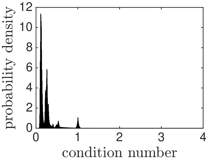
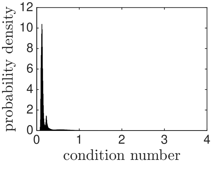
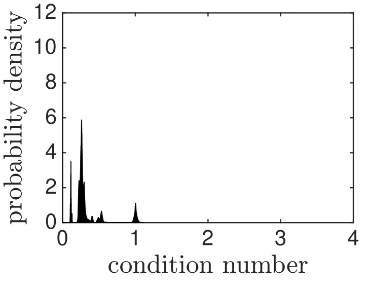
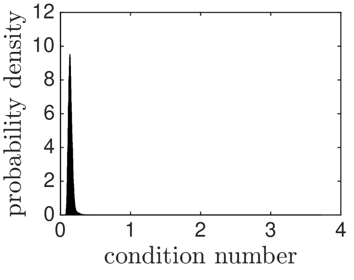
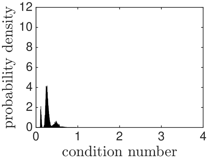
Figure 6.2: Condition $C1$: condition number $\frac{1}{\mu}$ of the network and its decomposition to two cases for random initialization and learned weights. Top: random initialization Bottom: learned weights. Left: distribution of all combinations of $a\leq c\leq b-1$. Middle: when $a<c<b-1$. Right: when $c=a$ or $c=b-1$.

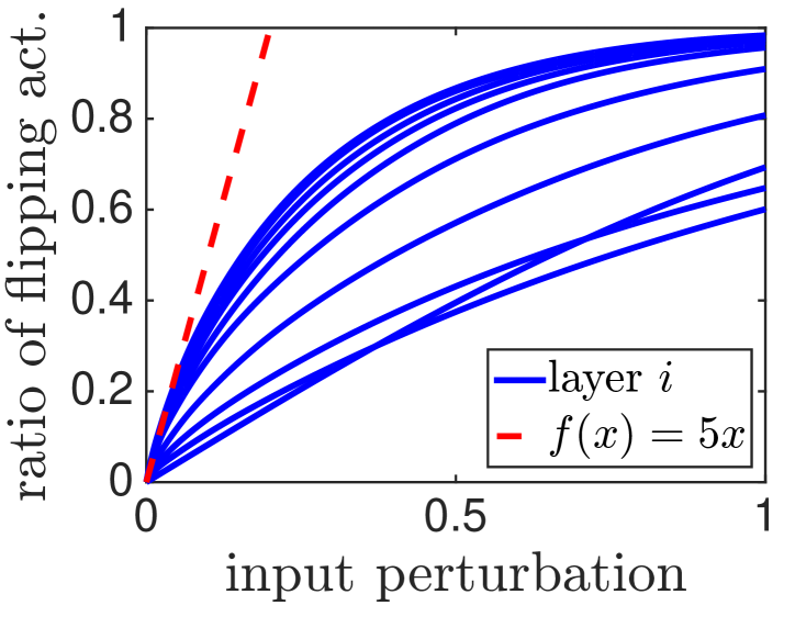
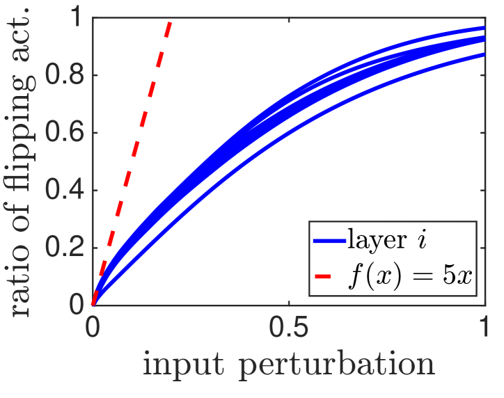
Figure 6.3: Ratio of activations that flip based on the magnitude of perturbation. Left: random initialization. Middle: learned weights. Right: learned weights (zoomed in).

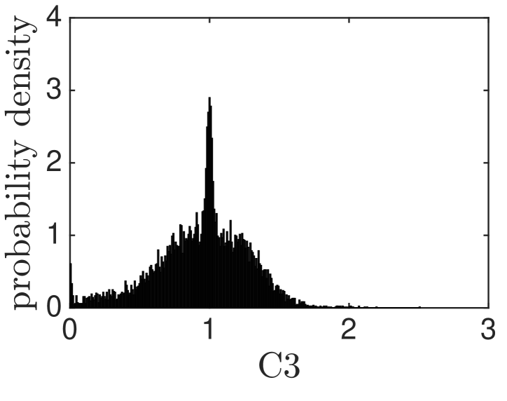
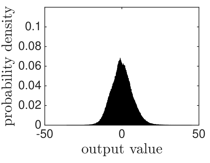
Figure 6.4: From left to right: Condition $C3$ for random initialization and learned network, output values for random and learned network

6.4 Proofs

6.4.1 Proof of Lemma missing

Proof.

Let $\Delta_{i}={\left\lvert{f^{i}_{\mathbf{w}+\mathbf{u}}(\mathbf{x})-f^{i}_{\mathbf{w}}(\mathbf{x})}\right\rvert}_{2}$ be the sharpness of layer $i$. We will prove using induction that for any $i\geq 0$:

$$\Delta_{i}\leq\left(1+\frac{1}{d}\right)^{i}\left(\prod_{j=1}^{i}\left\lVert{W_{j}}\right\rVert_{2}\right){\left\lvert{\mathbf{x}}\right\rvert}_{2}\sum_{j=1}^{i}\frac{\left\lVert{U_{j}}\right\rVert_{2}}{\left\lVert{W_{j}}\right\rVert_{2}}.$$

The above inequality together with $\left(1+\frac{1}{d}\right)^{d}\leq e$ proves the lemma statement. The induction base clearly holds since $\Delta_{0}={\left\lvert{\mathbf{x}-\mathbf{x}}\right\rvert}_{2}=0$. For any $i\geq 1$, we have the following:

$$\Delta_{i+1} ={\left\lvert{\left(W_{i+1}+U_{i+1}\right)\phi_{i}(f^{i}_{\mathbf{w}+\mathbf{u}}(\mathbf{x}))-W_{i+1}\phi_{i}(f^{i}_{\mathbf{w}}(\mathbf{x}))}\right\rvert}_{2}$$

$$={\left\lvert{\left(W_{i+1}+U_{i+1}\right)\left(\phi_{i}(f^{i}_{\mathbf{w}+\mathbf{u}}(\mathbf{x}))-\phi_{i}(f^{i}_{\mathbf{w}}(\mathbf{x}))\right)+U_{i+1}\phi_{i}(f^{i}_{\mathbf{w}}(\mathbf{x}))}\right\rvert}_{2}$$

$$\leq\left(\left\lVert{W_{i+1}}\right\rVert_{2}+\left\lVert{U_{i+1}}\right\rVert_{2}\right){\left\lvert{\phi_{i}(f^{i}_{\mathbf{w}+\mathbf{u}}(\mathbf{x}))-\phi_{i}(f^{i}_{\mathbf{w}}(\mathbf{x}))}\right\rvert}_{2}+\left\lVert{U_{i+1}}\right\rVert_{2}{\left\lvert{\phi_{i}(f^{i}_{\mathbf{w}}(\mathbf{x}))}\right\rvert}_{2}$$

$$\leq\left(\left\lVert{W_{i+1}}\right\rVert_{2}+\left\lVert{U_{i+1}}\right\rVert_{2}\right){\left\lvert{f^{i}_{\mathbf{w}+\mathbf{u}}(\mathbf{x})-f^{i}_{\mathbf{w}}(\mathbf{x})}\right\rvert}_{2}+\left\lVert{U_{i+1}}\right\rVert_{2}{\left\lvert{f^{i}_{\mathbf{w}}(\mathbf{x})}\right\rvert}_{2}$$

$$=\Delta_{i}\left(\left\lVert{W_{i+1}}\right\rVert_{2}+\left\lVert{U_{i+1}}\right\rVert_{2}\right)+\left\lVert{U_{i+1}}\right\rVert_{2}{\left\lvert{f^{i}_{\mathbf{w}}(\mathbf{x})}\right\rvert}_{2},$$

where the last inequality is by the Lipschitz property of the activation function and using $\phi(0)=0$. The $\ell_{2}$ norm of outputs of layer $i$ is bounded by ${\left\lvert{\mathbf{x}}\right\rvert}_{2}\Pi_{j=1}^{i}\left\lVert{W_{j}}\right\rVert_{2}$ and by the lemma assumption we have $\left\lVert{U_{i+1}}\right\rVert_{2}\leq\frac{1}{d}\left\lVert{W_{i+1}}\right\rVert_{2}$. Therefore, using the induction step, we get the following bound:

$$\Delta_{i+1} \leq\Delta_{i}\left(1+\frac{1}{d}\right)\left\lVert{W_{i+1}}\right\rVert_{2}+\left\lVert{U_{i+1}}\right\rVert_{2}{\left\lvert{\mathbf{x}}\right\rvert}_{2}\prod_{j=1}^{i}\left\lVert{W_{j}}\right\rVert_{2}$$

$$\leq\left(1+\frac{1}{d}\right)^{i+1}\left(\prod_{j=1}^{i+1}\left\lVert{W_{j}}\right\rVert_{2}\right){\left\lvert{\mathbf{x}}\right\rvert}_{2}\sum_{j=1}^{i}\frac{\left\lVert{U_{j}}\right\rVert_{2}}{\left\lVert{W_{j}}\right\rVert_{2}}+\frac{\left\lVert{U_{i+1}}\right\rVert_{2}}{\left\lVert{W_{i+1}}\right\rVert_{2}}{\left\lvert{\mathbf{x}}\right\rvert}_{2}\prod_{j=1}^{i+1}\left\lVert{W_{i}}\right\rVert_{2}$$

$$\leq\left(1+\frac{1}{d}\right)^{i+1}\left(\prod_{j=1}^{i+1}\left\lVert{W_{j}}\right\rVert_{2}\right){\left\lvert{\mathbf{x}}\right\rvert}_{2}\sum_{j=1}^{i+1}\frac{\left\lVert{U_{j}}\right\rVert_{2}}{\left\lVert{W_{j}}\right\rVert_{2}}.$$

This completes the proof. ∎

6.4.2 Proof of Lemma missing

Proof.

Define $g_{\{W_{-i-j},\mathbf{u}_{i,j}\}}(x)$ as the network $f_{W}$ with weights in layers $i,j,$, $W_{i},W_{j}$ replaced by $U_{i},\mathbf{u}_{j}$. Hence,

$$\|(W+\mathbf{u})_{d} \left(\Pi_{i=1}^{d-1}D_{i}(W+\mathbf{u})_{i}\right)*x-W_{d}\left(\Pi_{i=1}^{d-1}D_{i}W_{i}\right)*x\|_{F}$$

$$\leq\|\sum_{i}g(\{W_{-i},U_{i}\},x)\|_{F}+\|\sum_{i,j}g(\{W_{-i-j},\mathbf{u}_{i,j}\},x)\|_{F}+\cdots+\|f_{\mathbf{u}}(x)\|_{F}$$ (6.4.1)

Base case: First we show the bound for terms with one noisy layer. Let $g(\{W_{-k},\mathbf{u}_{k}\},x)$ denote $f_{W}(x)$ with weights in layer $k$, $W_{k}$ replaced by $\mathbf{u}_{k}$. Now notice that,

$$\mathbb{E}\|g(\{W_{-k},\mathbf{u}_{k}\},x)\|_{F} =\mathbb{E}\|W_{d}\Pi_{i=k+1}^{d-1}D_{i}W_{i}*D_{k}\mathbf{u}_{k}*\left(\Pi_{i=1}^{k-1}D_{i}W_{i}\right)*x\|_{F}$$

$$\stackrel{{\scriptstyle(i)}}{{\leq}}\sigma_{k}\|W_{d}\Pi_{i=k+1}^{d-1}D_{i}W_{i}\|_{F}\|\|\left(\Pi_{i=1}^{k-1}D_{i}W_{i}\right)*x\|_{F}$$

$$\stackrel{{\scriptstyle(ii)}}{{\leq}}\sigma_{k}\frac{\sqrt{h_{k}h_{k-1}}}{\mu^{2}\|D_{k}W_{k}\|_{F}}\|W_{d}\left(\Pi_{i=1}^{d-1}D_{i}W_{i}\right)*x\|_{F}$$

$$=\sigma_{k}\frac{\sqrt{h_{k}h_{k-1}}}{\mu^{2}\|D_{k}W_{k}\|_{F}}\|f_{W}(x)\|_{F}.$$

$(i)$ follows from Lemma (ii)$followsfromcondition$C1$.\par\noindent{\bf Inductionstep:}Letforanyset$s ⊂[d], |s| =k$,thefollowingholds:$$\mathbb{E}\|g(\{W_{-i},\mathbf{u}_{i}\}_{i\in s},x)\|_{F}\leq\|f_{W}(x)\|_{F}\Pi_{i\in s}\sigma_{i}\frac{\sqrt{h_{i}h_{i-1}}}{\mu^{2}\|D_{i}W_{i}\|_{F}}.$$\par Wewillprovethisnowfortermswith$k+1$noisylayers.\begin{aligned} \mathbb{E}\|g(\{W_{-i},\mathbf{u}_{i}\}_{i\in s\cup\{j\}},x)\|_{F}&\leq\sigma_{j}\frac{\sqrt{h_{j}h_{j-1}}}{\mu^{2}\|D_{j}W_{j}\|}\mathbb{E}\|g(\{W_{-i},\mathbf{u}_{i}\}_{i\in s},x)\|_{F}\\ &\leq\sigma_{j}\frac{\sqrt{h_{j}h_{j-1}}}{\mu^{2}\|D_{j}W_{j}\|}\|f_{W}(x)\|_{F}\Pi_{i\in s}\sigma_{i}\frac{\sqrt{h_{i}h_{i-1}}}{\mu^{2}\|D_{i}W_{i}\|_{F}}\\ &=\|f_{W}(x)\|_{F}\Pi_{i\in s\cup\{j\}}\sigma_{i}\frac{\sqrt{h_{i}h_{i-1}}}{\mu^{2}\|D_{i}W_{i}\|_{F}}\end{aligned}\par Substitutingtheaboveexpressioninequation~{}\eqref{eq:lem_linear1}gives,\begin{multline*}\|(W+\mathbf{u})_{d}\left(\Pi_{i=1}^{d-1}D_{i}(W+\mathbf{u})_{i}\right)*x-W_{d}\left(\Pi_{i=1}^{d-1}D_{i}W_{i}\right)*x\|_{F}\\ \leq\left(\Pi_{i=1}^{d}\left(1+\frac{\sigma_{i}\sqrt{h_{i}}\sqrt{h_{i-1}}}{\mu^{2}\|D_{i}W_{i}\|_{F}}\right)-1\right)\|f_{W}(x)\|_{F}.\end{multline*}\|(W+\mathbf{u})_{d}\left(\Pi_{i=1}^{d-1}D_{i}(W+\mathbf{u})_{i}\right)*x-W_{d}\left(\Pi_{i=1}^{d-1}D_{i}W_{i}\right)*x\|_{F}\\ \leq\left(\Pi_{i=1}^{d}\left(1+\frac{\sigma_{i}\sqrt{h_{i}}\sqrt{h_{i-1}}}{\mu^{2}\|D_{i}W_{i}\|_{F}}\right)-1\right)\|f_{W}(x)\|_{F}.\par\qed\end@proof\par$

6.4.3 Proof of Lemma missing

Proof.

We prove this lemma by induction on $k$. Recall that $\widehat{D}_{i}$ is the diagonal matrix with 0’s and 1’s corresponding to the activation pattern of the perturbed network $f_{W+\mathbf{u}}(x)$. Let $1_{E}$ denote the indicator function, that is $1$ if the event $E$ is true, $0$ else. We also use $f_{W}^{k}(x)$ to denote the network truncated to level $k$, in particular $f_{W}^{k}(x)=\Pi_{i=1}^{k}D_{k}W_{k}x$.

Base case:

$$\|\widehat{D}_{1}-D_{1}\|_{1}=\sum_{i}1_{\left\langle(W+\mathbf{u})_{1,i},x\right\rangle*\left\langle W_{1,i},x\right\rangle<0}=\sum_{i}1_{\left\langle(W)_{1,i},x\right\rangle^{2}<-\left\langle(\mathbf{u})_{1,i},x\right\rangle*\left\langle(W)_{1,i},x\right\rangle}\\ \leq\sum_{i}1_{{\left\lvert{\left\langle(W)_{1,i},x\right\rangle}\right\rvert}<{\left\lvert{\left\langle(\mathbf{u})_{1,i},x\right\rangle}\right\rvert}}.$$

Since $\mathbf{u}_{1}$ is a random Gaussian matrix, and $\|x\|\leq 1$, for any $i$, ${\left\lvert{\left\langle(\mathbf{u})_{1,i},x\right\rangle}\right\rvert}\leq\sigma_{1}(1+\delta_{1})\sqrt{2\ln(h_{1})}$ with probability greater than $1-\delta_{1}$. Hence, with probability $\geq 1-\delta_{1}$,

$$\|\widehat{D}_{1}-D_{1}\|_{1}\leq\sum_{i}1_{{\left\lvert{\left\langle(W)_{1,i},x\right\rangle}\right\rvert}\leq\sigma_{1}\sqrt{20\ln(h_{1})}}\leq C_{2}h_{1}\sigma_{1}(1+\delta_{1})\sqrt{2\ln(h_{1})}=C_{2}h_{1}\sigma_{1}C_{\delta_{1}}.$$

This completes the base case for $k=1$. $\widehat{D}_{1}$ is a random variable that depends on $\mathbf{u}_{1}$. Hence, in the remainder of the proof, to avoid this dependence, we separately bound $\widehat{D}_{1}-D$ using the expression above and compute expectation only with respect to $\mathbf{u}_{1}$. With probability $\geq 1-\delta_{1}$,

$$\mathbb{E}\|Err_{1}\|_{F} =\mathbb{E}\|\widehat{D}_{1}*(W+\mathbf{u})_{1}x-D_{1}*(W+\mathbf{u})_{1}x\|_{F}$$

$$\leq\mathbb{E}\|(\widehat{D}_{1}-D_{1})*W_{1}x\|_{F}+\mathbb{E}\|(\widehat{D}_{1}-D_{1})*\mathbf{u}_{1}x\|_{F}$$

$$\stackrel{{\scriptstyle(i)}}{{\leq}}\sqrt{C_{2}h_{1}\sigma_{1}C_{\delta_{1}}}\sigma_{1}+\sqrt{C_{2}h_{1}\sigma_{1}C_{\delta_{1}}}\sigma_{1}$$

$$=2\sqrt{C_{2}h_{1}\sigma_{1}C_{\delta_{1}}}\sigma_{1}.$$

$(i)$ follows because, each hidden node in $\mathbb{E}\|(\widehat{D}_{1}-D_{1})*W_{1}x\|_{F}$ has norm less than $\sigma_{1}C_{\delta_{1}}$ (as it changed its activation), number of such units is less than $C_{2}h_{1}\sigma_{1}C_{\delta_{1}}$.

$k=1$ case does not capture all the intricacies and dependencies of higher layer networks. Hence we also evaluate the bounds for $k=2$.

$$\|\widehat{D}_{2}-D_{2}\|_{1}\leq\sum_{i}1_{\left\langle(W+\mathbf{u})_{2,i},f^{1}_{W+\mathbf{u}}\right\rangle*\left\langle W_{2,i},f^{1}_{W}\right\rangle\leq 0}\leq\sum_{i}1_{{\left\lvert{\left\langle W_{2,i},f^{1}_{W}\right\rangle}\right\rvert}\leq{\left\lvert{\left\langle\mathbf{u}_{2,i},f^{1}_{W+\mathbf{u}}\right\rangle}\right\rvert}+{\left\lvert{\left\langle W_{2,i},f^{1}_{W+\mathbf{u}}-f^{1}_{W}\right\rangle}\right\rvert}}$$

Let $C_{\delta_{2}}=(1+\delta_{2})\sqrt{2\ln(h_{2})}$. Then, with probability $\geq 1-\delta_{1}-\delta_{2}$,

$${\left\lvert{\left\langle\mathbf{u}_{2,i},f^{1}_{W+\mathbf{u}}\right\rangle}\right\rvert}+{\left\lvert{\left\langle W_{2,i},f^{1}_{W+\mathbf{u}}-f^{1}_{W}\right\rangle}\right\rvert}$$

$$\leq C_{\delta_{2}}\sigma_{2}\left(\|f^{1}_{W}\|_{F}+2\sqrt{C_{2}h_{1}\sigma_{1}C_{\delta_{1}}}\sigma_{1}\right)+\|W_{2,i}\|2\sqrt{C_{2}h_{1}\sigma_{1}C_{\delta_{1}}}\sigma_{1}$$

$$\leq C_{\delta_{2}}\sigma_{2}\left(\|f^{1}_{W}\|_{F}+2\sqrt{C_{2}h_{1}\sigma_{1}C_{\delta_{1}}}\sigma_{1}\right)+C_{3}\frac{\|D_{2}W_{2}\|_{F}}{\sqrt{h_{2}}}2\sqrt{C_{2}h_{1}\sigma_{1}C_{\delta_{1}}}\sigma_{1}$$

$$\stackrel{{\scriptstyle(i)}}{{\leq}}C_{\delta_{2}}\sigma_{2}\left(\|f^{1}_{W}\|_{F}+2\sqrt{\frac{\hat{\sigma_{1}}}{\sqrt{h_{i}+h_{i-1}}}}\hat{\sigma_{1}}\right)+2\hat{\sigma_{1}}\frac{C_{3}\|f_{W}(x)\|_{F}^{\nicefrac{{1}}{{d}}}}{\mu}\sqrt{\frac{\hat{\sigma_{1}}}{\sqrt{h_{i}+h_{i-1}}}}$$

$$=C_{\delta_{2}}\sigma_{2}\left(\|f^{1}_{W}\|_{F}+\gamma_{1}\hat{\sigma_{1}}\right)+\frac{C_{3}\|f_{W}(x)\|_{F}^{\nicefrac{{1}}{{d}}}}{\mu}\gamma_{1}\hat{\sigma_{1}}$$

where, $\gamma_{i}=2\sqrt{\frac{\hat{\sigma_{1}}}{\sqrt{h_{i}+h_{i-1}}}}$. $(i)$ follows from condition $C1$, which results in $\Pi_{i=2}^{d}\frac{\mu\|D_{i}W_{i}\|_{F}}{\sqrt{h_{i}}}\frac{\mu\|D_{1}W_{1}x\|_{F}}{\sqrt{h_{1}}}\leq\|f_{W}(x)\|_{F}$. Hence, if we consider the rebalanced network where all layers have same values for $\frac{\mu\|D_{i}W_{i}\|_{F}}{\sqrt{h_{i}}}$, we get, $\frac{\mu\|D_{i}W_{i}\|_{F}}{\sqrt{h_{i}}}\leq\|f_{W}(x)\|_{F}^{\nicefrac{{1}}{{d}}}$. Also the above equations follow from setting, $\sigma_{i}=\frac{\hat{\sigma}_{i}}{C_{2}C_{\delta_{i}}\sqrt{h_{i}+h_{i-1}}}$.

Hence, with probability $\geq 1-\delta_{1}-\delta_{2}$,

$$\|\widehat{D}_{2}-D_{2}\|_{1} \leq C_{2}*h_{2}\left(C_{\delta_{2}}\sigma_{2}\left(\|f^{1}_{W}\|_{F}+\gamma_{1}\hat{\sigma_{1}}\right)+\frac{C_{3}\|f_{W}(x)\|_{F}^{\nicefrac{{1}}{{d}}}}{\mu}\gamma_{1}\hat{\sigma_{1}}\right).$$

Since, we choose $\sigma_{i}$ to scale as some small number $O(\sigma)$, in the above expression the first term scales as $O(\sigma)$ and the last two terms decay at least as $O(\sigma^{3}{2})$. Hence we do not include them in the computation of $Err$.

$$\mathbb{E}\|Err_{2}\|_{F} =\mathbb{E}\|\widehat{D}_{2}(W+\mathbf{u})_{2}*\widehat{D}_{1}*(W+\mathbf{u})_{1}x-D_{2}(W+\mathbf{u})_{2}*D_{1}*(W+\mathbf{u})_{1}x\|_{F}$$

$$\leq\mathbb{E}\|(\widehat{D}_{2}-D_{2})(W+\mathbf{u})_{2}*(\widehat{D}_{1}-D_{1})*(W+\mathbf{u})_{1}x\|_{F}+\mathbb{E}\|D_{2}(W+\mathbf{u})_{2}*(\widehat{D}_{1}-D_{1})*(W+\mathbf{u})_{1}x\|_{F}$$

$$\quad\quad+\mathbb{E}\|(\widehat{D}_{2}-D_{2})(W+\mathbf{u})_{2}*D_{1}*(W+\mathbf{u})_{1}x\|_{F}.$$

We will bound now the first term in the above expression. With probability $\geq 1-\delta_{1}-\delta_{2}$,

$$\mathbb{E} \|(\widehat{D}_{2}-D_{2})(W+\mathbf{u})_{2}*(\widehat{D}_{1}-D_{1})*(W+\mathbf{u})_{1}x\|_{F}$$

$$\leq\mathbb{E}\|(\widehat{D}_{2}-D_{2})W_{2}*(\widehat{D}_{1}-D_{1})*W_{1}x\|_{F}+\mathbb{E}\|(\widehat{D}_{2}-D_{2})W_{2}*(\widehat{D}_{1}-D_{1})*\mathbf{u}_{1}x\|_{F}$$

$$\quad\quad+\mathbb{E}\|(\widehat{D}_{2}-D_{2})\mathbf{u}_{2}*(\widehat{D}_{1}-D_{1})*W_{1}x\|_{F}+\mathbb{E}\|(\widehat{D}_{2}-D_{2})\mathbf{u}_{2}*(\widehat{D}_{1}-D_{1})*\mathbf{u}_{1}x\|_{F}$$

$$\leq 2\sqrt{C_{2}*h_{2}C_{\delta_{2}}\sigma_{2}\|f^{1}_{W}\|_{F}}C_{\delta_{2}}\sigma_{2}\|f^{1}_{W}\|_{F}\sqrt{C_{2}*h_{1}*C_{\delta_{1}}\sigma_{1}}C_{\delta_{1}}\sigma_{1}$$

$$\quad\quad+2\sqrt{C_{2}*h_{2}C_{\delta_{2}}\sigma_{2}\|f^{1}_{W}\|_{F}}C_{\delta_{2}}\sigma_{2}\sqrt{h_{1}}\sqrt{C_{2}*h_{1}*C_{\delta_{1}}\sigma_{1}}C_{\delta_{1}}\sigma_{1}+O(\sigma^{2})$$

$$\leq 4\|f_{W}^{2}\|_{F}\frac{C_{\delta_{2}}\sigma_{2}C_{\delta_{1}}\sigma_{1}\sqrt{h_{1}}}{\mu\|D_{2}W_{2}\|_{F}}\Pi_{i=1}^{2}\sqrt{C_{2}h_{i}C_{\delta_{i}}\sigma_{i}}.$$

Induction step:

Now we assume the statement for all $i\leq k$ and prove it for $k+1$. $\|\widehat{D}_{k}-D_{k}\|_{1}\leq C_{2}h_{k}C_{\delta_{k}}\sigma_{k}\|f^{k-1}_{W}\|_{F}$ and ${\mathbb{E}\left[{\|}\right]}Err_{k}\|_{F}\leq\Pi_{i=1}^{k}\left(1+\frac{\sigma_{i}\sqrt{h_{i-1}}}{\mu^{2}C^{i}_{2,\infty}C_{2}}\right)\left(\Pi_{i=1}^{k}(1+\frac{\hat{\sigma_{i}}^{3/2}}{C_{2}})-1\right)\|f^{k}_{w}\|_{F}$. Now we prove the statement for $k+1$.

$$\|\widehat{D}_{k+1}-D_{k+1}\|_{1} =\sum_{i}1_{\left\langle(W+\mathbf{u})_{k+1,i},\Pi_{i=1}^{k}\widehat{D}_{i}(W+\mathbf{u})_{i}*x\right\rangle*\left\langle W_{2,i},D_{1}W_{1}x\right\rangle\leq 0}$$

$$\leq\sum_{i}1_{{\left\lvert{\left\langle W_{k+1,i},\Pi_{i=1}^{k}\widehat{D}_{i}(W+\mathbf{u})_{i}*x\right\rangle}\right\rvert}\leq{\left\lvert{\left\langle\mathbf{u}_{k+1,i},\Pi_{i=1}^{k}\widehat{D}_{i}(W+\mathbf{u})_{i}*x\right\rangle}\right\rvert}}$$

$$=\sum_{i}1_{{\left\lvert{\left\langle W_{k+1,i},f^{k}_{W+\mathbf{u}}\right\rangle}\right\rvert}\leq{\left\lvert{\left\langle\mathbf{u}_{k+1,i},f^{k}_{W+\mathbf{u}}\right\rangle}\right\rvert}}$$

$$\leq\sum_{i}1_{{\left\lvert{\left\langle W_{k+1,i},f^{k}_{W}\right\rangle}\right\rvert}\leq{\left\lvert{\left\langle\mathbf{u}_{k+1,i},f^{k}_{W}\right\rangle}\right\rvert}+{\left\lvert{\left\langle\mathbf{u}_{k+1,i},f^{k}_{W+\mathbf{u}}-f^{k}_{W}\right\rangle}\right\rvert}+{\left\lvert{\left\langle W_{k+1,i},f^{k}_{W+\mathbf{u}}-f^{k}_{W}\right\rangle}\right\rvert}}$$

Hence, with probability $\geq 1-\sum_{i=1}^{k}\delta_{i}$,

$$\|\widehat{D}_{k+1}-D_{k+1}\|_{1} \leq C_{2}h_{k+1}\left[C_{\delta_{k}}\sigma_{k+1}(\|f^{k}_{W}\|_{F}+\|f^{k}_{W+\mathbf{u}}-f^{k}_{W}\|_{F})+\|W_{k+1,i}\|\|f^{k}_{W+\mathbf{u}}-f^{k}_{W}\|_{F}\right]$$

$$\leq C_{2}h_{k+1}C_{\delta_{k}}\sigma_{k+1}\|f^{k}_{W}\|_{F}+C_{2}h_{k+1}C_{\delta_{k}}\sigma_{k+1}\|f^{k}_{W+\mathbf{u}}-f^{k}_{W}\|_{F}+C_{2}h_{k+1}\|W_{k+1,i}\|\|f^{k}_{W+\mathbf{u}}-f^{k}_{W}\|_{F}.$$

Now we will show that the last two terms in the above expression scale as $O(\sigma^{2})$. For that, first notice that $\|f^{k}_{W+\mathbf{u}}-f^{k}_{W}\|_{F}\leq\left(\Pi_{i=1}^{k}\left(1+\frac{\sigma_{i}\sqrt{h_{i}h_{i-1}}}{\mu^{2}\|D_{i}W_{i}\|_{F}}\right)-1\right)\|f_{W}(x)\|_{F}+Err_{k}$, from lemma ote that the second term in the above expression clearly scale as $O(\sigma^{2})$.

Hence,

$$\|\widehat{D}_{k+1}-D_{k+1}\|_{1}\leq C_{2}h_{k+1}C_{\delta_{k}}\sigma_{k+1}\|f^{k}_{W}\|_{F}+O(\sigma^{2})$$

$$\|Err_{k+1}\| =\|f^{k+1}_{W+\mathbf{u}}-\tilde{f}^{k+1}_{W+\mathbf{u}}\|_{F}$$

$$=\|\widehat{D}_{k+1}(W+\mathbf{u})_{k+1}\Pi_{i=1}^{k+1}\widehat{D}_{i}(W+\mathbf{u})_{i}x-D_{k+1}(W+\mathbf{u})_{k+1}\Pi_{i=1}^{k+1}D_{i}(W+\mathbf{u})_{i}x\|_{F}$$

$$\leq\|(\widehat{D}_{k+1}-D_{k+1})(W+\mathbf{u})_{k+1}\Pi_{i=1}^{k+1}D_{i}(W+\mathbf{u})_{i}x\|_{F}+\|\widehat{D}_{k+1}(W+\mathbf{u})_{k+1}Err_{k}\|_{F}$$

$$\leq\|(\widehat{D}_{k+1}-D_{k+1})(W+\mathbf{u})_{k+1}\Pi_{i=1}^{k+1}D_{i}(W+\mathbf{u})_{i}x\|_{F}+\|(\widehat{D}_{k+1}-D_{k+1})(W+\mathbf{u})_{k+1}Err_{k}\|_{F}$$

$$\quad\quad+\|D_{k+1}(W+\mathbf{u})_{k+1}Err_{k}\|_{F}$$

Substituting the bounds for $\widehat{D}_{k+1}-D_{k+1}$ and $Err_{k}$ gives us, with probability $\geq 1-\sum_{i=1}^{k+1}\delta_{i}$.

$$\mathbb{E}\|Err_{k+1}\| \leq\sqrt{C_{2}h_{k+1}C_{\delta_{k}}\sigma_{k+1}\|f^{k}_{W}\|_{F}}C_{\delta_{k}}\sigma_{k+1}\|f^{k}_{W}\|_{F}\mathbb{E}\|\Pi_{i=1}^{k+1}D_{i}(W+\mathbf{u})_{i}x\|_{F}$$

$$\quad\quad+\mathbb{E}\|Err_{k}\|_{F}\left(\sqrt{C_{2}h_{k+1}C_{\delta_{k}}\sigma_{k+1}\|f^{k}_{W}\|_{F}}C_{\delta_{k}}\sigma_{k+1}\|f^{k}_{W}\|_{F}+\|D_{k+1}W_{k+1}\|_{F}+\sigma_{k+1}\sqrt{h_{k+1}}\right)$$

Now we bound the above terms following the same approach as in proof of Lemma y considering all possible replacements of $W_{i}$ with $U_{i}$. That gives us the result.

∎

Chapter 7 Empirical Investigation

In this chapter we investigate the ability of the discussed measures to explain the different generalization phenomenon.

7.1 Complexity Measures

Capacity control in terms of norm, when using a zero/one loss (i.e. counting errors) requires us in addition to account for scaling of the output of the neural networks, as the loss is insensitive to this scaling but the norm only makes sense in the context of such scaling. For example, dividing all the weights by the same number will scale down the output of the network but does not change the $0/1$ loss, and hence it is possible to get a network with arbitrary small norm and the same $0/1$ loss. Using a scale sensitive losses, such as the cross entropy loss, does address this issue (if the outputs are scaled down toward zero, the loss becomes trivially bad), and one can obtain generalization guarantees in terms of norm and the cross entropy loss.

However, we should be careful when comparing the norms of different models learned by minimizing the cross entropy loss, in particular when the training error goes to zero. When the training error goes to zero, in order to push the cross entropy loss (or any other positive loss that diminish at infinity) to zero, the outputs of the network must go to infinity, and thus the norm of the weights (under any norm) should also go to infinity. This means that minimizing the cross entropy loss will drive the norm toward infinity. In practice, the search is terminated at some finite time, resulting in large, but finite norm. But the value of this norm is mostly an indication of how far the optimization is allowed to progress—using a stricter stopping criteria (or higher allowed number of iterations) would yield higher norm. In particular, comparing the norms of models found using different optimization approaches is meaningless, as they would all go toward infinity.

Instead, to meaningfully compare norms of the network, we should explicitly take into account the scaling of the outputs of the network. One way this can be done, when the training error is indeed zero, is to consider the “margin” of the predictions in addition to the norms of the parameters. We refer to the margin for a single data point $x$ as the difference between the score of the correct label and the maximum score of other labels, i.e.

$$f_{\mathbf{w}}(\mathbf{x})[y_{\text{true}}]-\max_{y\neq y_{\text{true}}}f_{\mathbf{w}}(\mathbf{x})[y]$$ (7.1.1)

In order to measure scale over an entire training set, one simple approach is to consider the “hard margin”, which is the minimum margin among all training points. However, this definition is very sensitive to extreme points as well as to the size of the training set. We consider instead a more robust notion that allows a small portion of data points to violate the margin. For a given training set and small value $\epsilon>0$, we define the margin $\gamma_{\text{margin}}$ as the lowest value of $\gamma$ such that $\lceil\epsilon m\rceil$ data point have margin lower than $\gamma$ where $m$ is the size of the training set. We found empirically that the qualitative and relative nature of our empirical results is almost unaffected by reasonable choices of $\epsilon$ (e.g. between $0.001$ and $0.1$).

The norm-based measures we investigate in this work and their corresponding capacity bounds are as follows :

• $\ell_{2}$ norm with capacity proportional to $\frac{1}{\gamma_{\text{margin}}^{2}}\prod_{i=1}^{d}4\left\lVert{W_{i}}\right\rVert^{2}_{F}$ [NeyTomSre15].

• $\ell_{1}$-path norm with capacity proportional to $\frac{1}{\gamma_{\text{margin}}^{2}}\left(\sum_{j\in\prod_{k=0}^{d}[h_{k}]}{\left\lvert{\prod_{i=1}^{d}2W_{i}[j_{i},j_{i-1}]}\right\rvert}\right)^{2}$[bartlett2002rademacher, NeyTomSre15].

• $\ell_{2}$-path norm with capacity proportional to $\frac{1}{\gamma_{\text{margin}}^{2}}\sum_{j\in\prod_{k=0}^{d}[h_{k}]}\prod_{i=1}^{d}4h_{i}W_{i}^{2}[j_{i},j_{i-1}]$.

• spectral norm with capacity proportional to $\frac{1}{\gamma_{\text{margin}}^{2}}\prod_{i=1}^{d}h_{i}\left\lVert{W_{i}}\right\rVert^{2}_{2}$.

where $\prod_{k=0}^{d}[h_{k}]$ is the Cartesian product over sets $[h_{k}]$. The above bounds indicate that capacity can be bounded in terms of either $\ell_{2}$-norm or $\ell_{1}$-path norm independent of number of parameters. The $\ell_{2}$-path norm dependence on the number of hidden units in each layer is unavoidable. However, it is not clear that the dependence on the number of parameters is needed for the bound based on the spectral norm.

PAC-Bayes Bound

A simple way to instantiate the PAC-Based bound discussed in Section to set $P$ to be a zero mean, $\sigma^{2}$ variance Gaussian distribution. Choosing the perturbation $\epsilon$ to also be a zero mean spherical Gaussian with variance $\sigma^{2}$ in every direction, yields the following guarantee (w.p. $1-\delta$ over the training set):

$${\mathbb{E}_{\epsilon\sim\mathcal{N}(0,\sigma)^{n}}\left[{L(f_{\mathbf{w}+\epsilon})}\right]}\leq\hat{L}(f_{\mathbf{w}})+\underbrace{{\mathbb{E}_{\epsilon\sim\mathcal{N}(0,\sigma)^{n}}\left[{\hat{L}(f_{\mathbf{w}+\epsilon})}\right]}-\hat{L}(f_{\mathbf{w}})}_{\text{expected sharpness}}+4\sqrt{\frac{1}{m}\bigg{(}\underbrace{\frac{\|\mathbf{w}\|_{2}^{2}}{2\sigma^{2}}}_{\text{KL}}+\ln\frac{2m}{\delta}\bigg{)}},$$ (7.1.2)

Another interesting approach is to set the variance of the perturbation to each parameter with respect to the magnitude of the parameter. For example if $\sigma_{i}=\alpha{\left\lvert{w_{i}}\right\rvert}+\beta$, then the KL term in the above expression changes to $\sum_{i}\frac{w_{i}^{2}}{2\sigma_{i}^{2}}$.

The above generalization guarantees give a clear way to think about capacity control jointly in terms of both the expected sharpness and the norm, and as we discussed earlier indicates that sharpness by itself cannot control the capacity without considering the scaling. In the above generalization bound, norms and sharpness interact in a direct way depending on $\sigma$, as increasing the norm by decreasing $\sigma$ causes decrease in sharpness and vice versa. It is therefore important to find the right balance between the norm and sharpness by choosing $\sigma$ appropriately in order to get a reasonable bound on the capacity.

7.2 Experiments Settings

In experiment with different network sizes, we train a two layer perceptron with ReLU activation and varying number of hidden units without Batch Normalization or dropout. In the rest of the experiments, we train a modified version of the VGG architecture [simonyan2014very] with the configuration $2\times[64,3,3,1]$, $2\times[128,3,3,1]$, $2\times[256,3,3,1]$, $2\times[512,3,3,1]$ where we add Batch Normalization before ReLU activations and apply $2\times 2$ max-pooling with window size 2 and dropout after each stack. Convolutional layers are followed by $4\times 4$ average pooling, a fully connected layer with 512 hidden units and finally a linear layer is added for prediction.

In all experiments we train the networks using stochastic gradient descent (SGD) with mini-batch size 64, fixed learning rate 0.01 and momentum 0.9 without weight decay. In all experiments where achieving zero training error is possible, we continue training until the cross-entropy loss is less than $10^{-4}$.

When calculating norms on a network with a Batch Normalization layer, we reparametrize the network to one that represents the exact same function without Batch Normalization as suggested in [neyshabur16]. In all our figures we plot norm divided by margin to avoid scaling issues (see Section where we set the margin over training set $S$ to be $5^{th}$-percentile of the margins of the data points in $S$, i.e. $\text{Prc}_{5}\left\{f_{\mathbf{w}}(x_{i})[y_{i}]-\max_{y\neq y_{i}}f_{\mathbf{w}}(x)[y]|(x_{i},y_{i})\in S\right\}.$ We have also investigated other versions of the margin and observed similar behavior to this notion.

We calculate the sharpness, as suggested in [keskar2016large] - for each parameter $w_{i}$ we bound the magnitude of perturbation by $\alpha({\left\lvert{w_{i}}\right\rvert}+1)$ for $\alpha=5.10^{-4}$. In order to compute the maximum perturbation (maximize the loss), we perform 2000 updates of stochastic gradient ascent starting from the minimum, with mini-batch size 64, fixed step size 0.01 and momentum 0.9.

To compute the expected sharpness, we perturb each parameter $w_{i}$ of the model with noise generated from Gaussian distribution with zero mean and standard deviation, $\alpha(10{\left\lvert{w_{i}}\right\rvert}+1)$. The expected sharpness is average over 1000 random perturbations each of which are averaged over a mini-batch of size 64. We compute the expected sharpness for different choices of $\alpha$. For each value of $\alpha$ the KL divergence can be calculated as $\frac{1}{\alpha^{2}}\sum_{i}\left(\frac{w_{i}}{(10{\left\lvert{w_{i}}\right\rvert}+1)}\right)^{2}$.

7.3 True Labels Vs. Random Labels

As an initial empirical investigation of the appropriateness of the different complexity measures, we compared the complexity (under each of the above measures) of models trained on true versus random labels. We would expect to see two phenomena: first, the complexity of models trained on true labels should be substantially lower than those trained on random labels, corresponding to their better generalization ability. Second, when training on random labels, we expect capacity to increase almost linearly with the number of training examples, since every extra example requires new capacity in order to fit it’s random label. However, when training on true labels we expect the model to capture the true functional dependence between input and output and thus fitting more training examples should only require small increases in the capacity of the network. The results are reported in Figure e indeed observe a gap between the complexity of models learned on real and random labels for all four norms, with the difference in increase in capacity between true and random labels being most pronounced for the $\ell_{2}$ norm and $\ell_{2}$-path norm.

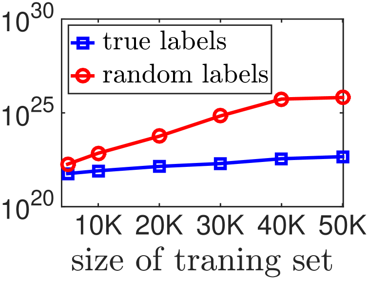
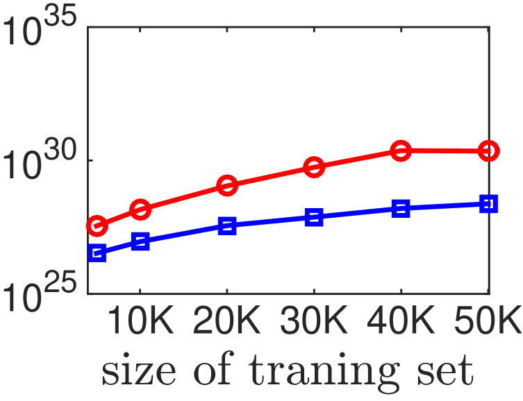
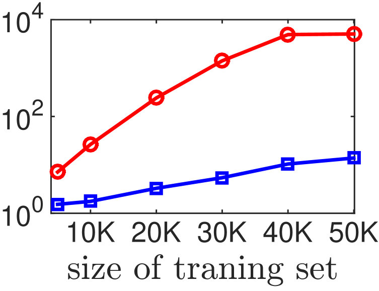
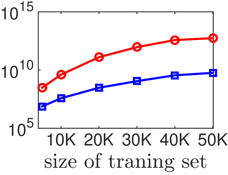
Figure 7.1: Comparing different complexity measures on a VGG network trained on subsets of CIFAR10 dataset with true (blue line) or random (red line) labels. We plot norm divided by margin to avoid scaling issues (see Section where for each complexity measure, we drop the terms that only depend on depth or number of hidden units; e.g. for $\ell_{2}$-path norm we plot $\gamma_{\text{margin}}^{-2}\sum_{j\in\prod_{k=0}^{d}[h_{k}]}\prod_{i=1}^{d}W_{i}^{2}[j_{i},j_{i-1}]$.We also set the margin over training set $S$ to be $5^{th}$-percentile of the margins of the data points in $S$, i.e. $\text{Prc}_{5}\left\{f_{\mathbf{w}}(x_{i})[y_{i}]-\max_{y\neq y_{i}}f_{\mathbf{w}}(\mathbf{x})[y]|(x_{i},y_{i})\in S\right\}$. In all experiments, the training error of the learned network is zero. The plots indicate that these measures can explain the generalization as the complexity of model learned with random labels is always higher than the one learned with true labels. Furthermore, the gap between the complexity of models learned with true and random labels increases as we increase the size of the training set.

In our experiments on PAC-Bayes bound, we observe that looking at both sharpness and norm in Equation intly indeed makes a better predictor for the generalization error. As discussed earlier, dziugaite2017computing numerically optimize the overall PAC-Bayes generalization bound over a family of multivariate Gaussian distributions (different choices of perturbations and priors). Since the precise way the sharpness and KL-divergence are combined is not tight, certainly not in (7.1.2), nor in the more refined bound used by dziugaite2017computing, we prefer shying away from numerically optimizing the balance between sharpness and the KL-divergence. Instead, we propose using bi-criteria plots, where sharpness and KL-divergence are plotted against each other, as we vary the perturbation variance. For example, in the center and right panels of Figure show such plots for networks trained on true and random labels respectively. We see that although sharpness by itself is not sufficient for explaining generalization in this setting (as we saw in the left panel), the bi-criteria plots are significantly lower for the true labels. Even more so, the change in the bi-criteria plot as we increase the number of samples is significantly larger with random labels, correctly capturing the required increase in capacity. For example, to get a fixed value of expected sharpness such as $\epsilon=0.05$, networks trained with random labels require higher norm compared to those trained with true labels. This behavior is in agreement with our earlier discussion, that sharpness is sensitive to scaling of the parameters and is not a capacity control measure as it can be artificially changed by scaling the network. However, combined with the norm, sharpness does seem to provide a capacity measure.

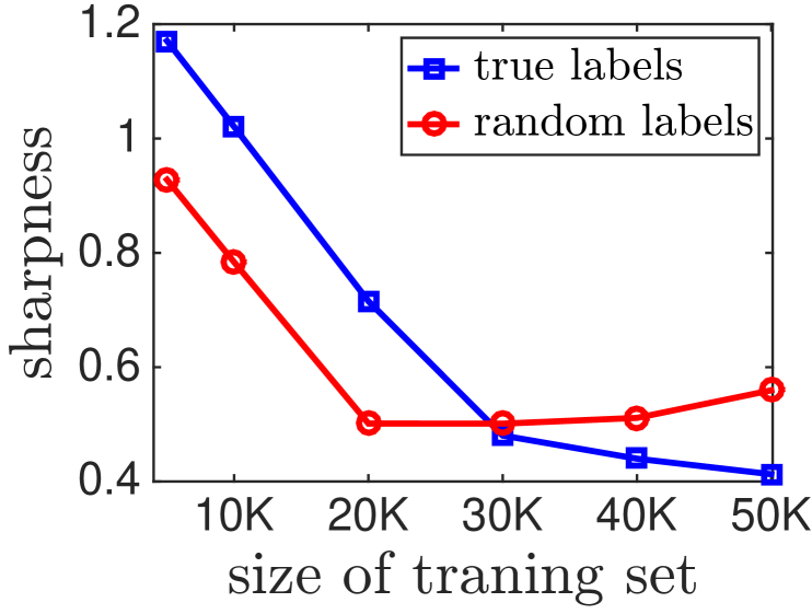
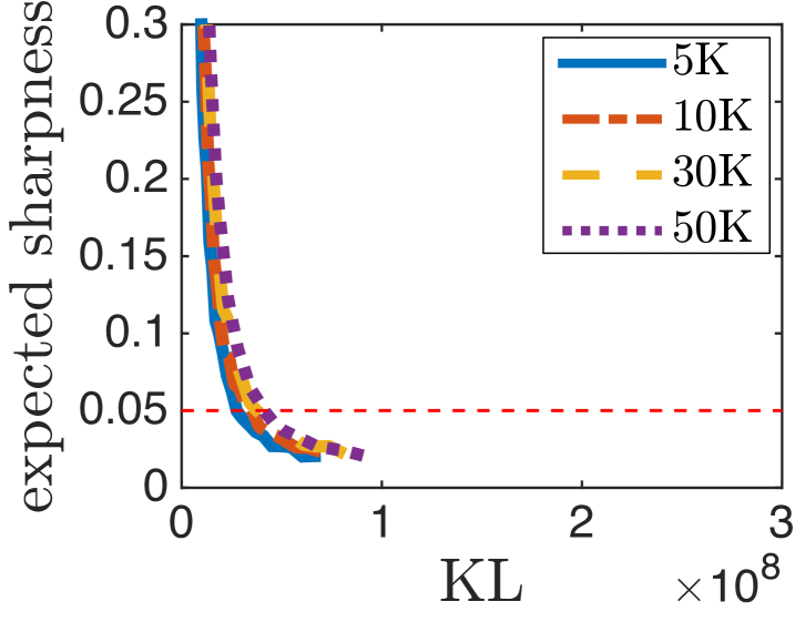
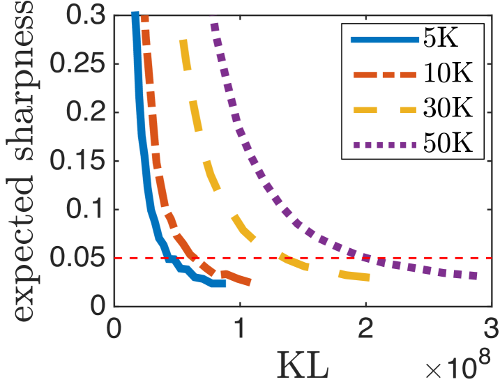
Figure 7.2: Sharpness and PAC-Bayes measures on a VGG network trained on subsets of CIFAR10 dataset with true or random labels. In the left panel, we plot max sharpness, which we calculate as suggested by keskar2016large where the perturbation for parameter $w_{i}$ has magnitude $5.10^{-4}({\left\lvert{w_{i}}\right\rvert}+1)$. The middle and right plots demonstrate the relationship between expected sharpness and KL divergence in PAC-Bayes analysis for true and random labels respectively. For PAC-Bayes plots, each point in the plot correspond to a choice of variable $\alpha$ where the standard deviation of the perturbation for the parameter $i$ is $\alpha(10{\left\lvert{w_{i}}\right\rvert}+1)$. The corresponding $KL$ to each $\alpha$ is nothing but weighted $\ell_{2}$ norm where the weight for each parameter is the inverse of the standard deviation of the perturbation.

7.4 Different Global Minima

Given different global minima of the training loss on the same training set and with the same model class, can these measures indicate which model is going to generalize better? In order to verify this property, we can calculate each measure on several different global minima and see if lower values of the measure imply lower generalization error. In order to find different global minima for the training loss, we design an experiment where we force the optimization methods to converge to different global minima with varying generalization abilities by forming a confusion set that includes samples with random labels. The optimization is done on the loss that includes examples from both the confusion set and the training set. Since deep learning models have very high capacity, the optimization over the union of confusion set and training set generally leads to a point with zero error over both confusion and training sets which thus is a global minima for the training set.

We randomly select a subset of CIFAR10 dataset with 10000 data points as the training set and our goal is to find networks that have zero error on this set but different generalization abilities on the test set. In order to do that, we train networks on the union of the training set with fixed size 10000 and confusion sets with varying sizes that consists of CIFAR10 samples with random labels; and we evaluate the learned model on an independent test set. The trained network achieves zero training error but as shown in Figure he test error of the model increases with increasing size of the confusion set. The middle panel of this Figure suggests that the norm of the learned networks can indeed be predictive of their generalization behavior. However, we again observe that sharpness has a poor behavior in these experiments. The right panel of this figure also suggests that PAC-Bayes measure of joint sharpness and KL divergence, has better behavior - for a fixed expected sharpness, networks that have higher generalization error, have higher norms.

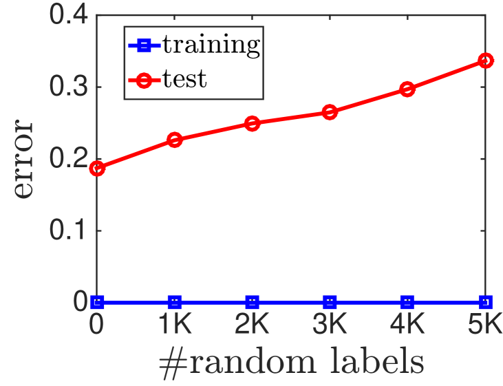
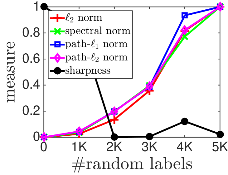
Figure 7.3: Experiments on global minima with poor generalization. For each experiment, a VGG network is trained on union of a subset of CIFAR10 dataset with size 10000 containing samples with true labels and another subset of CIFAR10 datasets with varying size containing random labels. The learned networks are all global minima for the objective function on the subset with true labels. The left plot indicates the training and test errors based on the size of the set with random labels. The plot in the middle shows change in different measures based on the size of the set with random labels. The plot on the right indicates the relationship between expected sharpness and KL in PAC-bayes for each of the experiments. Measures are calculated as explained in Figures d fig:cifar-core

7.5 Increasing Network Size

We also repeat the experiments conducted by neyshabur15b where a fully connected feedforward network is trained on MNIST dataset with varying number of hidden units and we check the values of different complexity measures on each of the learned networks.The left panel in Figure ows the training and test error for this experiment. While 32 hidden units are enough to fit the training data, we observe that networks with more hidden units generalize better. Since the optimization is done without any explicit regularization, the only possible explanation for this phenomenon is the implicit regularization by the optimization algorithm. Therefore, we expect a sensible complexity measure to decrease beyond 32 hidden units and behave similar to the test error. Different measures are reported for learned networks. The middle panel suggest that all margin/norm based complexity measures decrease for larger networks up to 128 hidden units. For networks with more hidden units, $\ell_{2}$ norm and $\ell_{1}$-path norm increase with the size of the network. The middle panel suggest that $\ell_{2}$-path norm can provide some explanation for this phenomenon. However, as we discussed in Section he actual complexity measure based on $\ell_{2}$-path norm also depends on the number of hidden units and taking this into account indicates that the measure based on $\ell_{2}$-path norm cannot explain this phenomenon. This is also the case for the margin based measure that depends on the spectral norm. In subsection discussed another complexity measure that also depends the spectral norm through Lipschitz continuity or robustness argument. Even though this bound is very loose, it is monotonic with respect to the spectral norm that is reported in the plots. Unfortunately, we do observe some increase in spectral norm by increasing number of hidden units beyond 512. The right panel shows that the joint PAC-Bayes measure decrease for larger networks up to size 128 but fails to explain this generalization behavior for larger networks. This suggests that the measures looked so far are not sufficient to explain all the generalization phenomenon observed in neural networks.

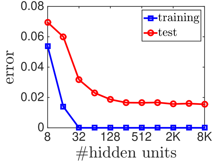
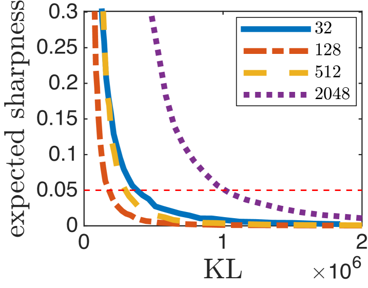
Figure 7.4: The generalization of two layer perceptron trained on MNIST dataset with varying number of hidden units. The left plot indicates the training and test errors. The test error decreases as the size increases. The middle plot shows different measures for each of the trained networks. The plot on the right indicates the relationship between expected sharpness and KL in PAC-Bayes for each of the experiments. Measures are calculated as explained in Figures d fig:hidden

Part II Geometry of Optimization and Generalization

Chapter 8 Invariances

In Chapter e discussed how optimization is related to generalization due to the implicit regularization. Revisiting the choice of gradient descent, we recall that optimization is also inherently tied to a choice of geometry or measure of distance, norm or divergence. Gradient descent for example is tied to the $\ell_{2}$ norm as it is the steepest descent with respect to $\ell_{2}$ norm in the parameter space, while coordinate descent corresponds to steepest descent with respect to the $\ell_{1}$ norm and exp-gradient (multiplicative weight) updates is tied to an entropic divergence. Moreover, at least when the objective function is convex, convergence behavior is tied to the corresponding norms or potentials. For example, with gradient descent, or SGD, convergence speeds depend on the $\ell_{2}$ norm of the optimum. The norm or divergence can be viewed as a regularizer for the updates. There is therefore also a strong link between regularization for optimization and regularization for learning: optimization may provide implicit regularization in terms of its corresponding geometry, and for ideal optimization performance the optimization geometry should be aligned with inductive bias driving the learning [srebro11].

Is the $\ell_{2}$ geometry on the weights the appropriate geometry for the space of deep networks? Or can we suggest a geometry with more desirable properties that would enable faster optimization and perhaps also better implicit regularization? As suggested above, this question is also linked to the choice of an appropriate regularizer for deep networks.

Focusing on networks with RELU activations in this section, we observe that scaling down the incoming edges to a hidden unit and scaling up the outgoing edges by the same factor yields an equivalent network computing the same function. Since predictions are invariant to such rescalings, it is natural to seek a geometry, and corresponding optimization method, that is similarly invariant. In this chapter, we study invariances in feedforward networks with shared weights.

8.1 Invariances in Feedforward and Recurrent Neural Networks

Feedforward networks are highly over-parameterized, i.e. there are many weight settings ${\mathbf{w}}$ that represent the same function $f_{\mathbf{w}}$. Since our true object of interest is the function $f$, and not the identity ${\mathbf{w}}$ of the weghts, it would be beneficial if optimization would depend only on $f_{\mathbf{w}}$ and not get “distracted” by difference in ${\mathbf{w}}$ that does not affect $f_{\mathbf{w}}$. It is therefore helpful to study the transformations on the weights that will not change the function presented by the network and come up with methods that their performance is not affected by such transformations.

Definition 1.

We say a class of neural networks is invariant to a transformation $\mathcal{T}$ if for any parameter setting $\mathbf{p}$ and its corresponding weights $\mathbf{w}$, $f_{\mathbf{w}}=f_{\mathcal{T}(\mathbf{w})}$. Similarly, we say an update rule $\mathcal{A}$ is invariant to $\mathcal{T}$ if for any $\mathbf{p}$ and its corresponding $\mathbf{w}$, $f_{\mathcal{A}(\mathbf{w})}=f_{\mathcal{A}(\mathcal{T}(\mathbf{w}))}$.

Invariances have also been studied as different mappings from the parameter space to the same function space [ollivier2015riemannian] while we define the transformation as a mapping inside a fixed parameter space. A very important invariance in feedforward networks is node-wise rescaling [neyshabur2016data]. For any internal node $v$ and any scalar $\alpha>0$, we can multiply all incoming weights into $v$ (i.e. $w_{u\rightarrow v}$ for any $(u\rightarrow v)\in E$) by $\alpha$ and all the outgoing weights (i.e. $w_{v\rightarrow u}$ for any $(v\rightarrow u)\in E$) by $1/\alpha$ without changing the function computed by the network. Not all node-wise rescaling transformations can be applied in feedforward nets with shared weights. This is due to the fact that some weights are forced to be equal and therefore, we are only allowed to change them by the same scaling factor.

Definition 2.

Given a class of neural networks, we say an invariant transformation $\mathcal{T}$ that is defined over edge weights is feasible for parameter mapping $\pi$ if the shared weights remain equal after the transformation, i.e. for any $i$ and for any $e,e^{\prime}\in E_{i}$, $\mathcal{T}(\mathbf{w})_{e}=\mathcal{T}(\mathbf{w})_{e^{\prime}}$.

We have discussed the complete characterize all feasible node-wise invariances of RNNs in [neyshabur2016path].

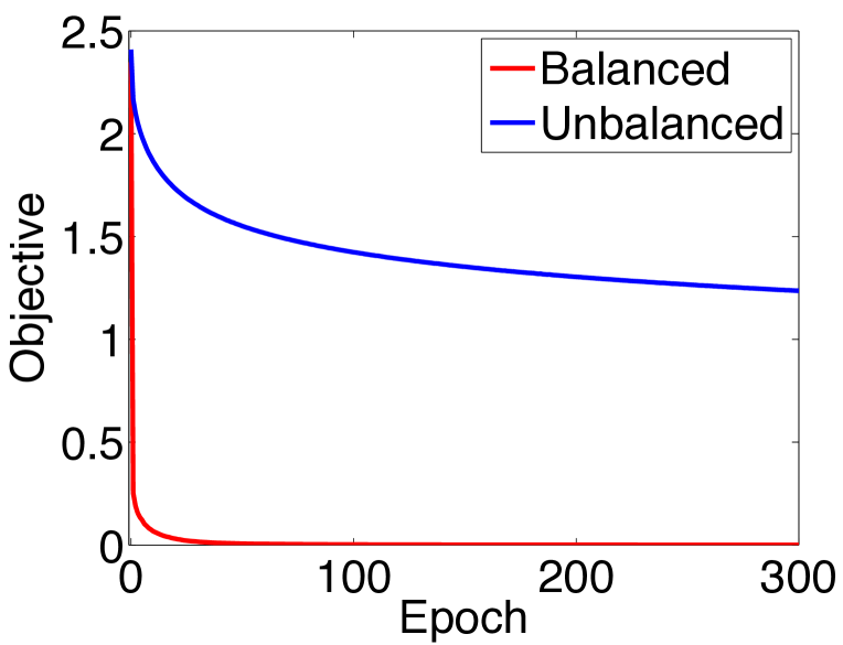
(a) Training on MNIST

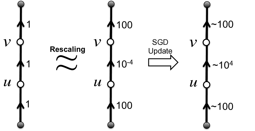
(b) Weight explosion in an unbalanced network

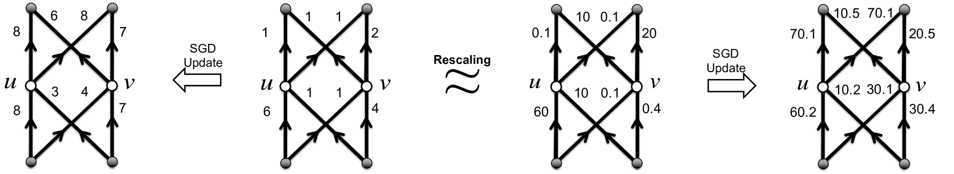
(c) Poor updates in an unbalanced network

Figure 8.1: (a): Evolution of the cross-entropy error function when training a feed-forward network on MNIST with two hidden layers, each containing 4000 hidden units. The unbalanced initialization (blue curve) is generated by applying a sequence of rescaling functions on the balanced initializations (red curve). (b): Updates for a simple case where the input is $x=1$, thresholds are set to zero (constant), the stepsize is 1, and the gradient with respect to output is $\delta=-1$. (c): Updated network for the case where the input is $x=(1,1)$, thresholds are set to zero (constant), the stepsize is 1, and the gradient with respect to output is $\delta=(-1,-1)$.

Unfortunately, gradient descent is not rescaling invariant. The main problem with the gradient updates is that scaling down the weights of an edge will also scale up the gradient which, as we see later, is exactly the opposite of what is expected from a rescaling invariant update.

Furthermore, gradient descent performs very poorly on “unbalanced” networks. We say that a network is balanced if the norm of incoming weights to different units are roughly the same or within a small range. For example, Figure shows a huge gap in the performance of SGD initialized with a randomly generated balanced network, when training on MNIST, compared to a network initialized with unbalanced weights. Here the unbalanced weights are generated by applying a sequence of random rescaling functions on the balanced weights to create a rescaling equivalent unbalanced network.

In an unbalanced network, gradient descent updates could blow up the smaller weights, while keeping the larger weights almost unchanged. This is illustrated in Figure . If this were the only issue, one could scale down all the weights after each update. However, in an unbalanced network, the relative changes in the weights are also very different compared to a balanced network. For example, Figure shows how two rescaling equivalent networks could end up computing a very different function after only a single update.

Therefore, it is helpful to understand what are the feasible node-wise rescalings for RNNs. In the following theorem, we characterize all feasible node-wise invariances in RNNs.

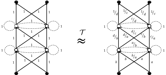
Figure 8.2: An example of invariances in an RNN with two hidden layers each of which has 2 hidden units. The dashed lines correspond to recurrent weights. The network on the left hand side is equivalent (i.e. represents the same function) to the network on the right for any nonzero $\alpha^{1}_{1}=a$, $\alpha^{1}_{2}=b$, $\alpha^{2}_{1}=c$, $\alpha^{2}_{2}=d$.

Theorem 26.

For any $\alpha$ such that $\alpha^{i}_{j}>0$, any Recurrent Neural Network with ReLU activation is invariant to the transformation $\mathcal{T}_{\alpha}\left(\left[\mathbf{W}_{\text{in}},\mathbf{W}_{\text{rec}},\mathbf{W}_{\text{out}}\right]\right)=\left[\mathcal{T}_{\text{in},\alpha}\left(\mathbf{W}_{\text{in}}\right),\mathcal{T}_{\text{rec},\alpha}\left(\mathbf{W}_{\text{rec}}\right),\mathcal{T}_{\text{out},\alpha}\left(\mathbf{W}_{\text{out}}\right)\right]$ where for any $i,j,k$:

$$\mathcal{T}_{\text{in},{\alpha}}(\mathbf{W}_{\text{in}})^{i}[j,k]=\begin{cases}\alpha^{i}_{j}\mathbf{W}_{\text{in}}^{i}[j,k]&i=1,\\ \left(\alpha^{i}_{j}/\alpha^{i-1}_{k}\right)\mathbf{W}_{\text{in}}^{i}[j,k]&1<i<d,\\ \end{cases}$$ (8.1.1)

$$\mathcal{T}_{\text{rec},\alpha}(\mathbf{W}_{\text{rec}})^{i}[j,k] =\left(\alpha^{i}_{j}/\alpha^{i}_{k}\right)\mathbf{W}_{\text{rec}}^{i}[j,k],\qquad\mathcal{T}_{\text{out},{\alpha}}(\mathbf{W}_{\text{out}})[j,k]=\left(1/\alpha^{d-1}_{k}\right)\mathbf{W}_{\text{out}}[j,k].$$

Furthermore, any feasible node-wise rescaling transformation can be presented in the above form.

The proof is given in Section he above theorem shows that there are many transformations under which RNNs represent the same function. An example of such invariances is shown in Fig. herefore, we would like to have optimization algorithms that are invariant to these transformations and in order to do so, we need to look at measures that are invariant to such mappings.

8.2 Understanding Invariances

The goal of this section is to discuss whether being invariant to node-wise rescaling transformations is sufficient or not.

Ideally we would like our algorithm to be at least invariant to all the transformations to which the model $G$ is invariant. Note that this is different than the invariances studied in [ollivier2015riemannian], in that they study algorithms that are invariant to reparametrizations of the same model but we look at transformations within the the parameter space that preserve the function in the model. This will eliminate the need for non-trivial initialization. Thus our goal is to characterize the whole variety of transformations to which the model is invariant and check if the algorithm is invariant to all of them.

We first need to note that invariance can be composed. If a network $G$ is invariant to transformations $T_{1}$ and $T_{2}$, it is also invariant to their composition $T_{1}\circ T_{2}$. This is also true for an algorithm. If an algorithm is invariant to transformations $T_{1}$ and $T_{2}$, it is also invariant to their composition. This is because $f_{T_{2}\circ T_{1}\circ\mathcal{A}(\mathbf{w})}=f_{T_{2}\circ\mathcal{A}(T_{1}\circ\mathbf{w})}=f_{\mathcal{A}(T_{2}\circ T_{1}(\mathbf{w}))}$.

Then it is natural to talk about the basis of invariances. The intuition is that although there are infinitely many transformations to which the model (or an algorithm) is invariant, they could be generated as compositions of finite number of transformations.

In fact, in the infinitesimal limit the directions of infinitesimal changes in the parameters to which the function $f_{\mathbf{w}}$ is insensitive form a subspace. This is because for a fixed input $\mathbf{x}$, we have

$$f_{\mathbf{w}+\bm{\Delta}}(x)=f_{\mathbf{w}}(\mathbf{x})+\sum\nolimits_{e\in E}\frac{\partial f_{\mathbf{w}}(\mathbf{x})}{\partial w_{e}}\cdot\Delta_{e}+O(\|\bm{\Delta}\|^{2}),$$ (8.2.1)

where $E$ is the set of edges, due to a Taylor expansion around $\mathbf{w}$. Thus the function $f_{\mathbf{w}}$ is insensitive (up to $O(\|\bm{\Delta}\|^{2})$) to any change in the direction $\bm{\Delta}$ that lies in the (right) null space of the Jacobian matrix $\partial f_{\mathbf{w}}(\mathbf{x})/\partial\mathbf{w}$ for all input $\mathbf{x}$ simultaneously. More formally, the subspace can be defined as

$$N(\mathbf{w})=\bigcap\nolimits_{\mathbf{x}\in\mathbb{R}^{|V_{\rm in}|}}\textrm{Null}\left(\frac{\partial f_{\mathbf{w}}(\mathbf{x})}{\partial\mathbf{w}}\right).$$ (8.2.2)

Again, any change to $\mathbf{w}$ in the direction $\bm{\Delta}$ that lies in $N(\mathbf{w})$ leaves the function $f_{\mathbf{w}}$ unchanged (up to $O(\|\bm{\Delta}\|^{2})$) at every input $x$. Therefore, if we can calculate the dimension of $N(\mathbf{w})$ and if we have ${\rm dim}N(\mathbf{w})=|V_{\rm internal}|$, where we denote the number of internal nodes by $|V_{\rm internal}|$, then we can conclude that all infinitesimal transformations to which the model is invariant can be spanned by infinitesimal node-wise rescaling transformations.

Note that the null space $N(\mathbf{w})$ and its dimension is a function of $\mathbf{w}$. Therefore, there are some points in the parameter space that have more invariances than other points. For example, suppose that $v$ is an internal node with ReLU activation that receives connections only from other ReLU units (or any unit whose output is nonnegative). If all the incoming weights to $v$ are negative including the bias, the output of node $v$ will be zero regardless of the input, and the function $f_{\mathbf{w}}$ will be insensitive to any transformation to the outgoing weights of $v$. Nevertheless we conjecture that as the network size grows, the chance of being in such a degenerate configuration during training will diminish exponentially.

When we study the dimension of $N(\mathbf{w})$, it is convenient to analyze the dimension of the span of the row vectors of the Jacobian matrix $\partial f_{\mathbf{w}}(\mathbf{x})/\partial\mathbf{w}$ instead. We define the degrees of freedom of model $G$ at $\mathbf{w}$ as

$$d_{G}(\mathbf{w})={\rm dim}\left(\bigcup\nolimits_{\mathbf{x}\in\mathbb{R}^{|V_{\rm in}|}}{\rm Span}\left(\frac{\partial f_{\mathbf{w}}(\mathbf{x})}{\partial\mathbf{w}}[v,:]:v\in V_{\rm out}\right)\right),$$ (8.2.3)

where $\partial f_{\mathbf{w}}(\mathbf{x})[v,:]/\partial\mathbf{w}$ denotes the $v$th row vector of the Jacobian matrix and $\mathbf{x}$ runs over all possible input $\mathbf{x}$. Intuitively, $d_{G}(\mathbf{w})$ is the dimension of the set of directions that changes $f_{\mathbf{w}}(x)$ for at least one input $x$.

Due to the rank nullity theorem $d_{G}(\mathbf{w})$ and the dimension of $N(\mathbf{w})$ are related as follows:

$$d_{G}(\mathbf{w})+{\rm dim}\left(N(\mathbf{w})\right)=|E|,$$

where $|E|$ is the number of parameters. Therefore, again if $d_{G}(\mathbf{w})=|E|-|V_{\rm internal}|$, then we can conclude that infinitesimally speaking, all transformations to which the model is invariant can be spanned by node-wise rescaling transformations.

Considering only invariances that hold uniformly over all input $\mathbf{x}$ could give an under-estimate of the class of invariances, i.e., there might be some invariances that hold for many input $\mathbf{x}$ but not all. An alternative approach for characterizing invariances is to define a measure of distance between functions that the neural network model represents based on the input distribution, and infinitesimally study the subspace of directions to which the distance is insensitive. We can define distance between two functions $f$ and $g$ as

$$D(f,g)={\mathbb{E}\left[{\mathbf{x}\sim\mathcal{D}}\right]}\left[m(f(\mathbf{x}),g(\mathbf{x}))\right],$$

where $m:\mathbb{R}^{|V_{\rm out}|\times|V_{\rm out}|}\rightarrow\mathbb{R}$ is a (possibly asymmetric) distance measure between two vectors $\mathbf{z},\mathbf{z}^{\prime}\in\mathbb{R}^{|V_{\rm out}|}$, which we require that $m(\mathbf{z},\mathbf{z})=0$ and $\partial m/\partial\mathbf{z}^{\prime}_{\mathbf{z}=\mathbf{z}^{\prime}}=0$. For example, $m(\mathbf{z},\mathbf{z}^{\prime})=\|\mathbf{z}-\mathbf{z}^{\prime}\|^{2}$.

The second-order Taylor expansion of the distance $D$ can be written as

$$D(f_{\mathbf{w}}\|f_{\mathbf{w}+\bm{\Delta}}) =\frac{1}{2}\bm{\Delta}^{\top}\cdot F(\mathbf{w})\cdot\bm{\Delta}+o(\|\bm{\Delta}\|^{2}),$$

where

$$F(\mathbf{w}) ={\mathbb{E}\left[{\mathbf{x}\sim\mathcal{D}}\right]}\left[\left(\frac{\partial f_{\mathbf{w}}(\mathbf{x})}{\partial\mathbf{w}}\right)^{\top}\cdot\left.\frac{\partial^{2}m(\mathbf{z},\mathbf{z}^{\prime})}{\partial\mathbf{z}^{\prime 2}}\right|_{\mathbf{z}=\mathbf{z}^{\prime}=f_{\mathbf{w}}(\mathbf{x})}\cdot\left(\frac{\partial f_{\mathbf{w}}(\mathbf{x})}{\partial\mathbf{w}}\right)\right]$$

and $\partial^{2}m(\mathbf{z},\mathbf{z}^{\prime})/\partial\mathbf{z}^{\prime 2}|_{\mathbf{z}=\mathbf{z}^{\prime}=f_{\mathbf{w}}(\mathbf{x})}$ is the Hessian of the distance measure $m$ at $\mathbf{z}=\mathbf{z}^{\prime}=f_{\mathbf{w}}(\mathbf{x})$.

Using the above expression, we can define the input distribution dependent version of $N(\mathbf{w})$ and $d_{G}(\mathbf{w})$ as

$$N_{\mathcal{D}}(\mathbf{w})={\rm Null}F(\mathbf{w}),\qquad d_{G,\mathcal{D}}(\mathbf{w})={\rm rank}F(\mathbf{w}).$$

Again due to the rank-nullity theorem we have $d_{G,\mathcal{D}}(\mathbf{w})+{\rm dim}(N_{\mathcal{D}}(\mathbf{w}))=|E|$.

As a special case, we obtain the Kullback-Leibler divergence $D_{\rm KL}$, which is commonly considered as the way to study invariances, by choosing $m$ as the conditional Kullback-Leibler divergence of output $y$ given the network output as

$$m(\mathbf{z},\mathbf{z}^{\prime})={\mathbb{E}\left[{y\sim q(y|\mathbf{z})}\right]}\left[\log\frac{q(y|\mathbf{z})}{q(y|\mathbf{z}^{\prime})}\right],$$

where $q(y|\mathbf{z})$ is a link function, which can be, e.g., the soft-max $q(y|\mathbf{z})=e^{z_{y}}/\sum_{y^{\prime}=1}^{|V_{\rm out}|}e^{z_{y^{\prime}}}$. However, note that the invariances in terms of $D_{\rm KL}$ depends not only on the input distribution but also on the choice of the link function $q(y|\mathbf{z})$.

8.2.1 Path-based characterization of the network

A major challenge in studying the degrees of freedom (8.2.3) is the fact that the Jacobian $\partial f_{\mathbf{w}}(x)/\partial\mathbf{w}$ depends on both parameter $w$ and input $x$. In this section, we first tease apart the two dependencies by rewriting $f_{\mathbf{w}}(x)$ as the sum over all directed paths from every input node to each output node as follows:

$$f_{\mathbf{w}}(\mathbf{x})[v] =\sum\nolimits_{p\in\Pi(v)}g_{p}(\mathbf{x})\cdot\pi_{p}(\mathbf{w})\cdot x[{\rm head}(p)],$$ (8.2.4)

where $\Pi(v)$ is the set of all directed path from any input node to $v$, ${\rm head}(p)$ is the first node of path $p$, $g_{p}(\mathbf{x})$ takes 1 if all the rectified linear units along path $p$ is active and zero otherwise, and $\pi_{p}(\mathbf{w})=\prod_{e\in E(p)}w(e)$ is the product of the weights along path $p$; $E(p)$ denotes the set of edges that appear along path $p$.

Let $\Pi=\cup_{v\in V_{\rm out}}\Pi(v)$ be the set of all directed paths. We define the path-Jacobian matrix $J(\mathbf{w})\in\mathbb{R}^{|\Pi|\times|E|}$ as $J(\mathbf{w})=(\partial\pi_{p}(\mathbf{w})/\partial w_{e})_{p\in\Pi,e\in E}$. In addition, we define $\bm{\phi}(\mathbf{x})$ as a $|\Pi|$ dimensional vector with $g_{p}(\mathbf{x})\cdot x[{\rm head}(p)]$ in the corresponding entry. The Jacobian of the network $f_{\mathbf{w}}(\mathbf{x})$ can now be expressed as

$$\frac{\partial f_{\mathbf{w}}(\mathbf{x})[v]}{\partial\mathbf{w}} =J_{v}(\mathbf{w})^{\top}\bm{\phi}_{v}(\mathbf{x}),$$ (8.2.5)

where where $J_{v}(\mathbf{w})$ and $\bm{\phi}_{v}(\mathbf{x})$ are the submatrix (or subvector) of $J(\mathbf{w})$ and $\bm{\phi}(\mathbf{x})$ that corresponds to output node $v$, respectively. Expression (8.2.5) clearly separates the dependence to the parameters $\mathbf{w}$ and input $\mathbf{x}$.

Now we have the following statement (the proof is given in Section theorem The degrees-of-freedom $d_G(w)$ of neural network model $G$ is at most the rank of the path Jacobian matrix $J(w)$. The equality holds if $dim(Span(ϕ(x):x∈R^|V_in|))=|Π|$; i.e. when the dimension of the space spanned by $ϕ(x)$ equals the total number of paths $|Π|$.

An analogous statement holds for the input distribution dependent degrees of freedom $d_G,D(w)$, namely, $d_G,D(w)≤rank J(w)$ and the equality holds if the rank of the $|Π|×|Π|$ path covariance matrix $(E[x∼D][ ∂^2 m(z,z')/∂z'_v∂z'_v'ϕ_p(x)ϕ_p'(x) ])_p,p'∈Π$ is full, where $v$ and $v'$ are the end nodes of paths $p$ and $p'$, respectively.

It remains to be understood when the dimension of the span of the path vectors $ϕ(x)$ become full. The answer depends on $w$. Unfortunately, there is no typical behavior as we know from the example of an internal ReLU unit connected to ReLU units by negative weights. In fact, we can choose any number of internal units in the network to be in this degenerate state creating different degrees of degeneracy. Another way to introduce degeneracy is to insert a linear layer in the network. This will superficially increase the number of paths but will not increase the dimension of the span of $ϕ(x)$. For example, consider a linear classifier $z_out=⟨w, x ⟩$ with $|V_in|$ inputs. If the whole input space is spanned by $x$, the dimension of the span of $ϕ(x)$ is $|V_in|$, which agrees with the number of paths. Now let's insert a linear layer with units $V_1$ in between the input and the output layers. The number of paths has increased from $|V_in|$ to $|V_in|⋅|V_1|$. However the dimension of the span of $ϕ(x)=→1_|V_1|⊗x$ is still $|V_in|$, because the linear units are always active. Nevertheless we conjecture that there is a configuration $w$ such that $dim(Span(ϕ(x):x∈R^|V_in|))=|Π|$ and the set of such $w$ grows as the network becomes larger.

8.2.2 Combinatorial characterization of the rank of path Jacobian

Finally, we show that the rank of the path-Jacobian matrix $J(w)$ is determined purely combinatorially by the graph $G$ except a subset of the parameter space with zero Lebesgue measure. The proof is given in Section~theorem The rank of the path Jacobian matrix $J(w)$ is generically (excluding set of parameters with zero Lebesgue measure) equal to the number of parameters $|E|$ minus the number of internal nodes of the network.