Edge states in a ferromagnetic honeycomb lattice with armchair boundaries

Abstract

We investigate the properties of magnon edge states in a ferromagnetic honeycomb lattice with armchair boundaries. In contrast with fermionic graphene, we find novel edge states due to the missing bonds along the boundary sites. After introducing an external on-site potential at the outermost sites we find that the energy spectra of the edge states are tunable. Additionally, when a non-trivial gap is induced, we find that some of the edge states are topologically protected and also tunable. Our results may explain the origin of the novel edge states recently observed in photonic lattices. We also discuss the behavior of these edge states for further experimental confirmations.

Introduction.— One intriguing aspect of electrons moving in finite-sized honeycomb lattices is the presence of edge states, which have strong implications in the electronic properties and play an essential role in the electronic transport Fujita et al. (1996); Nakada et al. (1996); Kohmoto and Hasegawa (2007). It is well known that natural graphene exhibits edge states under some particular boundaries Akabayashi et al. (2010); Delplace et al. (2011). For example, there are flat edge states connecting the two Dirac points in a lattice with zig-zag Fujita et al. (1996) or bearded edges Klein (1994). On the contrary, there are no edge states in a lattice with armchair boundary Zhao et al. (2012), unless a boundary potential is applied Chiu and Chu (2012).

The edge states have also been studied in magnetic insulators Fujimoto (2009); Onose et al. (2010); Cao et al. (2015), where the spin moments are carried by magnons. Recently, it has been shown that the magnonic equivalence for the Kane-Mele-Haldane model is a ferromagnetic Heisenberg Hamiltonian with the Dzialozinskii-Moriya interaction Owerre (2016); Kim et al. (2016). Firstly, while the energy band structure of the magnons of ferromagnets on the honeycomb lattice closely resembles that of the fermionic graphene Pantaleón and Xian (2017); Sakaguchi and Matsumoto (2016), it is not clear whether or not they show similar edge states, particularly in view of the interaction terms in the bosonic models which are usually ignored in graphene Lado et al. (2015). Secondly, most recent experiments in photonic lattices have observed novel edge states in honeycomb lattices with bearded Plotnik et al. (2014) and armchair Milićević et al. (2017) boundaries, which are not present in fermionic graphene. The main purpose of this paper is to address these two issues. By considering a ferromagnetic honeycomb lattice with armchair boundaries, we find that the bosonic nature of the Hamiltonian reveals novel edge states which are not present in their fermionic counterpart. After introducing an external on-site potential at the outermost sites, we find that the edge states are tunable. Interestingly, we find that the nature of such edge states is Tamm-like Tamm (1932), in contrast with the equivalent model for the armchair graphene Chiu and Chu (2012) but, as mentioned earlier, in agreement with the experiments in photonic lattices Plotnik et al. (2014); Milićević et al. (2017). Furthermore, after introducing a Dzialozinskii-Moriya interaction (DMI), we find that the topologically protected edge states are sensitive to the presence of the Tamm-like states and they also become tunable.

Model.— We consider the following Hamiltonian for a ferromagnetic honeycomb lattice,

$$H=-J\sum_{\left\langle i,j\right\rangle}\mathbf{S}_{i}\cdot\mathbf{S}_{j}+\sum_{\left\langle\left\langle i,j\right\rangle\right\rangle}\bm{D}_{ij}\cdot\left(\mathbf{S}_{i}\times\mathbf{S}_{j}\right),$$ (1)

where the first summation runs over the nearest-neighbors (NN) and the second over the next-nearest-neighbors (NNN), $J\left(>0\right)$ is the isotropic ferromagnetic coupling, $\bm{S}_{i}$ is the spin moment at site $i$ and $\bm{D}_{ij}$ is the DMI vector between NNN sites Moriya (1960). If we assume that the lattice is at the $x$-$y$ plane, according to Moriya’s rules Moriya (1960), the DMI vector vanishes for the NN but has non-zero component along the $z$ direction for the NNN. Hence, we can assume $\bm{D}_{ij}=D\nu_{ij}\hat{z}$, where $\nu_{ij}=\pm 1$ is an orientation dependent coefficient in analogy with the Kane-Mele model Kane and Mele (2005). For the infinite system in the linear spin-wave approximation (LSWA), the Hamiltonian in Eq. (1) can be reduced to a bosonic equivalent of the Kane-Mele-Haldane model Owerre (2016); Kim et al. (2016); Pantaleón and Xian (2017). To investigate the edge states we consider an armchair boundary along the $x$ direction, with a large $N$ sites in the $y$ direction, as shown in Fig. (1). A partial Fourier transform is made and the Hamiltonian given in Eq. (1) in LSWA can be written in the form,

$$H=-t\sum_{k}\Psi_{k}^{\dagger}M\Psi_{k},$$ (2)

where $\Psi_{k}^{\dagger}=\left[\Psi_{k,A}^{\dagger},\,\Psi_{k,B}^{\dagger}\right]$ is a $2N\times 2N$, $2$-component spinor, $k$ is the Bloch wave number in the $x$ direction and $t=JS$. The matrix elements of $M$ are $N\times N$ matrices given by: $M_{11}=\left(1-\delta_{1}\right)T^{\dagger}T+\left(1-\delta_{N}\right)TT^{\dagger}+\left(1+\delta_{1}+\delta_{N}\right)I+M_{D}$, $M_{12}=-J_{1}I-J_{2}\left(T+T^{\dagger}\right)$, $M_{21}=M_{12}^{\dagger}$, $M_{22}=M_{11}-2M_{D}$ and $M_{D}=J_{3}\left(TT-T^{\dagger}T^{\dagger}\right)+J_{4}\left(T+T^{\dagger}\right)$ the DMI contribution. Here, $T$ is a displacement matrix as defined in Ref. You et al. (2008) and $I$ a $N\times N$ identity matrix. We have also introduced two on-site energies $\delta_{1}$ and $\delta_{N}$ at the outermost sites of each boundary, respectively. The coupling terms are: $J_{1}=e^{-ik}$, $J_{2}=e^{\frac{1}{2}ik}$, $J_{3}=i\,D^{\prime}$, $J_{4}=2i\,D^{\prime}\,\cos\left(3k/2\right)$ and $D^{\prime}=D/J$. The numerical diagonalization of the matrix given by Eq. (2) reveals that the bulk spectra is gapless only if $N=3m+1$, with $m$ a positive integer Wang et al. (2016). However, to avoid size-dependent bulk gaps or hybridization between edge states of opposite edges Chiu and Chu (2012), we consider a large $N$ where the edge states are independent of the size Hatsugai (1993a, b).

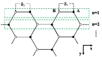
Figure 1: Squematics of the upper armchair edge of a honeycomb lattice. The external on-site potential $\delta_{1}$ is applied at the outermost sites. Here, $n$ is a real-space row index in $y$ direction perpendicular to the edge. For a large $N$, we consider the opposite edge with the same structure and with an on-site potential $\delta_{N}$.

Boundary conditions.— From the explicit form of the matrix elements in Eq. (2), the coupled Harper equations can be obtained Harper (1955). If we assume that the edge states are exponentially decaying from the armchair boundary, we can consider the following anzats König et al. (2008); Wang et al. (2009) for the eigenstates of $M$ in Eq. (2),

$$\Psi_{k}\left(n\right)=\left[\begin{array}[]{c}\psi_{k,A}\left(n\right)\\ \psi_{k,B}\left(n\right)\end{array}\right]=z^{n}\left[\begin{array}[]{c}\phi_{k,A}\\ \phi_{k,B}\end{array}\right],$$ (3)

where $\left[\phi_{k,A},\,\phi_{k,B}\right]^{t}$ is an eigenvector of $M$, $z$ is a complex number and $n\,\left\{=1,\,2,\,3\,...\right\}$ is a real space lattice index in the $y$ direction, as shown in Fig. (1). Upon substitution of the anzats in the coupled Harper equations, the complex number $z$ obey the following polynomial equation,

$$\sum_{\mu=0}^{4}a_{\mu}(z+z^{-1})^{\mu}=0,$$ (4)

with coefficients: $a_{0}=1-\left(3-\varepsilon\right)^{2}-4J_{4}^{2}$, $a_{1}=8J_{3}J_{4}+J_{1}^{\ast}J_{2}+J_{2}^{\ast}J_{1}$, $a_{2}=-4J_{3}^{2}+J_{4}^{2}+1$, $a_{3}=-2J_{3}J_{4}$ and $a_{4}=J_{3}^{2}$. For a given $k$ and energy $\varepsilon$, such a polynomial always yields four solutions for $\left(z+z^{-1}\right)$. Since we require a decaying wave from the boundary, only the solutions with $\left|z\right|<1$ are relevant for the description of the edge states at the upper edge and $\left|z\right|>1$ for the lower (opposite) edge. The eigenfunction of Eq. (2) satisfying $\underset{n\rightarrow\infty}{lim}\,\Psi_{k}\left(n\right)=0$ may now in general be written as,

$$\psi_{k,l}\left(n\right)=\sum_{\upsilon=1}^{4}c_{v}z_{v}^{n}\phi_{l,v},$$ (5)

where the coefficients $c_{\upsilon}$ are determined by the boundary conditions and $\phi_{l,v}$ is the two-component eigenvector $\left(l=A,\,B\right)$ of $M$. From the Harper equations provided by the Eq. (2) and Eq. (3), the boundary conditions are satisfied by,

$$\left(1-\delta_{1}\right)\psi_{k,A}\left(1\right)-J_{2}\psi_{k,B}\left(0\right) =0,$$ (6)

$$\left(1-\delta_{1}\right)\psi_{k,B}\left(1\right)-J_{2}^{\ast}\psi_{k,A}\left(0\right) =0,$$ (7)

$$J_{4}\psi_{k,A}\left(0\right)-J_{3}\psi_{k,A}\left(-1\right) =0,$$ (8)

$$J_{4}\psi_{k,B}\left(0\right)-J_{3}\psi_{k,B}\left(-1\right) =0.$$ (9)

By Eq. (5), the above relations can be written as a set of equations for the unknown coefficients $c_{v}$. The non-trivial solution and the polynomial given by Eq. (4), provide us a complete set of equations for the edge state energy dispersion and they can be solved numerically. The same procedure can be followed to obtain the solutions for the opposite edge.

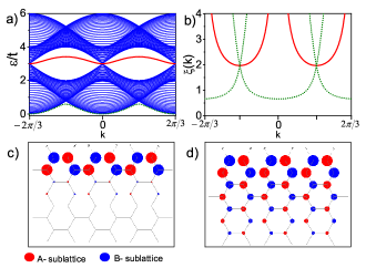
Figure 2: (Color online) a) Edge state energy dispersion for $D=0$ and $\delta_{1}=\delta_{N}=0$. The blue regions are the bulk energy spectra. The green (dotted) and red (continuous) lines are the edge state energy bands. In b) their corresponding penetration lengths are shown. The magnon density profile for the edge magnon is shown in c) for $\varepsilon=\left(2\pm\sqrt{2}\right)t$ at $k=\pm\pi/3$, and in d) for $\varepsilon=0.298\,t$ at $k=\pm 0.65$. The radius of each circle is proportional to the magnon density.

Zero DMI.— For the system without DMI, the coupling terms invoving $J_{3}$ and $J_{4}$ vanish, and the boundary conditions are reduced to the Eqs. (6) and (7) with a quadratic polynomial in $(z+z^{-1})$ of Eq. (4). In particular, for the (uniform) case with $\delta_{1}=\delta_{N}=1$, the edge and the bulk sites have the same on-site potential and the boundary conditions provide us with two bulk solutions with $z^{2}=1$. Therefore, in analogy with graphene with armchair edges, there are not edge states Zhao et al. (2012). However, as shown in Fig. (2a), in the absence of external on-site potential $\left(\delta_{1}=\delta_{N}=0\right)$, two new dispersive localized modes are obtained. Located between (red, continuous line) and below (green, dotted) the bulk bands, such edge states are well defined along the Brillouin zone and their energy bands are doubly degenerated due to the fact that there are two edges in the ribbon.

These edge states have not been previously predicted or observed in magnetic insulators. However, we believe that they are analogous to the novel edge states recently observed in a photonic honeycomb lattice with armchair edges Milićević et al. (2017). Although in Ref. Milićević et al. (2017) these edge states may be attributed to the dangling bonds along the boundary sites (the details have been given for zig-zag and bearded but not for armchair edges), and since these dangling bonds can be viewed as effective defects along the edges, similar physics is contained in our model where the effective defects are described by the different on-site potential at the boundaries. We believe that our approach has the advantage of simple implementation for various boundary conditions. In particular, we have obtained analytical expressions for the wavefunctions and their confinement along the boundary. The latter is given by the penetration length (or width) of the edge state Doh and Jeon (2013) defined as,

$$\xi_{i}\left(k\right)\equiv\frac{\sqrt{3}}{2}\left[\ln\left|\frac{1}{z_{i}\left(k\right)}\right|\right]^{-1},$$ (10)

indicating a decay of the form $\sim e^{-y/\xi_{i}\left(k\right)}$. In the above equation, $z_{i}$ is the $i$-th decaying factor in the linear combination, Eq. (5). Since we require two decaying factors to construct the edge state, we have two penetration lengths as mentioned in Ref. Milićević et al. (2017). The penetration lengths for the edge states with $\delta_{1}=\delta_{N}=0$ are shown in the Fig. (2b). The dotted (green) and continuous (red) lines are the corresponding penetration lengths for the edge states in the Fig. (2a). The edge state between the bulk bands (red, continuous) is composed by two penetration lengths but they are indistinguishable to each other. This indicates that the decaying factors are complex conjugates to each other, $z_{1}=z_{2}^{\ast}$ Doh and Jeon (2013); Pantaleón and Xian (2017). The edge state below the lower bulk band (green, dotted) depends on two penetration lengths in the region around $k=\pm\pi/3$. However, outside such region, one penetration length diverges, $\left|z\right|\rightarrow 1$, while the other one decreases to a minimum value. This means that the edge state tends to merge with the bulk and is almost indistinguishable at $k=0,\,\pm 2\pi/3$. Furthermore, as we can see in the Fig. (2b), at $k=\pm\pi/3$, the penetration length of both edge states is identical hence they have their maximum confinement along the boundary at the same Bloch wave-vector. This is shown in the Fig. (2c) where we plot the magnon density, $\left|\psi_{k,l}\left(n\right)/\psi_{k,l}\left(1\right)\right|^{2}$, for both edge states at $k=\pm\pi/3$ with their corresponding energies, $\varepsilon=\left(2\pm\sqrt{2}\right)t$. In addition, in the Fig. (2d) the magnon density for the edge state below the lower bulk band with energy $\varepsilon=0.298\,t$ at $k=\pm 0.65$ is shown, where as we mentioned before, the edge state tends to spread to the inner sites.

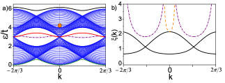
Figure 3: (Color online) (Color online) a) Edge state energy dispersion for $D=0$ with $\delta_{1}=2.5$ and $\delta_{N}=0$. The blue regions are the bulk energy spectra. The dotted (green) and continuous (red) lines are the edge state energy bands at the lower edge. The dot-dashed (purple) line, continuous (black) line and the circle (orange) are the edge states at the upper edge. In b) the penetration lengths of the corresponding edge states at the upper edge is shown.

The edge states discussed above have been obtained with no gap in the bulk and their dispersion relations are between the Dirac points. Their existence without external on-site potentials indicates that the edge states are “Tamm-like” Tamm (1932); Plotnik et al. (2014). Such type of states are usually associated with surface perturbations or defects. However, in our system no defects are present. The nature of such edge states can be explained in terms of the intrinsic on-site potential, where each site along the armchair boundary has two nearest-neighbors and the intrinsic on-site potential is lower than in the bulk. Such a difference plays the same role as an effective defect which allows the existence of a Tamm-like state.

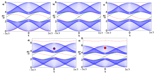
Figure 4: (Color online) Edge state energy dispersion for $D=0.1\,J$. The blue regions are the bulk energy spectra. For $\delta_{N}=1$ (lower edge) there is an edge state crossing the gap (green, continuous). The red (dotted) lines are the edge states for a) $\delta_{1}=0$, b) $\delta_{1}=1$, c) $\delta_{1}=2$, d) $\delta_{1}=3$ and e) $\delta_{1}=4$. The circles in d) and e) are edge states within the bulk energy bands.

We next discuss the effects of edge potentials. It has been shown that edge states can be induced by edge potentials in the armchair graphene Chiu and Chu (2012), however, the edge states that we found are a consequence of the bosonic nature of the lattice as discussed above. Since they exist without opening a gap and they are dispersive, it is not clear if they can be predicted by a topological approach. Our approach reveals that the edge states in a bosonic lattice are strongly dependent on the on-site potential along the boundary. For example, if $\delta_{1}=2.5$ (with $\delta_{N}=0$) some new features are obtained. As shown in Fig. (3a), the presence of the strong external on-site potential reveals three edge states at the upper boundary: a high energy edge state over the bulk bands (black, continuous line), an edge state between the bulk bands (purple, dot-dashed line), and interestingly, an edge state within the bulk bands (orange circle). Such edge state is strongly localized and is highly dispersive. It merges into the bulk with an small change in their Bloch wave-number and may be difficult to detect in a magnetic insulator. It is therefore very encouraging that similar edge state was observed in a photonic lattice Milićević et al. (2017). The penetration lengths of the corresponding edge states are shown in the Fig. (3b), firstly, the edge state over the bulk bands (black, continuous line) depends on two decaying factors and the oscillating behavior of their corresponding penetration lengths reveals that is strongly localized along the boundary sites and it never merges into the bulk. Secondly, the edge state within the bulk bands (orange, dashed line) depends on a single decaying factor and is highly dispersive. Thirdly, the edge state between the bulk bands (purple, dot-dashed) depends on a single penetration length since the two decaying factors are conjugate to each other Doh and Jeon (2013).

Non-zero DMI.— It is well known that a non-zero DMI in a bosonic honeycomb lattice makes the band structure topologically non-trivial and reveals metallic edge states which transverse the gap Owerre (2016). However, the edge states that appear, under, within and over the bulk bands in Fig. (2a) and Fig. (3a) are distinct to the edge states predicted by topological arguments.

In the Fig. (4) we show the energy bands for a DMI strength of $D=0.1\,J$, where we keep a fixed $\delta_{N}=1$ and we modified $\delta_{1}$. The continuous (green) line that cross the gap from the lower to the upper bulk bands is the edge state at the lower edge. The dotted (red) lines correspond to the edge states at the upper edge. If we follow the edge state energy spectra at the upper boundary from the Fig. (4a) to the Fig. (4c), we observe that the edge state within the bulk gap change its concavity. The Tamm-like state below the bulk bands, Fig. (4a), merge with the bulk and a new Tamm-like state appears at the top of the upper bulk band, as shown in Fig. (4c). If we keep increasing the value of the external on-site potential the Tamm-like state over the bulk band in Fig. (4c) moves away from the upper bulk band, Fig. (4d). Furthermore, a second Tamm-like state appears with components within the bulk, as shown in Fig. (4d) and Fig. (4e). The boundary conditions suggest that the existence of these two tunable edge states is due to the two sites in the unit cell of the armchair boundary and, by symmetry, the same behavior is expected at the opposite edge. These edge states can be made to locate below, within and over the bulk bands. If a non-trivial gap is induced the topologically protected edge states are also tunable.

Finally, a similar phenomena is expected for a lattice with zig-zag or bearded boundaries. In both cases there is a single outermost site and Tamm-like edge states may appear due to the missing bond and/or by the external on-site potential. Since the outermost site at the lattice with a bearded boundary has three missing bonds, the effective defect should be stronger than the corresponding to a zig-zag boundary. This may be related with the existence of the “unconventional” edge states found in optical lattices Plotnik et al. (2014). A more extensive investigation of Tamm-like edge states along different boundaries will be reported elsewhere.

Conclusions.— We have analyzed the edge states in a ferromagnetic honeycomb lattice with armchair edges and an external on-site potential at the outermost sites. In contrast with graphene, our system without external on-site potential reveals two edge states. It is clear that the open boundary in a bosonic lattice creates an effective defect by a difference in the on-site potential between the bulk and boundary sites. This effective defect is responsible for the existence of the novel edge states. By introducing an external on-site potential at the outermost sites we found that the nature of this edge states is Tamm-like. We also found that these edge states are tunable in their shapes and positions depending on the external on-site potential strength. Such tunability can be used to modify the topologically protected edge states when a non-trivial gap is induced. Finally, we found that the number of these tunable edge states is related to the number of sites in a unit cell along the boundary. We believe that our results may explain the edge states recently found in optical lattices Plotnik et al. (2014); Milićević et al. (2017) and motivate new experiments in both magnonic and photonic lattices.

Pierre. A. Pantaleón is sponsored by Mexico’s National Council of Science and Technology (CONACYT) under the scholarship 381939.

References

- Fujita et al. (1996) M. Fujita, K. Wakabayashi, K. Nakada, and K. Kusakabe, J. Phys. Soc. Japan 65, 1920 (1996).
- Nakada et al. (1996) K. Nakada, M. Fujita, G. Dresselhaus, and M. S. Dresselhaus, Phys. Rev. B 54, 17954 (1996).
- Kohmoto and Hasegawa (2007) M. Kohmoto and Y. Hasegawa, Phys. Rev. B 76, 205402 (2007).
- Akabayashi et al. (2010) K. W. Akabayashi, S. O. Kada, R. T. Omita, S. F. Ujimoto, Y. N. Atsume, K. Wakabayashi, S. Okada, R. Tomita, S. Fujimoto, and Y. Natsume, J. Phys. Soc. Japan 79, 034706 (2010).
- Delplace et al. (2011) P. Delplace, D. Ullmo, and G. Montambaux, Phys. Rev. B 84, 195452 (2011).
- Klein (1994) D. Klein, Chem. Phys. Lett. 217, 261 (1994).
- Zhao et al. (2012) Y. Zhao, W. Li, and R. Tao, Phys. B Condens. Matter 407, 724 (2012) .
- Chiu and Chu (2012) C.-H. Chiu and C.-S. Chu, Phys. Rev. B 85, 155444 (2012).
- Fujimoto (2009) S. Fujimoto, Phys. Rev. Lett. 103, 047203 (2009).
- Onose et al. (2010) Y. Onose, T. Ideue, H. Katsura, Y. Shiomi, N. Nagaosa, and Y. Tokura, Science 329, 297 (2010).
- Cao et al. (2015) X. Cao, K. Chen, and D. He, J. Phys. Condens. Matter 27, 166003 (2015).
- Owerre (2016) S. A. Owerre, J. Phys. Condens. Matter 28, 386001 (2016).
- Kim et al. (2016) S. K. Kim, H. Ochoa, R. Zarzuela, and Y. Tserkovnyak, Phys. Rev. Lett. 117, 227201 (2016).
- Pantaleón and Xian (2017) P. A. Pantaleón and Y. Xian, J. Phys. Condens. Matter 29, 295701 (2017).
- Sakaguchi and Matsumoto (2016) R. Sakaguchi and M. Matsumoto, J. Phys. Soc. Japan 85, 104707 (2016).
- Lado et al. (2015) J. Lado, N. García-Martínez, and J. Fernández-Rossier, Synth. Met. 210, 56 (2015) .
- Plotnik et al. (2014) Y. Plotnik, M. C. Rechtsman, D. Song, M. Heinrich, J. M. Zeuner, S. Nolte, Y. Lumer, N. Malkova, J. Xu, A. Szameit, Z. Chen, and M. Segev, Nat. Mater. 13, 57 (2014) .
- Milićević et al. (2017) M. Milićević, T. Ozawa, G. Montambaux, I. Carusotto, E. Galopin, A. Lemaître, L. Le Gratiet, I. Sagnes, J. Bloch, and A. Amo, Phys. Rev. Lett. 118, 107403 (2017).
- Tamm (1932) I. Tamm, Phys. Z. Sov. Union 1, 733 (1932).
- Moriya (1960) T. Moriya, Phys. Rev. 120, 91 (1960).
- Kane and Mele (2005) C. L. Kane and E. J. Mele, Phys. Rev. Lett. 95, 226801 (2005).
- You et al. (2008) J.-S. S. You, W.-M. M. Huang, and H.-H. H. Lin, Phys. Rev. B 78, 161404 (2008).
- Wang et al. (2016) W.-X. X. Wang, M. Zhou, X. Li, S.-Y. Y. Li, X. Wu, W. Duan, and L. He, Phys. Rev. B 93, 1 (2016) .
- Hatsugai (1993a) Y. Hatsugai, Phys. Rev. B 48, 11851 (1993a).
- Hatsugai (1993b) Y. Hatsugai, Phys. Rev. Lett. 71, 3697 (1993b).
- Harper (1955) P. G. Harper, Proc. Phys. Soc. Sect. A 68, 874 (1955).
- König et al. (2008) M. König, H. Buhmann, L. W. Molenkamp, T. Hughes, C.-X. Liu, X.-L. Qi, and S.-C. Zhang, J. Phys. Soc. Japan 77, 031007 (2008).
- Wang et al. (2009) Z. Wang, N. Hao, and P. Zhang, Phys. Rev. B 80, 115420 (2009).
- Doh and Jeon (2013) H. Doh and G. S. Jeon, Phys. Rev. B 88, 245115 (2013).