inverse obstacle scattering for elastic waves in three dimensions

Abstract

Consider an exterior problem of the three-dimensional elastic wave equation, which models the scattering of a time-harmonic plane wave by a rigid obstacle. The scattering problem is reformulated into a boundary value problem by introducing a transparent boundary condition. Given the incident field, the direct problem is to determine the displacement of the wave field from the known obstacle; the inverse problem is to determine the obstacle’s surface from the measurement of the displacement on an artificial boundary enclosing the obstacle. In this paper, we consider both the direct and inverse problems. The direct problem is shown to have a unique weak solution by examining its variational formulation. The domain derivative is studied and a frequency continuation method is developed for the inverse problem. Numerical experiments are presented to demonstrate the effectiveness of the proposed method.

1 Introduction

The obstacle scattering problem, which concerns the scattering of a time-harmonic incident wave by an impenetrable medium, is a fundamental problem in scattering theory [7]. It has played an important role in many scientific areas such as geophysical exploration, nondestructive testing, radar and sonar, and medical imaging. Given the incident field, the direct obstacle scattering problem is to determine the wave field from the known obstacle; the inverse obstacle scattering problem is to determine the shape of the obstacle from the measurement of the wave field. Due to the wide applications and rich mathematics, the direct and inverse obstacle scattering problems have been extensively studied for acoustic and electromagnetic waves by numerous researchers in both the engineering and mathematical communities [8, 30, 31].

Recently, the scattering problems for elastic waves have received ever-increasing attention because of the significant applications in geophysics and seismology [2, 5, 21]. The propagation of elastic waves is governed by the Navier equation, which is complex due to the coupling of the compressional and shear waves with different wavenumbers. The inverse elastic obstacle scattering problem is investigated mathematically in [6, 9, 11] for the uniqueness and numerically in [14, 19] for the shape reconstruction. We refer to for some more related direct and inverse scattering problems for elastic waves [1, 3, 13, 15, 17, 18, 22, 24, 25, 26, 27, 28, 29, 33].

In this paper, we consider the direct and inverse obstacle scattering problems for elastic waves in three dimensions. The goal is fourfold: (1) develop a transparent boundary condition to reduce the scattering problem into a boundary value problem; (2) establish the well-posedness of the solution for the direct problem by studying its variational formulation; (3) characterize the domain derivative of the wave field with respect to the variation of the obstacle’s surface; (4) propose a frequency continuation method to reconstruct the obstacle’s surface. This paper significantly extends the two-dimensional work [23]. We need to consider more complicated Maxwell’s equation and associated spherical harmonics when studying the transparent boundary condition. Computationally, it is also more intensive.

The rigid obstacle is assumed to be embedded in an open space filled with a homogeneous and isotropic elastic medium. The scattering problem is reduced into a boundary value problem by introducing a transparent boundary condition on a sphere. We show that the direct problem has a unique weak solution by examining its variational formulation. The proofs are based on asymptotic analysis of the boundary operators, the Helmholtz decomposition, and the Fredholm alternative theorem.

The calculation of domain derivatives, which characterize the variation of the wave field with respect to the perturbation of the boundary of an medium, is an essential step for inverse scattering problems. The domain derivatives have been discussed by many authors for the inverse acoustic and electromagnetic obstacle scattering problems [10, 16, 32]. Recently, the domain derivative is studied in [20] for the elastic wave by using boundary integral equations. Here we present a variational approach to show that it is the unique weak solution of some boundary value problem. We propose a frequency continuation method to solve the inverse problem. The method requires multi-frequency data and proceed with respect to the frequency. At each frequency, we apply the descent method with the starting point given by the output from the previous step, and create an approximation to the surface filtered at a higher frequency. Numerical experiments are presented to demonstrate the effectiveness of the proposed method. A topic review can be found in [4] for solving inverse scattering problems with multi-frequencies to increase the resolution and stability of reconstructions.

The paper is organized as follows. Section 2 introduces the formulation of the obstacle scattering problem for elastic waves. The direct problem is discussed in section 3 where well-posedness of the solution is established. Section 4 is devoted to the inverse problem. The domain derivative is studied and a frequency continuation method is introduced for the inverse problem. Numerical experiments are presented in section 5. The paper is concluded in section 6. To avoid distraction from the main results, we collect in the appendices some necessary notation and useful results on the spherical harmonics, functional spaces, and transparent boundary conditions.

2 Problem formulation

Consider a bounded and rigid obstacle $D\subset\mathbb{R}^{3}$ with a Lipschitz boundary $\partial D$. The exterior domain $\mathbb{R}^{3}\setminus\bar{D}$ is assumed to be filled with a homogeneous and isotropic elastic medium, which has a unit mass density and constant Lamé parameters $\lambda,\mu$ satisfying $\mu>0,\lambda+\mu>0$. Let $B_{R}=\{\boldsymbol{x}\in\mathbb{R}^{3}:\,|\boldsymbol{x}|<R\}$, where the radius $R$ is large enough such that $\bar{D}\subset B_{R}$. Define $\Gamma_{R}=\{\boldsymbol{x}\in\mathbb{R}^{3}:\,|\boldsymbol{x}|=R\}$ and $\Omega=B_{R}\setminus\bar{D}$.

Let the obstacle be illuminated by a time-harmonic plane wave

(1) $$\boldsymbol{u}^{\rm inc}=\boldsymbol{d}e^{{\rm i}\kappa_{\rm p}\boldsymbol{x}\cdot\boldsymbol{d}}\quad\text{or}\quad\boldsymbol{u}^{\rm inc}=\boldsymbol{d}^{\perp}e^{{\rm i}\kappa_{\rm s}\boldsymbol{x}\cdot\boldsymbol{d}},$$

where $\boldsymbol{d}$ and $\boldsymbol{d}^{\perp}$ are orthonormal vectors, $\kappa_{\rm p}=\omega/\sqrt{\lambda+2\mu}$ and $\kappa_{\rm s}=\omega/\sqrt{\mu}$ are the compressional wavenmumber and the shear wavenumber. Here $\omega>0$ is the angular frequency. It is easy to verify that the plane incident wave (1) satisfies

(2) $$\mu\Delta\boldsymbol{u}^{\rm inc}+(\lambda+\mu)\nabla\nabla\cdot\boldsymbol{u}^{\rm inc}+\omega^{2}\boldsymbol{u}^{\rm inc}=0\quad\text{in}~{}\mathbb{R}^{3}\setminus\bar{D}.$$

Let $\boldsymbol{u}$ be the displacement of the total wave field which also satisfies

(3) $$\mu\Delta\boldsymbol{u}+(\lambda+\mu)\nabla\nabla\cdot\boldsymbol{u}+\omega^{2}\boldsymbol{u}=0\quad\text{in}~{}\mathbb{R}^{3}\setminus\bar{D}.$$

Since the obstacle is elastically rigid, we have

(4) $$\boldsymbol{u}=0\quad\text{on}~{}\partial D.$$

The total field $\boldsymbol{u}$ consists of the incident field $\boldsymbol{u}^{\rm inc}$ and the scattered field $\boldsymbol{v}$:

$$\boldsymbol{u}=\boldsymbol{u}^{\rm inc}+\boldsymbol{v}.$$

Subtracting (2) from (3) yields that $\boldsymbol{v}$ satisfies

(5) $$\mu\Delta\boldsymbol{v}+(\lambda+\mu)\nabla\nabla\cdot\boldsymbol{v}+\omega^{2}\boldsymbol{v}=0\quad\text{in}~{}\mathbb{R}^{3}\setminus\bar{D}.$$

For any solution $\boldsymbol{v}$ of (5), we introduce the Helmholtz decomposition by using a scalar function $\phi$ and a divergence free vector function $\boldsymbol{\psi}$:

(6) $$\boldsymbol{v}=\nabla\phi+\nabla\times\boldsymbol{\psi},\quad\nabla\cdot\boldsymbol{\psi}=0.$$

Substituting (6) into (5), we may verify that $\phi$ and $\boldsymbol{\psi}$ satisfy

(7) $$\Delta\phi+\kappa^{2}_{\rm p}\phi=0,\quad\Delta\boldsymbol{\psi}+\kappa^{2}_{\rm s}\boldsymbol{\psi}=0.$$

In addition, we require that $\phi$ and $\boldsymbol{\psi}$ satisfy the Sommerfeld radiation condition:

(8) $$\lim_{r\to\infty}r\left(\partial_{r}\phi-{\rm i}\kappa_{\rm p}\phi\right)=0,\quad\lim_{r\to\infty}r\left(\partial_{r}\boldsymbol{\psi}-{\rm i}\kappa_{\rm s}\boldsymbol{\psi}\right)=0,\quad r=|\boldsymbol{x}|.$$

Using the identity $\nabla\times(\nabla\times\boldsymbol{\psi})=-\Delta\boldsymbol{\psi}+\nabla(\nabla\cdot\boldsymbol{\psi}),$ we have from (7) that $\boldsymbol{\psi}$ satisfies the Maxwell equation:

(9) $$\nabla\times(\nabla\times\boldsymbol{\psi})-\kappa^{2}_{\rm s}\boldsymbol{\psi}=0.$$

It can be shown (cf. [8, Theorem 6.8]) that the Sommerfeld radiation for $\boldsymbol{\psi}$ in (8) is equivalent to the Silver–Müller radiation condition:

(10) $$\lim_{r\to\infty}\left((\nabla\times\boldsymbol{\psi})\times\boldsymbol{x}-{\rm i}\kappa_{\rm s}r\boldsymbol{\psi}\right)=0,\quad r=|\boldsymbol{x}|.$$

Given $\boldsymbol{u}^{\rm inc}$, the direct problem is to determine $\boldsymbol{u}$ for the known obstacle $D$; the inverse problem is to determine the obstacle’s surface $\partial D$ from the boundary measurement of $\boldsymbol{u}$ on $\Gamma_{R}$. Hereafter, we take the notation of $a\lesssim b$ or $a\gtrsim b$ to stand for $a\leq Cb$ or $a\geq Cb$, where $C$ is a positive constant whose specific value is not required but should be clear from the context.

3 Direct scattering problem

In this section, we study the variational formulation for the direct problem and show that it admits a unique weak solution.

3.1 Transparent boundary condition

We derive a transparent boundary condition on $\Gamma_{R}$. Given $\boldsymbol{v}\in\boldsymbol{L}^{2}(\Gamma_{R})$, it has the Fourier expansion:

$$\boldsymbol{v}(R,\theta,\varphi)=\sum_{n=0}^{\infty}\sum_{m=-n}^{n}v_{1n}^{m}\boldsymbol{T}_{n}^{m}(\theta,\varphi)+v_{2n}^{m}\boldsymbol{V}_{n}^{m}(\theta,\varphi)+v_{3n}^{m}\boldsymbol{W}_{n}^{m}(\theta,\varphi),$$

where $\{(\boldsymbol{T}_{n}^{m},\boldsymbol{V}_{n}^{m},\boldsymbol{W}_{n}^{m}):n=0,1,\dots,m=-n,\dots,n\}$ is an orthonormal system in $\boldsymbol{L}^{2}(\Gamma_{R})$ and $v_{jn}^{m}$ are the Fourier coefficients of $\boldsymbol{v}$ on $\Gamma_{R}$. Define a boundary operator

(11) $$\mathscr{B}\boldsymbol{v}=\mu\partial_{r}\boldsymbol{v}+(\lambda+\mu)(\nabla\cdot\boldsymbol{v})\boldsymbol{e}_{r}\quad\text{on}~{}\Gamma_{R},$$

which is assumed to have the Fourier expansion:

(12) $$(\mathscr{B}\boldsymbol{v})(R,\theta,\varphi)=\sum_{n=0}^{\infty}\sum_{m=-n}^{n}w_{1n}^{m}\boldsymbol{T}_{n}^{m}(\theta,\varphi)+w_{2n}^{m}\boldsymbol{V}_{n}^{m}(\theta,\varphi)+w_{3n}^{m}\boldsymbol{W}_{n}^{m}(\theta,\varphi).$$

Taking $\partial_{r}$ of $\boldsymbol{v}$ in (C), evaluating it at $r=R$, and using the spherical Bessel differential equations [34], we get

$$\partial_{r} \boldsymbol{v}(R,\theta,\varphi)=\sum_{n=0}^{\infty}\sum_{m=-n}^{n}\Bigg{[}\frac{\sqrt{n(n+1)}\phi_{n}^{m}}{R^{2}}(z_{n}(\kappa_{\rm p}R)-1)-\frac{\psi_{2n}^{m}}{R^{2}}\Big{(}1+z_{n}(\kappa_{\rm s}R)$$

$$+(R\kappa_{\rm s})^{2}-n(n+1)\Big{)}\Bigg{]}\boldsymbol{T}_{n}^{m}+\Bigg{[}\frac{\kappa_{\rm s}^{2}\psi_{3n}^{m}}{\sqrt{n(n+1)}}z_{n}(\kappa_{\rm s}R)\Bigg{]}\boldsymbol{V}_{n}^{m}+\Bigg{[}\frac{\phi_{n}^{m}}{R^{2}}\big{(}n(n+1)$$

(13) $$-(R\kappa_{\rm p})^{2}-2z_{n}(\kappa_{\rm p}R)\big{)}+\frac{\sqrt{n(n+1)}\psi_{2n}^{m}}{R^{2}}(z_{n}(\kappa_{\rm s}R)-1)\Bigg{]}\boldsymbol{W}_{n}^{m},$$

where $z_{n}(t)=th_{n}^{(1)^{\prime}}(t)/h_{n}^{(1)}(t),h_{n}^{(1)}$ is the spherical Hankel function of the first kind with order $n$, $\phi_{n}^{m}$ and $\psi_{jn}^{m}$ are the Fourier coefficients for $\phi$ and $\boldsymbol{\psi}$ on $\Gamma_{R}$, respectively.

Noting (C) and using $\nabla\cdot\boldsymbol{v}=\Delta\phi=\frac{2}{r}\partial_{r}\phi+\partial_{r}^{2}\phi+\frac{1}{r}\Delta_{\Gamma_{R}}\phi,$ we have

$$\nabla\cdot\boldsymbol{v}(r,\theta,\varphi)=\sum_{n=0}^{\infty}\sum_{m=-n}^{n}\frac{\phi_{n}^{m}}{h_{n}^{(1)}(\kappa_{\rm p}R)}\Bigg{[}\frac{2}{r}\frac{\rm d}{{\rm d}r}h_{n}^{(1)}(\kappa_{\rm p}r)+\frac{{\rm d}^{2}}{{\rm d}r^{2}}h_{n}^{(1)}(\kappa_{\rm p}r)$$

(14) $$-\frac{n(n+1)}{r^{2}}h_{n}^{(1)}(\kappa_{\rm p}r)\Bigg{]}X_{n}^{m},$$

where $\Delta_{\Gamma_{R}}$ is the Laplace–Beltrami operator on $\Gamma_{R}$.

Combining (11) and (3.1)–(3.1), we obtain

$$\mathscr{B} \boldsymbol{v}=\sum_{n=0}^{\infty}\sum_{m=-n}^{n}\frac{\mu}{R^{2}}\Big{[}\sqrt{n(n+1)}(z_{n}(\kappa_{\rm p}R)-1)\phi_{n}^{m}-\big{(}1+z_{n}(\kappa_{\rm s}R)+(R\kappa_{\rm s})^{2}$$

$$-n(n+1)\big{)}\psi_{2n}^{m}\Big{]}\boldsymbol{T}_{n}^{m}+\frac{\mu\kappa_{\rm s}^{2}}{\sqrt{n(n+1)}}z_{n}(\kappa_{\rm s}R)\psi_{3n}^{m}\boldsymbol{V}_{n}^{m}+\frac{1}{R^{2}}\Big{[}\mu\big{(}n(n+1)-(R\kappa_{\rm p})^{2}$$

(15) $$-2z_{n}(\kappa_{\rm p}R)\big{)}\phi_{n}^{m}+\mu\sqrt{n(n+1)}(z_{n}(\kappa_{\rm s}R)-1)\psi_{2n}^{m}-(\lambda+\mu)(\kappa_{\rm p}R)^{2}\phi_{n}^{m}\Big{]}\boldsymbol{W}_{n}^{m}.$$

Comparing (12) with (3.1), we have

(16) $$(w_{1n}^{m},w_{2n}^{m},w_{3n}^{m})^{\top}=\frac{1}{R^{2}}G_{n}(\phi^{m}_{n},\psi_{2n}^{m},\psi_{3n}^{m})^{\top},$$

where the matrix

$$G_{n}=\begin{bmatrix}0&0&G_{13}^{(n)}\\ G_{21}^{(n)}&G_{22}^{(n)}&0\\ G_{31}^{(n)}&G_{32}^{(n)}&0\end{bmatrix}.$$

Here

$$G_{13}^{(n)} =\frac{\mu(\kappa_{\rm s}R)^{2}z_{n}(\kappa_{\rm s}R)}{\sqrt{n(n+1)}},\quad G_{21}^{(n)}=\mu\sqrt{n(n+1)}(z_{n}(\kappa_{\rm p}R)-1),$$

$$G_{22}^{(n)} =\mu\left(n(n+1)-(\kappa_{\rm s}R)^{2}-1-z_{n}(\kappa_{\rm s}R)\right),$$

$$G_{31}^{(n)} =\mu\left(n(n+1)-(\kappa_{\rm p}R)^{2}-2z_{n}(\kappa_{\rm p}R)\right)-(\lambda+\mu)(\kappa_{\rm p}R)^{2},$$

$$G_{32}^{(n)} =\mu\sqrt{n(n+1)}(z_{n}(\kappa_{\rm s}R)-1).$$

Let $\boldsymbol{v}_{n}^{m}=(v_{1n}^{m},v_{2n}^{m},v_{3n}^{m})^{\top},\quad M_{n}\boldsymbol{v}_{n}^{m}=\boldsymbol{b}_{n}^{m}=(b_{1n}^{m},b_{2n}^{m},b_{3n}^{m})^{\top}$, where the matrix

$$M_{n}=\begin{bmatrix}M^{(n)}_{11}&0&0\\ 0&M^{(n)}_{22}&M^{(n)}_{23}\\ 0&M^{(n)}_{32}&M^{(n)}_{33}\end{bmatrix}.$$

Here

$$M^{(n)}_{11} =\left(\frac{\mu}{R}\right)z_{n}(\kappa_{\rm s}R),\quad M^{(n)}_{22}=-\left(\frac{\mu}{R}\right)\left(1+\frac{(\kappa_{\rm s}R)^{2}z_{n}(\kappa_{\rm p}R)}{\Lambda_{n}}\right),$$

$$M^{(n)}_{23} =\sqrt{n(n+1)}\left(\frac{\mu}{R}\right)\left(1+\frac{(\kappa_{\rm s}R)^{2}}{\Lambda_{n}}\right),$$

$$M^{(n)}_{32} =\sqrt{n(n+1)}\left(\frac{\mu}{R}+\frac{(\lambda+2\mu)}{R}\frac{(\kappa_{\rm p}R)^{2}}{\Lambda_{n}}\right),$$

$$M^{(n)}_{33} =-\frac{(\lambda+2\mu)}{R}\frac{(\kappa_{\rm p}R)^{2}}{\Lambda_{n}}(1+z_{n}(\kappa_{\rm s}R))-2\left(\frac{\mu}{R}\right),$$

where $\Lambda_{n}=z_{n}(\kappa_{\rm p}R)(1+z_{n}(\kappa_{\rm s}R))-n(n+1)$.

Using the above notation and combining (16) and (63), we derive the transparent boundary condition:

(17) $$\mathscr{B}\boldsymbol{v}=\mathscr{T}\boldsymbol{v}:=\sum_{n=0}^{\infty}\sum_{m=-n}^{n}b_{1n}^{m}\boldsymbol{T}_{n}^{m}+b_{2n}^{m}\boldsymbol{V}_{n}^{m}+b_{3n}^{m}\boldsymbol{W}_{n}^{m}\quad\text{on}~{}\Gamma_{R}.$$

Lemma 1.

The matrix $\hat{M}_{n}=-\frac{1}{2}(M_{n}+M_{n}^{*})$ is positive definite for sufficiently large $n$.

Proof.

Using the asymptotic expansions of the spherical Bessel functions [34], we may verify that

$$z_{n}(t) =-(n+1)+\frac{1}{16n}t^{4}+\frac{1}{2n}t^{2}+O\left(\frac{1}{n^{2}}\right),$$

$$\Lambda_{n}(t) =-\frac{1}{16}(\kappa_{\rm p}t)^{4}-\frac{1}{16}(\kappa_{\rm s}t)^{4}-\frac{1}{2}(\kappa_{\rm p}t)^{2}-\frac{1}{2}(\kappa_{\rm s}t)^{2}+O\left(\frac{1}{n}\right).$$

It follows from straightforward calculations that

$$\hat{M}_{n}=\begin{bmatrix}\hat{M}^{(n)}_{11}&0&0\\ 0&\hat{M}^{(n)}_{22}&\hat{M}^{(n)}_{23}\\ 0&\hat{M}^{(n)}_{32}&\hat{M}^{(n)}_{33}\end{bmatrix},$$

where

$$\hat{M}^{(n)}_{11} =\left(\frac{\mu}{R}\right)(n+1)+O\left(\frac{1}{n}\right),\quad\hat{M}^{(n)}_{22}=-\left(\frac{\omega^{2}R}{\Lambda_{n}}\right)(n+1)+O\left(1\right),$$

$$\hat{M}^{(n)}_{23} =-\left(\frac{\mu}{R}+\frac{\omega^{2}R}{\Lambda_{n}}\right)\sqrt{n(n+1)}+O(1),$$

$$\hat{M}^{(n)}_{32} =-\left(\frac{\mu}{R}+\frac{\omega^{2}R}{\Lambda_{n}}\right)\sqrt{n(n+1)}+O(1),$$

$$\hat{M}^{(n)}_{33} =\frac{2\mu}{R}+\frac{\omega^{2}R}{\Lambda_{n}}(1+z_{n}(\kappa_{\rm s}R))=-\left(\frac{\omega^{2}R}{\Lambda_{n}}\right)n+O(1).$$

For sufficiently large $n$, we have

$$\hat{M}^{(n)}_{11}>0\quad\text{and}\quad\hat{M}^{(n)}_{22}>0,$$

which gives

$${\rm det}[(\hat{M}_{n})_{(1:2,1:2)}]=\hat{M}^{(n)}_{11}\hat{M}^{(n)}_{22}>0.$$

Since $\Lambda_{n}<0$ for sufficiently large $n$, we have

$$\hat{M}^{(n)}_{22}\hat{M}^{(n)}_{33}-\left(\hat{M}^{(n)}_{23}\right)^{2}=n(n+1)\left[\left(\frac{\omega^{2}R}{\Lambda_{n}}\right)^{2}-\left(\frac{\mu}{R}+\frac{\omega^{2}R}{\Lambda_{n}}\right)^{2}\right]+O(n)>0.$$

A simple calculation yields

$${\rm det}[\hat{M}_{n}]=\hat{M}^{(n)}_{11}\left(\hat{M}^{(n)}_{22}\hat{M}^{(n)}_{33}-\left(\hat{M}^{(n)}_{23}\right)^{2}\right)>0,$$

which completes the proof by applying Sylvester’s criterion. ∎

Lemma 2.

The boundary operator $\mathscr{T}:\boldsymbol{H}^{1/2}(\Gamma_{R})\to\boldsymbol{H}^{-1/2}(\Gamma_{R})$ is continuous, i.e.,

$$\|\mathscr{T}\boldsymbol{u}\|_{\boldsymbol{H}^{-1/2}(\Gamma_{R})}\lesssim\|\boldsymbol{u}\|_{\boldsymbol{H}^{1/2}(\Gamma_{R})},\quad\forall\,\boldsymbol{u}\in\boldsymbol{H}^{1/2}(\Gamma_{R}).$$

Proof.

For any given $\boldsymbol{u}\in\boldsymbol{H}^{1/2}(\Gamma_{R})$, it has the Fourier expansion

$$\boldsymbol{u}(R,\theta,\varphi)=\sum_{n=0}^{\infty}\sum_{m=-n}^{n}u_{1n}^{m}\boldsymbol{T}_{n}^{m}(\theta,\varphi)+u_{2n}^{m}\boldsymbol{V}_{n}^{m}(\theta,\varphi)+u_{3n}^{m}\boldsymbol{W}_{n}^{m}(\theta,\varphi).$$

Let $\boldsymbol{u}_{n}^{m}=(u_{1n}^{m},u_{2n}^{m},u_{3n}^{m})^{\top}$. It follows from (17) and the asymptotic expansions of $M_{ij}^{(n)}$ that

$$\|\mathscr{T}\boldsymbol{u}\|^{2}_{\boldsymbol{H}^{1/2}(\Gamma_{R})} =\sum_{n=0}^{\infty}\sum_{m=-n}^{n}\left(1+n(n+1)\right)^{-1/2}|M_{n}\boldsymbol{u}^{m}_{n}|^{2}$$

$$\lesssim\sum_{n=0}^{\infty}\sum_{m=-n}^{n}\left(1+n(n+1)\right)^{1/2}|\boldsymbol{u}^{m}_{n}|^{2}=\|\boldsymbol{u}\|^{2}_{\boldsymbol{H}^{1/2}(\Gamma_{R})},$$

which completes the proof. ∎

3.2 Uniqueness

It follows from the Dirichlet boundary condition (4) and the Helmholtz decomposition (6) that

(18) $$\boldsymbol{v}=\nabla\phi+\nabla\times\boldsymbol{\psi}=-\boldsymbol{u}^{\rm inc}\quad\text{on}~{}\partial D.$$

Taking the dot product and the cross product of (18) with the unit normal vector $\boldsymbol{\nu}$ on $\partial D$, respectively, we get

$$\partial_{\boldsymbol{\nu}}\phi+(\nabla\times\boldsymbol{\psi})\cdot\boldsymbol{\nu}=-u_{1},\quad(\nabla\times\boldsymbol{\psi})\times\boldsymbol{\nu}+\nabla\phi\times\boldsymbol{\nu}=-\boldsymbol{u}_{2},$$

where

$$u_{1}=\boldsymbol{u}^{\rm inc}\cdot\boldsymbol{\nu},\quad\boldsymbol{u}_{2}=\boldsymbol{u}^{\rm inc}\times\boldsymbol{\nu}.$$

We obtain a coupled boundary value problem for the potential functions $\phi$ and $\boldsymbol{\psi}$:

(19) $$\begin{cases}\Delta\phi+\kappa_{\rm p}^{2}\phi=0,\quad\nabla\times(\nabla\times\boldsymbol{\psi})-\kappa_{\rm s}^{2}\boldsymbol{\psi}=0,&\quad{\rm in}~{}\Omega,\\ \partial_{\boldsymbol{\nu}}\phi+(\nabla\times\boldsymbol{\psi})\cdot\boldsymbol{\nu}=-u_{1},\quad(\nabla\times\boldsymbol{\psi})\times\boldsymbol{\nu}+\nabla\phi\times\boldsymbol{\nu}=-\boldsymbol{u}_{2}&\quad{\rm on}~{}\partial D,\\ \partial_{r}\phi-\mathscr{T}_{1}\phi=0,\quad(\nabla\times\boldsymbol{\psi})\times\boldsymbol{e}_{r}-{\rm i}\kappa_{\rm s}\mathscr{T}_{2}\boldsymbol{\psi}_{\Gamma_{R}}=0&\quad{\rm on}~{}\Gamma_{R}.\end{cases}$$

where $\mathscr{T}_{1}$ and $\mathscr{T}_{2}$ are the transparent boundary operators given in (45) and (53), respectively.

Multiplying test functions $(p,\boldsymbol{q})\in H^{1}(\Omega)\times\boldsymbol{H}({\rm curl},\Omega)$, we arrive at the weak formulation of (19): To find $(\phi,\boldsymbol{\psi})\in H^{1}(\Omega)\times\boldsymbol{H}({\rm curl},\Omega)$ such that

(20) $$a(\phi,\boldsymbol{\psi};p,\boldsymbol{q})=\langle u_{1},p\rangle_{\partial D}+\langle\boldsymbol{u_{2}},\boldsymbol{q}\rangle_{\partial D},\quad\forall\,(p,\boldsymbol{q})\in H^{1}(\Omega)\times\boldsymbol{H}({\rm curl},\Omega),$$

where the sesquilinear form

$$a(\phi,\boldsymbol{\psi};p,\boldsymbol{q})=(\nabla\phi,\nabla p)+(\nabla\times\boldsymbol{\psi},\nabla\times\boldsymbol{q})-\kappa^{2}_{\rm p}(\phi,p)-\kappa^{2}_{\rm s}(\boldsymbol{\psi},\boldsymbol{q})-\langle(\nabla\times\boldsymbol{\psi})\cdot\boldsymbol{\nu},p\rangle_{\partial D}$$

$$-\langle\nabla\phi\times\boldsymbol{\nu},\boldsymbol{q}\rangle_{\partial D}-\langle\mathscr{T}_{1}\phi,p\rangle_{\Gamma_{R}}-{\rm i}\kappa_{\rm s}\langle\mathscr{T}_{2}\boldsymbol{\psi}_{\Gamma_{R}},\boldsymbol{q}_{\Gamma_{R}}\rangle_{\Gamma_{R}}.$$

Theorem 3.

The variational problem (20) has at most one solution.

Proof.

It suffices to show that $\phi=0,\boldsymbol{\psi}=0$ in $\Omega$ if $u_{1}=0,\boldsymbol{u_{2}}=0$ on $\partial D$. If $(\phi,\boldsymbol{\psi})$ satisfy the homogeneous variational problem (20), then we have

$$(\nabla\phi,\nabla\phi)+(\nabla\times\boldsymbol{\psi},\nabla\times\boldsymbol{\psi})-\kappa^{2}_{\rm p}(\phi,\phi)-\kappa^{2}_{\rm s}(\boldsymbol{\psi},\boldsymbol{\psi})-\langle(\nabla\times\boldsymbol{\psi})\cdot\boldsymbol{\nu},\phi\rangle_{\partial D}$$

(21) $$-\langle\nabla\phi\times\boldsymbol{\nu},\boldsymbol{\psi}\rangle_{\partial D}-\langle\mathscr{T}_{1}\phi,\phi\rangle_{\Gamma_{R}}-{\rm i}\kappa_{\rm s}\langle\mathscr{T}_{2}\boldsymbol{\psi}_{\Gamma_{R}},\boldsymbol{\psi}_{\Gamma_{R}}\rangle_{\Gamma_{R}}=0.$$

Using the integration by parts, we may verify that

$$\langle(\nabla\times\boldsymbol{\psi})\cdot\boldsymbol{\nu},\phi\rangle_{\partial D}=-\langle\boldsymbol{\psi},\boldsymbol{\nu}\times\nabla\phi\rangle_{\partial D}=\langle\boldsymbol{\psi},\nabla\phi\times\boldsymbol{\nu}\rangle_{\partial D},$$

which gives

(22) $$\langle(\nabla\times\boldsymbol{\psi})\cdot\boldsymbol{\nu},\phi\rangle_{\partial D}+\langle\nabla\phi\times\boldsymbol{\nu},\boldsymbol{\psi}\rangle_{\partial D}=2{\rm Re}\langle\nabla\phi\times\boldsymbol{\nu},\boldsymbol{\psi}\rangle_{\partial D}.$$

Taking the imaginary part of (3.2) and using (22), we obtain

$${\rm Im}\langle\mathscr{T}_{1}\phi,\phi\rangle_{\Gamma_{R}}+\kappa_{\rm s}{\rm Re}\langle\mathscr{T}_{2}\boldsymbol{\psi}_{\Gamma_{R}},\boldsymbol{\psi}_{\Gamma_{R}}\rangle_{\Gamma_{R}}=0,$$

which gives $\phi=0,\boldsymbol{\psi}=0$ on $\Gamma_{R}$, due to Lemma 10 and Lemma 11. Using (45) and (53), we have $\partial_{r}\phi=0,(\nabla\times\boldsymbol{\psi})\times\boldsymbol{e}_{r}=0$ on $\Gamma_{R}$. By the Holmgren uniqueness theorem, we have $\phi=0,\boldsymbol{\psi}=0$ in $\mathbb{R}^{3}\setminus\bar{B}$. A unique continuation result concludes that $\phi=0,\boldsymbol{\psi}=0$ in $\Omega$. ∎

3.3 Well-posedness

Using the transparent boundary condition (17), we obtain a boundary value problem for $\boldsymbol{u}$:

(23) $$\begin{cases}\mu\Delta\boldsymbol{u}+(\lambda+\mu)\nabla\nabla\cdot\boldsymbol{u}+\omega^{2}\boldsymbol{u}=0&\quad\text{in}~{}\Omega,\\ \boldsymbol{u}=0&\quad\text{on}~{}\partial D,\\ \mathscr{B}\boldsymbol{u}=\mathscr{T}\boldsymbol{u}+\boldsymbol{g}&\quad\text{on}~{}\Gamma_{R},\end{cases}$$

where $\boldsymbol{g}=(\mathscr{B}-\mathscr{T})\boldsymbol{u}^{\rm inc}$. The variational problem of (23) is to find $\boldsymbol{u}\in\boldsymbol{H}^{1}_{\partial D}(\Omega)$ such that

(24) $$b(\boldsymbol{u},\boldsymbol{v})=\langle\boldsymbol{g},\boldsymbol{v}\rangle_{\Gamma_{R}},\quad\forall\,\boldsymbol{v}\in\boldsymbol{H}^{1}_{\partial D}(\Omega),$$

where the sesquilinear form $b:\boldsymbol{H}^{1}_{\partial D}(\Omega)\times\boldsymbol{H}^{1}_{\partial D}(\Omega)\to\mathbb{C}$ is defined by

$$b(\boldsymbol{u},\boldsymbol{v})=\mu\int_{\Omega}\nabla\boldsymbol{u}:\nabla\bar{\boldsymbol{v}}\,{\rm d}\boldsymbol{x}+(\lambda+\mu)\int_{\Omega}(\nabla\cdot\boldsymbol{u})(\nabla\cdot\bar{\boldsymbol{v}})\,{\rm d}\boldsymbol{x}$$

$$-\omega^{2}\int_{\Omega}\boldsymbol{u}\cdot\bar{\boldsymbol{v}}\,{\rm d}\boldsymbol{x}-\langle\mathscr{T}\boldsymbol{u},\boldsymbol{v}\rangle_{\Gamma_{R}}.$$

Here $A:B={\rm tr}(AB^{\top})$ is the Frobenius inner product of square matrices $A$ and $B$.

The following result follows from the standard trace theorem of the Sobolev spaces. The proof is omitted for brevity.

Lemma 4.

It holds the estimate

$$\|\boldsymbol{u}\|_{\boldsymbol{H}^{1/2}(\Gamma_{R})}\lesssim\|\boldsymbol{u}\|_{\boldsymbol{H}^{1}(\Omega)},\quad\forall\,\boldsymbol{u}\in\boldsymbol{H}_{\partial D}^{1}(\Omega).$$

Lemma 5.

For any $\varepsilon>0$, there exists a positive constant $C(\varepsilon)$ such that

$$\|\boldsymbol{u}\|_{\boldsymbol{L}^{2}(\Gamma_{R})}\leq\varepsilon\|\boldsymbol{u}\|_{\boldsymbol{H}^{1}(\Omega)}+C(\varepsilon)\|\boldsymbol{u}\|_{\boldsymbol{L}^{2}(\Omega)},\quad\forall\,\boldsymbol{u}\in\boldsymbol{H}_{\partial D}^{1}(\Omega).$$

Proof.

Let $B^{\prime}$ be the ball with radius $R^{\prime}>0$ such that $\bar{B}^{\prime}\subset D$. Denote $\tilde{\Omega}=B\setminus\bar{B}^{\prime}$. Given $\boldsymbol{u}\in\boldsymbol{H}^{1}_{\partial D}(\Omega)$, let $\tilde{\boldsymbol{u}}$ be the zero extension of $\boldsymbol{u}$ from $\Omega$ to $\tilde{\Omega}$, i.e.,

$$\tilde{\boldsymbol{u}}(\boldsymbol{x})=\begin{cases}\boldsymbol{u}(\boldsymbol{x}),&\boldsymbol{x}\in\Omega,\\[5.0pt] 0,&\boldsymbol{x}\in\tilde{\Omega}\setminus\bar{\Omega}.\end{cases}$$

The extension of $\tilde{\boldsymbol{u}}$ has the Fourier expansion

$$\tilde{\boldsymbol{u}}(r,\theta,\varphi)=\sum_{n=0}^{\infty}\sum_{m=-n}^{n}\tilde{u}_{1n}^{m}(r)\boldsymbol{T}_{n}^{m}(\theta,\varphi)+\tilde{u}_{2n}^{m}(r)\boldsymbol{V}_{n}^{m}(\theta,\varphi)+\tilde{u}_{3n}^{m}(r)\boldsymbol{W}_{n}^{m}(\theta,\varphi).$$

A simple calculation yields

$$\|\tilde{\boldsymbol{u}}\|^{2}_{\boldsymbol{L}^{2}(\Gamma_{R})}=\sum_{n=0}^{\infty}\sum_{m=-n}^{n}|\tilde{u}_{1n}^{m}(R)|^{2}+|\tilde{u}_{2n}^{m}(R)|^{2}+|\tilde{u}_{3n}^{m}(R)|^{2}.$$

Since $\tilde{\boldsymbol{u}}(R^{\prime},\theta,\varphi)=0$, we have $\tilde{u}_{jn}^{m}(R^{\prime})=0$. For any given $\varepsilon>0$, it follows from Young’s inequality that

$$|\tilde{u}_{jn}^{m}(R)|^{2} =\int_{R^{\prime}}^{R}\frac{{\rm d}}{{\rm d}r}|\tilde{u}_{jn}^{m}(r)|^{2}{\rm d}r\leq\int_{R^{\prime}}^{R}2|\tilde{u}_{jn}^{m}(r)|\left|\frac{{\rm d}}{{\rm d}r}\tilde{u}_{jn}^{m}(r)\right|{\rm d}r$$

$$\leq\left(R^{\prime}\varepsilon\right)^{-2}\int_{R^{\prime}}^{R}|\tilde{u}_{jn}^{m}(r)|^{2}{\rm d}r+\left(R^{\prime}\varepsilon\right)^{2}\int_{R^{\prime}}^{R}\left|\frac{{\rm d}}{{\rm d}r}\tilde{u}_{jn}^{m}(r)\right|^{2}{\rm d}r,$$

which gives

$$|\tilde{u}_{jn}^{m}(R)|^{2}\leq C(\varepsilon)\int_{R^{\prime}}^{R}|\tilde{u}_{jn}^{m}(r)|^{2}r^{2}{\rm d}r+\varepsilon^{2}\int_{R^{\prime}}^{R}\left|\frac{{\rm d}}{{\rm dr}}\tilde{u}_{jn}^{m}(r)\right|^{2}r^{2}{\rm d}r.$$

The proof is completed by noting that

$$\|\tilde{\boldsymbol{u}}\|_{\boldsymbol{L}^{2}(\Gamma_{R})}=\|\boldsymbol{u}\|_{\boldsymbol{L}^{2}(\Gamma_{R})},\quad\|\tilde{\boldsymbol{u}}\|_{\boldsymbol{L}^{2}(\tilde{\Omega})}=\|\boldsymbol{u}\|_{\boldsymbol{L}^{2}(\Omega)},\quad\|\tilde{\boldsymbol{u}}\|_{\boldsymbol{H}^{1}(\tilde{\Omega})}=\|\boldsymbol{u}\|_{\boldsymbol{H}^{1}(\Omega)}.$$

∎

Lemma 6.

It holds the estimate

$$\|\boldsymbol{u}\|_{\boldsymbol{H}^{1}(\Omega)}\lesssim\|\nabla\boldsymbol{u}\|_{\boldsymbol{L}^{2}(\Omega)},\quad\forall\,\boldsymbol{u}\in\boldsymbol{H}_{\partial D}^{1}(\Omega).$$

Proof.

As is defined in the proof of Lemma 5, let $\tilde{\boldsymbol{u}}$ be the zero extension of $\boldsymbol{u}$ from $\Omega$ to $\tilde{\Omega}$. It follows from the Cauchy–Schwarz inequality that

$$|\tilde{\boldsymbol{u}}(r,\theta,\varphi)|^{2}=\left|\int_{R^{\prime}}^{r}\partial_{r}\tilde{\boldsymbol{u}}(r,\theta,\varphi){\rm d}r\right|^{2}\lesssim\int_{R^{\prime}}^{R}\left|\partial_{r}\tilde{\boldsymbol{u}}(r,\theta,\varphi)\right|^{2}{\rm d}r.$$

Hence we have

$$\|\tilde{\boldsymbol{u}}\|^{2}_{\boldsymbol{L}^{2}(\tilde{\Omega})} =\int_{R^{\prime}}^{R}\int_{0}^{2\pi}\int_{0}^{\pi}|\tilde{\boldsymbol{u}}(r,\theta,\varphi)|^{2}r^{2}{\rm d}r{\rm d}\theta{\rm d}\varphi\lesssim\int_{R^{\prime}}^{R}\int_{0}^{2\pi}\int_{0}^{\pi}\int_{R^{\prime}}^{R}|\partial_{r}\tilde{\boldsymbol{u}}(r,\theta,\varphi)|^{2}{\rm d}r{\rm d}\theta{\rm d}\varphi{\rm d}r$$

$$\lesssim\int_{R^{\prime}}^{R}\int_{0}^{2\pi}\int_{0}^{\pi}|\partial_{r}\tilde{\boldsymbol{u}}(r,\theta,\varphi)|^{2}{\rm d}r{\rm d}\theta{\rm d}\varphi\lesssim\|\nabla\tilde{\boldsymbol{u}}\|^{2}_{\boldsymbol{L}^{2}(\tilde{\Omega})}.$$

The proof is completed by noting that

$$\|\boldsymbol{u}\|_{\boldsymbol{L}^{2}(\Omega)}=\|\tilde{\boldsymbol{u}}\|_{\boldsymbol{L}^{2}(\tilde{\Omega})},\quad\|\nabla\boldsymbol{u}\|_{\boldsymbol{L}^{2}(\Omega)}=\|\nabla\tilde{\boldsymbol{u}}\|_{\boldsymbol{L}^{2}(\tilde{\Omega})},\quad\|\boldsymbol{u}\|_{\boldsymbol{H}^{1}(\Omega)}^{2}=\|\boldsymbol{u}\|_{\boldsymbol{L}^{2}(\Omega)}^{2}+\|\nabla\boldsymbol{u}\|_{\boldsymbol{L}^{2}(\Omega)}^{2}.$$

∎

Theorem 7.

The variational problem (24) admits a unique weak solution $\boldsymbol{u}\in\boldsymbol{H}^{1}_{\partial D}(\Omega)$.

Proof.

Using the Cauchy–Schwarz inequality, Lemma 2, and Lemma 4, we have

$$|b(\boldsymbol{u},\boldsymbol{v})|\leq \mu\|\nabla\boldsymbol{u}\|_{\boldsymbol{L}^{2}(\Omega)}\|\nabla\boldsymbol{v}\|_{\boldsymbol{L}^{2}(\Omega)}+(\lambda+\mu)\|\nabla\cdot\boldsymbol{u}\|_{0,\Omega}\|\nabla\cdot\boldsymbol{v}\|_{\boldsymbol{L}^{2}(\Omega)}+\omega^{2}\|\boldsymbol{u}\|_{\boldsymbol{L}^{2}(\Omega)}\|\boldsymbol{v}\|_{\boldsymbol{L}^{2}(\Omega)}$$

$$+\|\mathscr{T}\boldsymbol{u}\|_{\boldsymbol{H}^{-1/2}(\Gamma_{R})}\|\boldsymbol{v}\|_{\boldsymbol{H}^{1/2}(\Gamma_{R})}$$

$$\lesssim \|\boldsymbol{u}\|_{\boldsymbol{H}^{1}(\Omega)}\|\boldsymbol{v}\|_{\boldsymbol{H}^{1}(\Omega)},$$

which shows that the sesquilinear form $b(\cdot,\cdot)$ is bounded.

It follows from Lemma 1 that there exists an $N_{0}\in\mathbb{N}$ such that $\hat{M}_{n}$ is positive definite for $n>N_{0}$. The sesquilinear form $b$ can be written as

$$b(\boldsymbol{u},\boldsymbol{v})= \mu\int_{\Omega}(\nabla\boldsymbol{u}:\nabla\bar{\boldsymbol{v}})\,{\rm d}\boldsymbol{x}+(\lambda+\mu)\int_{\Omega}(\nabla\cdot\boldsymbol{u})(\nabla\cdot\bar{\boldsymbol{v}})\,{\rm d}\boldsymbol{x}-\omega^{2}\int_{\Omega}\boldsymbol{u}\cdot\bar{\boldsymbol{v}}\,{\rm d}\boldsymbol{x}$$

$$\qquad-\sum_{|n|>N_{0}}\sum_{m=-n}^{n}\left\langle M_{n}\boldsymbol{u}_{n}^{m},\boldsymbol{v}_{n}^{m}\right\rangle-\sum_{|n|\leq N_{0}}\sum_{m=-n}^{n}\left\langle M_{n}\boldsymbol{u}_{n}^{m},\boldsymbol{v}_{n}^{m}\right\rangle.$$

Taking the real part of $b$, and using Lemma 1, Lemma 6, Lemma 5, we obtain

$${\rm Re}\,b(\boldsymbol{u},\boldsymbol{u}) =\mu\|\nabla\boldsymbol{u}\|_{\boldsymbol{L}^{2}(\Omega)}^{2}+(\lambda+\mu)\|\nabla\cdot\boldsymbol{u}\|_{\boldsymbol{L}^{2}(\Omega)}^{2}+\sum_{|n|>N_{0}}\sum_{m=-n}^{n}\langle\hat{M}_{n}\boldsymbol{u}_{n}^{m},\boldsymbol{u}_{n}^{m}\rangle$$

$$\qquad-\omega^{2}\|\boldsymbol{u}\|_{\boldsymbol{L}^{2}(\Omega)}+\sum_{|n|\leq N_{0}}\sum_{m=-n}^{n}\langle\hat{M}_{n}\boldsymbol{u}_{n}^{m},\boldsymbol{u}_{n}^{m}\rangle$$

$$\geq C_{1}\|\boldsymbol{u}\|_{\boldsymbol{H}^{1}(\Omega)}-\omega^{2}\|\boldsymbol{u}\|_{\boldsymbol{L}^{2}(\Omega)}-C_{2}\|\boldsymbol{u}\|_{\boldsymbol{L}^{2}(\Gamma_{R})}$$

$$\geq C_{1}\|\boldsymbol{u}\|_{\boldsymbol{H}^{1}(\Omega)}-\omega^{2}\|\boldsymbol{u}\|_{\boldsymbol{L}^{2}(\Omega)}-C_{2}\varepsilon\|\boldsymbol{u}\|_{\boldsymbol{H}^{1}(\Omega)}-C(\varepsilon)\|\boldsymbol{u}\|_{\boldsymbol{L}^{2}(\Omega)}$$

$$=(C_{1}-C_{2}\varepsilon)\|\boldsymbol{u}\|_{\boldsymbol{H}^{1}(\Omega)}-C_{3}\|\boldsymbol{u}\|_{\boldsymbol{L}^{2}(\Omega)}.$$

Letting $\varepsilon>0$ to be sufficiently small, we have $C_{1}-C_{2}\varepsilon>0$ and thus Gårding’s inequality. Since the injection of $\boldsymbol{H}^{1}_{\partial D}(\Omega)$ into $\boldsymbol{L}^{2}(\Omega)$ is compact, the proof is completed by using the Fredholm alternative (cf. [31, Theorem 5.4.5]) and the uniqueness result in Theorem 3. ∎

4 Inverse scattering

In this section, we study a domain derivative of the scattering problem and present a continuation method to reconstruct the surface.

4.1 Domain derivative

We assume that the obstacle has a $C^{2}$ boundary, i.e., $\partial D\in C^{2}$. Given a sufficiently small number $h>0$, define a perturbed domain $\Omega_{h}$ which is surrounded by $\partial D_{h}$ and $\Gamma_{R}$, where

$$\partial D_{h}=\{\boldsymbol{x}+h\boldsymbol{p(x)}:\boldsymbol{x}\in\partial D\}.$$

Here the function $\boldsymbol{p}\in\boldsymbol{C}^{2}(\partial D)$.

Consider the variational formulation for the direct problem in the perturbed domain $\Omega_{h}$: To find $\boldsymbol{u}_{h}\in\boldsymbol{H}^{1}_{\partial D_{h}}(\Omega_{h})$ such that

(25) $$b^{h}(\boldsymbol{u}_{h},\boldsymbol{v}_{h})=\langle\boldsymbol{g},\boldsymbol{v}_{h}\rangle_{\Gamma_{R}},\quad\forall\,\boldsymbol{v}_{h}\in\boldsymbol{H}^{1}_{\partial D_{h}}(\Omega_{h}),$$

where the sesquilinear form $b^{h}:\boldsymbol{H}^{1}_{\partial D_{h}}(\Omega_{h})\times\boldsymbol{H}^{1}_{\partial D_{h}}(\Omega_{h})\to\mathbb{C}$ is defined by

$$b^{h}(\boldsymbol{u}_{h},\boldsymbol{v}_{h})=\mu\int_{\Omega_{h}}\nabla\boldsymbol{u}_{h}:\nabla\bar{\boldsymbol{v}}_{h}\,{\rm d}\boldsymbol{y}+(\lambda+\mu)\int_{\Omega_{h}}(\nabla\cdot\boldsymbol{u}_{h})(\nabla\cdot\bar{\boldsymbol{v}}_{h})\,{\rm d}\boldsymbol{y}$$

(26) $$-\omega^{2}\int_{\Omega_{h}}\boldsymbol{u}_{h}\cdot\bar{\boldsymbol{v}}_{h}\,{\rm d}\boldsymbol{y}-\langle\mathscr{T}\boldsymbol{u}_{h},\boldsymbol{v}_{h}\rangle{\Gamma_{R}}.$$

Similarly, we may follow the proof of Theorem 7 to show that the variational problem (25) has a unique weak solution $\boldsymbol{u}_{h}\in\boldsymbol{H}^{1}_{\partial D_{h}}(\Omega_{h})$ for any $h>0$.

Since the variational problem (7) is well-posed, we introduce a nonlinear scattering operator:

$$\mathscr{S}:\partial D_{h}\rightarrow\boldsymbol{u}_{h}|_{\Gamma_{R}},$$

which maps the obstacle’s surface to the displacement of the wave field on $\Gamma_{R}$. Let $\boldsymbol{u}_{h}$ and $\boldsymbol{u}$ be the solution of the direct problem in the domain $\Omega_{h}$ and $\Omega$, respectively. Define the domain derivative of the scattering operator $\mathscr{S}$ on $\partial D$ along the direction $\boldsymbol{p}$ as

$$\mathscr{S}^{\prime}(\partial D;\boldsymbol{p}):=\lim_{h\rightarrow 0}\frac{\mathscr{S}(\partial D_{h})-\mathscr{S}(\partial D)}{h}=\lim_{h\rightarrow=0}\frac{\boldsymbol{u}_{h}|_{\Gamma_{R}}-\boldsymbol{u}|_{\Gamma_{R}}}{h}.$$

For a given $\boldsymbol{p}\in\boldsymbol{C}^{2}(\partial D)$, we extend its domain to $\bar{\Omega}$ by requiring that $\boldsymbol{p}\in\boldsymbol{C}^{2}(\Omega)\cap\boldsymbol{C}(\bar{\Omega}),\boldsymbol{p}=0$ on $\Gamma_{R}$, and $\boldsymbol{y}=\boldsymbol{\xi}^{h}(\boldsymbol{x})=\boldsymbol{x}+h\boldsymbol{p}(\boldsymbol{x})$ maps $\Omega$ to $\Omega_{h}$. It is clear to note that $\boldsymbol{\xi}^{h}$ is a diffeomorphism from $\Omega$ to $\Omega_{h}$ for sufficiently small $h$. Denote by $\boldsymbol{\eta}^{h}(\boldsymbol{y}):\Omega_{h}\to\Omega$ the inverse map of $\boldsymbol{\xi}^{h}$.

Define $\breve{\boldsymbol{u}}(\boldsymbol{x})=(\breve{u}_{1},\breve{u}_{2},\breve{u}_{3}):=(\boldsymbol{u}_{h}\circ\boldsymbol{\xi}^{h})(\boldsymbol{x})$. Using the change of variable $\boldsymbol{y}=\xi^{h}(\boldsymbol{x})$, we have from straightforward calculations that

$$\int_{\Omega_{h}}(\nabla\boldsymbol{u}_{h}:\nabla\overline{\boldsymbol{v}}_{h})\,{\rm d}\boldsymbol{y} =\sum_{j=1}^{3}\int_{\Omega}\nabla\breve{u}_{j}J_{\boldsymbol{\eta}^{h}}J_{\boldsymbol{\eta}^{h}}^{\top}\nabla\bar{\breve{v}}_{j}\,{\rm det}(J_{\boldsymbol{\xi}^{h}})\,{\rm d}\boldsymbol{x},$$

$$\int_{\Omega_{h}}(\nabla\cdot\boldsymbol{u}_{h})(\nabla\cdot\bar{\boldsymbol{v}}_{h})\,{\rm d}\boldsymbol{y} =\int_{\Omega}(\nabla\breve{\boldsymbol{u}}:J_{\boldsymbol{\eta}^{h}}^{\top})(\nabla\bar{\breve{\boldsymbol{v}}}:J_{\boldsymbol{\eta}^{h}}^{\top})\,{\rm det}(J_{\boldsymbol{\xi}^{h}})\,{\rm d}\boldsymbol{x},$$

$$\int_{\Omega_{h}}\boldsymbol{u}_{h}\cdot\bar{\boldsymbol{v}}_{h}\,{\rm d}\boldsymbol{y} =\int_{\Omega}\breve{\boldsymbol{u}}\cdot\bar{\breve{\boldsymbol{v}}}\,{\rm det}(J_{\boldsymbol{\xi}^{h}})\,{\rm d}\boldsymbol{x},$$

where $\breve{\boldsymbol{v}}(\boldsymbol{x})=(\breve{v}_{1},\breve{v}_{2},\breve{v}_{3}):=(\boldsymbol{v}_{h}\circ\boldsymbol{\xi}^{h})(\boldsymbol{x})$, $J_{\boldsymbol{\eta}^{h}}$ and $J_{\boldsymbol{\xi}^{h}}$ are the Jacobian matrices of the transforms $\boldsymbol{\eta}^{h}$ and $\boldsymbol{\xi}^{h}$, respectively.

For a test function $\boldsymbol{v}_{h}$ in the domain $\Omega_{h}$, it follows from the transform that $\breve{\boldsymbol{v}}$ is a test function in the domain $\Omega$. Therefore, the sesquilinear form $b^{h}$ in (4.1) becomes

$$b^{h}(\breve{\boldsymbol{u}},\boldsymbol{v})=\sum_{j=1}^{3}\mu\int_{\Omega}\nabla\breve{u}_{j}J_{\boldsymbol{\eta}^{h}}J_{\boldsymbol{\eta}^{h}}^{\top}\nabla\bar{v}_{j}\,{\rm det}(J_{\boldsymbol{\xi}^{h}})\,{\rm d}\boldsymbol{x}+(\lambda+\mu)\int_{\Omega}(\nabla\breve{\boldsymbol{u}}:J_{\boldsymbol{\eta}^{h}}^{\top})(\nabla\bar{\boldsymbol{v}}:J_{\boldsymbol{\eta}^{h}}^{\top})$$

$$\times{\rm det}(J_{\boldsymbol{\xi}^{h}})\,{\rm d}\boldsymbol{x}-\omega^{2}\int_{\Omega}\breve{\boldsymbol{u}}\cdot\bar{\boldsymbol{v}}\,{\rm det}(J_{\boldsymbol{\xi}^{h}})\,{\rm d}\boldsymbol{x}-\langle\mathscr{T}\breve{\boldsymbol{u}},\boldsymbol{v}\rangle_{\Gamma_{R}},$$

which gives an equivalent variational formulation of (25):

$$b^{h}(\breve{\boldsymbol{u}},\boldsymbol{v})=\langle\boldsymbol{g},\boldsymbol{v}\rangle_{\Gamma_{R}},\quad\forall\,\boldsymbol{v}\in\boldsymbol{H}^{1}_{\partial D}(\Omega).$$

A simple calculation yields

$$b(\breve{\boldsymbol{u}}-\boldsymbol{u},\boldsymbol{v})=b(\breve{\boldsymbol{u}},\boldsymbol{v})-\langle\boldsymbol{g},\boldsymbol{v}\rangle_{\Gamma_{R}}=b(\breve{\boldsymbol{u}},\boldsymbol{v})-b^{h}(\breve{\boldsymbol{u}},\boldsymbol{v})=b_{1}+b_{2}+b_{3},$$

where

(27) $$b_{1} =\sum_{j=1}^{3}\mu\int_{\Omega}\nabla\breve{u}_{j}\left(I-J_{\boldsymbol{\eta}^{h}}J_{\boldsymbol{\eta}^{h}}^{\top}\,{\rm det}(J_{\boldsymbol{\xi}^{h}})\right)\nabla\bar{v}_{j}\,{\rm d}\boldsymbol{x},$$

(28) $$b_{2} =(\lambda+\mu)\int_{\Omega}(\nabla\cdot\breve{\boldsymbol{u}})(\nabla\cdot\bar{\boldsymbol{v}})-(\nabla\breve{\boldsymbol{u}}:J_{\boldsymbol{\eta}^{h}}^{\top})(\nabla\bar{\boldsymbol{v}}:J_{\boldsymbol{\eta}^{h}}^{\top})\,{\rm det}(J_{\boldsymbol{\xi}^{h}})\,{\rm d}\boldsymbol{x},$$

(29) $$b_{3} =\omega^{2}\int_{\Omega}\breve{\boldsymbol{u}}\cdot\bar{\boldsymbol{v}}\,\left({\rm det}(J_{\boldsymbol{\xi}^{h}})-1\right)\,{\rm d}\boldsymbol{x}.$$

Here $I$ is the identity matrix. Following the definitions of the Jacobian matrices, we may easily verify that

$${\rm det}(J_{\boldsymbol{\xi}^{h}}) =1+h\nabla\cdot\boldsymbol{p}+O(h^{2}),$$

$$J_{\boldsymbol{\eta}^{h}} =J^{-1}_{\boldsymbol{\xi}^{h}}\circ\boldsymbol{\eta}^{h}=I-hJ_{\boldsymbol{p}}+O(h^{2}),$$

$$J_{\boldsymbol{\eta}^{h}}J^{\top}_{\boldsymbol{\eta}^{h}}{\rm det}(J_{\boldsymbol{\xi}^{h}}) =I-h(J_{\boldsymbol{p}}+J^{\top}_{\boldsymbol{p}})+h(\nabla\cdot\boldsymbol{p})I+O(h^{2}),$$

where the matrix $J_{\boldsymbol{p}}=\nabla\boldsymbol{p}$.

Substituting the above estimates into (27)–(29), we obtain

$$b_{1} =\sum_{j=1}^{3}\mu\int_{\Omega}\nabla\breve{u}_{j}\left(h(J_{\boldsymbol{p}}+J^{\top}_{\boldsymbol{p}})-h(\nabla\cdot\boldsymbol{p})I+O(h^{2})\right)\nabla\bar{v}_{j}\,{\rm d}\boldsymbol{x},$$

$$b_{2} =(\lambda+\mu)\int_{\Omega}h(\nabla\cdot\breve{\boldsymbol{u}})(\nabla\bar{\boldsymbol{v}}:J^{\top}_{\boldsymbol{p}})+h(\nabla\cdot\bar{\boldsymbol{v}})(\nabla\breve{\boldsymbol{u}}:J^{\top}_{\boldsymbol{p}})$$

$$\hskip 85.35826pt-h(\nabla\cdot\boldsymbol{p})(\nabla\cdot\breve{\boldsymbol{u}})(\nabla\cdot\bar{\boldsymbol{v}})+O(h^{2})\,{\rm d}\boldsymbol{x},$$

$$b_{3} =\omega^{2}\int_{\Omega}\breve{\boldsymbol{u}}\cdot\bar{\boldsymbol{v}}\,\left(h\nabla\cdot\boldsymbol{p}+O(h^{2})\right)\,{\rm d}\boldsymbol{x}.$$

Hence we have

(30) $$b\left(\frac{\breve{\boldsymbol{u}}-\boldsymbol{u}}{h},\boldsymbol{v}\right)=g_{1}(\boldsymbol{p})(\breve{\boldsymbol{u}},\boldsymbol{v})+g_{2}(\boldsymbol{p})(\breve{\boldsymbol{u}},\boldsymbol{v})+g_{3}(\boldsymbol{p})(\breve{\boldsymbol{u}},\boldsymbol{v})+O(h),$$

where

$$g_{1} =\sum_{j=1}^{3}\mu\int_{\Omega}\nabla\breve{u}_{j}\left((J_{\boldsymbol{p}}+J^{\top}_{\boldsymbol{p}})-(\nabla\cdot\boldsymbol{p})I\right)\nabla\bar{v}_{j}\,{\rm d}\boldsymbol{x},$$

$$g_{2} =(\lambda+\mu)\int_{\Omega}(\nabla\cdot\breve{\boldsymbol{u}})(\nabla\bar{\boldsymbol{v}}:J^{\top}_{\boldsymbol{p}})+(\nabla\cdot\bar{\boldsymbol{v}})(\nabla\breve{\boldsymbol{u}}:J^{\top}_{\boldsymbol{p}})-(\nabla\cdot\boldsymbol{p})(\nabla\cdot\breve{\boldsymbol{u}})(\nabla\cdot\bar{\boldsymbol{v}})\,{\rm d}\boldsymbol{x},$$

$$g_{3} =\omega^{2}\int_{\Omega}(\nabla\cdot\boldsymbol{p})\breve{\boldsymbol{u}}\cdot\bar{\boldsymbol{v}}\,{\rm d}\boldsymbol{x}.$$

Theorem 8.

Given $\boldsymbol{p}\in\boldsymbol{C}^{2}(\partial D)$, the domain derivative of the scattering operator $\mathscr{S}$ is $\mathscr{S}^{\prime}(\partial D;\boldsymbol{p})=\boldsymbol{u}^{\prime}|_{\Gamma_{R}}$, where $\boldsymbol{u}^{\prime}$ is the unique weak solution of the boundary value problem:

(31) $$\begin{cases}\mu\Delta\boldsymbol{u}^{\prime}+(\lambda+\mu)\nabla\nabla\cdot\boldsymbol{u}^{\prime}+\omega^{2}\boldsymbol{u}^{\prime}=0&\quad\text{in}~{}\Omega,\\ \boldsymbol{u}^{\prime}=-({\boldsymbol{p}}\cdot\boldsymbol{\nu})\partial_{\boldsymbol{\nu}}\boldsymbol{u}&\quad\text{on}~{}\partial D,\\ \mathscr{B}\boldsymbol{u}^{\prime}=\mathscr{T}\boldsymbol{u}^{\prime}&\quad\text{on}~{}\Gamma_{R},\end{cases}$$

and $\boldsymbol{u}$ is the solution of the variational problem (24) corresponding to the domain $\Omega$.

Proof.

Given $\boldsymbol{p}\in\boldsymbol{C}^{2}(\partial D)$, we extend its definition to the domain $\bar{\Omega}$ as before. It follows from the well-posedness of the variational problem (24) that $\breve{\boldsymbol{u}}\to\boldsymbol{u}$ in $\boldsymbol{H}^{1}_{\partial D}(\Omega)$ as $h\to 0$. Taking the limit $h\to 0$ in (30) gives

(32) $$b\left(\lim_{h\to 0}\frac{\breve{\boldsymbol{u}}-\boldsymbol{u}}{h},\boldsymbol{v}\right)=g_{1}(\boldsymbol{p})(\boldsymbol{u},\boldsymbol{v})+g_{2}(\boldsymbol{p})(\boldsymbol{u},\boldsymbol{v})+g_{3}(\boldsymbol{p})(\boldsymbol{u},\boldsymbol{v}),$$

which shows that $(\breve{\boldsymbol{u}}-\boldsymbol{u})/h$ is convergent in $\boldsymbol{H}^{1}_{\partial D}(\Omega)$ as $h\to 0$. Denote the limit by $\dot{\boldsymbol{u}}$ and rewrite (32) as

(33) $$b(\dot{\boldsymbol{u}},\boldsymbol{v})=g_{1}(\boldsymbol{p})(\boldsymbol{u},\boldsymbol{v})+g_{2}(\boldsymbol{p})(\boldsymbol{u},\boldsymbol{v})+g_{3}(\boldsymbol{p})(\boldsymbol{u},\boldsymbol{v}).$$

First we compute $g_{1}(\boldsymbol{p})(\boldsymbol{u},\boldsymbol{v})$. Noting $\boldsymbol{p}=0$ on $\partial B$ and using the identity

$$\nabla u\left((J_{\boldsymbol{p}}+J^{\top}_{\boldsymbol{p}})-(\nabla\cdot\boldsymbol{p})I\right)\nabla\bar{v}= \nabla\cdot\left[(\boldsymbol{p}\cdot\nabla u)\nabla\bar{v}+(\boldsymbol{p}\cdot\nabla\bar{v})\nabla u-(\nabla u\cdot\nabla\bar{v})\boldsymbol{p}\right]$$

$$-(\boldsymbol{p}\cdot\nabla u)\Delta\bar{v}-(\boldsymbol{p}\cdot\nabla\bar{v})\Delta u,$$

we obtain from the divergence theorem that

$$g_{1}(\boldsymbol{p})(\boldsymbol{u},\boldsymbol{v}) =-\sum_{j=1}^{3}\mu\int_{\Omega}(\boldsymbol{p}\cdot\nabla u_{j})\Delta\bar{v}_{j}+(\boldsymbol{p}\cdot\nabla\bar{v}_{j})\Delta u_{j}\,{\rm d}\boldsymbol{x}$$

$$\qquad-\sum_{j=1}^{3}\mu\int_{\partial D}(\boldsymbol{p}\cdot\nabla u_{j})(\boldsymbol{\nu}\cdot\nabla\bar{v}_{j})+(\boldsymbol{p}\cdot\nabla\bar{v}_{j})(\boldsymbol{\nu}\cdot\nabla u_{j})-(\boldsymbol{p}\cdot\boldsymbol{\nu})(\nabla u_{j}\cdot\nabla\bar{v}_{j})\,{\rm d}\gamma$$

$$=-\mu\int_{\Omega}(\boldsymbol{p}\cdot\nabla\boldsymbol{u})\cdot\Delta\bar{\boldsymbol{v}}+(\boldsymbol{p}\cdot\nabla\bar{\boldsymbol{v}})\cdot\Delta\boldsymbol{u}\,{\rm d}\boldsymbol{x}$$

$$\qquad-\mu\int_{\partial D}(\boldsymbol{p}\cdot\nabla\boldsymbol{u})\cdot(\boldsymbol{\nu}\cdot\nabla\bar{\boldsymbol{v}})+(\boldsymbol{p}\cdot\nabla\bar{\boldsymbol{v}})\cdot(\boldsymbol{\nu}\cdot\nabla\boldsymbol{u})-(\boldsymbol{p}\cdot\boldsymbol{\nu})(\nabla\boldsymbol{u}:\nabla\bar{\boldsymbol{v}})\,{\rm d}\gamma.$$

Noting

$$\mu\Delta\boldsymbol{u}+(\lambda+\mu)\nabla\nabla\cdot\boldsymbol{u}+\omega^{2}\boldsymbol{u}=0\quad\text{in}~{}\Omega,$$

we have from the integration by parts that

$$\mu\int_{\Omega}(\boldsymbol{p}\cdot\nabla\bar{\boldsymbol{v}})\cdot\Delta\boldsymbol{u}\,{\rm d}\boldsymbol{x}=-(\lambda+\mu)\int_{\Omega}(\boldsymbol{p}\cdot\nabla\bar{\boldsymbol{v}})\cdot(\nabla\nabla\cdot\boldsymbol{u})\,{\rm d}\boldsymbol{x}-\omega^{2}\int_{\Omega}(\boldsymbol{p}\cdot\nabla\bar{\boldsymbol{v}})\cdot\boldsymbol{u}\,{\rm d}\boldsymbol{x}$$

$$=(\lambda+\mu)\int_{\Omega}(\nabla\cdot\boldsymbol{u})\nabla\cdot(\boldsymbol{p}\cdot\nabla\bar{\boldsymbol{v}})\,{\rm d}\boldsymbol{x}+(\lambda+\mu)\int_{\partial D}(\nabla\cdot\boldsymbol{u})(\boldsymbol{\nu}\cdot(\boldsymbol{p}\cdot\nabla\bar{\boldsymbol{v}}))\,{\rm d}\gamma$$

$$\hskip 113.81102pt-\omega^{2}\int_{\Omega}(\boldsymbol{p}\cdot\nabla\bar{\boldsymbol{v}})\cdot\boldsymbol{u}\,{\rm d}\boldsymbol{x}.$$

Using the integration by parts again yields

$$\mu\int_{\Omega}(\boldsymbol{p}\cdot\nabla\boldsymbol{u})\cdot\Delta\bar{\boldsymbol{v}}\,{\rm d}\boldsymbol{x}=-\mu\int_{\Omega}\nabla(\boldsymbol{p}\cdot\nabla\boldsymbol{u}):\nabla\bar{\boldsymbol{v}}\,{\rm d}\boldsymbol{x}+\mu\int_{\partial D}(\boldsymbol{p}\cdot\nabla\boldsymbol{u})\cdot(\boldsymbol{\nu}\cdot\nabla\bar{\boldsymbol{v}})\,{\rm d}\gamma.$$

Let $\boldsymbol{\tau}_{1}(\boldsymbol{x}),\boldsymbol{\tau}_{2}(\boldsymbol{x})$ be any two linearly independent unit tangent vectors on $\partial D$. Since $\boldsymbol{u}=\boldsymbol{v}=0$ on $\partial D$, we have

$$\partial_{\boldsymbol{\tau}_{1}}u_{j}=\partial_{\boldsymbol{\tau}_{2}}u_{j}=\partial_{\boldsymbol{\tau}_{1}}v_{j}=\partial_{\boldsymbol{\tau}_{2}}v_{j}=0.$$

Using the identities

$$\nabla u_{j} =\boldsymbol{\tau}_{1}\partial_{\boldsymbol{\tau}_{1}}u_{j}+\boldsymbol{\tau}_{2}\partial_{\boldsymbol{\tau}_{2}}u_{j}+\boldsymbol{\nu}\partial_{\boldsymbol{\nu}}u_{j}=\boldsymbol{\nu}\partial_{\boldsymbol{\nu}}u_{j},$$

$$\nabla v_{j} =\boldsymbol{\tau}_{1}\partial_{\boldsymbol{\tau}_{1}}v_{j}+\boldsymbol{\tau}_{2}\partial_{\boldsymbol{\tau}_{2}}v_{j}+\boldsymbol{\nu}\partial_{\boldsymbol{\nu}}v_{j}=\boldsymbol{\nu}\partial_{\boldsymbol{\nu}}v_{j},$$

we have

$$(\boldsymbol{p}\cdot\nabla\bar{v}_{j})(\boldsymbol{\nu}\cdot\nabla u_{j})=(\boldsymbol{p}\cdot\boldsymbol{\nu}\partial_{\boldsymbol{\nu}}\bar{v}_{j})(\boldsymbol{\nu}\cdot\boldsymbol{\nu}\partial_{\boldsymbol{\nu}}u_{j})=(\boldsymbol{p}\cdot\boldsymbol{\nu})(\partial_{\boldsymbol{\nu}}\bar{v}_{j}\partial_{\boldsymbol{\nu}}u_{j}),$$

which gives

$$\int_{\partial D}(\boldsymbol{p}\cdot\nabla\bar{\boldsymbol{v}})\cdot(\boldsymbol{\nu}\cdot\nabla\boldsymbol{u})-(\boldsymbol{p}\cdot\boldsymbol{\nu})(\nabla\boldsymbol{u}:\nabla\bar{\boldsymbol{v}})\,{\rm d}\gamma=0.$$

Noting $\boldsymbol{v}=0$ on $\partial D$ and

$$(\nabla\cdot\boldsymbol{p})(\boldsymbol{u}\cdot\bar{\boldsymbol{v}})+(\boldsymbol{p}\cdot\nabla\bar{\boldsymbol{v}})\cdot\boldsymbol{u}=\nabla\cdot((\boldsymbol{u}\cdot\bar{\boldsymbol{v}})\boldsymbol{p})-(\boldsymbol{p}\cdot\nabla\boldsymbol{u})\cdot\bar{\boldsymbol{v}},$$

we obtain by the divergence theorem that

$$\int_{\Omega}(\nabla\cdot\boldsymbol{p})(\boldsymbol{u}\cdot\bar{\boldsymbol{v}})+(\boldsymbol{p}\cdot\nabla\bar{\boldsymbol{v}})\cdot\boldsymbol{u}\,{\rm d}\boldsymbol{x}=-\int_{\Omega}(\boldsymbol{p}\cdot\nabla\boldsymbol{u})\cdot\bar{\boldsymbol{v}}\,{\rm d}\boldsymbol{x}.$$

Combining the above identities, we conclude that

$$g_{1}(\boldsymbol{p})(\boldsymbol{u},\boldsymbol{v})+g_{3}(\boldsymbol{p})(\boldsymbol{u},\boldsymbol{v})=\mu\int_{\Omega}\nabla(\boldsymbol{p}\cdot\nabla\boldsymbol{u}):\nabla\bar{\boldsymbol{v}}\,{\rm d}\boldsymbol{x}-(\lambda+\mu)\int_{\Omega}(\nabla\cdot\boldsymbol{u})\nabla\cdot(\boldsymbol{p}\cdot\nabla\bar{\boldsymbol{v}})\,{\rm d}\boldsymbol{x}$$

(34) $$-\omega^{2}\int_{\Omega}(\boldsymbol{p}\cdot\nabla\boldsymbol{u})\cdot\bar{\boldsymbol{v}}\,{\rm d}\boldsymbol{x}+(\lambda+\mu)\int_{\partial D}(\nabla\cdot\boldsymbol{u})(\boldsymbol{\nu}\cdot(\boldsymbol{p}\cdot\nabla\bar{\boldsymbol{v}}))\,{\rm d}\gamma.$$

Next we compute $g_{2}(\boldsymbol{p})(\boldsymbol{u},\boldsymbol{v})$. It is easy to verify that

$$\int_{\Omega} (\nabla\cdot\boldsymbol{u})(\nabla\bar{\boldsymbol{v}}:J_{\boldsymbol{p}}^{\top})+(\nabla\cdot\bar{\boldsymbol{v}})(\nabla\boldsymbol{u}:J_{\boldsymbol{p}}^{\top})\,{\rm d}\boldsymbol{x}=\int_{\Omega}(\nabla\cdot\boldsymbol{u})\nabla\cdot(\boldsymbol{p}\cdot\nabla\bar{\boldsymbol{v}})\,{\rm d}\boldsymbol{x}$$

$$\quad-\int_{\Omega}(\nabla\cdot\boldsymbol{u})(\boldsymbol{p}\cdot(\nabla\cdot(\nabla\bar{\boldsymbol{v}})^{\top}))\,{\rm d}\boldsymbol{x}+\int_{\Omega}(\nabla\cdot\bar{\boldsymbol{v}})\nabla\cdot(\boldsymbol{p}\cdot\nabla\boldsymbol{u})\,{\rm d}\boldsymbol{x}$$

$$\hskip 113.81102pt-\int_{\Omega}(\nabla\cdot\bar{\boldsymbol{v}})(\boldsymbol{p}\cdot(\nabla\cdot(\nabla\boldsymbol{u})^{\top}))\,{\rm d}\boldsymbol{x}.$$

Using the integration by parts, we obtain

$$\int_{\Omega}(\nabla\cdot\boldsymbol{p})(\nabla\cdot\boldsymbol{u})(\nabla\cdot\bar{\boldsymbol{v}})\,{\rm d}\boldsymbol{x}=-\int_{\Omega}\boldsymbol{p}\cdot\nabla((\nabla\cdot\boldsymbol{u})(\nabla\cdot\bar{\boldsymbol{v}}))\,{\rm d}\boldsymbol{x}$$

$$\hskip 170.71652pt-\int_{\partial D}(\nabla\cdot\boldsymbol{u})(\nabla\cdot\bar{\boldsymbol{v}})(\boldsymbol{\nu}\cdot\boldsymbol{p})\,{\rm d}\gamma$$

$$=-\int_{\Omega}(\nabla\cdot\bar{\boldsymbol{v}})(\boldsymbol{p}\cdot(\nabla\cdot(\nabla\boldsymbol{u})^{\top}))\,{\rm d}\boldsymbol{x}-\int_{\Omega}(\nabla\cdot\boldsymbol{u})(\boldsymbol{p}\cdot(\nabla\cdot(\nabla\boldsymbol{v})^{\top}))\,{\rm d}\boldsymbol{x}$$

$$\hskip 170.71652pt-\int_{\partial D}(\nabla\cdot\boldsymbol{u})(\nabla\cdot\bar{\boldsymbol{v}})(\boldsymbol{\nu}\cdot\boldsymbol{p})\,{\rm d}\gamma.$$

Let $\boldsymbol{\tau}_{1}=(-\nu_{3},0,\nu_{1})^{\top},\boldsymbol{\tau}_{2}=(0,-\nu_{3},\nu_{2})^{\top},\boldsymbol{\tau}_{3}=(-\nu_{2},\nu_{1},0)^{\top}.$ It follows from $\boldsymbol{\tau}_{j}\cdot\boldsymbol{\nu}=0$ that $\boldsymbol{\tau}_{j}$ are tangent vectors on $\partial D$. Since $\boldsymbol{v}=0$ on $\partial D$, we have $\partial_{\boldsymbol{\tau}_{j}}\boldsymbol{v}=0$, which yields that

$$\nu_{1}\partial_{x_{3}}v_{1}=\nu_{3}\partial_{x_{1}}v_{1},\quad\nu_{1}\partial_{x_{3}}v_{2}=\nu_{3}\partial_{x_{1}}v_{2},\quad\nu_{1}\partial_{x_{2}}v_{1}=\nu_{2}\partial_{x_{1}}v_{1},$$

$$\nu_{1}\partial_{x_{3}}v_{3}=\nu_{3}\partial_{x_{1}}v_{3},\quad\nu_{1}\partial_{x_{2}}v_{2}=\nu_{2}\partial_{x_{1}}v_{2},\quad\nu_{1}\partial_{x_{2}}v_{3}=\nu_{2}\partial_{x_{1}}v_{3},$$

$$\nu_{2}\partial_{x_{3}}v_{1}=\nu_{3}\partial_{x_{2}}v_{1},\quad\nu_{2}\partial_{x_{3}}v_{2}=\nu_{3}\partial_{x_{2}}v_{2},\quad\nu_{2}\partial_{x_{3}}v_{3}=\nu_{3}\partial_{x_{2}}v_{3}.$$

Hence we get

$$\int_{\partial D}(\nabla\cdot\boldsymbol{u})(\nabla\cdot\bar{\boldsymbol{v}})(\boldsymbol{\nu}\cdot\boldsymbol{p})\,{\rm d}\gamma=\int_{\partial D}(\nabla\cdot\boldsymbol{u})(\boldsymbol{\nu}\cdot(\boldsymbol{p}\cdot\nabla\bar{\boldsymbol{v}}))\,{\rm d}\gamma.$$

Combining the above identities gives

$$g_{2}(\boldsymbol{p})(\boldsymbol{u},\boldsymbol{v})=(\lambda+\mu) \int_{\Omega}(\nabla\cdot\boldsymbol{u})\nabla\cdot(\boldsymbol{p}\cdot\nabla\bar{\boldsymbol{v}})\,{\rm d}\boldsymbol{x}+(\lambda+\mu)\int_{\Omega}\nabla\cdot(\boldsymbol{p}\cdot\nabla\boldsymbol{u})(\nabla\cdot\bar{\boldsymbol{v}})\,{\rm d}\boldsymbol{x}$$

(35) $$-(\lambda+\mu)\int_{\partial D}(\nabla\cdot\boldsymbol{u})(\nu\cdot(\boldsymbol{p}\cdot\nabla\bar{\boldsymbol{v}}))\,{\rm d}\gamma.$$

Noting (33), adding (4.1) and (4.1), we obtain

$$b(\dot{\boldsymbol{u}},\boldsymbol{v})=\mu\int_{\Omega}\nabla(\boldsymbol{p}\cdot\nabla\boldsymbol{u}):\nabla\bar{\boldsymbol{v}}\,{\rm d}\boldsymbol{x}+(\lambda+\mu)\int_{\Omega}\nabla\cdot(\boldsymbol{p}\cdot\nabla\boldsymbol{u})(\nabla\cdot\bar{\boldsymbol{v}})\,{\rm d}\boldsymbol{x}-\omega^{2}\int_{\Omega}(\boldsymbol{p}\cdot\nabla\boldsymbol{u})\cdot\bar{\boldsymbol{v}}\,{\rm d}\boldsymbol{x}.$$

Define $\boldsymbol{u}^{\prime}=\dot{\boldsymbol{u}}-\boldsymbol{p}\cdot\nabla\boldsymbol{u}$. It is clear to note that $\boldsymbol{p}\cdot\nabla\boldsymbol{u}=0$ on $\Gamma_{R}$ since $\boldsymbol{p}=0$ on $\Gamma_{R}$. Hence, we have

(36) $$b({\boldsymbol{u}}^{\prime},\boldsymbol{v})=0,\quad\forall\,\boldsymbol{v}\in\boldsymbol{H}^{1}_{\partial D}(\Omega),$$

which shows that $\boldsymbol{u}^{\prime}$ is the weak solution of the boundary value problem (31). To verify the boundary condition of $\boldsymbol{u}^{\prime}$ on $\partial D$, we recall the definition of $\boldsymbol{u}^{\prime}$ and have from $\breve{\boldsymbol{u}}=\boldsymbol{u}=0$ on $\partial D$ that

$$\boldsymbol{u}^{\prime}=\lim_{h\to 0}\frac{\breve{\boldsymbol{u}}-\boldsymbol{u}}{h}-\boldsymbol{p}\cdot\nabla\boldsymbol{u}=-\boldsymbol{p}\cdot\nabla\boldsymbol{u}\quad\text{on}~{}\partial D.$$

Noting $\boldsymbol{u}=0$ on $\partial D$, we have

(37) $${\boldsymbol{p}}\cdot\nabla\boldsymbol{u}=({\boldsymbol{p}}\cdot\boldsymbol{\nu})\partial_{\boldsymbol{\nu}}\boldsymbol{u},$$

which completes the proof by combining (36) and (37). ∎

4.2 Reconstruction method

Assume that the surface has a parametric equation:

$$\partial D=\{\boldsymbol{r}(\theta,\varphi)=(r_{1}(\theta,\varphi),r_{2}(\theta,\varphi),r_{3}(\theta,\varphi))^{\top},~{}\theta\in(0,\pi),\,\varphi\in(0,2\pi)\},$$

where $r_{j}$ are biperiodic functions of $(\theta,\varphi)$ and have the Fourier series expansions:

$$r_{j}(\theta,\phi)=\sum_{n=0}^{\infty}\sum_{m=-n}^{n}a_{jn}^{m}{\rm Re}Y_{n}^{m}(\theta,\varphi)+b_{jn}^{m}{\rm Im}Y_{n}^{m}(\theta,\varphi),$$

where $Y_{n}^{m}$ are the spherical harmonics of order $n$. It suffices to determine $a_{jn}^{m},b_{jn}^{m}$ in order to reconstruct the surface. In practice, a cut-off approximation is needed:

$$r_{j,N}(\theta,\varphi)=\sum_{n=0}^{N}\sum_{m=-n}^{n}a_{jn}^{m}{\rm Re}Y_{n}^{m}(\theta,\varphi)+b_{jn}^{m}{\rm Im}Y_{n}^{m}(\theta,\varphi).$$

Denote by $D_{N}$ the approximated obstacle with boundary $\partial D_{N}$, which has the parametric equation

$$\partial D_{N}=\{\boldsymbol{r}_{N}(\theta,\varphi)=(r_{1,N}(\theta,\varphi),r_{2,N}(\theta,\varphi),r_{3,N}(\theta,\varphi))^{\top},~{}\theta\in(0,\pi),\,\phi\in(0,2\pi)\}.$$

Let $\Omega_{N}=B_{R}\setminus\bar{D}_{N}$ and

$$\boldsymbol{a}_{j}=(a_{j0}^{0},\cdots,a_{jn}^{m},\cdots,a_{jN}^{N}),\quad\boldsymbol{b}_{j}=(b_{j0}^{0},\cdots,b_{jn}^{m},\cdots,b_{jN}^{N}),$$

where $n=0,1,\dots,N,~{}m=-n,\dots,n.$ Denote the vector of Fourier coefficients

$$\boldsymbol{C}=(\boldsymbol{a}_{1},\boldsymbol{b}_{1},\boldsymbol{a}_{2},\boldsymbol{b}_{2},\boldsymbol{a}_{3},\boldsymbol{b}_{3})^{\top}=(c_{1},c_{2},\dots,c_{6(N+1)^{2}})^{\top}\in\mathbb{R}^{6(N+1)^{2}}$$

and a vector of scattering data

$$\boldsymbol{U}=(\boldsymbol{u}(\boldsymbol{x}_{1}),\dots,\boldsymbol{u}(\boldsymbol{x}_{K}))^{\top}\in\mathbb{C}^{3K},$$

where $\boldsymbol{x}_{k}\in\Gamma_{R},k=1,\dots,K$. Then the inverse problem can be formulated to solve an approximate nonlinear equation:

$$\mathscr{F}(\boldsymbol{C})=\boldsymbol{U},$$

where the operator $\mathscr{F}$ maps a vector in $\mathbb{R}^{6(N+1)^{2}}$ into a vector in $\mathbb{C}^{3K}$.

Theorem 9.

Let $\boldsymbol{u}_{N}$ be the solution of the variational problem (24) corresponding to the obstacle $D_{N}$. The operator $\mathscr{F}$ is differentiable and its derivatives are given by

$$\frac{\partial\mathscr{F}_{k}(\boldsymbol{C})}{\partial c_{i}}=\boldsymbol{u}^{\prime}_{i}(\boldsymbol{x}_{k}),\quad i=1,\dots,6(N+1)^{2},~{}k=1,\dots,K,$$

where $\boldsymbol{u}^{\prime}_{i}$ is the unique weak solution of the boundary value problem

(38) $$\begin{cases}\mu\Delta\boldsymbol{u}^{\prime}_{i}+(\lambda+\mu)\nabla\nabla\cdot\boldsymbol{u}^{\prime}_{i}+\omega^{2}\boldsymbol{u}^{\prime}_{i}=0&\quad\text{in}~{}\Omega_{N},\\ \boldsymbol{u}^{\prime}_{i}=-q_{i}\partial_{\boldsymbol{\nu}_{N}}\boldsymbol{u}_{N}&\quad\text{on}~{}\partial D_{N}.\\ \mathscr{B}\boldsymbol{u}^{\prime}_{i}=\mathscr{T}\boldsymbol{u}^{\prime}_{i}&\quad\text{on}~{}\Gamma_{R}.\end{cases}$$

Here $\boldsymbol{\nu}_{N}=(\nu_{N1},\nu_{N2},\nu_{N3})^{\top}$ is the unit normal vector on $\partial D_{N}$ and

$$q_{i}(\theta,\varphi)=\begin{cases}\nu_{N1}{\rm Re}Y_{n}^{m}(\theta,\varphi),&i=n^{2}+n+m+1,\\ \nu_{N1}{\rm Im}Y_{n}^{m}(\theta,\varphi),&i=(N+1)^{2}+n^{2}+n+m+1,\\ \nu_{N2}{\rm Re}Y_{n}^{m}(\theta,\varphi),&i=2(N+1)^{2}+n^{2}+n+m+1,\\ \nu_{N2}{\rm Im}Y_{n}^{m}(\theta,\varphi),&i=3(N+1)^{2}+n^{2}+n+m+1,\\ \nu_{N3}{\rm Re}Y_{n}^{m}(\theta,\varphi),&i=4(N+1)^{2}+n^{2}+n+m+1,\\ \nu_{N3}{\rm Im}Y_{n}^{m}(\theta,\varphi),&i=5(N+1)^{2}+n^{2}+n+m+1,\end{cases}$$

where $n=0,1,\dots,N,m=-n,\dots,n$.

Proof.

Fix $i\in\{1,\dots,6(N+1)^{2}\}$ and $k\in\{1,\dots,K\}$, and let $\{\boldsymbol{e}_{1},\dots,\boldsymbol{e}_{6(N+1)^{2}}\}$ be the set of natural basis vectors in $\mathbb{R}^{6(N+1)^{2}}$. By definition, we have

$$\frac{\partial\mathscr{F}_{k}(\boldsymbol{C})}{\partial c_{i}}=\lim_{h\to 0}\frac{\mathscr{F}_{k}(\boldsymbol{C}+h\boldsymbol{e}_{i})-\mathscr{F}_{k}(\boldsymbol{C})}{h}.$$

A direct application of Theorem 8 shows that the above limit exists and the limit is the unique weak solution of the boundary value problem (38). ∎

Consider the objective function

$$f({\boldsymbol{C}})=\frac{1}{2}\|\mathscr{F}(\boldsymbol{C})-\boldsymbol{U}\|^{2}=\frac{1}{2}\sum_{k=1}^{K}|\mathscr{F}_{k}(\boldsymbol{C})-\boldsymbol{u}(\boldsymbol{x}_{k})|^{2}.$$

The inverse problem can be formulated as the minimization problem:

$$\min_{\boldsymbol{C}}f(\boldsymbol{C}),\quad{\boldsymbol{C}}\in\mathbb{R}^{6(N+1)^{2}}.$$

In order to apply the descend method, we have to compute the gradient of the objective function:

$$\nabla f(\boldsymbol{C})=\left(\frac{\partial f(\boldsymbol{C})}{\partial c_{1}},\dots,\frac{f(\boldsymbol{C})}{\partial c_{6(N+1)^{2}}}\right)^{\top}.$$

We have from Theorem 9 that

$$\frac{\partial f(\boldsymbol{C})}{\partial c_{i}}={\rm Re}\sum_{k=1}^{K}\boldsymbol{u}^{\prime}_{i}(\boldsymbol{x}_{k})\cdot(\bar{\mathscr{F}}_{k}(\boldsymbol{C})-\bar{\boldsymbol{u}}(\boldsymbol{x}_{k})).$$

We assume that the scattering data ${\boldsymbol{U}}$ is available over a range of frequencies $\omega\in[\omega_{\rm min},\,\omega_{\rm max}]$, which may be divided into $\omega_{\rm min}=\omega_{0}<\omega_{1}<\cdots<\omega_{J}=\omega_{\rm max}$. We now propose an algorithm to reconstruct the Fourier coefficients $c_{i},i=1,\dots,6(N+1)^{2}$.

   Algorithm: Frequency continuation algorithm for surface reconstruction.  

1. Initialization: take an initial guess $c_{2}=-c_{4}=1.44472R_{0}$ and $c_{3(N+1)^{2}+2}=c_{3(N+1)^{2}+4}=1.44472R_{0}$, $c_{4(N+1)^{2}+3}=2.0467R_{0}$ and $c_{i}=0$ otherwise. The initial guess is a ball with radius $R_{0}$ under the spherical harmonic functions;

2. First approximation: begin with $\omega_{0}$, let $k_{0}=[\omega_{0}]$, seek an approximation to the functions $r_{j,N}$:

   $$r_{j,k_{0}}=\sum_{n=0}^{k_{0}}\sum_{m=-n}^{n}a_{jn}^{m}{\rm Re}Y_{n}^{m}(\theta,\phi)+b_{jn}^{m}{\rm Im}Y_{n}^{m}(\theta,\phi).$$

   Denote $\boldsymbol{C}^{(1)}_{k_{0}}=(c_{1},c_{2},\dots,c_{6(k_{0}+1)^{2}})^{\top}$ and consider the iteration:

   (39) $${\bf C}_{k_{0}}^{(l+1)}={\bf C}_{k_{0}}^{(l)}-\tau\nabla f({\bf C}_{k_{0}}^{(l)}),\quad l=1,\dots,L,$$

   where $\tau>0$ and $L>0$ are the step size and the number of iterations for every fixed frequency, respectively.

3. Continuation: increase to $\omega_{1}$, let $k_{1}=[\omega_{1}]$, repeat Step 2 with the previous approximation to $r_{j,N}$ as the starting point. More precisely, approximate $r_{j,N}$ by

   $$r_{j,k_{1}}=\sum_{n=0}^{k_{1}}\sum_{m=-n}^{n}a_{jn}^{m}{\rm Re}Y_{n}^{m}(\theta,\phi)+b_{jn}^{m}{\rm Im}Y_{n}^{m}(\theta,\phi),$$

   and determine the coefficients $\tilde{c}_{i},i=1,\dots,6(k_{1}+1)^{2}$ by using the descent method starting from the previous result.

4. Iteration: repeat Step 3 until a prescribed highest frequency $\omega_{J}$ is reached.

  

5 Numerical experiments

In this section, we present two examples to show the effectiveness of the proposed method. The scattering data is obtained from solving the direct problem by using the finite element method with the perfectly matched layer technique, which is implemented via FreeFem++ [12]. The finite element solution is interpolated uniformly on $\Gamma_{R}$. To test the stability, we add noise to the data:

$$\boldsymbol{u}^{\delta}(\boldsymbol{x}_{k})=\boldsymbol{u}(\boldsymbol{x}_{k})(1+\delta\,{\rm rand}),\quad k=1,\dots,K,$$

where rand are uniformly distributed random numbers in $[-1,\,1]$ and $\delta$ is the relative noise level, $\boldsymbol{x}_{k}$ are data points. In our experiments, we pick 100 uniformly distributed points $\boldsymbol{x}_{k}$ on $\Gamma_{R}$, i.e., $K=100$.

In the following two examples, we take $\lambda=2,\mu=1$, $R=1$. The radius of the initial $R_{0}=0.5$. The noise level $\delta=5\%$. The step size in (39) is $\tau=0.005/k_{i}$ where $k_{i}=[\omega_{i}]$. The incident field is taken as a plane compressional wave.

Example 1. Consider a bean-shaped obstacle:

$$\boldsymbol{r}(\theta,\varphi)=(r_{1}(\theta,\varphi),r_{2}(\theta,\varphi),r_{3}(\theta,\varphi))^{\top},~{}\theta\in[0,\pi],\,\varphi\in[0,2\pi],$$

where

$$r_{1}(\theta,\varphi) =0.75\left((1-0.05\cos(\pi\cos\theta))\sin\theta\cos\varphi\right)^{1/2},$$

$$r_{2}(\theta,\varphi) =0.75\left((1-0.005\cos(\pi\cos\theta))\sin\theta\sin\varphi+0.35\cos(\pi\cos\theta)\right)^{1/2},$$

$$r_{3}(\theta,\varphi) =0.75\cos\theta.$$

The exact surface is plotted in Figure 1(a). This obstacle is non-convex and is usually difficult to reconstruct the concave part of the obstacle. The obstacle is illuminated by the compressional wave sent from a single direction $\boldsymbol{d}=(0,1,0)^{\top}$; the frequency ranges from $\omega_{\rm min}=1$ to $\omega_{\rm max}=5$ with increment 1 at each continuation step, i.e., $\omega_{i}=i+1,i=0,\dots,4$; for any fixed frequency, repeat $L=100$ times with previous result as starting points. The step size for the decent method is $0.005/\omega_{i}$. The number of recovered coefficients is $6(\omega_{i}+2)^{2}$ for corresponding frequency. Figure 1(b) shows the initial guess which is the ball with radius $R_{0}=0.5$; Figure 1(c) shows the final reconstructed surface; Figures 1(d)–(f) show the cross section of the exact surface along the plane $x_{1}=0,x_{2}=0,x_{3}=0$, respectively; Figures 1(g)–(i) show the corresponding cross section for the reconstructed surface along the plane $x_{1}=0,x_{2}=0,x_{3}=0$, respectively. As is seen, the algorithm effectively reconstructs the bean-shaped obstacle.

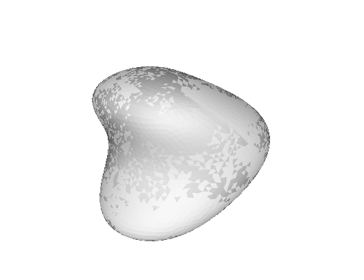
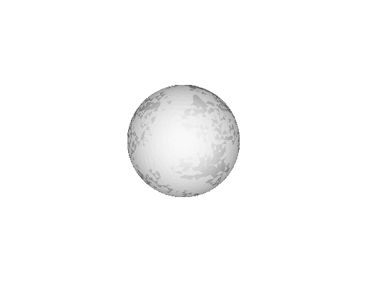
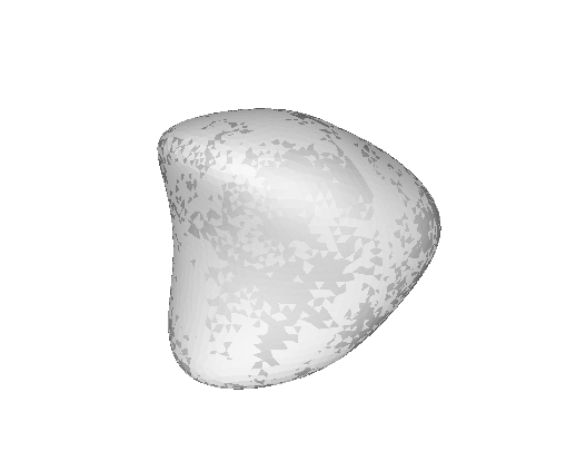
(a)                                     (b)                                (c)

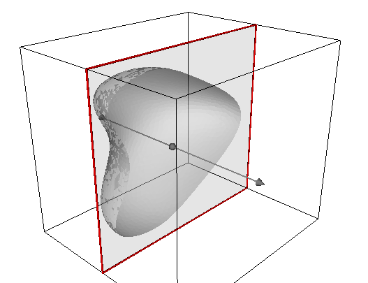
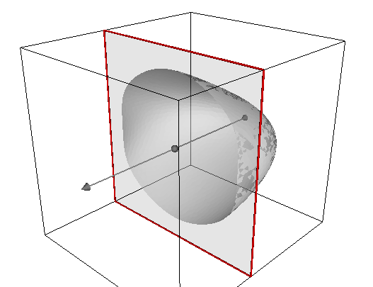
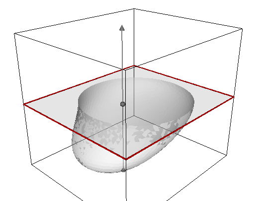
(d)                                     (e)                                (f)

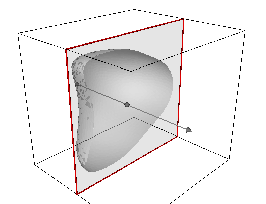
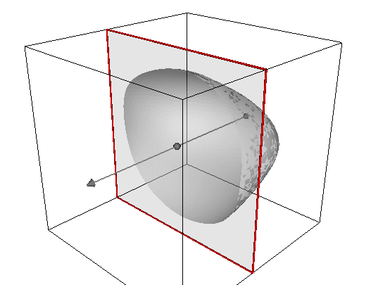
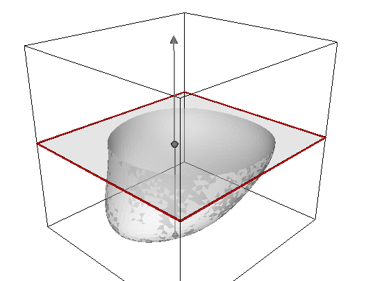
(g)                                     (h)                                (i)

Fig. 1: Example 1: A bean-shaped obstacle. (a) the exact surface; (b) the initial guess; (c) the reconstructed surface; (d)–(f) the corresponding cross section of the exact surface along plane $x_{1}=0,x_{2}=0,x_{3}=0$, respectively; (g)–(i) the corresponding cross section of the reconstructed surface along plane $x_{1}=0,x_{2}=0,x_{3}=0$, respectively.

Example 2. Consider a cushion-shaped obstacle:

$$\boldsymbol{r}(\theta,\varphi)=r(\theta,\varphi)(\sin(\theta)\cos(\varphi),\sin(\theta)\sin(\varphi),\cos(\theta))^{\top},~{}\theta\in[0,\pi],\,\varphi\in[0,2\pi],$$

where

$$r(\theta,\varphi)=\left(0.75+0.45(\cos(2\varphi)-1)(\cos(4\theta)-1)\right)^{1/2}.$$

Figure 2(a) shows the exact surface. This example is much more complex than the bean-shaped obstacle due to its multiple concave parts. Multiple incident directions are needed in order to obtain a good result. In this example, the obstacle is illuminated by the compressional wave from 6 directions, which are the unit vectors pointing to the origin from the face centers of the cube. The multiple frequencies are the same as the first example, i.e., the frequency ranges from $\omega_{\rm min}=1$ to $\omega_{\rm max}=5$ with $\omega_{i}=i+1,i=0,\dots,4$. For each fixed frequency and incident direction, repeat $L=50$ times with previous result as starting points. The step size for the decent method is $0.005/\omega_{i}$ and number of recovered coefficients is $6(\omega_{i}+2)^{2}$ for corresponding frequency. Figure 2(b) shows the initial guess ball with radius $R_{0}=0.5$; Figure 2(c) shows the final reconstructed surface; Figure 2(d)–(f) show the cross section of the exact surface along the plane $x_{1}=0,x_{2}=0,x_{3}=0$, respectively; while Figure 2(g)–(i) show the corresponding cross section for the reconstructed surface along the plane $x_{1}=0,x_{2}=0,x_{3}=0$, respectively. It is clear to note that the algorithm can also reconstruct effectively the more complex cushion-shaped obstacle.

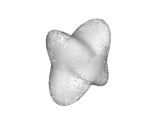
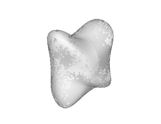
(a)                                     (b)                                (c)

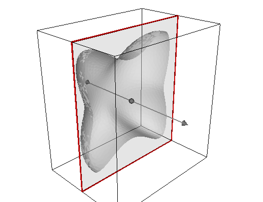
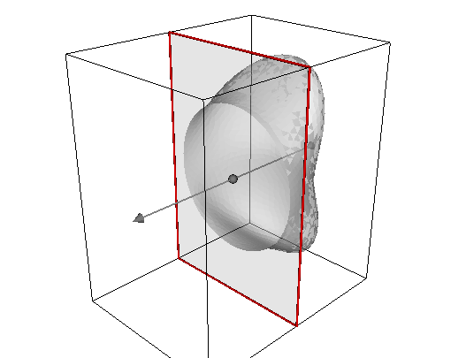
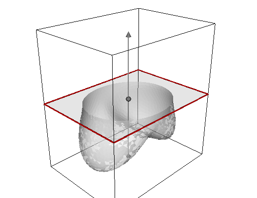
(d)                                     (e)                                (f)

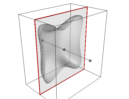
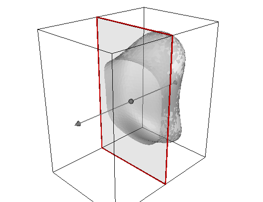
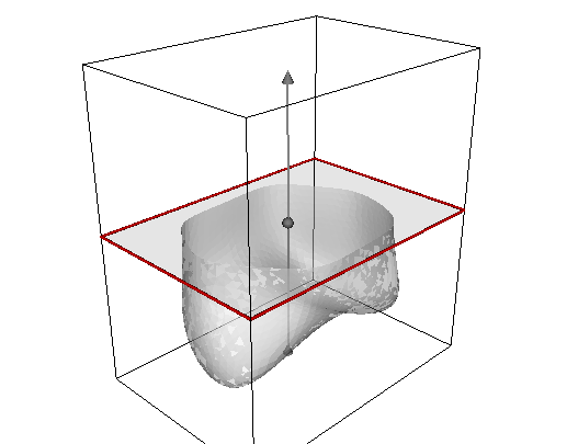
(g)                                     (h)                                (i)

Fig. 2: Example 2: A cushion-shaped obstacle. (a) the exact surface; (b) the initial guess; (c) the reconstructed surface; (d)–(f) the corresponding cross section of the exact surface along the plane $x_{1}=0,x_{2}=0,x_{3}=0$, respectively; (d)–(f) the corresponding cross section of the reconstructed surface along the plane $x_{1}=0,x_{2}=0,x_{3}=0$, respectively.

6 Conclusion

In this paper, we have studied the direct and inverse obstacle scattering problems for elastic waves in three dimensions. We develop an exact transparent boundary condition and show that the direct problem has a unique weak solution. We examine the domain derivative of the total displacement with respect to the surface of the obstacle. We propose a frequency continuation method for solving the inverse scattering problem. Numerical examples are presented to demonstrate the effectiveness of the proposed method. The results show that the method is stable and accurate to reconstruct surfaces with noise. Future work includes the surfaces of different boundary conditions and multiple obstacles where each obstacle’s surface has a parametric equation. We hope to be able to address these issues and report the progress elsewhere in the future.

Appendix A Spherical harmonics and functional spaces

The spherical coordinates $(r,\theta,\varphi)$ are related to the Cartesian coordinates $\boldsymbol{x}=(x_{1},x_{2},x_{3})$ by $x_{1}=r\sin\theta\cos\varphi,x_{2}=r\sin\theta\sin\varphi,x_{3}=r\cos\theta$. The local orthonormal basis is

$$\boldsymbol{e}_{r} =(\sin\theta\cos\varphi,\sin\theta\sin\varphi,\cos\theta)^{\top},$$

$$\boldsymbol{e}_{\theta} =(\cos\theta\cos\varphi,\cos\theta\sin\varphi,-\sin\theta)^{\top},$$

$$\boldsymbol{e}_{\varphi} =(-\sin\varphi,\cos\varphi,0)^{\top}.$$

Let $\{Y_{n}^{m}(\theta,\varphi):n=0,1,2,\dots,m=-n,\dots,n\}$ be the orthonormal sequence of spherical harmonics of order $n$ on the unit sphere. Define rescaled spherical harmonics

$$X_{n}^{m}(\theta,\varphi)=\frac{1}{R}Y_{n}^{m}(\theta,\varphi).$$

It can be shown that $\{X_{n}^{m}(\theta,\varphi):n=0,1,\dots,m=-n,\dots,n\}$ form a complete orthonormal system in $L^{2}(\Gamma_{R})$.

For a smooth scalar function $u(R,\theta,\varphi)$ defined on $\Gamma_{R}$, let

$$\nabla_{\Gamma_{R}}u=\partial_{\theta}u\,\boldsymbol{e}_{\theta}+(\sin\theta)^{-1}\partial_{\varphi}u\,\boldsymbol{e}_{\varphi}$$

be the tangential gradient on $\Gamma_{R}$. Define a sequence of vector spherical harmonics:

$$\boldsymbol{T}_{n}^{m}(\theta,\varphi) =\frac{1}{\sqrt{n(n+1)}}\nabla_{\Gamma_{R}}X_{n}^{m}(\theta,\varphi),$$

$$\boldsymbol{V}_{n}^{m}(\theta,\varphi) =\boldsymbol{T}_{n}^{m}(\theta,\varphi)\times\boldsymbol{e}_{r},\quad\boldsymbol{W}_{n}^{m}(\theta,\varphi)=X_{n}^{m}(\theta,\varphi)\boldsymbol{e}_{r},$$

where $n=0,1,\dots,m=-n,\dots,n$. Using the orthogonality of the vector spherical harmonics, we can also show that $\{(\boldsymbol{T}_{n}^{m},\boldsymbol{V}_{n}^{m},\boldsymbol{W}_{n}^{m}):n=0,1,2,\dots,m=-n,\dots,n\}$ form a complete orthonormal system in $\boldsymbol{L}^{2}(\Gamma_{R})=L^{2}(\Gamma_{R})^{3}$.

Let $\boldsymbol{L}^{2}(\Omega)=L^{2}(\Omega)^{3}$ be equipped with the inner product and norm:

$$(\boldsymbol{u},\boldsymbol{v})=\int_{\Omega}\boldsymbol{u}\cdot\bar{\boldsymbol{v}}\,{\rm d}\boldsymbol{x},\quad\|\boldsymbol{u}\|_{\boldsymbol{L}^{2}(\Omega)}=(\boldsymbol{u},\boldsymbol{u})^{1/2}.$$

Denote by $H^{1}(\Omega)$ the standard Sobolev space with the norm given by

$$\|u\|_{H^{1}(\Omega)}=\left(\int_{\Omega}|u(\boldsymbol{x})|^{2}+|\nabla u(\boldsymbol{x})|^{2}\,{\rm d}\boldsymbol{x}\right)^{1/2}.$$

Let $\boldsymbol{H}^{1}_{\partial D}(\Omega)=H^{1}_{\partial D}(\Omega)^{3}$, where $H^{1}_{\partial D}(\Omega):=\{u\in H^{1}(\Omega):u=0~{}\text{on}~{}\partial D\}$. Introduce the Sobolev space

$$\boldsymbol{H}({\rm curl},\Omega)=\{\boldsymbol{u}\in\boldsymbol{L}^{2}(\Omega),\nabla\times\boldsymbol{u}\in\boldsymbol{L}^{2}(\Omega)\},$$

which is equipped with the norm

$$\|\boldsymbol{u}\|_{\boldsymbol{H}({\rm curl},\Omega)}=\left(\|\boldsymbol{u}\|^{2}_{\boldsymbol{L}^{2}(\Omega)}+\|\nabla\times\boldsymbol{u}\|^{2}_{\boldsymbol{L}^{2}(\Omega)}\right)^{1/2}.$$

Denote by $H^{s}(\Gamma_{R})$ the trace functional space which is equipped with the norm

$$\|u\|_{H^{s}(\Gamma_{R})}=\left(\sum_{n=0}^{\infty}\sum_{m=-n}^{n}(1+n(n+1))^{s}|u_{n}^{m}|^{2}\right)^{1/2},$$

where

$$u(R,\theta,\varphi)=\sum_{n=0}^{\infty}\sum_{m=-n}^{n}u_{n}^{m}X_{n}^{m}(\theta,\varphi).$$

Let $\boldsymbol{H}^{s}(\Gamma_{R})=H^{s}(\Gamma_{R})^{3}$ which is equipped with the normal

$$\|\boldsymbol{u}\|_{\boldsymbol{H}^{s}(\Gamma_{R})}=\left(\sum_{n=0}^{\infty}\sum_{m=-n}^{n}(1+n(n+1))^{s}|\boldsymbol{u}_{n}^{m}|^{2}\right)^{1/2},$$

where $\boldsymbol{u}_{n}^{m}=(u_{1n}^{m},u_{2n}^{m},u_{3n}^{m})^{\top}$ and

$$\boldsymbol{u}(R,\theta,\varphi)=\sum_{n=0}^{\infty}\sum_{m=-n}^{n}u_{1n}^{m}\boldsymbol{T}_{n}^{m}(\theta,\varphi)+u_{2n}^{m}\boldsymbol{V}_{n}^{m}(\theta,\varphi)+u_{3n}^{m}\boldsymbol{W}_{n}^{m}(\theta,\varphi).$$

It can be verified that $\boldsymbol{H}^{-s}(\Gamma_{R})$ is the dual space of $\boldsymbol{H}^{s}(\Gamma_{R})$ with respect to the inner product

$$\langle\boldsymbol{u},\boldsymbol{v}\rangle_{\Gamma_{R}}=\int_{\Gamma_{R}}\boldsymbol{u}\cdot\bar{\boldsymbol{v}}\,{\rm d}\gamma=\sum_{n=0}^{\infty}\sum_{m=-n}^{n}u_{1n}^{m}\bar{v}_{1n}^{m}+u_{2n}^{m}\bar{v}_{2n}^{m}+u_{3n}^{m}\bar{v}_{3n}^{m},$$

where

$$\boldsymbol{v}(R,\theta,\varphi)=\sum_{n=0}^{\infty}\sum_{m=-n}^{n}v_{1n}^{m}\boldsymbol{T}_{n}^{m}(\theta,\varphi)+v_{2n}^{m}\boldsymbol{V}_{n}^{m}(\theta,\varphi)+v_{3n}^{m}\boldsymbol{W}_{n}^{m}(\theta,\varphi).$$

Introduce three tangential trace spaces:

$$\boldsymbol{H}_{\rm t}^{s}(\Gamma_{R}) =\{\boldsymbol{u}\in\boldsymbol{H}^{s}(\Gamma_{R}),~{}\boldsymbol{u}\cdot\boldsymbol{e}_{r}=0\},$$

$$\boldsymbol{H}^{-1/2}({\rm curl},\Gamma_{R}) =\{\boldsymbol{u}\in\boldsymbol{H}^{-1/2}_{\rm t}(\Gamma_{R}),~{}{\rm curl}_{\Gamma_{R}}\boldsymbol{u}\in H^{-1/2}(\Gamma_{R})\},$$

$$\boldsymbol{H}^{-1/2}({\rm div},\Gamma_{R}) =\{\boldsymbol{u}\in\boldsymbol{H}^{-1/2}_{\rm t}(\Gamma_{R}),~{}{\rm div}_{\Gamma_{R}}\boldsymbol{u}\in H^{-1/2}(\Gamma_{R})\}.$$

For any tangential field $\boldsymbol{u}\in\boldsymbol{H}^{s}_{\rm t}(\Gamma_{R})$, it can be represented in the series expansion

$$\boldsymbol{u}(R,\theta,\varphi)=\sum_{n=0}^{\infty}\sum_{m=-n}^{n}u_{1n}^{m}\boldsymbol{T}_{n}^{m}(\theta,\varphi)+u_{2n}^{m}\boldsymbol{V}_{n}^{m}(\theta,\varphi).$$

Using the series coefficients, the norm of the space $\boldsymbol{H}^{s}_{\rm t}(\Gamma_{R})$ can be characterized by

$$\|\boldsymbol{u}\|^{2}_{\boldsymbol{H}^{s}_{\rm t}(\Gamma_{R})}=\sum_{n=0}^{\infty}\sum_{m=-n}^{n}(1+n(n+1))^{s}\left(|u_{1n}^{m}|^{2}+|u_{2n}^{m}|^{2}\right);$$

the norm of the space $\boldsymbol{H}^{-1/2}({\rm curl},\Gamma_{R})$ can be characterized by

$$\|\boldsymbol{u}\|^{2}_{\boldsymbol{H}^{-1/2}({\rm curl},\Gamma_{R})}=\sum_{n=0}^{\infty}\sum_{m=-n}^{n}\frac{1}{\sqrt{1+n(n+1)}}|u_{1n}^{m}|^{2}+\sqrt{1+n(n+1)}|u_{2n}^{m}|^{2};$$

the norm of the space $\boldsymbol{H}^{-1/2}({\rm div},\Gamma_{R})$ can be characterized by

$$\|\boldsymbol{u}\|^{2}_{\boldsymbol{H}^{-1/2}({\rm div},\Gamma_{R})}=\sum_{n=0}^{\infty}\sum_{m=-n}^{n}\sqrt{1+n(n+1)}|u_{1n}^{m}|^{2}+\frac{1}{\sqrt{1+n(n+1)}}|u_{2n}^{m}|^{2}.$$

Given a vector field $\boldsymbol{u}$ on $\Gamma_{R}$, denote by $\boldsymbol{u}_{\Gamma_{R}}=-\boldsymbol{e}_{r}\times(\boldsymbol{e}_{r}\times\boldsymbol{u})$ the tangential component of $\boldsymbol{u}$ on $\Gamma_{R}$. Define the inner product in $\mathbb{C}^{3}$: $\langle\boldsymbol{u},\boldsymbol{v}\rangle=\boldsymbol{v}^{*}\boldsymbol{u},\forall\,\boldsymbol{u},\boldsymbol{v}\in\mathbb{C}^{3},$ where $\boldsymbol{v}^{*}$ is the conjugate transpose of $\boldsymbol{v}$.

Appendix B Transparent boundary conditions

Recall the Helmholtz decomposition (6):

$$\boldsymbol{v}=\nabla\phi+\nabla\times\boldsymbol{\psi},\quad\nabla\cdot\boldsymbol{\psi}=0,$$

where the scalar potential function $\phi$ satisfies (7) and (8):

(40) $$\begin{cases}\Delta\phi+\kappa^{2}_{\rm p}\phi=0&\quad\text{in}~{}\mathbb{R}^{3}\setminus\bar{D},\\ \partial_{r}\phi-{\rm i}\kappa_{\rm p}\phi=o(r^{-1})&\quad\text{as}~{}r\to\infty,\end{cases}$$

the vector potential function $\boldsymbol{\psi}$ satisfies (9) and (10):

(41) $$\begin{cases}\nabla\times(\nabla\times\boldsymbol{\psi})-\kappa^{2}_{\rm s}\boldsymbol{\psi}=0&\quad\text{in}~{}\mathbb{R}^{3}\setminus\bar{D},\\ (\nabla\times\boldsymbol{\psi})\times\hat{\boldsymbol{x}}-{\rm i}\kappa_{\rm s}\boldsymbol{\psi}=o(r^{-1})&\quad\text{as}~{}r\to\infty,\end{cases}$$

where $r=|\boldsymbol{x}|$ and $\hat{\boldsymbol{x}}=\boldsymbol{x}/r$.

In the exterior domain $\mathbb{R}^{3}\setminus\bar{B}_{R}$, the solution $\phi$ of (40) satisfies

(42) $$\phi(r,\theta,\varphi)=\sum_{n=0}^{\infty}\sum_{m=-n}^{n}\frac{h^{(1)}_{n}(\kappa_{\rm p}r)}{h^{(1)}_{n}(\kappa_{\rm p}R)}\phi_{n}^{m}X_{n}^{m}(\theta,\varphi),$$

where $h^{(1)}_{n}$ is the spherical Hankel function of the first kind with order $n$ and

$$\phi_{n}^{m}=\int_{\Gamma_{R}}\phi(R,\theta,\varphi)\bar{X}_{n}^{m}(\theta,\varphi){\rm d}\gamma.$$

We define the boundary operator $\mathscr{T}_{1}$ such that

(43) $$(\mathscr{T}_{1}\phi)(R,\theta,\varphi)=\frac{1}{R}\sum_{n=0}^{\infty}\sum_{m=-n}^{n}z_{n}(\kappa_{\rm p}R)\phi_{n}^{m}X_{n}^{m}(\theta,\varphi),$$

where $z_{n}(t)=th_{n}^{(1)^{\prime}}(t)/h_{n}^{(1)}(t)$ satisfies (cf. [31, Theorem 2.6.1])

(44) $$-(n+1)\leq{\rm Re}z_{n}(t)\leq-1,\quad 0<{\rm Im}z_{n}(t)\leq t.$$

Evaluating the derivative of (42) with respect to $r$ at $r=R$ and using (43), we get the transparent boundary condition for the scalar potential function $\phi$:

(45) $$\partial_{r}\phi=\mathscr{T}_{1}\phi\quad\text{on}~{}\Gamma_{R}.$$

The following result can be easily shown from (43)–(44).

Lemma 10.

The operator $\mathscr{T}_{1}$ is bounded from $H^{1/2}(\Gamma_{R})$ to $H^{-1/2}(\Gamma_{R})$. Moreover, it satisfies

$${\rm Re}\langle\mathscr{T}_{1}u,u\rangle_{\Gamma_{R}}\leq 0,\quad{\rm Im}\langle\mathscr{T}_{1}u,u\rangle_{\Gamma_{R}}\geq 0,\quad\forall u\in H^{1/2}(\Gamma_{R}).$$

If ${\rm Re}\langle\mathscr{T}_{1}u,u\rangle_{\Gamma_{R}}=0$ or ${\rm Im}\langle\mathscr{T}_{1}u,u\rangle_{\Gamma_{R}}=0$, then $u=0$ on $\Gamma_{R}$.

Define an auxiliary function $\boldsymbol{\varphi}=({\rm i}\kappa_{\rm s})^{-1}\nabla\times\boldsymbol{\psi}$. We have from (41) that

(46) $$\nabla\times\boldsymbol{\psi}-{\rm i}\kappa_{\rm s}\boldsymbol{\varphi}=0,\quad\nabla\times\boldsymbol{\varphi}+{\rm i}\kappa_{\rm s}\boldsymbol{\psi}=0,$$

which are Maxwell’s equations. Hence $\boldsymbol{\phi}$ and $\boldsymbol{\psi}$ plays the role of the electric field and the magnetic field, respectively.

Introduce the vector wave functions

(47) $$\begin{cases}\boldsymbol{M}_{n}^{m}(r,\theta,\varphi)=\nabla\times(\boldsymbol{x}h_{n}^{(1)}(\kappa_{\rm s}r)X_{n}^{m}(\theta,\varphi)),\\ \boldsymbol{N}_{n}^{m}(r,\theta,\varphi)=({\rm i}\kappa_{\rm s})^{-1}\nabla\times\boldsymbol{M}_{n}^{m}(r,\theta,\varphi),\end{cases}$$

which are the radiation solutions of (46) in $\mathbb{R}^{3}\setminus\{0\}$ (cf. [30, Theorem 9.16]):

$$\nabla\times\boldsymbol{M}_{n}^{m}(r,\theta,\varphi)-{\rm i}\kappa_{\rm s}\boldsymbol{N}_{n}^{m}(r,\theta,\varphi)=0,\quad\nabla\times\boldsymbol{N}_{n}^{m}(r,\theta,\varphi)+{\rm i}\kappa_{\rm s}\boldsymbol{M}_{n}^{m}(r,\theta,\varphi)=0.$$

Moreover, it can be verified from (47) that they satisfy

(48) $$\boldsymbol{M}_{n}^{m}=h_{n}^{{(1)}}(\kappa_{\rm s}r)\nabla_{\Gamma_{R}}X_{n}^{m}\times\boldsymbol{e}_{r}$$

and

(49) $$\boldsymbol{N}_{n}^{m}=\frac{\sqrt{n(n+1)}}{{\rm i}\kappa_{\rm s}r}(h_{n}^{(1)}(\kappa_{\rm s}r)+\kappa_{\rm s}rh_{n}^{(1)^{\prime}}(\kappa_{\rm s}r))\boldsymbol{T}_{n}^{m}+\frac{n(n+1)}{{\rm i}\kappa_{\rm s}r}h_{n}^{(1)}(\kappa_{\rm s}r)\boldsymbol{W}_{n}^{m}.$$

In the domain $\mathbb{R}^{3}\setminus\bar{B}_{R}$, the solution of $\boldsymbol{\psi}$ in (46) can be written in the series

(50) $$\boldsymbol{\psi}=\sum_{n=0}^{\infty}\sum_{m=-n}^{n}\alpha_{n}^{m}\boldsymbol{N}_{n}^{m}+\beta_{n}^{m}\boldsymbol{M}_{n}^{m},$$

which is uniformly convergent on any compact subsets in $\mathbb{R}^{3}\setminus\bar{B}_{R}$. Correspondingly, the solution of $\boldsymbol{\varphi}$ in (46) is given by

(51) $$\boldsymbol{\varphi}=({\rm i}\kappa_{\rm s})^{-1}\nabla\times\boldsymbol{\psi}=\sum_{n=0}^{\infty}\sum_{m=-n}^{n}\beta_{n}^{m}\boldsymbol{N}_{n}^{m}-\alpha_{n}^{m}\boldsymbol{M}_{n}^{m}.$$

It follows from (48)–(49) that

$$-\boldsymbol{e}_{r}\times(\boldsymbol{e}_{r}\times\boldsymbol{M}_{n}^{m}) =-\sqrt{n(n+1)}h_{n}^{(1)}(\kappa_{\rm s}r)\boldsymbol{V}_{n}^{m},$$

$$-\boldsymbol{e}_{r}\times(\boldsymbol{e}_{r}\times\boldsymbol{N}_{n}^{m}) =\frac{\sqrt{n(n+1)}}{{\rm i}\kappa_{\rm s}r}(h_{n}^{(1)}(\kappa_{\rm s}r)+\kappa_{\rm s}rh_{n}^{(1)^{\prime}}(\kappa_{\rm s}r))\boldsymbol{T}_{n}^{m}$$

and

$$\boldsymbol{e}_{r}\times\boldsymbol{M}_{n}^{m} =\sqrt{n(n+1)}h_{n}^{(1)}(\kappa_{\rm s}r)\boldsymbol{T}_{n}^{m},$$

$$\boldsymbol{e}_{r}\times\boldsymbol{N}_{n}^{m} =\frac{\sqrt{n(n+1)}}{{\rm i}\kappa_{\rm s}r}(h_{n}^{(1)}(\kappa_{\rm s}r)+\kappa_{\rm s}rh_{n}^{(1)^{\prime}}(\kappa_{\rm s}r))\boldsymbol{V}_{n}^{m}.$$

Therefore, by (50), the tangential component of $\boldsymbol{\psi}$ on $\Gamma_{R}$ is

$$\boldsymbol{\psi}_{\Gamma_{R}}=\sum_{n=0}^{\infty}\sum_{m=-n}^{n}\frac{\sqrt{n(n+1)}}{{\rm i}\kappa_{\rm s}R}(h_{n}^{(1)}(\kappa_{\rm s}R)+\kappa_{\rm s}Rh_{n}^{(1)^{\prime}}(\kappa_{\rm s}R))\alpha_{n}^{m}\boldsymbol{T}_{n}^{m}+\sqrt{n(n+1)}h_{n}^{(1)}(\kappa_{\rm s}R)\beta_{n}^{m}\boldsymbol{V}_{n}^{m}.$$

Similarly, by (51), the tangential trace of $\boldsymbol{\varphi}$ on $\Gamma_{R}$ is

$$\boldsymbol{\varphi}\times\boldsymbol{e}_{r} =\sum_{n=0}^{\infty}\sum_{m=-n}^{n}\sqrt{n(n+1)}h_{n}^{(1)}(\kappa_{\rm s}R)\alpha_{n}^{m}\boldsymbol{T}_{n}^{m}$$

$$\qquad-\frac{\sqrt{n(n+1)}}{{\rm i}\kappa_{\rm s}R}(h_{n}^{(1)}(\kappa_{\rm s}R)+\kappa_{\rm s}Rh_{n}^{(1)^{\prime}}(\kappa_{\rm s}R))\beta_{n}^{m}\boldsymbol{V}_{n}^{m}.$$

Given any tangential component of the electric field on $\Gamma_{R}$ with the expression

$$\boldsymbol{u}=\sum_{n=0}^{\infty}\sum_{m=-n}^{n}u_{1n}^{m}\boldsymbol{T}_{n}^{m}+u_{2n}^{m}\boldsymbol{V}_{n}^{m},$$

we define

(52) $$\mathscr{T}_{2}\boldsymbol{u}=\sum_{n=0}^{\infty}\sum_{m=-n}^{n}\frac{{\rm i}\kappa_{\rm s}R}{1+z_{n}(\kappa_{\rm s}R)}u_{1n}^{m}\boldsymbol{T}_{n}^{m}+\frac{1+z_{n}(\kappa_{\rm s}R)}{{\rm i}\kappa_{\rm s}R}u_{2n}^{m}\boldsymbol{V}_{n}^{m}.$$

Using (52), we obtain the transparent boundary condition for $\boldsymbol{\psi}$:

(53) $$(\nabla\times\boldsymbol{\psi})\times\boldsymbol{e}_{r}={\rm i}\kappa_{\rm s}\mathscr{T}_{2}\boldsymbol{\psi}_{\Gamma_{R}}\quad\text{on}~{}\Gamma_{R}.$$

The following result can also be easily shown from (44) and (52)

Lemma 11.

The operator $\mathscr{T}_{2}$ is bounded from $\boldsymbol{H}^{1/2}({\rm curl},\Gamma_{R})$ to $\boldsymbol{H}^{-1/2}({\rm div},\Gamma_{R})$. Moreover, it satisfies

$${\rm Re}\langle\mathscr{T}_{2}\boldsymbol{u},\boldsymbol{u}\rangle_{\Gamma_{R}}\geq 0,\quad\forall\boldsymbol{u}\in\boldsymbol{H}^{1/2}({\rm curl},\Gamma_{R}).$$

If ${\rm Re}\langle\mathscr{T}_{2}\boldsymbol{u},\boldsymbol{u}\rangle_{\Gamma_{R}}=0$, then $\boldsymbol{u}=0$ on $\Gamma_{R}$.

Appendix C Fourier coefficients

We derive the mutual representations of the Fourier coefficients between $\boldsymbol{v}$ and $(\phi,\boldsymbol{\psi})$. First we have from (42) that

(54) $$\phi(r,\theta,\varphi)=\sum_{n=0}^{\infty}\sum_{m=-n}^{n}\frac{h^{(1)}_{n}(\kappa_{\rm p}r)}{h^{(1)}_{n}(\kappa_{\rm p}R)}\phi_{n}^{m}X_{n}^{m}(\theta,\varphi).$$

Substituting (48)–(49) into (50) yields

$$\boldsymbol{\psi}(r,\theta,\varphi) =\sum_{n=0}^{\infty}\sum_{m=-n}^{n}\frac{\sqrt{n(n+1)}}{{\rm i}\kappa_{\rm s}r}(h_{n}^{(1)}(\kappa_{\rm s}r)+\kappa_{\rm s}rh_{n}^{(1)^{\prime}}(\kappa_{\rm s}r))\alpha_{n}^{m}\boldsymbol{T}_{n}^{m}$$

(55) $$\qquad+\sqrt{n(n+1)}h_{n}^{(1)}(\kappa_{\rm s}r)\beta_{n}^{m}\boldsymbol{V}_{n}^{m}+\frac{n(n+1)}{{\rm i}\kappa_{\rm s}r}h_{n}^{(1)}(\kappa_{\rm s}r)\alpha_{n}^{m}\boldsymbol{W}_{n}^{m}.$$

Given $\boldsymbol{\psi}$ on $\Gamma_{R}$, it has the Fourier expansion:

(56) $$\boldsymbol{\psi}(R,\theta,\varphi)=\sum_{n=0}^{\infty}\sum_{m=-n}^{n}\psi_{1n}^{m}\boldsymbol{T}_{n}^{m}(\theta,\varphi)+\psi_{2n}^{m}\boldsymbol{V}_{n}^{m}(\theta,\varphi)+\psi_{3n}^{m}\boldsymbol{W}_{n}^{m}(\theta,\varphi).$$

Evaluating (C) at $r=R$ and then comparing it with (56), we get

(57) $$\alpha_{n}^{m}=\frac{{\rm i}\kappa_{\rm s}R}{n(n+1)h_{n}^{(1)}(\kappa_{\rm s}R)}\psi_{3n}^{m},\quad\beta_{n}^{m}=\frac{1}{\sqrt{n(n+1)}h_{n}^{(1)}(\kappa_{\rm s}R)}\psi_{2n}^{m}.$$

Plugging (57) back into (C) gives

$$\boldsymbol{\psi}(r,\theta,\varphi) =\sum_{n=0}^{\infty}\sum_{m=-n}^{n}\left(\frac{R}{r}\right)\left(\frac{h_{n}^{(1)}(\kappa_{\rm s}r)+\kappa_{\rm s}rh_{n}^{(1)^{\prime}}(\kappa_{\rm s}r)}{\sqrt{n(n+1)}h_{n}^{(1)}(\kappa_{\rm s}R)}\right)\psi_{3n}^{m}\boldsymbol{T}_{n}^{m}$$

(58) $$\qquad+\left(\frac{h_{n}^{(1)}(\kappa_{\rm s}r)}{h_{n}^{(1)}(\kappa_{\rm s}R)}\right)\psi_{2n}^{m}\boldsymbol{V}_{n}^{m}+\left(\frac{R}{r}\right)\left(\frac{h_{n}^{(1)}(\kappa_{\rm s}r)}{h_{n}^{(1)}(\kappa_{\rm s}R)}\right)\psi_{3n}^{m}\boldsymbol{W}_{n}^{m}.$$

Noting $\nabla\phi=\partial_{r}\phi\,\boldsymbol{e}_{r}+\frac{1}{r}\nabla_{\Gamma_{R}}\phi$, we have from (54) and (C) that

$$\nabla\phi =\sum_{n=0}^{\infty}\sum_{m=-n}^{n}\left(\frac{\kappa_{\rm p}h^{(1)^{\prime}}_{n}(\kappa_{\rm p}r)}{h^{(1)}_{n}(\kappa_{\rm p}R)}\right)\phi_{n}^{m}X_{n}^{m}\boldsymbol{e}_{r}+\left(\frac{h^{(1)}_{n}(\kappa_{\rm p}r)}{rh^{(1)}_{n}(\kappa_{\rm p}R)}\right)\phi_{n}^{m}\nabla_{\Gamma_{R}}X_{n}^{m}$$

$$=\sum_{n=0}^{\infty}\sum_{m=-n}^{n}\left(\frac{\kappa_{\rm p}h^{(1)^{\prime}}_{n}(\kappa_{\rm p}r)}{h^{(1)}_{n}(\kappa_{\rm p}R)}\right)\phi_{n}^{m}\boldsymbol{W}_{n}^{m}+\left(\frac{\sqrt{n(n+1)}h^{(1)}_{n}(\kappa_{\rm p}r)}{rh^{(1)}_{n}(\kappa_{\rm p}R)}\right)\phi_{n}^{m}\boldsymbol{T}_{n}^{m}.$$

and

$$\nabla\times\boldsymbol{\psi}=\sum_{n=0}^{\infty}\sum_{m=-n}^{n}\boldsymbol{I}_{1n}^{m}+\boldsymbol{I}_{2n}^{m}+\boldsymbol{I}_{3n}^{m},$$

where

$$\boldsymbol{I}_{1n}^{m} =\nabla\times\left[\left(\frac{R}{r}\right)\left(\frac{h_{n}^{(1)}(\kappa_{\rm s}r)+\kappa_{\rm s}rh_{n}^{(1)^{\prime}}(\kappa_{\rm s}r)}{\sqrt{n(n+1)}h_{n}^{(1)}(\kappa_{\rm s}R)}\right)\psi_{3n}^{m}\boldsymbol{T}_{n}^{m}\right]$$

$$=\frac{Rh_{n}^{(1)}(\kappa_{\rm s}r)}{\sqrt{n(n+1)}h_{n}^{(1)}(\kappa_{\rm s}R)}\left(\kappa^{2}_{\rm s}-\frac{n(n+1)}{r^{2}}\right)\psi_{3n}^{m}\boldsymbol{V}_{n}^{m},$$

$$\boldsymbol{I}_{2n}^{m} =\nabla\times\left[\left(\frac{h_{n}^{(1)}(\kappa_{\rm s}r)}{h_{n}^{(1)}(\kappa_{\rm s}R)}\right)\psi_{2n}^{m}\boldsymbol{V}_{n}^{m}\right]$$

$$=\left(\frac{h_{n}^{(1)}(\kappa_{\rm s}r)+\kappa_{\rm s}rh_{n}^{(1)^{\prime}}(\kappa_{\rm s}r)}{rh_{n}^{(1)}(\kappa_{\rm s}R)}\right)\psi_{2n}^{m}\boldsymbol{T}_{n}^{m}+\frac{\sqrt{n(n+1)}h_{n}^{(1)}(\kappa_{\rm s}r)}{rh_{n}^{(1)}(\kappa_{\rm s}R)}\psi_{2n}^{m}\boldsymbol{W}_{n}^{m},$$

$$\boldsymbol{I}_{3n}^{m} =\nabla\times\left[\left(\frac{R}{r}\right)\left(\frac{h_{n}^{(1)}(\kappa_{\rm s}r)}{h_{n}^{(1)}(\kappa_{\rm s}R)}\right)\psi_{3n}^{m}\boldsymbol{W}_{n}^{m}\right]=\frac{R\sqrt{n(n+1)}h_{n}^{(1)}(\kappa_{\rm s}r)}{r^{2}h_{n}^{(1)}(\kappa_{\rm s}R)}\psi_{3n}^{m}\boldsymbol{V}_{n}^{m}.$$

Combining the above equations and noting $\boldsymbol{v}=\nabla\phi+\nabla\times\boldsymbol{\psi}$, we obtain

$$\boldsymbol{v}(r,\theta,\varphi)=\sum_{n=0}^{\infty}\sum_{m=-n}^{n}\left(\frac{\sqrt{n(n+1)}h^{(1)}_{n}(\kappa_{\rm p}r)}{rh^{(1)}_{n}(\kappa_{\rm p}R)}\phi_{n}^{m}+\frac{(h_{n}^{(1)}(\kappa_{\rm s}r)+\kappa_{\rm s}rh_{n}^{(1)^{\prime}}(\kappa_{\rm s}r))}{rh_{n}^{(1)}(\kappa_{\rm s}R)}\psi_{2n}^{m}\right)\boldsymbol{T}_{n}^{m}$$

(59) $$\qquad+\frac{\kappa^{2}_{\rm s}Rh_{n}^{(1)}(\kappa_{\rm s}r)}{\sqrt{n(n+1)}h_{n}^{(1)}(\kappa_{\rm s}R)}\psi_{3n}^{m}\boldsymbol{V}_{n}^{m}+\left(\frac{\kappa_{\rm p}h^{(1)^{\prime}}_{n}(\kappa_{\rm p}r)}{h^{(1)}_{n}(\kappa_{\rm p}R)}\phi_{n}^{m}+\frac{\sqrt{n(n+1)}h_{n}^{(1)}(\kappa_{\rm s}r)}{rh_{n}^{(1)}(\kappa_{\rm s}R)}\psi_{2n}^{m}\right)\boldsymbol{W}_{n}^{m},$$

which gives

$$\boldsymbol{v}(R,\theta,\varphi)= \sum_{n=0}^{\infty}\sum_{m=-n}^{n}\frac{1}{R}\left(\sqrt{n(n+1)}\phi_{n}^{m}+(1+z_{n}(\kappa_{\rm s}R))\psi_{2n}^{m}\right)\boldsymbol{T}_{n}^{m}$$

(60) $$+\frac{\kappa^{2}_{\rm s}R}{\sqrt{n(n+1)}}\psi_{3n}^{m}\boldsymbol{V}_{n}^{m}+\frac{1}{R}\left(z_{n}(\kappa_{\rm p}R)\phi_{n}^{m}+\sqrt{n(n+1)}\psi_{2n}^{m}\right)\boldsymbol{W}_{n}^{m}.$$

On the other hand, $\boldsymbol{v}$ has the Fourier expansion:

(61) $$\boldsymbol{v}(R,\theta,\varphi)=\sum_{n=0}^{\infty}\sum_{m=-n}^{n}v_{1n}^{m}\boldsymbol{T}_{n}^{m}+v_{2n}^{m}\boldsymbol{V}_{n}^{m}+v_{3n}^{m}\boldsymbol{W}_{n}^{m}.$$

Comparing (C) with (61), we obtain

(62) $$\begin{cases}v_{1n}^{m}=\dfrac{\sqrt{n(n+1)}}{R}\phi_{n}^{m}+\dfrac{(1+z_{n}(\kappa_{\rm s}R))}{R}\psi_{2n}^{m},\\[5.0pt] v_{2n}^{m}=\dfrac{\kappa^{2}_{\rm s}R}{\sqrt{n(n+1)}}\psi_{3n}^{m},\\[5.0pt] v_{3n}^{m}=\dfrac{z_{n}(\kappa_{\rm p}R)}{R}\phi_{n}^{m}+\dfrac{\sqrt{n(n+1)}}{R}\psi_{2n}^{m},\end{cases}$$

and

(63) $$\begin{cases}\phi_{n}^{m}=\dfrac{R(1+z_{n}(\kappa_{\rm s}R))}{\Lambda_{n}}v_{3n}^{m}-\dfrac{R\sqrt{n(n+1)}}{\Lambda_{n}}v_{1n}^{m},\\[5.0pt] \psi_{2n}^{m}=\dfrac{Rz_{n}(\kappa_{\rm p}R)}{\Lambda_{n}}v_{1n}^{m}-\dfrac{R\sqrt{n(n+1)}}{\Lambda_{n}}v_{3n}^{m},\\[5.0pt] \psi_{3n}^{m}=\dfrac{\sqrt{n(n+1)}}{\kappa_{\rm s}^{2}R}v_{2n}^{m},\end{cases}$$

where

$$\Lambda_{n}=z_{n}(\kappa_{\rm p}R)(1+z_{n}(\kappa_{\rm s}R))-n(n+1).$$

Noting (44), we have from a simple calculation that

$${\rm Im}\Lambda_{n}={\rm Re}z_{n}(\kappa_{\rm p}R){\rm Im}z_{n}(\kappa_{\rm s}R)+(1+{\rm Re}z_{n}(\kappa_{\rm s}R)){\rm Im}z_{n}(\kappa_{\rm p}R)<0,$$

which implies that $\Lambda_{n}\neq 0$ for $n=0,1,\dots.$

References

- [1] C. Alves and H. Ammari, Boundary integral formula for the reconstruction of imperfections of small diameter in an elastic medium, SIAM J. Appl. Math. 62 (2001), 94–106.
- [2] H. Ammari, E. Bretin, J. Garnier, H. Kang, H. Lee, and A. Wahab, Mathematical Methods in Elasticity Imaging, Princeton University Press, New Jersey, 2015.
- [3] G. Bao, G. Hu, J. Sun, and T. Yin, Direct and inverse elastic scattering from anisotropic media, preprint.
- [4] G. Bao, P. Li, J. Lin, and F. Triki, Inverse scattering problems with multi-frequencies, Inverse Problems, 31 (2015), 093001.
- [5] M. Bonnet and A. Constantinescu, Inverse problems in elasticity Inverse Problems, 21 (2005), 1–50.
- [6] A. Charalambopoulos, D. Gintides, and K. Kiriaki, On the uniqueness of the inverse elastic scattering problem for periodic structures, Inverse Problems, 17 (2001), 1923–1935.
- [7] D. Colton and R. Kress, Integral Equation Methods in Scattering Theory, Wiley, New York, 1983.
- [8] D. Colton and R. Kress, Inverse Acoustic and Electromagnetic Scattering Theory, Springer-Verlag, Berlin, 1998.
- [9] J. Elschner and M. Yamamoto, Uniqueness in inverse elastic scattering with finitely many incident waves, Inverse Problems 26 (2010), 045005.
- [10] H. Haddar and R. Kress, On the Fréchet derivative for obstacle scattering with an impedance boundary condition, SIAM J. Appl. Math., 65 (2004), 94–208.
- [11] P. Hähner and G. C. Hsiao, Uniqueness theorems in inverse obstacle scattering of elastic waves, Inverse Problems, 9 (1993), 525–534.
- [12] F. Hecht, New development in FreeFem++, J. Numer. Math., 20 (2012), 251–265.
- [13] G. Hu, A. Kirsch, and M. Sini, Some inverse problems arising from elastic scattering by rigid obstacles, Inverse Problems, 29 (2013), 015009
- [14] G. Hu, J. Li, H. Liu, and H. Sun, Inverse elastic scattering for multiscale rigid bodies with a single far-field pattern, SIAM J. Imaging Sci., 7 (2014), 1799–1825.
- [15] G. Hu, Y. Lu, and B. Zhang, The factorization method for inverse elastic scattering from periodic structures, Inverse Problems, 29 (2013), 115005.
- [16] A. Kirsch, The domain derivative and two applications in inverse scattering theory, Inverse Problems, 9 (1993), 81–96.
- [17] R. Kress, Inverse elastic scattering from a crack, Inverse Problems, 12 (1996), 667–684.
- [18] M. Kar and M. Sini, On the inverse elastic scattering by interfaces using one type of scattered waves, J. Elast., 118 (2015), 15–38.
- [19] F. Le Louër, A domain derivative-based method for solving elastodynamic inverse obstacle scattering problems, Inverse Problems, 31 (2015), 115006.
- [20] F. Le Louër, On the Fréchet derivative in elastic obstacle scattering, SIAM J. Appl. Math., 72 (2012), pp. 1493–1507.
- [21] L.D. Landau and E.M. Lifshitz, Theory of Elasticity, Oxford: Pergamon Press, 1986
- [22] P. Li and Y. Wang, Near-field imaging of small perturbed obstacles for elastic waves, Inverse Problems, 31 (2015), 085010.
- [23] P. Li, Y. Wang, Z. Wang, and Y. Zhao, Inverse obstacle scattering for elastic waves, Inverse Problems, 32 (2016), 115018.
- [24] P. Li, Y. Wang, and Y. Zhao, Inverse elastic surface scattering with near-field data, Inverse Problems, 31 (2015), 035009.
- [25] P. Li, Y. Wang, and Y. Zhao, Near-field imaging of biperiodic surfaces for elastic waves, J. Comput. Phys., 324 (2016), 1–23.
- [26] P. Li, Y. Wang, and Y. Zhao, Convergence analysis in near-field imaging for elastic waves, Applicable Analysis, 95 (2016), 2339–2360.
- [27] G. Nakamura and K. Tanuma, A nonuniqueness theorem for an inverse boundary value problem arising in elasticity, SIAM J. Appl. Math., 56 (1996), 602–610.
- [28] G. Nakamura and G. Uhlmann, Inverse problems at the boundary of elastic medium, SIAM J. Math. Anal., 26 (1995), 263–279.
- [29] G. Nakamura and G. Uhlmann, Global uniqueness for an inverse boundary problem arising in elasticity, Invent. Math., 118 (1994), 457–474.
- [30] P. Monk, Finite Element Methods for Maxwell’s Equations, Oxford University Press, New York, 2003.
- [31] J.-C. Nédélec, Acoustic and Electromagnetic Equations Integral Representations for Harmonic Problems, Springer, 2000.
- [32] R. Potthast, Domain derivatives in electromagnetic scattering, Math. Meth. Appl. Sci., 19 (1996), pp. 1157–1175.
- [33] J. Tittelfitz, An inverse source problem for the elastic wave in the lower-half space, SIAM J. Appl. Math., 75 (2015), 1599–1619.
- [34] G. N. Watson, A Treatise on the Theory of Bessel Functions, Cambridge University Press, Cambridge, UK, 1922.