Thermal properties of a string bit model at large $N$

Abstract

We study the finite temperature properties of a recently introduced string bit model designed to capture some features of the emergent string in the tensionless limit. The model consists of a pair of bosonic and fermionic bit operators transforming in the adjoint representation of the color group $SU(N)$. Color confinement is not achieved as a dynamical effect, but instead is enforced by an explicit singlet projection. At large $N$ and finite temperature, the model has a non trivial thermodynamics. In particular, there is a Hagedorn type transition at a finite temperature $T=T_{\rm H}$ where the string degrees of freedom are liberated and the free energy gets a large contribution $\sim N^{2}$ that plays the role of an order parameter. For $T>T_{\rm H}$, the low temperature phase becomes unstable. In the new phase, the thermodynamically favoured configurations are characterized by a non-trivial gapped density of the $SU(N)$ angles associated with the singlet projection. We present an accurate algorithm for the determination of the density profile at $N=\infty$. In particular, we determine the gap endpoint at generic temperature and analytical expansions valid near the Hagedorn transition as well as at high temperature. The leading order corrections are characterized by non-trivial exponents that are determined analytically and compared with explicit numerical calculations.

1 Introduction and summary of results

Thorn’s string bits models have been originally proposed as a description of superstrings where stability and causality are manifest Giles:1977mpa ; Thorn:1991fv ; Bergman:1995wh ; Sun:2014dga ; Thorn:2014hia . In the framework of ’t Hooft $1/N$ expansion and light-cone parametrization of the string, one considers the continuum limit of very long chains composed of elementary string bits transforming in the adjoint of the color gauge group $SU(N)$. When the number of bits $M$ gets large, the bit chains behave approximately like continuous strings with recovered Lorentz invariance.  The finite temperature thermodynamics of such string bit models is quite rich in the ’t Hooft large $N$ limit. Stringy low energy states turn out to be color singlets separated from non-singlets by an infinite gap in units of the characteristic singlet energy $\sim 1/M$ Sun:2014dga ; Thorn:2014hia . This means that color confinement emerges as a consequence of the dynamics. Besides, the singlet subspace exhibits a Hagedorn transition Hagedorn:1965st at infinite $N$ tHooft:1973alw ; Thorn:1980iv signalled by a divergence of the partition function for temperatures above a certain finite temperature $T>T_{\rm H}$. As usual, this behaviour is generically associated with a density of states growing exponentially with energy as in the original dual resonance models Fubini:1969qb or modern string theory Atick:1988si . When string perturbation theory is identified with the ’t Hooft $1/N$ expansion of string bit dynamics, the $N=\infty$ Hagedorn transition is consistent the interpretation of $T_{\rm H}$ in the free string as an artifact of the zero coupling limit Atick:1988si with a possible phase transition near $T_{\rm H}$ to a phase dominated by the fundamental degrees of freedom of the emergent string theory.

Recently and remarkably, the Hagedorn transition of string bit models has been further clarified Thorn:2015bia , and discovered also in simpler reduced systems where the singlet restriction is imposed from the beginning as a kinematical constraint and not as a dynamical feature Raha:2017jgv ; Curtright:2017pfq . The starting point is the thermal partition function

$$Z=\text{tr}\,e^{-\beta\,(H+\mu\,M)},$$ (1)

where $\beta$ is the inverse temperature, $H$ the string bit model Hamiltonian, and $M$ is the bit number operator associated with the chemical potential $\mu$. The partition function (1) is quite natural and has a simple origin from the light-cone description of the emergent string where $H=P^{-}/\sqrt{2}$, $\mu\,M=P^{+}/\sqrt{2}$, and thus $H+\mu\,M=P^{0}=(P^{+}+P^{-})/\sqrt{2}$ Goddard:1973qh . The reduced model considered in Raha:2017jgv ; Curtright:2017pfq is the projection of (1) on the subspace of singlets states with $H=0$, i.e. for the associated tensionless string, and is described by the simpler partition function

$$Z_{0}=\text{tr}_{\rm singlets}\,x^{M},\qquad x=e^{-\beta\,\mu}.$$ (2)

Here, we shall focus on the simple model considered in Raha:2017jgv which consists of one pair of bosonic and fermionic string bits operators $a$ and $b$, both transforming in the adjoint of $SU(N)$. Extensions to models with more bit species and discussion of $1/N$ corrections have been addressed in Curtright:2017pfq . The bit number operator is $M=\text{tr}(\overline{a}\,a+\overline{b}\,b)$, where trace is in color space, and the projected partition function (2) can be computed by group averaging according to the analysis of Raha:2017jgv ; Curtright:2017pfq

$$Z_{0} =\frac{1-x}{1+x}\,\int dU(\bm{\vartheta})\,\text{tr}(x^{M}\,e^{i\,G_{k}\vartheta_{k}})=\frac{1-x}{1+x}\,\int dU(\bm{\vartheta})\,\prod_{1\leq k<\ell\leq N}\frac{1+x\,e^{i\,(\vartheta_{k}-\vartheta_{\ell})}}{1-x\,e^{i\,(\vartheta_{k}-\vartheta_{\ell})}}$$

$$=\left(\frac{1+x}{1-x}\right)^{N-1}\,\int dU(\bm{\vartheta})\,\prod_{1\leq k<\ell\leq N}\frac{1+x^{2}+2\,x\,\cos(\vartheta_{k}-\vartheta_{\ell})}{1+x^{2}-2\,x\,\cos(\vartheta_{k}-\vartheta_{\ell})},$$ (3)

where $G_{k}$ span the Cartan subalgebra of $U(N)$. The group integration in (1) is with respect to the normalized Haar measure

$$dU(\bm{\vartheta})=\frac{1}{N!\,(2\pi)^{N}}\,\int_{-\pi}^{\pi}d^{N}\bm{\vartheta}\,\prod_{1\leq k<\ell\leq N}\,4\,\sin^{2}\left(\frac{\vartheta_{k}-\vartheta_{\ell}}{2}\right).$$ (4)

In the ’t Hooft large $N$ limit, the partition function (1) may be evaluated by saddle point methods. The dominant saddle contribution is characterized by a continuous density of phases $\rho(\vartheta;x)$. The analysis of Raha:2017jgv ; Curtright:2017pfq shows that there exists, for $N=\infty$, a critical point $x_{\rm H}=1/2$. For low temperatures $x<x_{\rm H}$, the stable solution of the saddle point condition is associated with a uniform constant density $\rho(\vartheta;x)=1/(2\pi)$ and a partition function that has a finite $N\to\infty$ limit. Instead, above the Hagedorn temperature, i.e. for $x>x_{\rm H}$, the density $\rho(\vartheta;x)$ is a non trivial function which is non zero on a finite subinterval $|\vartheta|\leq\vartheta_{0}(x)<\pi$. In this gapped phase, the partition function has the leading large $N$ behaviour $\log Z_{0}=N^{2}\,F_{2}(x)+\mathcal{O}(N\,\log N)$ where $F_{2}(x)$ is a function of the temperature growing monotonically from $F_{2}(1/2)=0$ up to $F_{2}(1)=\log 2$. This function may be regarded as an order parameter that measures the smooth activation of the string bit degrees of freedom above the Hagedorn temperature.

This change of behaviour at $x=x_{\rm H}$ is similar to what happens in the unitary matrix model transition Gross:1980he with the coupling constant of the latter being traded here by the temperature parameter $x$. Similar results have also been obtained in Aharony:2003sx for free adjoint $U(N)$ SYM on $S^{3}\times\mathbb{R}$, see also Sundborg:1999ue . More generally, in the context of AdS/CFT duality, it is an important issue to understand the thermodynamics of specific conformal theories with singlet constraint, see for instance Skagerstam:1983gv ; Aharony:2003sx ; Schnitzer:2004qt ; Schnitzer:2006xz ; Shenker:2011zf and the recent M-theory motivated study Beccaria:2017aqc .

At temperatures above the Hagedorn transition, the precise form of the phase density profile $\rho(\vartheta;x)$ is not known in analytic form, not even in the strict $N=\infty$ limit. The aim of this paper is to provide more information about this quantity and the related width $\vartheta_{0}(x)$.

To this aim, following the strategy of Aharony:2003sx , we reconsider the solution of the partition function for $U(N)$ gauge theory on a 2d lattice at large $N$ for a broad class of single-plaquette actions found in Jurkiewicz:1982iz . We exploit it in order to cast the homogenous integral equation governing $\rho(\vartheta;x)$ into an infinite dimensional linear system involving the higher (trigonometric) momenta of $\rho$. Truncation to a finite number of modes provides an accurate algorithm for the determination of the density. As we shall discuss, the outcome is not only numerical because some analytical information can be extracted from the above mentioned linear system. Besides, analysis of the numerical data produced by the algorithm suggests how to extract precise analytical information from the integral equation in certain limits. A summary of our results follows:

1. For $x\to x_{\rm H}=1/2$ the distribution gap closes, i.e. $\vartheta_{0}(x)\to\pi$, with a correction vanishing as $\sim(T-T_{\rm H})^{1/4}$, Near $x_{\rm H}$, the phase density approaches a Wigner semicircle law (in the variable $\sin(\vartheta/2)$).

   $$\vartheta_{0}(x) =\pi-2\,\sqrt{2}\,\left(\frac{x-x_{\rm H}}{2}\right)^{1/4}-\frac{2\sqrt{2}}{3}\,\left(\frac{x-x_{\rm H}}{2}\right)^{3/4}+\dotsb,$$

   $$\rho(\vartheta;x\to x_{\rm H}) \sim\frac{1}{\pi\,\sin^{2}(\vartheta_{0}/2)}\,\,\left(\sin^{2}\frac{\vartheta_{0}}{2}-\sin^{2}\frac{\vartheta}{2}\right)^{1/2}\,\cos\frac{\vartheta}{2}.$$ (5)

2. At high temperature, $x\to 1$, the phase distribution collapses with $\vartheta_{0}(x)\sim T^{-1/3}$. A non uniform quadratic distribution is achieved inside $[-\vartheta_{0},\vartheta_{0}]$

   $$\vartheta_{0}(x\to 1) =\left[6\,\pi\,(1-x)\right]^{1/3}+\dotsb,$$

   $$\rho(\vartheta;x\to 1) \sim\frac{3}{4\,\vartheta_{0}^{3}}\,\left(\vartheta_{0}^{2}-\vartheta^{2}\right).$$ (6)

3. The order parameter, i.e. the function $F_{2}(x)$ appearing in the expansion $\log Z_{0}=N^{2}\,F_{2}(x)+\dotsb$, admits the following expansions around $x=x_{\rm H}$ and $x=1$

   $$F_{2}(x\to x_{\rm H})=\frac{1}{2}\,(x-x_{\rm H})+\dotsb,\qquad F_{2}(x\to 1)=\log 2-\frac{3\,(6\pi)^{2/3}}{20}\,(1-x)^{2/3}+\dotsb.$$ (7)

   The first expansion shows that $F_{2}(x)$ is linear just above $x_{\rm H}$ as originally suggested in Thorn:2015bia . The second expansion shows the leading correction to the known infinite temperature limit $\log 2$.

The plan of the paper is the following. In Sec. (2) we present the integral equation for the phase density $\rho(\vartheta;x)$ discussing first some of its features at finite $N$. Then, our proposed $N=\infty$ self-consistent algorithm and its predictions are presented. Sec. (3) is devoted to the derivation of various analytical expansions. In particular, in Sec. (3.1) and (3.2) we discuss the expansion of the phase density near the Hagedorn temperature and at high temperature $x\to 1$. The behaviour of the partition function near $x=x_{\rm H}$ and $x=1$ is considered in Sec. (3.3). Conclusions and open directions are briefly discussed in a final section.

2 Self-consistent determination of the density at $N=\infty$

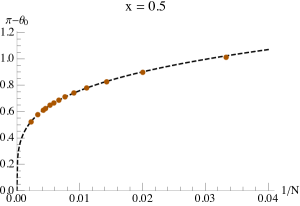
Figure 1: Finite $N$ solution of the discrete phase equation (8). Left: roots of (8) for $N=100$ drawn as phases on circles of different radii. The outmost circle has $x=0.5$, while the inner circles have $x$ increased in steps $0.05$ up to $x=0.9$. Right: gap half-width $\pi-\vartheta_{0}$ evaluated at $x=x_{\rm H}$ with increasing $N$ up to 450. The dashed line is a power law fit providing an exponent very close to $1/4$, i.e. $\vartheta_{0}(x_{\rm H})=\pi+\mathcal{O}(N^{-1/4})$.

As discussed in Raha:2017jgv , the determination of the saddle point $\bm{\vartheta}$ of (1) for finite $N$ amounts to finding the solution of the set of equations

$$\sum_{\ell\neq k}\cot\left(\frac{\vartheta_{k}-\vartheta_{\ell}}{2}\right)-\frac{4\,x\,(1+x^{2})\,\sin(\vartheta_{k}-\vartheta_{\ell})}{1+x^{4}-2\,x^{2}\,\cos(2\,(\vartheta_{k}-\vartheta_{\ell}))}=0.$$ (8)

The numerical solution of (8) for $N=100$ and $x>x_{\rm H}$ is shown in the left panel of Fig. (1) where one appreciates the opening of a gap whose width increases as $x\to 1$. The distribution of the roots $\bm{\vartheta}$ is non trivial, i.e. it is not uniform. Precisely at the $N=\infty$ Hagedorn transition point, $x=x_{\rm H}$, the gap closes as $N\to\infty$ according to the finite size scaling $\pi-\vartheta_{0}=\mathcal{O}\left(N^{-\delta}\right)$ with $\delta\simeq 1/4$, as shown in the right panel. This slow convergence of observables at increasing $N$ means that a reliable characterization of the model for $N=\infty$ is difficult by extrapolation from finite $N$ data. Besides, we are interested in analytical expansions near Hagedorn transition as well as at high temperature. For these reasons, we present in the next section a self-consistent accurate treatment of the $N=\infty$ limit that will prove itself to be more effective than finite $N$ extrapolation.

At $N\to\infty$, the roots of (8) are described by a smooth density $\rho(\vartheta;x)$ which is positive for $|\vartheta|<\vartheta_{0}(x)$ and vanishes at $\vartheta=\pm\vartheta_{0}$. Taking the continuum limit of (8), the function $\rho(\vartheta;x)$ obeys the homogeneous integral equation

$$\int_{-\vartheta_{0}(x)}^{\vartheta_{0}(x)}d\vartheta\,G(\vartheta^{\prime}-\vartheta;x)\,\rho(\vartheta;x)=0,$$

$$G(\vartheta;x)=\cot\left(\frac{\vartheta}{2}\right)-\frac{4\,x\,(1+x^{2})\,\sin\vartheta}{x^{4}+1-2\,x^{2}\,\cos(2\vartheta)}.$$ (9)

To solve it, we exploit the remarkably simple identity

$$\frac{x\,(1+x^{2})\,\sin\vartheta}{x^{4}+1-2\,x^{2}\,\cos(2\vartheta)}=\sum_{n=0}^{\infty}x^{2n+1}\,\sin((2n+1)\,\vartheta),$$ (10)

that holds in our case, i.e. for $0<x<1$ and real $\vartheta$. The expansion (10) allows to write (2) in the form

$$\int_{-\vartheta_{0}(x)}^{\vartheta_{0}(x)}d\vartheta\,\cot\left(\frac{\vartheta^{\prime}-\vartheta}{2}\right)\,\rho(\vartheta;x)=$$

$$\qquad\qquad 4\,\sum_{n=0}^{\infty}x^{2n+1}\,\int_{-\vartheta_{0}(x)}^{\vartheta_{0}(x)}d\vartheta\,\sin((2n+1)\,(\vartheta^{\prime}-\vartheta))\,\rho(\vartheta;x).$$ (11)

Taking into account that the density is expected to be even, $\rho(\vartheta;x)=\rho(-\vartheta;x)$, we can further simplify (2) and obtain

$$\int_{-\vartheta_{0}(x)}^{\vartheta_{0}(x)}d\vartheta\,\cot\left(\frac{\vartheta^{\prime}-\vartheta}{2}\right)\,\rho(\vartheta;x)=$$

$$\qquad\qquad 4\,\sum_{n=0}^{\infty}x^{2n+1}\,\sin((2n+1)\vartheta^{\prime})\,\int_{-\vartheta_{0}(x)}^{\vartheta_{0}(x)}d\vartheta\,\cos((2n+1)\,\vartheta)\,\rho(\vartheta;x).$$ (12)

It is convenient to recast (2) in the apparently inhomogeneous form

$$\int_{-\vartheta_{0}(x)}^{\vartheta_{0}(x)}d\vartheta\,\cot\left(\frac{\vartheta^{\prime}-\vartheta}{2}\right)\,\rho(\vartheta)=4\,\sum_{n=0}^{\infty}\rho_{n}\,x^{2n+1}\,\sin((2n+1)\vartheta^{\prime}),$$ (13)

where we have introduced the trigonometric momenta

$$\rho_{n}(x)=\int_{-\vartheta_{0}(x)}^{\vartheta_{0}(x)}d\vartheta\,\cos((2n+1)\,\vartheta)\,\rho(\vartheta;x).$$ (14)

As discussed in Aharony:2003sx , the general solution of the problem (13) is known and reads

$$\rho(\vartheta) =\frac{1}{\pi}\sqrt{\sin^{2}\left(\frac{\vartheta_{0}}{2}\right)-\sin^{2}\left(\frac{\vartheta}{2}\right)}\,\sum_{m=1}^{\infty}Q_{m}\,\cos\left[(m-\tfrac{1}{2})\,\vartheta\right],$$

$$Q_{m} =\mathop{\sum_{\ell=0}^{\infty}}_{\frac{m+\ell-1}{2}=0,1,2,\dots}4\,x^{m+\ell}\rho_{\frac{m+\ell-1}{2}}\,P_{\ell}(\cos\vartheta_{0}),$$ (15)

where, for brevity, we have omitted the explicit dependence on $x$. We can now truncate the expansion (2) by keeping only a fixed number of terms $\bm{\rho}^{(K)}=\{\rho_{k}\}_{k=0,\dots,K}$. The density is thus written in terms of the finite set of quantities $\bm{\rho}^{(K)}$. Replacing the density expression into (14) we obtain a homogeneous linear system

$$\mathcal{M}^{(K)}(x,\vartheta_{0}^{(K)})\,\bm{\rho}^{(K)}=0.$$ (16)

Non trivial solutions exists only if

$$\det\mathcal{M}^{(K)}(x,\vartheta_{0}^{(K)})=0,$$ (17)

which is the condition that determines the approximate gap width $\vartheta_{0}^{(K)}$ for each $x>x_{\rm H}$. Once $\vartheta_{0}^{(K)}$ is computed, we solve (16) for the eigenvector $\bm{\rho}^{(K)}$ and obtain the density from (2). The eigenvector normalization is fixed by requiring $\rho(\vartheta)$ to be normalized with unit integral. To appreciate the accuracy of the method, we show in Tab. (1) the solution $\vartheta_{0}^{(K)}(x)$ of (17) evaluated at various $x>x_{\rm H}$, and with $K$ growing from 10 to 34.

$$\begin{array}[]{cccccc}\hline\cr\hline\cr K&\phantom{xx}&\vartheta_{0}^{(K)}(0.6)&\vartheta_{0}^{(K)}(0.7)&\vartheta_{0}^{(K)}(0.8)&\vartheta_{0}^{(K)}(0.9)\\ \hline\cr 10&&0.7561179{\color[rgb]{1,0,0}8}&0.67837{\color[rgb]{1,0,0}211}&0.6173{\color[rgb]{1,0,0}5541}&0.526{\color[rgb]{1,0,0}88066}\\ 14&&0.75611796&0.678371{\color[rgb]{1,0,0}40}&0.61733{\color[rgb]{1,0,0}829}&0.5267{\color[rgb]{1,0,0}5452}\\ 18&&0.75611796&0.6783713{\color[rgb]{1,0,0}8}&0.617337{\color[rgb]{1,0,0}87}&0.5267{\color[rgb]{1,0,0}2285}\\ 22&&0.75611796&0.67837137&0.6173377{\color[rgb]{1,0,0}5}&0.5267{\color[rgb]{1,0,0}1194}\\ 26&&0.75611796&0.67837137&0.61733773&0.52670{\color[rgb]{1,0,0}810}\\ 30&&0.75611796&0.67837137&0.61733773&0.526706{\color[rgb]{1,0,0}91}\\ 34&&0.75611796&0.67837137&0.61733773&0.52670659\\ \hline\cr\hline\cr\end{array}$$

Table 1: Solution of the condition (17) for various $x>x_{\rm H}$ and increasing number of modes $K$. As a guide, we write in red the digits that change moving to the next row.

The convergence appears to be exponential in $K$ although with a decreasing rate as $x\to 1$. This is because the effect of the convergence factors $x^{2n+1}$ in (2) is reduced. Nevertheless, still at $x=0.9$, the accuracy is of about 6 digits for $K=34$.

Working out the prediction of the above algorithm in the interval $x_{\rm H}<x<1$ we obtain the black curve in Fig. (2) where we plot $\sin(\vartheta_{0}(x)/2)$ vs. $x$. To appreciate the convergence with $N$, we also show some sample points obtained at finite $N=20,50,100$ from the solution of (8). The dashed curves are analytical approximations valid around $x_{\rm H}$ and $x=1$ derived in the next section, i.e.

$$x \to x_{\rm H}:\qquad\sin\frac{\vartheta_{0}(x)}{2}=1-\sqrt{\frac{x-\frac{1}{2}}{2}}-\frac{1}{4}\left(x-\frac{1}{2}\right)+\dotsb,$$

$$x \to 1:\qquad\vartheta_{0}(x)=\left[6\,\pi\,(1-x)\right]^{1/3}+\dotsb.$$ (18)

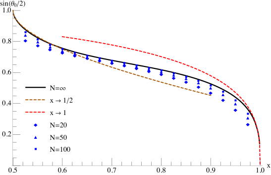
Figure 2: Temperature dependence of the phase gap $\vartheta_{0}(x)$. The black central curve is the result of the $N=\infty$ algorithm keeping $K=34$ modes. The blue symbols show the finite $N$ results at $N=20,50,100$ from the solution of (8). The dashed brown and red curves are the analytical approximations in (2).

As we shall discuss later, the self-consistent determination of $\rho(\vartheta)$ provides also analytical information near the Hagedorn transition. We shall see that only the first term in (2) survives. This shows that $\rho(\vartheta)$ is well described by

$$x\to x_{\rm H}:\qquad\rho(\vartheta;x)\to\frac{1}{\pi\,\sin^{2}(\vartheta_{0}/2)}\,\left(\sin^{2}\frac{\vartheta_{0}}{2}-\sin^{2}\frac{\vartheta}{2}\right)^{1/2}\,\cos\frac{\vartheta}{2},$$ (19)

which is Wigner semi-circle law in the variable $\sin(\vartheta/2)$, well known in the theory of random symmetric matrices. Strictly at $x=x_{\rm H}$ this reduces to $\rho(\vartheta;1/2)=\frac{1}{\pi}\,\cos^{2}\frac{\vartheta}{2}$. For $x\to 1$, we have found that the phase density is very well described by a quadratic law inside its support, i.e.

$$x\to 1:\qquad\rho(\vartheta;x)\to\frac{3}{4\,\vartheta_{0}^{3}}\,(\vartheta_{0}^{2}-\vartheta^{2}),$$ (20)

as will also be confirmed analytically in the next section. The limiting forms (19) and (20) are tested in Fig. (3). In the two panels, we show the exact density profile from the self-consistent algorithm and the predictions (19) and (20) at $x=0.501$ and $x=0.99$ respectively. The horizontal scale in the two panels is quite different due to the wide variation of $\vartheta_{0}(x)$. Up to a rescaling, the gross shape of the two densities is roughly similar, although the two regimes are clearly associated with different functions (semi-circle and quadratic).

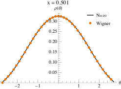
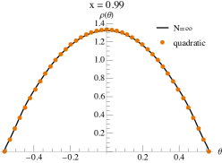
Figure 3: Temperature dependence of the phase density $\rho(\vartheta;x)$. Left: Just above the Hagedorn transition. The black line is the density obtained by plugging in (2) the solution of (17). The orange points are sample evaluations of (19) and superimpose quite well. Right: Near $x=1$. Again, the black line is the result from the self-consistent algorithm, while the orange points are samples of (20). Apart from the very ends of the distribution, the agreement is very good.

3 Analytical expansions

In this section, we derive the analytical expansions (17) characterizing the phase density $\rho(\vartheta;x)$ and its endpoint $\vartheta_{0}(x)$ near the Hagedorn transition and at very high temperature $x\to 1$.

3.1 Opening of the gap near the Hagedorn transition

The condition (17) may be solved perturbatively around $x=x_{\rm H}$. It is an algebraic equation in the variables $x$ and $h=\sin(\vartheta_{0}^{(K)}/2)$ whose complexity increases rapidly with $K$. Just to give an example, for the almost trivial case $K=1$ we have the constraint

$$K=1:\quad 1+2h^{2}\left(h^{2}-2\right)x=0.$$ (21)

The branch starting at $(x,h)=(1/2,1)$ has the expansion

$$K=1:\quad h=1-\left(\frac{x-x_{\rm H}}{2}\right)^{1/2}-\frac{1}{4}\,(x-x_{\rm H})+\frac{3}{2}\left(\frac{x-x_{\rm H}}{2}\right)^{3/2}+\dotsb.$$ (22)

For $K=2$, the condition (17) is much more complicated and reads

$$K=2:\quad 1+2h^{2}\left(h^{2}-2\right)x+2h^{2}\left(100h^{10}-312h^{8}+366h^{6}-200h^{4}+51h^{2}-6\right)x^{3}$$

$$+4h^{8}\left(25h^{8}-152h^{6}+288h^{4}-224h^{2}+64\right)x^{4}=0.$$ (23)

Expanding again around $x_{\rm H}$ we find

$$K=2:\quad h=1-\left(\frac{x-x_{\rm H}}{2}\right)^{1/2}-\frac{1}{4}\,(x-x_{\rm H})-\frac{33}{2}\left(\frac{x-x_{\rm H}}{2}\right)^{3/2}+\dotsb.$$ (24)

Repeating the procedure for increasing $K$, one finds that the first two terms of the expansion of $h$ are independent on $K$,

$$h=1-\left(\frac{x-x_{\rm H}}{2}\right)^{1/2}-\frac{1}{4}\,(x-x_{\rm H})+\text{c}^{(K)}\,\left(\frac{x-x_{\rm H}}{2}\right)^{3/2}+\dotsb.$$ (25)

while the values of the third coefficient are

$$c^{(K)}=\frac{3}{2},-\frac{33}{2},-\frac{199}{6},-\frac{793}{18},-\frac{76153}{1530},-\frac{2484163}{47430},-\frac{5915131}{110670},-\frac{32551537891}{604368870},\dotsb.$$ (26)

Increasing $K$ up to 30 and working with exact rational values, this sequence converges numerically to an asymptotic value that can be estimated by Wynn acceleration algorithm bender2013advanced . The results are quite stable and independent on the Wynn algorithm parameter and give $c^{(\infty)}=-54.0888227$. Such a large value suggests that the expansion (26) could be only asymptotic, as expected near a phase transition.

Plugging the expansion (26) in the linear system (16) one finds that all $\rho_{n>0}$ vanish linearly with $x-x_{\rm H}$. This leaves the semi-circle asymptotic density that we wrote in (19).

3.2 Density collapse at high temperature

The expansion in the high temperature regime $x\to 1$ is more complicated and cannot be obtained from the formalism of Section (2) because all $\rho_{n}$ have a non trivial limit. Nevertheless, we can check consistency of the quadratic density (20) by studying the $x\to 1$ limit of the integral equation (2). This is non trivial due to the $x$ dependence of $\vartheta_{0}(x)$. Analysis of the numerical data computed in Section (2) suggest that

$$\vartheta_{0}=\kappa\,(1-x)^{1/3}+\dotsb.$$ (27)

Actually, this Ansatz may be self-consistently checked in the following together with the determination of the amplitude $\kappa$. To this aim, the density can be rescaled

$$\rho(\vartheta)=\frac{1}{\vartheta_{0}}\widetilde{\rho}(\vartheta/\vartheta_{0}),\qquad\int_{-1}^{1}du\,\widetilde{\rho}(u)=1,$$ (28)

and the integral equation (2) can be written in the new variables

$$\int_{-1}^{1}du^{\prime}\bigg{[}\cot\left(\vartheta_{0}\,\frac{u-u^{\prime}}{2}\right)-\frac{4\,x\,(1+x^{2})\,\sin(\vartheta_{0}(u-u^{\prime})}{x^{4}+1-2\,x^{2}\,\cos(2\,\vartheta_{0}\,(u-u^{\prime}))}\bigg{]}\,\widetilde{\rho}(u^{\prime})=0.$$ (29)

Let us denote the kernel in the integral as $G(u;x)$, it is useful to plot it as a function of $u$ at various $x\to 1$ with the substitution $\vartheta_{0}\to\kappa\,(1-x)^{1/3}$. This is shown in the left panel of Fig. (4) where $\kappa=1$ to see what is going on. As $x\to 1$, the kernel splits into the sum of a linear background plus a $\delta^{\prime}(u)$ term which is localized in a region of width $\sim(1-x)^{2/3}$. The background part comes from the naive $x\to 1$ expansion of

$$G(u,x)=\cot\left(\kappa(1-x)^{1/3}\frac{u}{2}\right)-\frac{4\,x\,(1+x^{2})\,\sin(\kappa\,(1-x)^{1/3}\,u)}{x^{4}+1-2\,x^{2}\,\cos(2\,\kappa\,(1-x)^{1/3}\,u)}.$$ (30)

This gives

$$G(u,x)=-\frac{1}{2}\,\kappa\,u\,(1-x)^{1/3}+\dotsb,$$ (31)

which may be used for $|u|\gg(1-x)^{2/3}$. The second contribution comes from the integral (29) after a zooming associated with $u=(1-x)^{2/3}\,\xi$. At leading order, we get

$$\int_{-1}^{1}du^{\prime}\,G(u-u^{\prime};x)\,\widetilde{\rho}(u^{\prime}) =-2\,(1-x)^{1/3}\,\widetilde{\rho}\,^{\prime}(u)\,\int_{-\infty}^{\infty}d\xi\,\frac{1}{\kappa\,(1+\kappa^{2}\,\xi^{2})}+\dotsb$$

$$=-\frac{2\,\pi}{\kappa^{2}}\,(1-x)^{1/3}\,\widetilde{\rho}\,^{\prime}(u)+\dotsb,$$ (32)

which has indeed the form of a $\delta^{\prime}(u)$ contribution in the kernel. Consistency of the power $1/3$ in the $1-x$ factor in (31) and (3.2) is important to get a non trivial result and checks our scaling hypothesis. In summary, at this order in the $x\to 1$ expansion, the integral equation becomes simply

$$-\frac{1}{2}\,\kappa\,u-\frac{2\,\pi}{\kappa^{2}}\,\widetilde{\rho}\,^{\prime}(u)=0.$$ (33)

This gives both the quadratic density and the constant $\kappa$ in $\vartheta_{0}(x)$, see (27),

$$\widetilde{\rho}(u)=\frac{3}{4}\,(1-u^{2}),\qquad\kappa=(6\,\pi)^{1/3},$$ (34)

in agreement with (2) and (20).

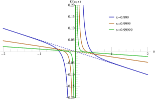
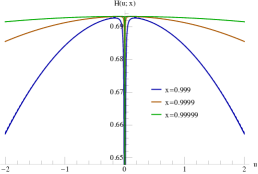
Figure 4: Detailed structure of some relevant integral kernels. Left: This panel shows the evaluation of the function $G$ defined in (30) and evaluated with $\kappa=1$. The plot shows that the kernel is composed of a linear background plus a singular part which is localized in a region of width $\sim(1-x)^{2/3}$ and approximates, as a distribution, a $\delta^{\prime}$ contribution. Right: This panel shows the evaluation of the function $H$ defined in (40). Similar to the left panel, we identify in the $x\to 1$ limit a quadratic background plus a narrow $\delta$ like contribution fully discussed in the text.

3.3 The transition order parameter

Further consistency checks of the derived aymptotic densities come from the analysis of the large $N$ behaviour of $\log Z_{0}$, i.e. the free energy up to trivial factors. The function $F_{2}(x)$ appearing as the leading term in the large $N$ expansion

$$\log Z_{0}=N^{2}\,F_{2}(x)+\mathcal{O}(N\log N),$$ (35)

can be computed from the density $\rho(\vartheta;x)$ as the double integral

$$F_{2}(x)=\frac{1}{2}\int_{-\vartheta_{0}(x)}^{\vartheta_{0}(x)}d\vartheta\,d\vartheta^{\prime}\,\log\bigg{[}4\,\sin^{2}\left(\frac{\vartheta-\vartheta^{\prime}}{2}\right)\,\frac{1+x^{2}+2\,x\,\cos(\vartheta-\vartheta^{\prime})}{1+x^{2}-2\,x\,\cos(\vartheta-\vartheta^{\prime})}\bigg{]}\,\rho(\vartheta)\,\rho(\vartheta^{\prime}).$$ (36)

As we mentioned in the introduction, the function $F_{2}(x)$ can be regarded as an order parameter for the Hagedorn transition. It is zero for $0<x<x_{\rm H}$ and increases monotonically for $x>x_{\rm H}$. The maximum value is attained at $x=1$ and is $F_{2}(1)=\log 2$. This follows from the exact relation Curtright:2017pfq

$$Z_{0}(x\to 1)=\left(\frac{2}{1-x}\right)^{N-1}\frac{R_{N}}{N!},$$ (37)

where $R_{N}$ is the number of labeled Eulerian digraphs with $N$ nodes. The asymptotic behaviour of $R_{N}$ has been recently computed in Curtright:2017pfq and reads

$$R_{N}\stackrel{{\scriptstyle N\to\infty}}{{\sim}}\left(\frac{2^{N}}{\sqrt{\pi N}}\right)^{N-1}\,e^{-1/4}\,\sqrt{N}\,\left[1+\frac{3}{16N}+\mathcal{O}(N^{-2})\right],$$ (38)

from which we get the term $N^{2}\,\log 2$ in $\log Z_{0}$.

Near the Hagedorn transition, we can evaluate $F_{2}(x)$ using the distribution (19). Direct expansion around $x=x_{\rm H}$ gives a leading linear behaviour

$$F_{2}(x)=\text{c}\,(x-x_{\rm H})+\dotsb,$$ (39)

where c is a constant that is obtained from a rather involved finite double integral. It can be safely extracted from the ratio $F_{2}(x_{\rm H}+\varepsilon)/\varepsilon$ as $\varepsilon\to 0$. Using $\varepsilon=0-10^{-3}$ and a fit of the form $a+b\,\sqrt{\varepsilon}$, we reproduce the numerical data very well with $\text{c}=1/2$ with a precision of one part in $10^{6}$. For this reason, we assume that this value of c is exact. A rather small range of values of $\varepsilon$ is needed suggesting again that the expansion around the Hagedorn temperature is only asymptotic. This is quite reasonable in this case because $F_{2}(x)$ is certainly not analytic at $x_{\rm H}$ – it is zero below the Hagedorn temperature and non zero above it. The linear behaviour (39) was originally predicted in Thorn:2015bia .

The computation of the leading correction to $F_{2}(x)$ for $x\to 1$ is more tricky and, again, it is again important to analyze in details the structure of the rescaled kernel with the leading order expression for $\vartheta_{0}$, i.e.

$$H(u;x)=\frac{\vartheta_{0}^{2}}{2}\,\log\bigg{[}4\,\sin^{2}\left(\vartheta_{0}\frac{u}{2}\right)\,\frac{1+x^{2}+2\,x\,\cos(\vartheta_{0}\,u)}{1+x^{2}-2\,x\,\cos(\vartheta_{0}\,u)}\bigg{]},\qquad\vartheta_{0}=\kappa\,(1-x)^{1/3}.$$ (40)

A plot of $H(u,x)$ as a function of $u$ with $x\to 1$ is shown in the right panel of Fig. (4). There is a naive quadratic contribution that comes from the direct expansion of $H$,

$$H(u;x)=\log 2-\frac{(3\,\pi)^{2/3}}{4\cdot 2^{1/3}}\,u^{2}\,(1-x)^{2/3}+\dotsb.$$ (41)

Integrating over $\vartheta$, $\vartheta^{\prime}$ in (36), this gives a first contribution to $F_{2}(x)$

$$F_{2}^{(a)}(x)=\log 2-\frac{(6\,\pi)^{2/3}}{20}\,(1-x)^{2/3}.$$ (42)

A second contribution comes from zooming in the region $u-u^{\prime}\sim(1-x)^{2/3}$ as in the previous section. This gives a second $\delta(u-u^{\prime})$-like contribution leading to

$$F_{2}^{(b)}(x)=\frac{3}{10}(1-x)^{2/3}\int_{-\infty}^{\infty}d\xi\log\left(\frac{\kappa^{2}\xi^{2}}{1+\kappa^{2}\xi^{2}}\right)=-\frac{3\pi}{5\kappa}\,(1-x)^{2/3}.$$ (43)

Summing (42) and (43), we obtain the expansion (7). In Fig. (5), we show the evaluation of (36) using the leading order density (20) with $\vartheta_{0}$ as in (2). We also show the approximation (7) as well as the exact numerical data points obtained in Raha:2017jgv . The agreement is remarkable despite the fact that we used the asymptotic density valid for $x\to 1$. This shows that $F_{2}(x)$ appears to be little dependent on the fine structure of the density itself. This is further confirmed by the fact that evaluation of $F_{2}(x)$ with the $x\to x_{\rm H}$ density or with the $x\to 1$ one are practically indistinguishable up to $x\simeq 0.9$.

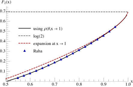
Figure 5: Evaluation of the order parameter $F_{2}(x)$. The black curve is the result of the evaluation of (36) using the asymptotic quadratic density in (20). Blue triangles are exact numerical data points taken from Raha:2017jgv . Finally, the brown dashed curve is the analytical approximation in (7).

4 Conclusions

In this paper we have considered the large $N$ thermodynamics of a simple $SU(N)$ string bit model devised to capture the tensionless limit of the associated string. The model lives in the color singlet sector and involves a projection implemented by a suitable group average, i.e. integration over $U\in SU(N)$. Dominant configurations are characterized by a non trivial density $\rho(\vartheta;T)$ of the $U$ invariant phases $\vartheta_{1},\dots,\vartheta_{N}$. We have analyzed the model in the gapped phase, i.e. for temperatures above the Hagedorn transition $T>T_{\rm H}$ where $\rho(\vartheta;T)$ is non zero only in the interval $|\vartheta|\leq\vartheta_{0}(T)<\pi$. By means of numerical and analytical tools, we have discussed in some details the temperature dependence of the phase density $\rho(\vartheta;T)$ including the gap endpoint $\vartheta_{0}(T)$. Our results provide quantitative information about the crossover from the low to high temperature phases in the considered model. It remains an open question to understand precisely which changes occur in models with more bits and if $1/N$ corrections are taken into account to resolve the phase transition. The corrections we found at $N=\infty$ contains non trivial power exponents, see (1) and (2). In particular, the phase density support $[-\vartheta_{0},\vartheta_{0}]$ opens a gap in the $\vartheta$ distribution of width $2\,(\pi-\vartheta_{0})\sim(T-T_{\rm H})^{1/4}$ near the Hagedorn transition. Besides, the support collapses with $\vartheta_{0}\sim T^{-1/3}$ for $T\gg T_{\rm H}$. It could be interesting to understand these relations in the context of a finite but large $N$ double scaling limit as in the Hagedorn transition for IIB string theory in an anti-de Sitter spacetime Liu:2004vy ; AlvarezGaume:2005fv .

References

- (1) R. Giles and C. B. Thorn, A Lattice Approach to String Theory, Phys. Rev. D16 (1977) 366.
- (2) C. B. Thorn, Reformulating string theory with the 1/N expansion, in The First International A.D. Sakharov Conference on Physics Moscow, USSR, May 27-31, 1991, pp. 0447–454, 1991. hep-th/9405069.
- (3) O. Bergman and C. B. Thorn, String bit models for superstring, Phys. Rev. D52 (1995) 5980–5996, [hep-th/9506125].
- (4) S. Sun and C. B. Thorn, Stable String Bit Models, Phys. Rev. D89 (2014) 105002, [1402.7362].
- (5) C. B. Thorn, Space from String Bits, JHEP 11 (2014) 110, [1407.8144].
- (6) G. Chen and S. Sun, Numerical Study of the Simplest String Bit Model, Phys. Rev. D93 (2016) 106004, [1602.02166].
- (7) R. Hagedorn, Statistical thermodynamics of strong interactions at high-energies, Nuovo Cim. Suppl. 3 (1965) 147–186.
- (8) G. ’t Hooft, A Planar Diagram Theory for Strong Interactions, Nucl. Phys. B72 (1974) 461.
- (9) C. B. Thorn, Infinite QCD at Finite Temperature: Is There an Ultimate Temperature?, Phys. Lett. 99B (1981) 458–462.
- (10) S. Fubini and G. Veneziano, Level structure of dual-resonance models, Nuovo Cim. A64 (1969) 811–840.
- (11) J. J. Atick and E. Witten, The Hagedorn Transition and the Number of Degrees of Freedom of String Theory, Nucl. Phys. B310 (1988) 291–334.
- (12) C. B. Thorn, String Bits at Finite Temperature and the Hagedorn Phase, Phys. Rev. D92 (2015) 066007, [1507.03036].
- (13) S. Raha, Hagedorn Temperature in Superstring Bits and SU(N) Characters, 1706.09951.
- (14) T. L. Curtright, S. Raha and C. B. Thorn, Color Characters for White Hot String Bits, 1708.03342.
- (15) P. Goddard, J. Goldstone, C. Rebbi and C. B. Thorn, Quantum dynamics of a massless relativistic string, Nucl. Phys. B56 (1973) 109–135.
- (16) G. ’t Hooft, Dimensional reduction in quantum gravity, in Salamfest 1993:0284-296, pp. 0284–296, 1993. gr-qc/9310026.
- (17) D. J. Gross and E. Witten, Possible Third Order Phase Transition in the Large N Lattice Gauge Theory, Phys. Rev. D21 (1980) 446–453.
- (18) O. Aharony, J. Marsano, S. Minwalla, K. Papadodimas and M. Van Raamsdonk, The Hagedorn - deconfinement phase transition in weakly coupled large N gauge theories, Adv.Theor.Math.Phys. 8 (2004) 603–696, [hep-th/0310285].
- (19) B. Sundborg, The Hagedorn transition, deconfinement and SYM theory, Nucl.Phys. B573 (2000) 349–363, [hep-th/9908001].
- (20) B. Skagerstam, On the Large Limit of the Color Quark - Gluon Partition Function, Z.Phys. C24 (1984) 97.
- (21) H. J. Schnitzer, Confinement/deconfinement transition of large N gauge theories with fundamentals: finite, Nucl. Phys. B695 (2004) 267–282, [hep-th/0402219].
- (22) H. J. Schnitzer, Confinement/deconfinement transition of large N gauge theories in perturbation theory with fundamentals: finite, hep-th/0612099.
- (23) S. H. Shenker and X. Yin, Vector Models in the Singlet Sector at Finite Temperature, 1109.3519.
- (24) M. Beccaria and A. A. Tseytlin, Partition function of free conformal fields in 3-plet representation, JHEP 05 (2017) 053, [1703.04460].
- (25) J. Jurkiewicz and K. Zalewski, Vacuum Structure of the Gauge Theory on a Two-dimensional Lattice for a Broad Class of Variant Actions, Nucl. Phys. B220 (1983) 167–184.
- (26) C. M. Bender and S. A. Orszag, Advanced mathematical methods for scientists and engineers I: Asymptotic methods and perturbation theory. Springer Science & Business Media, 2013.
- (27) H. Liu, Fine structure of Hagedorn transitions, hep-th/0408001.
- (28) L. Alvarez-Gaume, C. Gomez, H. Liu and S. Wadia, Finite temperature effective action, AdS5 black holes, and expansion, Phys. Rev. D71 (2005) 124023, [hep-th/0502227].