On the domain of Dirac and Laplace
type Operators on Stratified Spaces

Abstract.

We consider a generalized Dirac operator on a compact stratified space with an iterated cone-edge metric. Assuming a spectral Witt condition, we prove its essential self-adjointness and identify its domain and the domain of its square with weighted edge Sobolev spaces. This sharpens previous results where the minimal domain is shown only to be a subset of an intersection of weighted edge Sobolev spaces. Our argument does not rely on microlocal techniques and is very explicit. The novelty of our approach is the use of an abstract functional analytic notion of interpolation scales. Our results hold for the Gauss-Bonnet and spin Dirac operators satisfying a spectral Witt condition.

1. Introduction and statement of the main results

Singular spaces arise naturally in various parts of mathematics. Important examples of singular spaces include algebraic varieties and various moduli spaces; singular spaces also appear naturally as compactifications of smooth spaces or as limits of families of smooth spaces under controlled degenerations. The development of analytic techniques to study partial differential equations in the singular setting is a central issue in modern geometry.

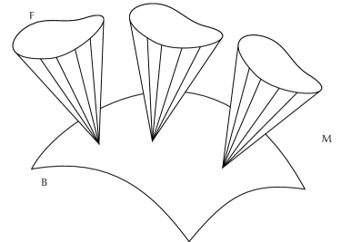
Figure 1. Simple Edge as a Cone bundle over $B$.

Cheeger [Che83] was the first to initiate an influential program on spectral analysis on smoothly stratified spaces with singular Riemannian metrics. Analysis of the associated geometric operators on spaces with conical singularities was the focal point of the research by Brüning and Seeley [BrSe85, BrSe87, BrSe91], Lesch [Les97], Melrose [Mel93], Schulze [Sch91, Sch94], Schrohe and Schulze [ScSc94, ScSc95], Gil, Krainer and Mendoza [GiMe03, GKM06] to name just a few.

Extensions to spaces with simple edge singularities were developed by Mazzeo [Maz91], as well as Schulze [Sch89, Sch02] and his collaborators, see also Gil, Krainer and Mendoza [GKM13]. Various questions in spectral geometry and index theory on spaces with simple edge singularities have been addressed e.g., by Brüning and Seeley [BrSe91], Mazzeo and Vertman [MaVe12, MaVe14], Krainer and Mendoza [KrMe16, KrMe15], Albin and Gell-Redman [AlGR16], Piazza and Vertman [PiVe16].

There have also been recent advances to lift the analysis to a very general setting of stratified spaces with iterated cone-edge singularities. Index theoretic questions for geometric Dirac operators on a general class of compact stratified Witt spaces with iterated cone-edge metrics have been studied by Albin, Leichtnam, Piazza and Mazzeo in [ALMP12, ALMP13, ALMP15]. The Yamabe problem on stratified spaces has been solved by Akutagawa, Carron and Mazzeo in [ACM14].

If we wish to go a step further and do spectral geometry on stratified spaces, the crucial difficulty appears already in the setting of a stratified space of depth two, illustrated as in Figure 2 below with fibers $F_{y}$, at each $y\in B=Y_{2}$, being simple edge spaces. Consider e.g., the family of Gauss–Bonnet operators on the fibers $F_{y},y\in B$. Even if we impose a spectral Witt condition so that the Gauss–Bonnet operators on the fibers are essentially self-adjoint, their domains may still vary with the base point across $B$. In case of variable domains however, smoothness of the operator family becomes a much more complicated issue, which needs to be resolved before any meaningful spectral geometric questions may be addressed.

Our main result is formulated using the concept of a spectral Witt condition and the weighted edge Sobolev space $\mathscr{H}^{1,1}_{e}(M)$ on a stratified Witt space $M$ with an iterated cone-edge metric, which will be made explicit below. Elements of the edge Sobolev spaces take values in a Hermitian vector bundle $E$, which is suppressed from the notation.

For the moment, the spectral Witt condition is a spectral gap condition on certain operators on fibers $F$, see Eq. (4.8) and Definition 10.2, and in case of the Gauss–Bonnet operator on a stratified Witt space it can always be achieved by scaling the iterated cone-edge metric appropriately. The weighted edge Sobolev space $\mathscr{H}^{s,\delta}_{e}(M)=\rho^{\delta}\mathscr{H}^{s}_{e}(M)$ is the Sobolev space $\mathscr{H}^{s}_{e}(M)$ of all square integrable sections of the Hermitian vector bundle $E$ that remain square integrable under weak application of $s\in\mathbb{N}$ edge vector fields, weighted with a $\delta$-th power of a smooth function $\rho$ that vanishes at the singular strata to first order. Our main theorem is now as follows.

Theorem 1.1.

Let $M$ be a compact stratified space with an iterated cone-edge metric. Let $D$ denote either the Gauss–Bonnet or the spin Dirac operator, and assume the spectral Witt condition holds, i.e., Definition 10.2. Then both $D$ and $D^{2}$ are essentially self-adjoint with domains

$$\begin{split}&\mathscr{D}_{\max}(D)=\mathscr{D}_{\min}(D)=\mathscr{H}^{1,1}_{e}(M),\\ &\mathscr{D}_{\max}(D^{2})=\mathscr{D}_{\min}(D^{2})=\mathscr{H}^{2,2}_{e}(M).\end{split}$$ (1.1)

In case of the Gauss–Bonnet operator, sections take values in the exterior algebra $\Lambda^{*}({}^{ie}T^{*}M)$ of the incomplete edge cotangent space $\Lambda^{*}({}^{ie}T^{*}M)$. In case of the spin Dirac operator, sections take values in the spinor bundle $S$.

Let us comment on related work in connection to Theorem 1.1. Gil, Krainer and Mendoza [GKM13, Theorem 4.2] prove that for an elliptic differential wedge operator $A$ of order $m$ on a simple edge space, under an assumption on indicial roots, $\mathscr{D}_{\min}(A)=\mathscr{H}^{m,m}_{e}(M)$. Our theorem here extends this statement to compact stratified spaces in the special case of the Gauss–Bonnet and Spin Dirac operators. Moreover, Albin, Leichtnam, Piazza and Mazzeo in [ALMP12, Prop. 5.9] prove that under the spectral Witt condition the minimal domain $\mathscr{D}_{\min}(D)$ of the Gauss–Bonnet operator is included in the intersection of $\mathscr{H}^{1,\delta}_{e}(M)$ for all $\delta<1$. Our theorem here sharpens this statement into an equality instead of an inclusion.

In addition we emphasize that we employ different methods which are more elementary and do have a functional analytic flavor. Furthermore we also do not need singular pseudo-differential calculi.

2. Smoothly stratified iterated edge spaces

In this section we recall basic aspects of the definition of a compact smoothly stratified space of depth $k\in\mathbb{N}_{0}$, referring the reader for a complete discussion e.g., to a very thorough analysis in [ALMP12, ALMP13, Alb16].

2.1. Smoothly stratified iterated edge spaces of depth zero and one

A compact stratified space of depth $k=0$ is simply a compact Riemannian manifold. A compact stratified space of depth $k=1$ is a compact simple edge space $\overline{M}$ with smooth open interior $M$, as discussed in e.g., in [Maz91, MaVe14]. More precisely, $\overline{M}$ admits a single stratum $B\subset\overline{M}$ which is a smooth compact manifold. The edge $B$ comes with an open tubular neighborhood $\mathscr{U}\subset\overline{M}$, a radial function $x$ defined on $\mathscr{U}$, and a smooth fibration $\phi:\mathscr{U}\to B$ with preimages $\phi^{-1}(q)\setminus\{q\}$, $q\in B$, being all diffeomorphic to open cones $C(F)=(0,1)\times F$ over a smooth compact manifold $F$. The restriction $x$ to each fiber $\phi^{-1}(q)$ is a radial function on that cone. We also write $\phi:{\partial}\mathscr{U}\to B$ for the fibration of the $\{x=1\}$ level set over $B$. The tubular neighborhood $\mathscr{U}\subset\overline{M}$ is illustrated in the Figure 1.

The resolution $\widetilde{M}$ is defined by replacing the cones in the tubular neighborhood $\mathscr{U}$ by finite cylinders $[0,1)\times F$. This defines a compact manifold with smooth boundary $\partial\widetilde{M}$ given by the total space of the fibration $\phi$. The resolution $\widetilde{\mathscr{U}}$ of the singular neighborhood $\mathscr{U}$ is defined analogously.

We equip the simple edge space with an edge metric $g$, which is smooth on $\overline{M}\setminus\mathscr{U}$ and which over $\mathscr{U}\backslash B$ takes the following form

$$g|_{\mathscr{U}}=dx^{2}+\phi^{\ast}g_{B}+x^{2}g_{F}+h=:g_{0}+h$$ (2.1)

where $g_{B}$ is a Riemannian metric on $B$, $g_{F}$ is a smooth family of bilinear forms on the tangent bundle of the total space of the fibration $\phi:{\partial}\mathscr{U}\to B$, restricting to a Riemannian metric on fibers $F$, $h$ is smooth on $\widetilde{\mathscr{U}}$ and $|h|_{g_{0}}=O(x)$, when $x\to 0$. We also require that $\phi:({\partial}\mathscr{U},g_{F}+\phi^{\ast}g_{B})\to(B,g_{B})$ is a Riemannian submersion.

Consider local coordinates $(x,y,\theta)$ on $\mathscr{U}\backslash B\subset M$ near the edge, where $x$ is as before the radial coordinate, $y$ is the lift of a local coordinate system on $B$ and $\theta$ restricts to local coordinates on each fiber $F$. Then, in terms of symmetric $2$-tensors $\textup{Sym}^{2}\{dx,xd\theta,dy\}$, generated by the $1$-tensors $\{dx,xd\theta,dy\}$, the higher order term $h$ satisfies over $\widetilde{\mathscr{U}}$

$$h\in x\cdot C^{\infty}(\widetilde{\mathscr{U}},\textup{Sym}^{2}\{dx,xd\theta,dy\}).$$ (2.2)

We finish with the standard definition of edge vector fields. The edge vector fields $\mathcal{V}_{e,1}$ are defined to be smooth on $\widetilde{M}$ and tangent to the fibers $F$ at $\partial\widetilde{M}$. We also write $\mathcal{V}_{ie,1}:=x^{-1}\mathcal{V}_{e,1}$, which we call the incomplete edge vector fields. In the chosen local coordinate system $(x,y,\theta)$ we have explicitly

$$\begin{split}&\mathcal{V}_{e,1}\restriction\widetilde{\mathscr{U}}=C^{\infty}(\widetilde{\mathscr{U}})\textup{- span}\,\{x\partial_{x},x\partial_{y_{1}},...,x\partial_{y_{\dim B}},\partial_{\theta_{1}},...,\partial_{\theta_{\dim F}}\},\\ &\mathcal{V}_{ie,1}\restriction\widetilde{\mathscr{U}}=C^{\infty}(\widetilde{\mathscr{U}})\textup{- span}\,\{\partial_{x},\partial_{y_{1}},...,\partial_{y_{\dim B}},x^{-1}\partial_{\theta_{1}},...,x^{-1}\partial_{\theta_{\dim F}}\}.\end{split}$$ (2.3)

2.2. Smoothly stratified iterated edge spaces of depth two

A stratified space of depth $2$ is modelled as above but allowing the links $F$ to be stratified spaces of depth $1$, with smooth links. This is illustrated in Figure 2, and we proceed with studying this case in detail to provide a basis for a definition of smoothly stratified iterated edge spaces of arbitrary depth.

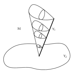
Figure 2. Tubular neighborhood $\mathscr{U}\subset\overline{M}$, $\overline{M}$ of depth $2$.

The fibration of cones with singular links defines an open edge space itself with an open edge singularity in $Y_{1}$, which fibers over $Y_{2}$ and contains $Y_{2}$ in its closure. We now have two strata $\{Y_{1},Y_{2}\}$ satisfying the following fundamental properties.

1. $Y_{2}\subset\overline{Y}_{1}$, and $Y_{2}$ is compact and smooth.

2. Any point $q\in Y_{1}=\overline{Y}_{1}\setminus Y_{2}$ has a tubular neighborhood of cones with smooth links. We say that $Y_{1}$ is a stratum of depth 1. Any point $q\in Y_{2}$ has a tubular neighborhood of cones $[0,1)\times F/_{(0,\theta_{1})\sim(0,\theta_{2})}$ with links $F$ being stratified spaces of depth $1$. We say that $Y_{2}$ is a stratum of depth $2$.

3. We have the following sequence of inclusions

   $$\overline{M}\supset\overline{Y}_{1}\supseteq Y_{2}\supseteq\varnothing.$$ (2.4)

   Then $\overline{M}\setminus\overline{Y}_{1}$ is an open Riemannian manifold dense in $\overline{M}$, and the strata of $\overline{M}$ are

   $$Y_{2},\;\;Y_{1}=\overline{Y}_{1}\setminus Y_{2},\;\;\overline{M}\setminus\overline{Y}_{1}.$$ (2.5)

The resolution $\widetilde{M}$ is defined as in the depth one case by replacing the cones in the fibration $\phi:\mathscr{U}\to Y_{2}$ by finite cylinders $[0,1)\times F$, and subsequently replacing the simple edge space $F$ with its resolution as well. This defines a compact manifold with corners. The resolution $\widetilde{\mathscr{U}}$ of $\mathscr{U}$ is defined analogously. We denote the radial function on each cone in the fibration $\phi$ by $x$, and write $x^{\prime}$ for the radial function of the simple edge space $F$.

We can now define an iterated cone-edge metric $g$ as before by specifying

$$g|_{\mathscr{U}}=dx^{2}+\phi^{\ast}g_{B}+x^{2}g_{F}+h=:g_{0}+h,$$ (2.6)

where $B=Y_{2}$, $g_{B}$ is a smooth Riemannian metric, $g_{F}$ restricting on the links $F$ to iterated cone-edge metrics of depth $1$ (simple edge space). As before, these metrics $g_{B}$ and $g_{F}$ do not depend on the radial function $x$, and the higher order terms of the metric are included in the tensor $h$, which is smooth on $\widetilde{\mathscr{U}}$ with $|h|_{g_{0}}=O(x)$ as $x\to 0$. We require that $\phi\restriction{\partial}\mathscr{U}:({\partial}\mathscr{U},g_{F}+\phi^{\ast}g_{B})\to(B,g_{B})$ is a Riemannian submersion and put the same condition on the fibers $(F,g_{F})$.

The edge vector fields $\mathcal{V}_{e,2}$, as well as the incomplete edge vector fields $\mathcal{V}_{ie,2}$, are defined similarly to $\mathcal{V}_{e,1}$ and $\mathcal{V}_{ie,1}$.

$$\begin{split}&\mathcal{V}_{e,2}\restriction\widetilde{\mathscr{U}}=C^{\infty}(\widetilde{\mathscr{U}})\textup{- span}\,\{(xx^{\prime})\partial_{x},(xx^{\prime})\partial_{y_{1}},...,(xx^{\prime})\partial_{y_{\dim B}},\mathcal{V}_{e,1}(F)\},\\ &\mathcal{V}_{ie,2}\restriction\widetilde{\mathscr{U}}=C^{\infty}(\widetilde{\mathscr{U}})\textup{- span}\,\{\partial_{x},\partial_{y_{1}},...,\partial_{y_{\dim B}},(xx^{\prime})^{-1}\mathcal{V}_{e,1}(F)\}.\end{split}$$ (2.7)

where $\mathcal{V}_{e,1}(F)$ refers to the edge vector fields on the simple edge space $F$.

2.3. Smoothly stratified iterated edge spaces of arbitrary depth

At an informal level we can now say that $\overline{M}$ is a compact smoothly stratified iterated edge space of arbitrary depth $k\geq 2$ with strata $\{Y_{\alpha}\}_{\alpha\in A}$ if $\overline{M}$ is compact and the following, inductively defined, properties are satisfied.

1. If $Y_{\alpha}\cap\overline{Y}_{\beta}\neq\varnothing$ then $Y_{\alpha}\subset\overline{Y}_{\beta}$ (each stratum is identified with its open interior).

2. The depth of a stratum $Y$ is the largest $(j-1)\in\mathbb{N}_{0}$ such that there exists a chain of pairwise distinct strata $Y=Y_{j},\;Y_{j-1},\ldots,Y_{1}$ with $Y_{i}\subset\overline{Y}_{i-1}$ for all $2\leq i\leq j$.

3. The stratum of maximal depth is smooth and compact. The maximal depth of any stratum of $\overline{M}$ is called the depth of $\overline{M}$.

4. Any point of $Y_{\alpha}$, a stratum of depth $j$, has a tubular neighborhood of cones with links being stratified spaces of depth $j-1$, for all $1\leq j\leq k$.

5. Setting

   $$\overline{M}=X_{n}\supset X_{n-1}=X_{n-2}\supseteq X_{n-3}\supseteq\cdots\supseteq X_{1}\supseteq X_{0},$$ (2.8)

   where $X_{j}$ is the union of all strata of dimension less or equal than $j$, $X_{n}\setminus X_{n-2}$ is an open Riemannian manifold, dense in $\overline{M}$.

We call the union $X_{n-2}$ of all $Y_{\alpha}$, for $\alpha\in A$ the singular part of $\overline{M}$, and its complement in $\overline{M}$ the regular part, denoted by $M$. The precise definition of smoothly stratified spaces contains some other technical conditions, cf. Thom–Mather-spaces [Alb16].

The resolution $\widetilde{M}$ is a manifold with corners defined iteratively by resolving in each step the highest codimension singular strata as before. Each tubular neighborhood $\mathscr{U}_{\alpha}$ of any point in $Y_{\alpha}$ admits a resolution $\widetilde{\mathscr{U}}_{\alpha}$ in an analogous way.

We define an iterated cone-edge metric $g$ on $M$ by asking $g$ to be an arbitrary smooth Riemannian metric away from singular strata, and requiring in each tubular neighborhood $\mathscr{U}_{\alpha}$ of any point in $Y_{\alpha}$ to have the following form

$$g|_{\mathscr{U}_{\alpha}}=dx^{2}+\phi^{\ast}_{\alpha}g_{Y_{\alpha}}+x^{2}g_{F_{\alpha}}+h=:g_{0}+h,$$ (2.9)

where $\phi_{\alpha}:\mathscr{U}_{\alpha}\to\phi_{\alpha}(\mathscr{U}_{\alpha})\subseteq Y_{\alpha}$ is the obvious fibration, $\phi_{\alpha}(\mathscr{U}_{\alpha})$ is open in $Y_{\alpha}$, the restriction $g_{Y_{\alpha}}\restriction\phi_{\alpha}(\mathscr{U}_{\alpha})$ is a smooth Riemannian metric, $g_{F}$ is a symmetric two tensor on the level set $\{x=1\}$, whose restriction to the links $F_{\alpha}$ (smoothly stratified iterated edge spaces of depth at most $(k-1)$) is an iterated cone-edge metric. The higher order term $h$ is smooth on $\widetilde{\mathscr{U}}_{\alpha}$ and satisfies $|h|_{g_{0}}=O(x)$, when $x\to 0$. We also assume that $\phi_{\alpha}\restriction{\partial}\mathscr{U}_{\alpha}:({\partial}\mathscr{U}_{\alpha},g_{F_{\alpha}}+\phi^{\ast}_{\alpha}g_{Y_{\alpha}})\to(\phi_{\alpha}(\mathscr{U}_{\alpha}),g_{Y_{\alpha}})$ is a Riemannian submersion and put the same condition in the lower depth. Existence of such smooth iterated cone-edge metrics is discussed in [ALMP12, Prop. 3.1].

The definition of edge vector fields $\mathcal{V}_{e,k}$ and incomplete edge vector fields $\mathcal{V}_{ie,k}$, extends to the smoothly stratified space $M$ by an inductive procedure as in case of $k=2$, cf. (2.7). To be precise, denote by $\rho$ a smooth function on the resolution $\widetilde{M}$, nowhere vanishing in its open interior, and vanishing to first order at each boundary face. Then $\mathcal{V}_{e,k}=\rho\mathcal{V}_{ie,k}$ and

$$\begin{split}&\mathcal{V}_{e,k}\restriction\widetilde{\mathscr{U}}=C^{\infty}(\widetilde{\mathscr{U}})\textup{- span}\,\{\rho\partial_{x},\rho\partial_{s_{1}},...,\rho\partial_{s_{\dim Y_{\alpha}}},\mathcal{V}_{e,k-1}(F_{\alpha})\},\\ &\mathcal{V}_{ie,k}\restriction\widetilde{\mathscr{U}}=C^{\infty}(\widetilde{\mathscr{U}})\textup{- span}\,\{\partial_{x},\partial_{s_{1}},...,\partial_{s_{\dim Y_{\alpha}}},\rho^{-1}\mathcal{V}_{e,k-1}(F_{\alpha})\}.\end{split}$$ (2.10)

2.4. Sobolev spaces on smoothly stratified iterated edge spaces

We may now define the edge Sobolev spaces in the setup of a compact stratified space $M$ of depth $k$ with an iterated cone-edge metric. Let ${}^{ie}TM$ denote the canonical vector bundle defined by the condition that the incomplete edge vector fields $\mathcal{V}_{ie,k}$ form locally a spanning set of sections $\mathcal{V}_{ie,k}=C^{\infty}(M,{}^{ie}TM)$. We denote by ${}^{ie}T^{*}M$ the dual of ${}^{ie}TM$, also referred to as the incomplete edge cotangent bundle. We write $E=\Lambda^{*}({}^{ie}T^{*}M)$, when discussing the Gauss–Bonnet operator, and we set $E$ to be the spinor bundle, when discussing the spin Dirac operator. In either of these cases we define the edge Sobolev spaces with values in $E$ as follows.

Definition 2.1.

Let $M$ be a compact smoothly stratified iterated edge space of arbitrary depth $k\in\mathbb{N}$ with an iterated cone-edge metric $g$. We denote by $L^{2}(M,E)$ the $L^{2}$ completion of smooth compactly supported differential forms $C^{\infty}_{0}(M,E)$. Denote by $\rho$ a smooth function on the resolution $\widetilde{M}$, nowhere vanishing in its open interior, and vanishing to first order at each boundary face. Then, for any $s\in\mathbb{N}$ and $\delta\in\mathbb{R}$ we define the weighted edge Sobolev spaces by

$$\begin{split}&\mathscr{H}_{e}^{s}(M):=\{\mathrm{\omega}\in L^{2}(M)\mid V_{1}\circ\cdots\circ V_{s}\mathrm{\omega}\in L^{2}(M,E),\ \textup{for}\ V_{j}\in\mathcal{V}_{e,k}\},\\ &\mathscr{H}_{e}^{s,\delta}(M):=\{\mathrm{\omega}=\rho^{\delta}u\mid u\in\mathscr{H}_{e}^{s}(M)\},\end{split}$$ (2.11)

where $V_{1}\circ\cdots\circ V_{s}\mathrm{\omega}\in L^{2}(M,E)$ is understood in the distributional sense.

3. Interpolation scales of Hilbert Spaces

3.1. Preliminaries

Let $H_{1},H_{2}$ be Hilbert spaces which are assumed to be embedded into a barrelled locally convex topological vector space, such that it makes sense to talk about $H_{1}+H_{2}$ (non-direct sum space) and $H_{1}\cap H_{2}$. Let $[H_{1},H_{2}]_{\theta}$, $0\leq\theta\leq 1$, be their complex interpolation space. For Calderón’s complex interpolation theory [Cal64] we refer to [Tay11, Sec. 4.2]. The space of bounded linear operators between $H_{1},H_{2}$ is denoted by $\mathscr{L}(H_{1},H_{2})$, resp. if $H_{1}=H_{2}=H$ we just write $\mathscr{L}(H)$.

If $H_{2}\hookrightarrow H_{1}$ is densely embedded such that the norm of $H_{2}$ is the graph norm of the nonnegative self-adjoint operator $\Lambda$ in $H_{1}$, then by [Tay11, Prop. 2.2]

$$[H_{1},H_{2}]_{\theta}=\mathscr{D}(\Lambda^{\theta}).$$ (3.1)

In fact, there is a converse to this statement.

Lemma 3.1.

Let $T:H_{1}\to H_{2}$ be a bounded operator between Hilbert spaces $H_{1}$ and $H_{2}$. Then we have the equality of ranges $\operatorname{ran}T=\operatorname{ran}\sqrt{T\ T^{*}}$.

• Let $T^{*}=U|T^{*}|=U\sqrt{T\ T^{\ast}}$ be the polar decomposition of $T^{*}$; $U$ is a partial isometry with $\operatorname{ran}U=\overline{\operatorname{ran}T^{*}}=(\ker T)^{\perp}$ and $\ker U=\ker T^{*}=(\operatorname{ran}T)^{\perp}$. Then, taking adjoints $T=\sqrt{T\ T^{*}}\ U^{*}$, and hence $\operatorname{ran}\sqrt{T\ T^{\ast}}\supset\operatorname{ran}T$. Since $\operatorname{ran}U^{*}=(\ker U)^{\perp}=(\ker T^{*})^{\perp}=(\ker\sqrt{T\ T^{*}})^{\perp}$, the equality follows. ∎

Proposition 3.2 ([LiMa72, Sec. I.2.1]).

Let $H$ be a Hilbert space with a dense subspace $\mathscr{D}\subset H$. Assume that $\mathscr{D}$ carries a Hilbert space structure such that the inclusion map $i:\mathscr{D}\hookrightarrow H$ is continuous. Then $\mathscr{D}=\operatorname{ran}\sqrt{i\ i^{*}}$ and $\sqrt{i\ i^{*}}:H\to\mathscr{D}$ is a unitary isomorphism. $\Lambda:=(\sqrt{i\ i^{*}})^{-1}$ is a self-adjoint operator with domain $\mathscr{D}$, hence

$$[H,\mathscr{D}]_{\theta}=\mathscr{D}(\Lambda^{\theta}),\;\theta\in[0,1].$$ (3.2)

• By (3.1), see [Tay11, Proposition 2.2], the last claim follows once the claims about the operator $\Lambda$ are established. From Lemma 3.1 we know that $\mathscr{D}=\operatorname{ran}\sqrt{i\ i^{*}}$. Note that $\ker i=\{0\}$, $\overline{\operatorname{ran}i}=H$ and hence $i^{*}$ and $\sqrt{i\ i^{*}}$ are injective with dense range. Consequently, $\Lambda=(\sqrt{i\ i^{*}})^{-1}$ is self-adjoint with domain $\mathscr{D}$. For $y\in\mathscr{D}$ we find

  $$\|\sqrt{i\ i^{*}}\ y\|_{\mathscr{D}}^{2} =\langle\sqrt{i\ i^{*}}\ y,\sqrt{i\ i^{*}}\ y\rangle_{\mathscr{D}}=\langle i^{*}\Lambda\ y,\sqrt{i\ i^{*}}\ y\rangle_{\mathscr{D}}$$ (3.3)

  $$=\langle\Lambda\ y,i\ \sqrt{i\ i^{*}}\ y\rangle_{H}=\langle y,\Lambda\ \sqrt{i\ i^{*}}\ y\rangle_{H}=\|y\|^{2}_{H}.$$

  Since $\mathscr{D}$ is dense the claim follows. ∎

3.2. Scales of Hilbert Spaces

From Brüning and Lesch [BrLe01, Section 2] we recall the useful concept of a scale of Hilbert spaces, which has been used in various forms by several authors, see Connes and Moscovici [CoMo95, Appendix B], Higson [Hig06, §4], Otgonbayar [Otg09] and Paycha [Pay10]. Let $H$ be a Hilbert space and $A$ a self-adjoint operator in $H$. Then

$$H^{\infty}:=\bigcap_{n=0}^{\infty}\mathscr{D}(|A|^{n})=\bigcap_{n=0}^{\infty}\mathscr{D}(A^{n})$$ (3.4)

is dense in $H$. For $s\in\mathbb{R}$, let $H^{s}(A)$ be the completion of $H^{\infty}$ with respect to the scalar product

$$\langle x,y\rangle_{s}:=\langle(I+A^{2})^{\frac{s}{2}}\ x,(I+A^{2})^{\frac{s}{2}}\ y\rangle.$$ (3.5)

Then $H^{n}(A)=\mathscr{D}(A^{n})=\mathscr{D}(|A|^{n})$ for $n\in\mathbb{Z}_{+}$, respectively, $H^{s}(A)=\mathscr{D}(|A|^{s})$, for any $s\geq 0$.

The properties of the family $\{H^{s}\}_{s\in\mathbb{R}}$ are reminiscent of properties of Sobolev spaces and they are summarized in the following proposition.

Proposition 3.3.

The family $(H^{s}(A))_{s\geq 0}$ satisfies:

1. $H^{s}$ is a Hilbert space, for all $s\geq 0$.

2. For $s^{\prime}\geq s$ we have a continuous embedding $H^{s^{\prime}}\hookrightarrow H^{s}$.

3. $[H_{s},H_{t}]_{\theta}=H_{\theta t+(1-\theta)s}$, for $0\leq\theta\leq 1$,
   in the sense of complex interpolation.

4. $H^{\infty}=\bigcap\limits_{s\geq 0}H^{s}$ is dense in $H^{t}$ for each $t$.

An abstract family $(H^{s})_{s\geq 0}$ of Hilbert spaces satisfying (1)–(4) is called an (interpolation) scale of Hilbert spaces. If there exists a self-adjoint operator $A$ such that $H^{s}=H^{s}(A)$ for $s\geq 0$ then we call $A$ a generator of the scale. The item (4) implies that $H^{s^{\prime}}$ is dense in $H^{s}$ for $s^{\prime}\geq s$. Proposition 3.2 implies that for $N>0$ there exists a self-adjoint operator $\Lambda\geq 0$ with $\mathscr{D}(\Lambda^{N})=H^{N}$ and hence $H^{s}=\mathscr{D}(\Lambda^{s})=:H^{s}(\Lambda)$ for $0\leq s\leq N$.

Remark 3.4.

Given a scale $(H^{s})_{s\geq 0}$ of Hilbert spaces as in Proposition 3.3, one may ask whether there exists a generator $\Lambda$, such that $H^{s}=\mathscr{D}(\Lambda^{s})$ for all $s\geq 0$, and not only for $0\leq s\leq N$.

We believe that in general the answer is no. E.g., the scale of Sobolev spaces $H^{s}([0,\infty))$ does not have a natural generator, although we cannot prove that there does not exist one. We leave this open question to the reader. This does not affect the discussion below.

Nonetheless, in the sequel we will for convenience assume that the scales do have a global generator $\Lambda$. As the arguments will always only concern a compact set of $s$-values, in light of the discussion above, this is not really a loss of generality.

Thus for all practical purposes we may think of a Hilbert space scale being the scale of a positive operator $\Lambda$. We note that if two positive self-adjoint operators $\Lambda_{1}$, $\Lambda_{2}$ have the same domain $\mathscr{D}(\Lambda_{1})=\mathscr{D}(\Lambda_{2})$ then $H^{1}(\Lambda_{1})=H^{1}(\Lambda_{2})$, and by complex interpolation

$$\mathscr{D}(\Lambda_{1}^{s})=[H,H^{1}(\Lambda_{1})=H^{2}(\Lambda_{2})]_{s}=\mathscr{D}(\Lambda_{2}^{s}),\;{\text{for}}\;0\leq s\leq 1.$$ (3.6)

In general, however, we will have

$$\mathscr{D}(\Lambda_{1}^{s})\not=\mathscr{D}(\Lambda_{2}^{s}),\;\text{for}\;s>1.$$ (3.7)

Example 3.5.

To illustrate this by example consider

$$\Lambda_{1}:=\left(\begin{array}[]{cc}0&\partial_{x}\\ -\partial_{x}&0\end{array}\right),\quad\Lambda_{2}:=\left(\begin{array}[]{cc}0&\partial_{x}+a\\ -\partial_{x}+a&0\end{array}\right),$$ (3.8)

acting in the Hilbert space $L^{2}(\mathbb{R}_{+},\mathbb{C}^{2})=L^{2}(\mathbb{R}_{+})\otimes\mathbb{C}^{2}$ with domain

$$\mathscr{D}(\Lambda_{1})=\mathscr{D}(\Lambda_{2})=\bigl{\{}f={f_{1}\choose f_{2}}\in H^{1}(\mathbb{R}_{+})\otimes\mathbb{C}^{2}\,\bigm{|}\,f_{1}(0)=0\bigr{\}}.$$ (3.9)

It is straightforward to see that $\Lambda_{j},j=1,2$ are self-adjoint. However, the domains of the squares are given by

$$\begin{split}\mathscr{D}(\Lambda_{1}^{2})&=\bigl{\{}f\in H^{2}(\mathbb{R}_{+})\otimes\mathbb{C}^{2}\,\bigm{|}\,f_{1}(0)=0,\ f_{2}^{\prime}(0)=0\bigr{\}},\\ \mathscr{D}(\Lambda_{2}^{2})&=\bigl{\{}f\in H^{2}(\mathbb{R}_{+})\otimes\mathbb{C}^{2}\,\bigm{|}\,f_{1}(0)=0,\ f_{2}^{\prime}(0)+a\cdot f_{2}(0)=0\bigr{\}},\end{split}$$ (3.10)

thus $H^{s}(\Lambda_{1})\not=H^{s}(\Lambda_{2})$ for $1<s\leq 2$.

In view of Example 3.5, we may now ask for criteria such that two self-adjoint operators generate the same interpolation scale.

Definition 3.6.

Let $\Lambda$ be a self-adjoint operator in the Hilbert space $H$ with interpolation scale $H^{s}(\Lambda)_{s\geq 0}$. A linear operator $P:H^{\infty}(\Lambda)\to H^{\infty}(\Lambda)$ is said to be of order $\mu$ if $P$ admits a formal adjoint with respect to the scalar product of $H$, and for any $s\in\mathbb{R}$, $P$ and $P^{t}$ extend by continuity $H^{s}(\Lambda)\to H^{s-\mu}(\Lambda)$. I. e. there are constants $C_{s}(P),C_{s}(P^{t})$ such that for $x\in H^{\infty}$ we have $\|Px\|_{s-\mu}\leq C_{s}(P)\cdot\|x\|_{s}$ and $\|P^{t}x\|_{s-\mu}\leq C_{s}(P)\cdot\|x\|_{s}$. By $\operatorname{Op}^{\mu}(\Lambda)$ we denote the operators of order $\mu$.

Clearly, $\operatorname{Op}^{\bullet}(\Lambda)=\bigcup_{\mu}\operatorname{Op}^{\mu}(\Lambda)$ is a filtered algebra of operators acting on $H^{\infty}(\Lambda)$. To show that an operator $P$ is of order $\mu$ it suffices to check the estimates in the definition on a sequence $(t_{j})_{j}$ of $t$-values with $\lim t_{j}=\infty$. This follows again from complex interpolation.

The continuity condition can equivalently be formulated in terms of the resolvent of $\Lambda$:

(3.11)

Here, the lower arrow is given by the operator

$$(I+|\Lambda|)^{t-\mu}\circ P\circ(I+|\Lambda|)^{-t},$$ (3.12)

which is required to be bounded on $H$ for all $t\in\mathbb{R}$. If $P=\Lambda_{2}$ is a selfadjoint operator of order $1$ on the Sobolev-scale $H^{\bullet}(\Lambda_{1})$, then we have an equality of interpolation scales $H^{\bullet}(\Lambda_{1})=H^{\bullet}(\Lambda_{2})$, and hence we conclude using the interpolation property with the following observation.

Proposition 3.7.

Assume that for any $n\in\mathbb{N}\setminus\{0\}$

$$(I+|\Lambda_{1}|)^{n-1}\circ\Lambda_{2}\circ(I+|\Lambda_{1}|)^{-n}$$ (3.13)

is bounded on $H$. Then $\Lambda_{1}$ and $\Lambda_{2}$ generate the same interpolation scales. If (3.13) is bounded only for $n=1$ then we can only infer that $H^{s}(\Lambda_{1})=H^{s}(\Lambda_{2})$ for $0\leq s\leq 1$.

3.3. Tensor products of interpolation scales

In this section we follow in part [BrLe01, Sec. 2]. We fix two interpolation scales $\{H_{j}^{s}\}_{s\geq 0}$, $j=1,2$ with generators $\Lambda_{1}$, $\Lambda_{2}$. Without loss of generality we may choose $\Lambda_{1}$, $\Lambda_{2}$ such that they are greater or equal to $I$ and hence we may define the scalar product on $H_{j}^{s}$ by

$$\langle x,y\rangle_{H^{s}_{j}}:=\langle\Lambda_{j}^{s}x,\Lambda_{j}^{s}y\rangle_{H_{j}}.$$ (3.14)

For tensor products of (unbounded) operators we refer to the Appendix A, in particular Proposition A.2. $H_{1}\hat{\otimes}H_{2}$ resp. $A\hat{\otimes}B$ denotes the completed Hilbert space tensor product resp. the tensor product of (unbounded) operators $A,B$.

Lemma 3.8.

$\{H_{1}^{s}\hat{\otimes}H^{s}_{2}\}_{s\geq 0}$ is an interpolation scale with generator $\Lambda_{1}\hat{\otimes}\Lambda_{2}$.

• By Proposition A.3, we have $\Lambda_{1}\hat{\otimes}\Lambda_{2}\geq I$, hence the graph norm of $(\Lambda_{1}\hat{\otimes}\Lambda_{2})^{s}$ is equivalent to $\|(\Lambda_{1}\hat{\otimes}\Lambda_{2})^{s}x\|$. Note furthermore, that $\Lambda_{1}\hat{\otimes}I$ and $I\hat{\otimes}\Lambda_{2}$ are commuting self-adjoint operators greater or equal to $I$, thus

  $$(\Lambda_{1}\hat{\otimes}\Lambda_{2})^{s}=(\Lambda_{1}\hat{\otimes}I\cdot I\hat{\otimes}\Lambda_{2})^{s}=\Lambda^{s}_{1}\hat{\otimes}I\cdot I\hat{\otimes}\Lambda_{2}^{s}=\Lambda^{s}_{1}\hat{\otimes}\Lambda_{2}^{s}.$$ (3.15)

  Furthermore, for $x_{j}\in H_{1}^{\infty}$, $y_{j}\in H_{2}^{\infty},j=1,\ldots,r$ we have with each summation index running from $j=1,\ldots,r$:

  $$\Bigl{\|}\sum_{j}x_{j}\otimes y_{j}\Bigr{\|}^{2}_{H_{1}^{s}\hat{\otimes}H_{2}^{s}} =\sum_{k,l}\langle x_{k}\otimes y_{k},x_{l}\otimes y_{l}\rangle_{H_{1}^{s}\hat{\otimes}H_{2}^{s}}$$

  $$=\sum_{k,l}\langle x_{k},x_{l}\rangle_{H_{1}^{s}}\langle y_{k},y_{l}\rangle_{H_{2}^{s}}$$

  $$=\sum_{k,l}\langle\Lambda_{1}^{s}x_{k},\Lambda_{1}^{s}x_{l}\rangle_{H_{1}}\langle\Lambda_{2}^{s}y_{k},\Lambda_{2}^{s}y_{l}\rangle_{H_{2}}$$

  $$=\Bigl{\langle}\Lambda_{1}^{s}\hat{\otimes}\Lambda_{2}^{s}\Bigl{(}\sum_{j}x_{j}\otimes y_{j}\Bigr{)},\Lambda_{1}^{s}\hat{\otimes}\Lambda_{2}^{s}\Bigl{(}\sum_{j}x_{j}\otimes y_{j}\Bigr{)}\Bigr{\rangle}_{H_{1}\otimes H_{2}}.$$

  This shows that the tensor product norm on $H_{1}^{s}\hat{\otimes}H_{2}^{s}$ is equivalent to the graph norm of $\Lambda_{1}^{s}\hat{\otimes}\Lambda_{2}^{s}$ which proves the claim. ∎

As a consequence we get for $s,t\geq 0$

$$\bigl{[}H_{1}^{s}\hat{\otimes}H_{2}^{s},H_{1}^{t}\hat{\otimes}H_{2}^{t}\bigr{]}_{\theta}=H_{1}^{\theta t+(1-\theta s)}\hat{\otimes}H_{2}^{\theta t+(1-\theta)s}=[H_{1}^{s},H_{1}^{t}]_{\theta}\hat{\otimes}[H_{2}^{s},H_{2}^{t}]_{\theta}.$$ (3.16)

Since every interpolation pair of Hilbert spaces may be embedded into an interpolation scale (Proposition 3.2) we obtain

Corollary 3.9.

If $E^{\prime}\subset E$, $F^{\prime}\subset E$ are interpolation pairs of Hilbert spaces then, for $0\leq\theta\leq 1$,

$$[E\hat{\otimes}F,E^{\prime}\hat{\otimes}F^{\prime}]_{\theta}=[E,E^{\prime}]_{\theta}\hat{\otimes}[F,F^{\prime}]_{\theta}.$$ (3.17)

Remark 3.10.

The tensor product of Lemma 3.8 should not be confused with the Sobolev spaces on product spaces. Note that on $\mathbb{R}^{n}$ we have $H^{s}(\mathbb{R}^{n})=H^{s}(\Delta_{\mathbb{R}^{n}})$, where $\Delta_{\mathbb{R}^{n}}=-\sum_{j=1}^{n}\partial_{x_{j}}^{2}$ is the Laplace operator. Now it is not true that

$$H^{s}(\mathbb{R}^{n}\times\mathbb{R}^{m})=H^{s}(\mathbb{R}^{n})\hat{\otimes}H^{s}(\mathbb{R}^{m}).$$ (3.18)

Rather we have the following equalities

$$H^{s}(\mathbb{R}^{n}\times\mathbb{R}^{m}) =H^{s}(\Delta_{\mathbb{R}^{n}\times\mathbb{R}^{m}}=\Delta_{\mathbb{R}^{n}}\hat{\otimes}I+I\hat{\otimes}\Delta_{\mathbb{R}^{m}})$$ (3.19)

$$\stackrel{{\scriptstyle!}}{{=}}H^{s}(\Delta_{\mathbb{R}^{n}})\hat{\otimes}L^{2}(\mathbb{R}^{m})\ \cap\ L^{2}(\mathbb{R}^{n})\hat{\otimes}H^{s}(\mathbb{R}^{m}),\;\text{ for }s\geq 0.$$

This is due to the equality of domains

$$\mathscr{D}((\Delta_{\mathbb{R}^{n}}\hat{\otimes}I+I\hat{\otimes}\Delta_{\mathbb{R}^{m}})^{s})=\mathscr{D}(\Delta^{s}_{\mathbb{R}^{n}}\hat{\otimes}I)\cap\mathscr{D}(I\hat{\otimes}\Delta^{s}_{\mathbb{R}^{m}}),$$ (3.20)

as we will see below.

Definition 3.11.

Given two interpolation scales $\{H^{s}_{j}\}_{s\geq 0},j=1,2$, we put for $s\geq 0$

$$\mathscr{H}^{s}:=\mathscr{H}^{s}(\{H_{1}^{\bullet}\},\{H_{2}^{\bullet}\}):=H_{1}^{s}\hat{\otimes}H_{2}^{0}\cap H_{1}^{0}\hat{\otimes}H_{2}^{s}.$$ (3.21)

This is a Hilbert space with scalar product being the sum of the scalar products of $H_{1}^{s}\hat{\otimes}H_{2}^{0}$ and $H_{1}^{0}\hat{\otimes}H_{2}^{s}$.

Proposition 3.12.

Let $\Lambda_{1},\Lambda_{2}\geq I$ be generators of $\{H_{1}^{\bullet}\}$, $\{H_{2}^{\bullet}\}$, respectively. Then $\{\mathscr{H}^{s}\}_{s\geq 0}$ is an interpolation scale with generator $\Lambda_{1}\hat{\otimes}I+I\hat{\otimes}\Lambda_{2}$ and

$$\mathscr{H}^{s}=\bigcap_{0\leq t\leq s}H_{1}^{t}\hat{\otimes}H_{2}^{s-t}=\left(H_{1}^{s}\hat{\otimes}H_{2}^{0}\right)\cap\left(H_{1}^{0}\hat{\otimes}H_{2}^{s}\right).$$ (3.22)

• Recall that $\Lambda_{1}\hat{\otimes}I$, $I\hat{\otimes}\Lambda_{2}$ are commuting self-adjoint operators greater or equal to $I$. Now from

  $$\frac{1}{2}(b^{s}+c^{s})\leq(b+c)^{s}\leq 2^{s}(b^{s}+c^{s}),$$ (3.23)

  for $b,c,s\geq 0$ and the Spectral Theorem we infer

  $$\mathscr{H}^{s}=\mathscr{D}(\Lambda_{1}^{s}\hat{\otimes}I)\cap\mathscr{D}(I\hat{\otimes}\Lambda_{2}^{s})=\mathscr{D}((\Lambda_{1}\hat{\otimes}I+I\hat{\otimes}\Lambda_{2})^{s}),$$ (3.24)

  hence the first part of the statement follows.

  For the second part, we first note that the concavity of the $\log$–function implies the inequality

  $$a^{\theta}\cdot b^{1-\theta}\leq\theta\cdot a+(1-\theta)\cdot b,$$ (3.25)

  for $a,b\geq 0$ and $0\leq\theta\leq 1$. For the commuting operators $\Lambda_{1}\hat{\otimes}I$, $I\hat{\otimes}\Lambda_{2}$ and $0\leq\theta\leq 1$ the inequality implies

  $$H_{1}^{0}\hat{\otimes}H_{2}^{s}\cap H_{1}^{s}\hat{\otimes}H_{2}^{0} =\mathscr{D}(I\hat{\otimes}\Lambda_{2}^{s})\cap\mathscr{D}(\Lambda_{1}^{s}\hat{\otimes}I)$$ (3.26)

  $$\subset\mathscr{D}((\Lambda_{1}^{s}\hat{\otimes}I)^{\theta}\cdot(I\hat{\otimes}\Lambda_{2}^{s})^{1-\theta})$$

  $$=\mathscr{D}(\Lambda_{1}^{\theta s}\hat{\otimes}\Lambda_{2}^{s-\theta s})=H_{1}^{\theta s}\hat{\otimes}H_{2}^{s-\theta s}.$$

  Consequently, $\mathscr{H}^{s}\subset\bigcap_{0\leq t\leq s}H_{1}^{t}\hat{\otimes}H_{2}^{s-t}$. ∎

4. Dirac operators on an abstract edge

4.1. Generalized Dirac operators on an abstract edge

Let $S$ be a smooth family of self-adjoint operators in a Hilbert space $H$ with parameter $y\in\mathbb{R}^{b}$ and a fixed domain $\mathscr{D}_{S}$. We assume that each $S(y)$ is discrete. A generalized Dirac Operator $D$ acting on $C_{0}^{\infty}(\mathbb{R}_{+}\times\mathbb{R}^{b},H^{\infty})$ is defined by the following (differential) expression

$$D:=\Gamma(\partial_{x}+X^{-1}S)+T,$$ (4.1)

where $x\in\mathbb{R}_{+}$, $X$ denotes the multiplication operator by $X$, $\Gamma$ is skew-adjoint and a unitary operator on the Hilbert space $L^{2}(\mathbb{R}_{+}\times\mathbb{R}^{b},H)$, and $T$ is a symmetric generalized Dirac Operator on $\mathbb{R}^{b}$, given in terms of coordinates $(y_{1},\ldots,y_{b})\in\mathbb{R}^{b}$ and smooth families $(c_{1}(y),c_{b}(y))$ of bounded linear operators on $H$, which satisfy Clifford relations for each fixed $y\in\mathbb{R}^{b}$, by

$$T=\sum_{j=1}^{b}c_{j}(y)\frac{\partial}{\partial y_{j}}.$$ (4.2)

Here, we have hid the vector bundle value action of the Dirac Operator $T$ into the Hilbert space $H$.

We assume that the following standard commutator relations hold

$$\Gamma\ S+S\ \Gamma =0,$$ (4.3)

$$\Gamma\ T+T\ \Gamma =0,$$

$$T\ S-S\ T =0.$$

In §4.5 we show that the Gauss–Bonnet operator on a simple edge satisfies these relations, cf. (4.25). The same relations hold for the spin Dirac operator, as shown in [AlGR16, (3.16), (3.18)].

We shall also consider $D$ with coefficients frozen at some $y_{0}\in\mathbb{R}^{b}$

$$D_{y_{0}}:=\Gamma(\partial_{x}+X^{-1}S(y_{0}))+T_{y_{0}},\quad\textup{where}\ T_{y_{0}}=\sum_{j=1}^{b}c_{j}(y_{0})\frac{\partial}{\partial y_{j}}.$$ (4.4)

Consider the Fourier transform $\mathfrak{F}_{y\to\xi}$ on the $L^{2}(\mathbb{R}^{b})$-component of $L^{2}(\mathbb{R}_{+}\times\mathbb{R}^{b},H)$. We use Hörmander’s normalization and write

$$\left(\mathfrak{F}_{y\to\xi}f\right)(\xi)=\int_{\mathbb{R}^{b}}e^{-i\langle y,\xi\rangle}f(y)dy,\quad\left(\mathfrak{F}^{-1}_{y\to\xi}g\right)(y)=\int_{\mathbb{R}^{b}}e^{i\langle y,\xi\rangle}g(\xi)\frac{d\xi}{(2\pi)^{b}}.$$ (4.5)

We compute

$$\mathfrak{F}_{y\to\xi}\circ D_{y_{0}}\circ\mathfrak{F}_{y\to\xi}^{-1}=\Gamma(\partial_{x}+X^{-1}S(y_{0}))+ic(\xi;y_{0})=:L(y_{0},\xi),$$ (4.6)

where

$$c(\xi;y_{0}):=\sum_{j=1}^{b}c_{j}(y_{0})\xi_{j}.$$ (4.7)

The usual strategy is now to study invertibility of $L(y_{0},\xi)$ on appropriate spaces, which is then used to construct the parametrix for $D$ and analysis of its domain.

4.2. The spectral Witt condition

We also impose a spectral Witt condition, which asserts that

$$\forall\,y\in\mathbb{R}^{b}:\ \operatorname{Spec}S(y)\cap\left[-1,1\right]=\varnothing,$$ (4.8)

Remark 4.1.

We should point out that Albin and Gell-Redman [AlGR16] require a smaller spectral gap $\operatorname{Spec}S(y)\cap\Bigl{(}-1/2,1/2\Bigr{)}=\varnothing$. However, when proving an analogue of the crucial [AlGR16, Lemma 3.10] by explicit computations, it seems that a smaller spectral gap may not be sufficient for our purposes. In any case, if $D$ is the Gauss–Bonnet operator on a stratified Witt space, one can always achieve $\operatorname{Spec}S(y)\cap\Bigl{(}-R,R\Bigr{)}=\varnothing$ for any $R>0$ by a simple rescaling of the metric.

4.3. Squares of generalized Dirac operators

In view of the commutator relations (4.3), the generalized Laplace operators $D^{2}$ and $D_{y_{0}}^{2}$, acting both on $C_{0}^{\infty}(\mathbb{R}_{+}\times\mathbb{R}^{b},H^{\infty})$, are of the following form

$$\begin{split}&D^{2}=-{\partial}_{x}^{2}+X^{-2}\ S\ (S+1)+T^{2},\\ &D^{2}_{y_{0}}=-{\partial}_{x}^{2}+X^{-2}\ S(y_{0})\ (S(y_{0})+1)+T^{2}_{y_{0}}.\end{split}$$

We set $A:=\left|S\right|+\frac{1}{2}$. Assuming $\operatorname{Spec}S\cap\left[-1,1\right]=\varnothing$, we find $S(S+1)=A^{2}-1/4$ and rewrite the generalized Laplacians $D^{2}$ and $D_{y_{0}}^{2}$ as follows

$$\begin{split}&D^{2}=-{\partial}_{x}^{2}+X^{-2}\Bigl{(}A^{2}-\frac{1}{4}\Bigr{)}+T^{2},\\ &D^{2}_{y_{0}}=-{\partial}_{x}^{2}+X^{-2}\Bigl{(}A^{2}(y_{0})-\frac{1}{4}\Bigr{)}+T^{2}_{y_{0}}.\end{split}$$

As before, we may apply the Fourier transform $\mathfrak{F}_{y\to\xi}$ and compute

$$\begin{split}\mathfrak{F}_{y\to\xi}\circ D^{2}_{y_{0}}\circ\mathfrak{F}_{y\to\xi}^{-1}&=-{\partial}_{x}^{2}+X^{-2}\left(A^{2}(y_{0})-\frac{1}{4}\right)+c(\xi,y_{0})^{2}\\ &=:L^{2}(y_{0},\xi),\ \textup{where}\ c(\xi;y_{0})^{2}=-\sum_{j,k=1}^{b}c_{j}(y_{0})c_{k}(y_{0})\xi_{j}\xi_{k}.\end{split}$$

4.4. Sobolev-spaces of an abstract edge

Recall the definition of interpolation scales of Hilbert spaces in §3. This defines for each $y_{0}\in\mathbb{R}^{b}$ an interpolation scale $H^{s}(S(y_{0}))$, $s\in\mathbb{R}$. We can now define the Sobolev-scales on the model cone and the model edge in our abstract setting. Consider for this the Sobolev-scale $H^{\bullet}_{e}(\mathbb{R}_{+})$ generated by $(ix\partial_{x}+i/2)$; and the Sobolev-scale $H_{e}^{\bullet}(\mathbb{R}_{+}\times\mathbb{R}^{b})$ generated by $\Lambda=(ix\partial_{x}+i/2)\hat{\otimes}I+I\hat{\otimes}xT_{y_{0}}$. The lower index $e$ indicates that these interpolation scales coincide with the edge Sobolev spaces for integer orders.

Definition 4.2.

Let $y_{0}\in\mathbb{R}^{b}$ be fixed.

1. The Sobolev-scale $W^{\bullet}(\mathbb{R}_{+},H)$ of an abstract model cone is defined as an interpolation scale with generator $(ix\partial_{x}+i/2)\hat{\otimes}I+I\hat{\otimes}S(y_{0})$. By Proposition 3.12

   $$W^{s}(\mathbb{R}_{+},H):=(H^{s}_{e}(\mathbb{R}^{+})\hat{\otimes}H)\cap(L^{2}(\mathbb{R}_{+})\hat{\otimes}H^{s}(S(y_{0}))).$$ (4.9)

2. The Sobolev-scale $W^{\bullet}(\mathbb{R}_{+}\times\mathbb{R}^{b},H)$ of an abstract model edge is defined as an interpolation scale with generator $\Lambda\hat{\otimes}I+I\hat{\otimes}S(y_{0})$, where $\Lambda$ is the generator of the Sobolev-scale $H^{s}_{e}(\mathbb{R}_{+}\times\mathbb{R}^{b})$. By Proposition 3.12

   $$W^{s}(\mathbb{R}_{+}\times\mathbb{R}^{b},H):=(H^{s}_{e}(\mathbb{R}_{+}\times\mathbb{R}^{b})\hat{\otimes}H)\cap(L^{2}(\mathbb{R}_{+}\times\mathbb{R}^{b})\hat{\otimes}H^{s}(S(y_{0}))).$$ (4.10)

Remark 4.3.

In view of Proposition 3.7, for $y,y_{0}\in\mathbb{R}^{b}$, the interpolation scales of $S(y)$ and $S(y_{0})$ need not coincide. However, since for any $y\in\mathbb{R}^{b}$, the domain of $S(y)$ is fixed and given by $\mathscr{D}_{S}$, we have $H^{s}(S(y))=H^{s}(S(y_{0}))$ for $0\leq s\leq 1$. In particular the Sobolev scales $W^{s}(\mathbb{R}_{+},H)$ and $W^{s}(\mathbb{R}_{+}\times\mathbb{R}^{b},H)$ do not depend on $y_{0}\in\mathbb{R}^{b}$ for $0\leq s\leq 1$. In fact, in our arguments below we will require independence of the Sobolev spaces for $0\leq s\leq 2$.

We conclude with a definition of weighted Sobolev-spaces, where we denote by $X$ the multiplication operator by $x\in\mathbb{R}_{+}$.

Definition 4.4.

The weighted Sobolev-scales are defined by

$$W^{s,\delta,l}:=X^{\delta}(1+X)^{-l}W^{s}(\mathbb{R}_{+},H),\quad W^{s,\delta}:=W^{s,\delta,0}.$$ (4.11)

4.5. Examples of generalized Dirac operators on an abstract edge

The spin Dirac operator on a model edge space is indeed a generalized Dirac operator in the sense that it is given by the differential expression (4.1) and satisfies the commutator relations (4.3). This has been established by Albin and Gell-Redman [AlGR16]. In this subsection we prove that the Gauss–Bonnet operator on a model edge space is a generalized Dirac operator in the sense above as well.

Let $M^{m}$ and $N^{n}$ be Riemannian manifolds. Given forms $\omega_{p}\in\Omega^{p}(M)$ and $\eta_{q}\in\Omega^{q}(N)$, we will write $\omega_{p}\wedge\eta_{q}$ for the form $\pi_{M}^{*}(\omega_{p})\wedge\pi_{N}^{*}(\eta_{q})\in\Omega^{p+q}(M\times N)$, where $\pi_{M}:M\times N\to M$ and $\pi_{N}:M\times N\to N$ are projections onto the first and second factors respectively. It is well known that the exterior derivative $d:\Omega^{\ast}(M\times N)\to\Omega^{\ast}(M\times N)$ satisfies the Leibniz rule, i.e., if $\omega_{p}\in\Omega^{p}(M)$ and $\eta_{q}\in\Omega^{q}(N)$ then

$$d(\omega_{p}\wedge\eta_{q})\ =\ (d^{M}\omega_{p})\wedge\eta_{q}+(-1)^{p}\ \omega_{p}\wedge(d^{N}\eta_{q}).$$ (4.12)

Lemma 4.5.

The same Leibniz rule holds for the adjoint of the exterior derivative $d^{t}$ in $\Omega^{\ast}(M\times N)$.

• Note that $\Omega^{\ast}(M\times N)$ can be decomposed into a direct sum of subspaces of the form $\Omega^{\ast}(M)\wedge\Omega^{\ast}(N)$. Hence it suffices to study the action of $d^{t}$ on differential forms in $\Omega^{p+1}(M)\wedge\Omega^{q}(N)$, where we have

  $$d^{t}:\Omega^{p+1}(M)\wedge\Omega^{q}(N)\to(\Omega^{p}(M)\wedge\Omega^{q}(N))\oplus(\Omega^{p}(M)\wedge\Omega^{q-1}(N)).$$ (4.13)

  Consider $\widetilde{\omega}_{p}\in\Omega^{p}(M)$, $\omega_{p+1},\widetilde{\omega}_{p+1}\in\Omega^{p+1}(M)$, $\widetilde{\eta}_{q},\eta_{q}\in\Omega^{q}(N)$ and $\widetilde{\eta}_{q-1}\in\Omega^{q-1}(N)$, then we have for the first component of $d^{t}$

  $$\langle d_{p+q}^{t}(\omega_{p+1}\wedge \eta_{q}),\widetilde{\omega}_{p}\wedge\widetilde{\eta}_{q}\rangle$$ (4.14)

  $$=\langle\omega_{p+1}\wedge\eta_{q},(d^{M}\widetilde{\omega}_{p})\wedge\widetilde{\eta}_{q}+(-1)^{p}\widetilde{\omega}_{p}\wedge(d^{N}\widetilde{\eta}_{q})\rangle$$

  $$=\langle\omega_{p+1}\wedge\eta_{q},(d^{M}\widetilde{\omega}_{p})\wedge\widetilde{\eta}_{q}\rangle$$

  $$=\langle\omega_{p+1},(d^{M}\widetilde{\omega}_{p})\rangle_{M}\langle\eta_{q},\widetilde{\eta}_{q}\rangle_{N}$$

  $$=\langle(d^{M,t}\omega_{p+1}),\widetilde{\omega}_{p}\rangle_{M}\langle\eta_{q},\widetilde{\eta}_{q}\rangle_{N}$$

  $$=\langle(d^{M,t}\omega_{p+1})\wedge\eta_{q},\widetilde{\omega}_{p}\wedge\widetilde{\eta}_{q}\rangle.$$

  For the second component of $d^{t}$, we obtain

  $$\langle d_{p+q}^{t} (\omega_{p+1}\wedge\eta_{q}),\widetilde{\omega}_{p+1}\wedge\widetilde{\eta}_{q-1}\rangle$$ (4.15)

  $$=\langle\omega_{p+1}\wedge\eta_{q},(d^{M}\widetilde{\omega}_{p+1})\wedge\widetilde{\eta}_{q-1}+(-1)^{p+1}\widetilde{\omega}_{p+1}\wedge(d^{N}\widetilde{\eta}_{q-1})\rangle$$

  $$=(-1)^{p+1}\langle\omega_{p+1}\wedge\eta_{q},\widetilde{\omega}_{p+1}\wedge(d^{N}\widetilde{\eta}_{q-1})\rangle$$

  $$=(-1)^{p+1}\langle\omega_{p+1},\widetilde{\omega}_{p+1}\rangle_{M}\langle\eta_{q},(d^{N}\widetilde{\eta}_{q-1})\rangle_{N}$$

  $$=(-1)^{p+1}\langle\omega_{p+1},\widetilde{\omega}_{p+1}\rangle_{M}\langle(d^{N,t}\eta_{q}),\widetilde{\eta}_{q-1}\rangle_{N}$$

  $$=(-1)^{p+1}\langle\omega_{p+1}\wedge(d^{N,t}\eta_{q}),\widetilde{\omega}_{p+1}\wedge\widetilde{\eta}_{q-1}\rangle.$$

  Altogether, we arrive at the result

  $$d_{p+q}^{t}(\omega_{p+1}\wedge\eta_{q})=(d_{p}^{M,t}\omega_{p+1})\wedge\eta_{q}+(-1)^{p+1}\omega_{p+1}\wedge(d^{N,t}_{q}\eta_{q}).$$ (4.16)

  ∎

We now apply Lemma 4.5 to the case of a model edge $C(F)\times Y$ of cones $C(F)=\mathbb{R}_{+}\times F$ fibered over an edge manifold $Y$. Recall that on a cone $C(F)=\mathbb{R}_{+}\times F$ we have as in [BrSe88, (5.9a), (5.9b)] the following isometric identifications

$$\Omega^{\rm ev}(C(F))\cong C^{\infty}(\mathbb{R}_{+},\Omega^{\ast}(F)),\qquad\Omega^{\rm odd}(C(F))\cong C^{\infty}(\mathbb{R}_{+},\Omega^{\ast}(F)).$$ (4.17)

Under these identifications the Gauss–Bonnet operator $D=d+d^{t}$ acting now from $\Omega^{\rm ev}(C(F))\cong C^{\infty}(\mathbb{R}_{+},\Omega^{\ast}(F))$ to $\Omega^{\rm odd}(C(F))\cong C^{\infty}(\mathbb{R}_{+},\Omega^{\ast}(F))$, takes the form cf. [BrSe88, (5.10)]

$$D=\frac{d}{dx}+X^{-1}A.$$ (4.18)

Respectively, the full operator $D$ acts on $C^{\infty}(\mathbb{R}_{+},\Omega^{\ast}(C(F))\oplus\Omega^{\ast}(C(F)))$ as

$$\left(\begin{array}[]{cc}0&-\frac{d}{dx}+X^{-1}A\\ \frac{d}{dx}+X^{-1}A&0\end{array}\right)=\left(\begin{array}[]{cc}0&-1\\ 1&0\end{array}\right)\left(\frac{d}{dx}+X^{-1}\left(\begin{array}[]{cc}A&0\\ 0&-A\end{array}\right)\right).$$ (4.19)

Note that the grading operator on $\Omega^{\ast}(C(F))\oplus\Omega^{\ast}(C(F))$ is $\left(\begin{array}[]{cc}1&0\\ 0&-1\end{array}\right)$.

Taking now the cartesian product by a manifold $Y$ (the edge), we have

$$\Omega^{\rm ev}(C(F)\times Y) =\Omega^{\rm ev}(C(F))\otimes\Omega^{\rm ev}(Y)\oplus\Omega^{\rm odd}(C(F))\otimes\Omega^{\rm odd}(Y)$$

$$\cong C^{\infty}(\mathbb{R}_{+},\Omega^{\ast}(F))\otimes\Omega^{\rm ev}(Y)\oplus C^{\infty}(\mathbb{R}_{+},\Omega^{\ast}(F))\otimes\Omega^{\rm odd}(Y),$$

where we used the identifications (4.17) in the second equality. In exactly the same manner we find for differential forms of odd degree

$$\Omega^{\rm odd}(C(F)\times Y) =\Omega^{\rm odd}(C(F))\otimes\Omega^{\rm ev}(Y)\oplus\Omega^{\rm ev}(C(F))\otimes\Omega^{\rm odd}(Y)$$

$$\cong C^{\infty}(\mathbb{R}_{+},\Omega^{\ast}(L))\otimes\Omega^{\rm ev}(Y)\oplus C^{\infty}(\mathbb{R}_{+},\Omega^{\ast}(F))\otimes\Omega^{\rm odd}(Y).$$

So again we have an identification of the space $\Omega^{\rm ev}(C(F)\times Y)$ with the space $\Omega^{\rm odd}(C(F)\times Y)$. For $\omega_{1}\in\Omega^{\rm ev}(C(F))$, $\omega_{2}\in\Omega^{\rm odd}(C(F))$, $\eta_{1}\in\Omega^{\rm ev}(Y)$ and $\eta_{2}\in\Omega^{\rm odd}(Y)$, we have $\omega_{1}\otimes\eta_{1}\oplus\omega_{2}\otimes\eta_{2}\in\Omega^{\rm ev}(C(F)\times Y)$. Using Lemma 4.5 we now find for $D=d+d^{t}$,

$$D(\omega_{1}\otimes\eta_{1}\oplus\omega_{2}\otimes\eta_{2}) =D^{C(F)}\omega_{1}\otimes\eta_{1}+\omega_{1}\otimes D^{Y}\eta_{1}$$ (4.20)

$$+D^{C(F)}\omega_{2}\otimes\eta_{2}-\omega_{2}\otimes D^{Y}\eta_{2}$$

$$=\left(\begin{array}[]{cc}\partial_{x}+X^{-1}A&-D^{Y}\\ D^{Y}&-\partial_{x}+X^{-1}A\end{array}\right)\left(\begin{array}[]{c}\omega_{1}\otimes\eta_{1}\\ \omega_{2}\otimes\eta_{2}\end{array}\right).$$

Note that by construction $A$ and $D^{Y}$ commute. By abuse of notation $A$ acts as $A\otimes I$ and $D^{Y}$ acts as $I\otimes D^{Y}$ on the tensors. The full Gauss–Bonnet then becomes

$$D=\left(\begin{array}[]{cccc}0&0&-\partial_{x}+X^{-1}A&D^{Y}\\ 0&0&-D^{Y}&\partial_{x}+X^{-1}A\\ \partial_{x}+X^{-1}A&-D^{Y}&0&0\\ D^{Y}&-\partial_{x}+X^{-1}A&0&0\end{array}\right).$$ (4.21)

This expression can rewritten as follows.

$$D=\left(\begin{array}[]{cccc}0&0&-1&0\\ 0&0&0&1\\ 1&0&0&0\\ 0&-1&0&0\end{array}\right) \left(\partial_{x}+X^{-1}\left(\begin{array}[]{cccc}1&0&0&0\\ 0&-1&0&0\\ 0&0&-1&0\\ 0&0&0&1\end{array}\right)\cdot A\right)$$ (4.22)

$$+\left(\begin{array}[]{cccc}0&0&0&1\\ 0&0&-1&0\\ 0&-1&0&0\\ 1&0&0&0\end{array}\right)\cdot D^{Y},$$

with grading operator $\left(\begin{array}[]{cc}I_{2}&0\\ 0&-I_{2}\end{array}\right)$ where $I_{2}$ is the identity in $M_{2}(\mathbb{R})$. Define the following matrices

$$\Gamma=\left(\begin{array}[]{cccc}0&0&-1&0\\ 0&0&0&1\\ 1&0&0&0\\ 0&-1&0&0\end{array}\right)\!\!,S=\left(\begin{array}[]{cccc}1&0&0&0\\ 0&-1&0&0\\ 0&0&-1&0\\ 0&0&0&1\end{array}\right)A,T=\left(\begin{array}[]{cccc}0&0&0&1\\ 0&0&-1&0\\ 0&-1&0&0\\ 1&0&0&0\end{array}\right)D^{Y}\!.$$

We introduce the usual Clifford matrices

$$\sigma_{1}=\left(\begin{array}[]{cc}0&-1\\ 1&0\end{array}\right),\ \sigma_{2}=\left(\begin{array}[]{cc}0&i\\ i&0\end{array}\right),\ \omega=\left(\begin{array}[]{cc}1&0\\ 0&-1\end{array}\right)=i\cdot\sigma_{1}\cdot\sigma_{2}.$$ (4.23)

We have,

$$\Gamma =\left(\begin{array}[]{cc}0&-\omega\\ \omega&0\end{array}\right)=\sigma_{1}\otimes\omega,$$ (4.24)

$$S =\left(\begin{array}[]{cc}\omega&0\\ 0&-\omega\end{array}\right)\otimes A=\omega\otimes\omega\otimes A,$$

$$T =\left(\begin{array}[]{cc}0&-\sigma_{1}\\ \sigma_{1}&0\end{array}\right)\otimes D^{Y}=\sigma_{1}\otimes\sigma_{1}\otimes D^{Y}.$$

We can now easily compute the commutator relations

$$\Gamma\ S+S\ \Gamma =\sigma_{1}\otimes\omega\cdot\omega\otimes\omega\otimes A+\omega\otimes\omega\otimes A\cdot\sigma_{1}\otimes\omega$$ (4.25)

$$=(\sigma_{1}\omega+\omega\sigma_{1})\otimes\omega^{2}\otimes A=0.$$

$$\Gamma\ T+T\ \Gamma =\sigma_{1}\otimes\omega\cdot\sigma_{1}\otimes\sigma_{1}\otimes D^{Y}+\sigma_{1}\otimes\sigma_{1}\otimes D^{Y}\cdot\sigma_{1}\otimes\omega$$

$$=\sigma_{1}\otimes(\omega\sigma_{1}+\sigma_{1}\omega)\otimes D^{Y}=0.$$

$$T\ S-S\ T =\sigma_{1}\otimes\sigma_{1}\otimes D^{Y}\cdot\omega\otimes\omega\otimes A-\omega\otimes\omega\otimes A\cdot\sigma_{1}\otimes\sigma_{1}\otimes D^{Y}$$

$$=(\sigma_{1}\cdot\omega\otimes\sigma_{1}\cdot\omega-\omega\cdot\sigma_{1}\otimes\omega\cdot\sigma_{1})\otimes D^{Y}\cdot A$$

$$=(\omega\cdot\sigma_{1}\otimes\sigma_{1}\cdot\omega+\sigma_{1}\cdot\omega\otimes\sigma_{1}\cdot\omega)\otimes D^{Y}\cdot A$$

$$=(\omega\cdot\sigma_{1}+\sigma_{1}\cdot\omega)\otimes\sigma_{1}\cdot\omega\otimes D^{Y}\cdot A=0.$$

5. Some integral operators and auxiliary estimates

In this section we study boundedness properties of certain integral operators that appear below when inverting the model Bessel operator $L^{2}(y_{0},\xi)$ and its square $L^{2}(y_{0},\xi)^{2}$.

Proposition 5.1.

Let $\nu\geq\frac{3}{2}+\delta$ for some $\delta>0$ and consider the integral operator $K$ acting on $C^{\infty}_{0}(\mathbb{R}_{+})$ with integral kernel given by

$$k(x,y)=\left\{\begin{array}[]{cc}\frac{1}{2\nu}\bigl{(}\frac{y}{x}\bigr{)}^{\nu}(xy)^{\frac{1}{2}},&y\leq x,\\ \frac{1}{2\nu}\bigl{(}\frac{y}{x}\bigr{)}^{-\nu}(xy)^{\frac{1}{2}},&x\leq y.\end{array}\right.$$ (5.1)

Then $X^{-2}\circ K$ defines a bounded operator on $L^{2}(0,\infty)$ and there exists a constant $C>0$ depending only on $\delta>0$ such that

$$\begin{split}&\|X^{-2}\circ K\|_{L^{2}\to L^{2}}\leq\Bigl{(}\nu^{2}-\frac{9}{4}\Bigr{)}^{-1},\\ &\|(X\partial_{x})\circ X^{-2}\circ K\|_{L^{2}\to L^{2}}\leq\Bigl{(}\nu-\frac{3}{2}\Bigr{)}^{-1},\\ &\|(X\partial_{x})^{2}\circ X^{-2}\circ K\|_{L^{2}\to L^{2}}\leq C.\end{split}$$ (5.2)

• We apply Schur’s test, cf. Halmos and Sunder [HaSu78, Theorem 5.2]. We have

  $$\int_{0}^{x}x^{-2}k(x,y)\ dy +\int_{x}^{\infty}x^{-2}k(x,y)\ dy$$ (5.3)

  $$=\frac{1}{2\nu}\Bigl{(}x^{-\nu-\frac{3}{2}}\int_{0}^{x}y^{\nu+\frac{1}{2}}\ dy+x^{\nu-\frac{3}{2}}\int_{x}^{\infty}y^{-\nu+\frac{1}{2}}dy\Bigr{)}$$

  $$=\frac{1}{2\nu}\Bigl{(}\frac{1}{\nu+\frac{3}{2}}+\frac{1}{\nu-\frac{3}{2}}\Bigr{)}=\Bigl{(}\nu^{2}-\frac{9}{4}\Bigr{)}^{-1}.$$

  Similarly, we integrate in the $x$ variable and find

  $$\int_{0}^{y}x^{-2}k(x,y)\ dx +\int_{y}^{\infty}x^{-2}k(x,y)\ dx$$ (5.4)

  $$=\frac{1}{2\nu}\Bigl{(}y^{-\nu+\frac{1}{2}}\int_{0}^{y}x^{\nu-\frac{3}{2}}\ dx+y^{\nu+\frac{1}{2}}\int_{y}^{\infty}x^{-\nu-\frac{3}{2}}dx\Bigr{)}$$

  $$=\frac{1}{2\nu}\Bigl{(}\frac{1}{\nu-\frac{1}{2}}+\frac{1}{\nu+\frac{1}{2}}\Bigr{)}=\Bigl{(}\nu^{2}-\frac{1}{4}\Bigr{)}^{-1}$$

  From there one concludes that

  $$\|X^{-2}\circ K\|_{L^{2}\to L^{2}}\leq\left(\Bigl{(}\nu^{2}-\frac{9}{4}\Bigr{)}\Bigl{(}\nu^{2}-\frac{1}{4}\Bigr{)}\right)^{-\frac{1}{2}}\leq\Bigl{(}\nu^{2}-\frac{9}{4}\Bigr{)}^{-1}.$$ (5.5)

  This proves the first estimate. The second and third estimates are established ad verbatim. ∎

Proposition 5.2.

Let $\nu\geq\frac{3}{2}+\delta$ for some $\delta>0$ and let $\beta>0$ be positive real number. Consider integral operator $K$ acting on $C^{\infty}_{0}(\mathbb{R}_{+})$ with integral kernel given in terms of modified Bessel functions by

$$k(x,y)=\left\{\begin{array}[]{cc}(xy)^{\frac{1}{2}}I_{\nu}(\beta\ y)K_{\nu}(\beta\ x),&y\leq x,\\ (xy)^{\frac{1}{2}}I_{\nu}(\beta\ x)K_{\nu}(\beta\ y),&x\leq y.\end{array}\right.$$ (5.6)

Then $X^{-2}\circ K$ defines a bounded operator on $L^{2}(0,\infty)$ and there exists a constant $C>0$ depending only on $\delta>0$ such that

$$\begin{split}&\|X^{-2}\circ K\|_{L^{2}\to L^{2}}\leq C\Bigl{(}\nu^{2}-\frac{9}{4}\Bigr{)}^{-1},\\ &\|(X\partial_{x})\circ X^{-2}\circ K\|_{L^{2}\to L^{2}}\leq C\Bigl{(}\nu-\frac{3}{2}\Bigr{)}^{-1},\\ &\|(X\partial_{x})^{2}\circ X^{-2}\circ K\|_{L^{2}\to L^{2}}\leq C.\end{split}$$ (5.7)

• Following Olver [Olv97, p. 377 (7.16), (7.17)], we note the asymptotic expansions for Bessel functions as $\nu\to\infty$

  $$I_{\nu}(\nu x)\sim\frac{1}{\sqrt{2\pi\nu}}\cdot\frac{e^{\nu\cdot\eta(x)}}{(1+x^{2})^{1/4}},\;\;K_{\nu}(\nu x)\sim\sqrt{\frac{2\pi}{\nu}}\cdot\frac{e^{-\nu\cdot\eta(x)}}{(1+x^{2})^{1/4}}$$ (5.8)

  where $\eta(x)=\sqrt{1+x^{2}}+\ln\frac{x}{1+\sqrt{1+x^{2}}}$. By (A.18), these expansions are uniform in $x\in(0,\infty)$. We define an auxiliary function

  $$E(x,\nu):=\frac{e^{\nu(\eta(x)-\ln x)}}{(1+x^{2})^{\frac{1}{4}}}.$$ (5.9)

  Note that $\eta(x)-\ln x$ is increasing as $x\to\infty$, since

  $$(\eta(x)-\ln x)^{\prime} =(\sqrt{1+x^{2}}-\ln(1+\sqrt{1+x^{2}})^{\prime}$$ (5.10)

  $$=2x\Bigl{(}\frac{1}{2\sqrt{1+x^{2}}}-\frac{1}{2\sqrt{1+x^{2}}}\cdot\frac{1}{1+\sqrt{1+x^{2}}}\Bigr{)}$$

  $$=\frac{x}{\sqrt{1+x^{2}}}\cdot\frac{\sqrt{1+x^{2}}}{1+\sqrt{1+x^{2}}}>0.$$

  Consequently $E(x,-\nu)$ is decreasing and for $y\leq x$

  $$\left|K_{\nu+\alpha}(x)\cdot I_{\nu}(y)\right| \leq C\cdot\frac{1}{\sqrt{\nu(\nu+\alpha))}}\Bigl{(}\frac{y}{\nu}\Bigr{)}^{\nu}\Bigl{(}\frac{x}{\nu+\alpha}\Bigr{)}^{-(\nu+\alpha)}$$ (5.11)

  $$\times E\left(\frac{y}{\nu},\nu\right)\cdot E\left(\frac{y}{\nu+\alpha},-(\nu+\alpha)\right),$$

  for some uniform constant $C>0$ and $\alpha\in\{0,1\}$. In fact, below we will always denote uniform positive constants by $C$. We proceed with a technical calculation

  $$(\nu+\alpha)\Bigl{(}\eta\Bigl{(}\frac{y}{\nu+\alpha}\Bigr{)}-\ln\frac{y}{\nu+\alpha}\Bigr{)}-\nu\Bigl{(}\eta\Bigl{(}\frac{y}{\nu}\Bigr{)}-\ln\frac{y}{\nu}\Bigr{)}$$ (5.12)

  $$=\sqrt{(\nu+\alpha)^{2}+y^{2}}-\sqrt{\nu^{2}+y^{2}}+\nu\ln\frac{\nu+\alpha}{\nu}$$

  $$-\nu\ln\Bigl{(}\frac{\nu+\alpha+\sqrt{(\nu+\alpha)^{2}+y^{2}}}{\nu+\sqrt{\nu^{2}+y^{2}}}\Bigr{)}-\alpha\ln\Bigl{(}1+\sqrt{1+\Bigl{(}\frac{y}{\nu+\alpha}\Bigr{)}^{2}}\Bigr{)}$$

  $$=\sqrt{\nu^{2}+y^{2}}\Bigl{(}\sqrt{1+\frac{2\alpha\nu+\alpha^{2}}{\nu^{2}+y^{2}}}-1\Bigr{)}+\nu\ln\Bigl{(}1+\frac{\alpha}{\nu}\Bigr{)}$$

  $$-\nu\ln\Bigl{(}1+\frac{\alpha}{\nu+\sqrt{\nu^{2}+y^{2}}}+\frac{\sqrt{\nu^{2}+y^{2}}}{\nu+\sqrt{\nu^{2}+y^{2}}}\Bigl{(}\sqrt{1+\frac{2\alpha\nu+\alpha^{2}}{\nu^{2}+y^{2}}}-1\Bigr{)}\Bigr{)}$$

  $$-\alpha\ln\Bigl{(}1+\sqrt{1+\Bigl{(}\frac{y}{\nu+\alpha}\Bigr{)}^{2}}\Bigr{)}.$$

  In order to continue with our estimates we write $O(f)$ for any function whose absolute value is bounded by $f$, with a uniform constant that is independent of $\nu$ and $y$, and note

  1. $1+\frac{2\alpha\nu+\alpha^{2}}{\nu^{2}+y^{2}}$ is always positive,

  2. $\ln\frac{\nu+\alpha}{\nu}=\frac{\alpha}{\nu}+O\Bigl{(}\frac{1}{\nu^{2}}\Bigr{)}$ where the $O$-constant depends on $\delta>0$,

  3. $$\ln\Bigl{(}1+\frac{\alpha}{\nu+\sqrt{\nu^{2}+y^{2}}}+\frac{\sqrt{\nu^{2}+y^{2}}}{\nu+\sqrt{\nu^{2}+y^{2}}}\Bigl{(}\sqrt{1+\frac{2\alpha\nu+\alpha^{2}}{\nu^{2}+y^{2}}}-1\Bigr{)}\Bigr{)}$$

     $$=\frac{\alpha}{\nu+\sqrt{\nu^{2}+y^{2}}}+\frac{\sqrt{\nu^{2}+y^{2}}}{\nu+\sqrt{\nu^{2}+y^{2}}}+O\Bigl{(}\frac{1}{\nu^{2}}\Bigr{)},$$

     where the $O$-constant may be chosen independently of $y\in(0,\infty)$, but depends on $\delta>0$.

  Plugging in these observations, we arrive at the following estimate,

  $$(\nu+\alpha)\Bigl{(}\eta\Bigl{(}\frac{y}{\nu+\alpha}\Bigr{)}-\ln\frac{y}{\nu+\alpha}\Bigr{)}-\nu\Bigl{(}\eta\Bigl{(}\frac{y}{\nu}\Bigr{)}-\ln\frac{y}{\nu}\Bigr{)}$$ (5.13)

  $$=-\alpha\ln\Bigl{(}1+\sqrt{1+\Bigl{(}\frac{y}{\nu}\Bigr{)}^{2}}\Bigr{)}+O\bigl{(}1\bigr{)}.$$

  Plugging this into the estimate (5.11) we obtain:

  $$\left|K_{\nu+\alpha}(x)\cdot I_{\nu}(y)\right| \leq C\cdot\frac{1}{\sqrt{\nu(\nu+\alpha))}}\cdot F\Bigl{(}\frac{y}{\nu}\Bigr{)}\cdot\Bigl{(}\frac{y}{x}\Bigr{)}^{\nu}\cdot\Bigl{(}\frac{\nu+\alpha}{\nu}\Bigr{)}^{\nu}\cdot\Bigl{(}\frac{x}{\nu+\alpha}\Bigr{)}^{-\alpha}$$

  $$\leq C\cdot\frac{1}{\sqrt{\nu(\nu+\alpha))}}\cdot F\Bigl{(}\frac{y}{\nu}\Bigr{)}\cdot\Bigl{(}\frac{y}{x}\Bigr{)}^{\nu}\cdot\Bigl{(}\frac{x}{\nu+\alpha}\Bigr{)}^{-\alpha},$$

  $$\textup{where}\ F\Bigl{(}\frac{y}{\nu}\Bigr{)}:=\Bigl{(}1+\sqrt{1+\Bigl{(}\frac{y}{\nu}\Bigr{)}^{2}}\Bigr{)}^{\alpha}/\sqrt{1+\Bigl{(}\frac{y}{\nu}\Bigr{)}^{2}},$$

  for some uniform constants $C>0$, depending only on $\delta$, where in the second inequality we noted that $\lim\limits_{\nu\to\infty}\Bigl{(}\frac{\nu+\alpha}{\nu}\Bigr{)}^{\nu}=e^{\alpha}$ and hence $\Bigl{(}\frac{\nu+\alpha}{\nu}\Bigr{)}^{\nu}$ is bounded uniformly for large $\nu$. We also note that $(\nu(\nu+\alpha))^{-1}\leq C\nu^{-2}$, as long as $\nu$ and $(\nu+\alpha)$ are positive bounded away from zero. Hence we arrive at the following estimate

  $$\left|K_{\nu+\alpha}(x)\cdot I_{\nu}(y)\right|\leq C\cdot\frac{1}{\nu}\cdot F\Bigl{(}\frac{y}{\nu}\Bigr{)}\cdot\Bigl{(}\frac{y}{x}\Bigr{)}^{\nu}\cdot\Bigl{(}\frac{x}{\nu+\alpha}\Bigr{)}^{-\alpha}.$$

  Note that for $\alpha=1$, $F(y/\nu)$ is uniformly bounded and for $\alpha=0$, $F(y/\nu)\leq C(y/\nu)^{-1}$. Hence we conclude for $x\geq y$ and some uniform constant $C>0$

  $$\begin{split}&\left|\,K_{\nu}(\beta\ x)\cdot I_{\nu}(\beta\ y)\,\right|\leq C\cdot\frac{1}{\nu}\cdot\Bigl{(}\frac{y}{x}\Bigr{)}^{\nu}.\\ &\left|\,xK_{\nu+1}(\beta\ x)\cdot I_{\nu}(\beta\ y)\,\right|\leq C\cdot\Bigl{(}\frac{y}{x}\Bigr{)}^{\nu}.\\ &\left|\,yK_{\nu}(\beta\ x)\cdot I_{\nu-1}(\beta\ y)\,\right|\leq C\cdot\Bigl{(}\frac{y}{x}\Bigr{)}^{\nu}.\end{split}$$ (5.14)

  By the formulae for the derivatives of modified Bessel functions

  $$\begin{split}&(x\partial_{x})I_{\nu}(x)=xI_{\nu-1}(x)-\nu I_{\nu}(x),\\ &(x\partial_{x})K_{\nu}(x)=\nu K_{\nu}(x)-xK_{\nu+1}(x),\end{split}$$

  the derivatives $(x\partial_{x})k(x,y)$ and $(x\partial_{x})^{2}k(x,y)$ can be written as combinations of the products in (5.14). In view of Proposition 5.1, we obtain the result. ∎

Remark 5.3.

The statement of Proposition 5.2 corresponds to Brüning-Seeley [BrSe87, Lemma 3.2]. However, the latter reference does not provide an exact lower bound on $\nu$, which is crucial in order to establish the optimal spectral gap in the spectral Witt condition.

We close the section with a crucial observation.

Corollary 5.4.

Let $\nu\geq\frac{3}{2}+\delta$ for some $\delta>0$ and let $K$ denote either the integral operator in Proposition 5.1 or in Proposition 5.2. Then for any $u\in L^{2}(\mathbb{R}_{+})$ with compact support in $[0,1]$, $Ku$ admits the following estimates

$$|Ku(x)|\leq\frac{C}{\nu}\|u\|_{L^{2}}\ x^{-1-\delta},\quad|(x\partial_{x})Ku(x)|\leq C\|u\|_{L^{2}}\ x^{-1-\delta},$$ (5.15)

for a constant $C>0$ independent of $u$ and $\nu$.

• It suffices to prove the statement for $K$ in Proposition 5.1, since by (5.14) the integral kernels in Proposition 5.2, and their derivatives, can be estimated against those in Proposition 5.1. Consider $u\in L^{2}(\mathbb{R}_{+})$ such that $\operatorname{supp}u\subset[0,1]$. Then for $x>1$ we find using $\nu\geq\frac{3}{2}+\delta$

  $$|Ku(x)| \leq\frac{x^{-\nu+\frac{1}{2}}}{2\nu}\int_{0}^{1}y^{\nu+\frac{1}{2}}|u(y)|dy\leq\frac{C}{\nu}\|u\|_{L^{2}}\ x^{-1-\delta},$$

  $$|x\partial_{x}Ku(x)| \leq\frac{(-\nu+\frac{1}{2})}{2\nu}x^{-\nu+\frac{1}{2}}\int_{0}^{1}y^{\nu+\frac{1}{2}}|u(y)|dy\leq C\|u\|_{L^{2}}\ x^{-1-\delta},$$

  for a constant $C>0$ independent of $u$ and $\nu$. ∎

6. Invertibility of the model Bessel operators

In this section we prove invertibility of

$$L(y_{0},\xi)=\Gamma(\partial_{x}+X^{-1}S(y_{0}))+ic(\xi;y_{0}),$$ (6.1)

cf. (4.6), and its square $L(y_{0},\xi)^{2}$. We will work with the Sobolev scale $W^{s}(\mathbb{R}_{+},H)$, defined in terms of the interpolation scale $H^{s}\equiv H^{s}(S(y_{0}))$. As noted in Remark 4.3, the interpolation scales $H^{s}(S(y_{0}))$ in general depend on the base point $y_{0}\in\mathbb{R}^{b}$. This does not play a role here, since in the present section $y_{0}$ is fixed.

Proposition 6.1.

Assuming the spectral Witt condition (4.8), the mapping

$$L(y,0)^{2}:W^{2,2}(\mathbb{R}_{+},H)\to W^{0,0}(\mathbb{R}_{+},H),$$

is bijective with bounded inverse.

• Consider the following commutative diagram:

  (6.2)

  where $\widetilde{L}^{2}(y,0)=L^{2}(y,0)\circ X^{2}$ and the inverse maps $K$ and $\widetilde{K}$ are constructed as follows. Let $\{\phi_{j}\}_{j\in\mathbb{N}}$ be an orthonormal base of $H$ consisting of eigenvectors of $A^{2}(y)$ such that $A^{2}(y)\ \phi_{j}=\nu_{j}^{2}\ \phi_{j}$, where by convention we assume $\nu_{j}>0$. The geometric Witt condition (4.8) implies $\nu_{j}>\frac{3}{2}$ and by discreteness we conclude

  $$\exists\,\delta>0\ \forall\,j\in\mathbb{N}:\ \nu_{j}\geq\frac{3}{2}+\delta.$$ (6.3)

  For any $j\in\mathbb{N}$ we define $E_{j}:=\langle\phi_{j}\rangle$. For any $g\in L^{2}(\mathbb{R}_{+})$ the equation $L^{2}(y,0)\ f\cdot\phi_{j}=g\cdot\phi_{j}\in L^{2}(\mathbb{R}_{+},E_{j})$ reduces to a scalar equation

  $$\Bigl{(}-{\partial}_{x}^{2}+\frac{1}{x^{2}}\Bigl{(}\nu_{j}^{2}-\frac{1}{4}\Bigr{)}\Bigr{)}f=g.$$ (6.4)

  The fundamental solutions for that equation are

  $$\psi^{+}_{\nu_{j}}(x)=x^{\nu_{j}+\frac{1}{2}},\ \text{and}\ \psi^{-}_{\nu_{j}}(x)=x^{-\nu_{j}+\frac{1}{2}}.$$ (6.5)

  In view of (6.3), neither of them lies in $W^{2,2}(\mathbb{R}_{+})$ and hence $L^{2}(y,0)$ is injective on $W^{2,2}(\mathbb{R}_{+},H)$. It remains to prove surjectivity. The fundamental solutions $\psi^{\pm}_{\mu_{j}}$ yield a solution of the equation Eq. (6.4) with

  $$f(x)=\int_{0}^{\infty}k_{j}(x,y)g(y)dy=:K_{j}g,$$ (6.6)

  where $K_{j}$ is an integral operator with the integral kernel

  $$k_{j}(x,y)=\left\{\begin{array}[]{cc}\frac{1}{2\nu_{j}}\bigl{(}\frac{y}{x}\bigr{)}^{\nu_{j}}(xy)^{\frac{1}{2}},&y\leq x,\\ \frac{1}{2\nu_{j}}\bigl{(}\frac{y}{x}\bigr{)}^{-\nu_{j}}(xy)^{\frac{1}{2}},&x\leq y.\end{array}\right.$$ (6.7)

  Accordingly, a solution of the scalar equation for any $\widetilde{g}\in L^{2}(\mathbb{R}_{+})$

  $$(L^{2}(y,0)\circ X^{2})\ \widetilde{f}\cdot\phi_{j}=\widetilde{g}\cdot\phi_{j}\in L^{2}(\mathbb{R}_{+},E_{j}),$$

  is given in terms of $\widetilde{K}_{j}=X^{-2}\circ K_{j}$ by $\widetilde{f}=\widetilde{K}_{j}\widetilde{g}$.

  The integral operators $\widetilde{K}_{j}$ have been studied in Proposition 5.1, which proves in view of (6.3) that for each $E_{j}$ the restriction $\widetilde{L}(y,0)|_{E_{j}}$ admits an inverse

  $$\widetilde{K}_{j}:W^{0,0}(\mathbb{R}_{+},E_{j})\to W^{2,0}(\mathbb{R}_{+},E_{j})$$ (6.8)

  with norm bounded uniformly in $j\in\mathbb{N}$. Equivalently, the restriction $L(y,0)|_{E_{j}}$ admits an inverse

  $$K_{j}:W^{0,0}(\mathbb{R}_{+},E_{j})\to W^{2,2}(\mathbb{R}_{+},E_{j})$$ (6.9)

  with norm bounded uniformly in $j\in\mathbb{N}$. By (5.2), the operator norms of $\nu_{j}\cdot(X\partial_{x})\circ K_{j}$ and $\nu_{j}^{2}\cdot K_{j}$ are bounded uniformly in $j$ as well. Hence there exists a bounded inverse

  $$(L^{2}(y,0))^{-1}:W^{0,0}(\mathbb{R}_{+},H)\to W^{2,2}(\mathbb{R}_{+},H).$$ (6.10)

  This proves the statement. ∎

Proposition 6.2.

Assume the spectral Witt condition (4.8). Then for fixed parameters $(y,\xi)\in\mathbb{R}^{b}\times\mathbb{R}^{b}$, the operator $L^{2}(y,\xi):W^{2,2}(\mathbb{R}_{+},H)\to W^{0,0,-2}(\mathbb{R}_{+},H)$ is injective with a right-inverse $L^{2}(y,\xi)^{-1}:W^{0,0}(\mathbb{R}_{+},H)\to W^{2,2}(\mathbb{R}_{+},H)$, bounded uniformly in the parameters $(y,\xi)$.

• The case $\xi=0$ has been established in Proposition 6.1. We proceed with the case $\xi\neq 0$. The commutator relations Eq. (4.3) imply that $A^{2}(y)$ and $c(\xi,y)^{2}$ may be simultaneously diagonalized and hence an orthonormal base $\{\phi_{j}\}_{j\in\mathbb{N}}$ of $H$ can be chosen such that

  $$A^{2}(y)\ \phi_{j}=\nu_{j}^{2}\phi_{j},\;\text{where we fix}\;\nu_{j}>0,$$ (6.11)

  $$c(\hat{\xi},y)^{2}\phi_{j}=\phi_{j},\;\text{where}\;\hat{\xi}=\frac{\xi}{\|\xi\|}.$$

  We write $E_{j}=\langle\phi_{j}\rangle$. Then, similar to Proposition 6.1, $L^{2}(y,\xi)$ reduces over each $E_{j}$ to the scalar operator

  $$L^{2}(y,\xi)|_{E_{j}}=-{\partial}_{x}^{2}+X^{-2}\Bigl{(}\nu_{j}^{2}-\frac{1}{4}\Bigr{)}+\|\xi\|^{2}.$$ (6.12)

  The solutions to $L^{2}(y,\xi)|_{E_{j}}\phi=0$ are given by linear combination of modified Bessel-functions $\sqrt{x}I_{\nu_{j}}(\|\xi\|x)$ and $\sqrt{x}K_{\nu_{j}}(\|\xi\|x)$, which are not elements of $W^{2,2}(\mathbb{R}_{+})$ for any $j\in\mathbb{N}$ and any $\xi\not=0$. This proves injectivity of $L^{2}(y,\xi)$ on $W^{2,2}(\mathbb{R}_{+},H)$.

  For the right-inverse we note the following commutative diagram

  $$\lx@xy@svg{\hbox{\raise 0.0pt\hbox{\kern 14.3486pt\hbox{\ignorespaces\ignorespaces\ignorespaces\hbox{\vtop{\kern 0.0pt\offinterlineskip\halign{\entry@#!@&&\entry@@#!@\cr&&&&\\&&&&\\&&&&\\&&&&\\&&&&\crcr}}}\ignorespaces{\hbox{\kern-11.99445pt\raise 0.0pt\hbox{\hbox{\kern 0.0pt\raise 0.0pt\hbox{\hbox{\kern 3.0pt\raise 0.0pt\hbox{$\textstyle{W^{2,2}\ignorespaces\ignorespaces\ignorespaces\ignorespaces\ignorespaces\ignorespaces\ignorespaces\ignorespaces}$}}}}}}}\ignorespaces\ignorespaces\ignorespaces\ignorespaces{}{\hbox{\lx@xy@droprule}}\ignorespaces\ignorespaces\ignorespaces{\hbox{\kern 18.9897pt\raise 11.21664pt\hbox{{}\hbox{\kern 0.0pt\raise 0.0pt\hbox{\hbox{\kern 3.0pt\hbox{\hbox{\kern 0.0pt\raise-2.1611pt\hbox{$\scriptstyle{L^{2}(y,\xi)}$}}}\kern 3.0pt}}}}}}\ignorespaces{\hbox{\kern 49.77225pt\raise 4.30554pt\hbox{\hbox{\kern 0.0pt\raise 0.0pt\hbox{\lx@xy@tip{1}\lx@xy@tip{-1}}}}}}{\hbox{\lx@xy@droprule}}{\hbox{\lx@xy@droprule}}\ignorespaces\ignorespaces\ignorespaces{}\ignorespaces\ignorespaces{\hbox{\lx@xy@drawline@}}\ignorespaces\ignorespaces\ignorespaces{\hbox{\kern 4.30554pt\raise-25.63866pt\hbox{{}\hbox{\kern 0.0pt\raise 0.0pt\hbox{\hbox{\kern 3.0pt\hbox{\hbox{\kern 0.0pt\raise-3.0361pt\hbox{$\scriptstyle{X^{-2}}$}}}\kern 3.0pt}}}}}}\ignorespaces{\hbox{\kern 4.30554pt\raise-39.63956pt\hbox{\hbox{\kern 0.0pt\raise 0.0pt\hbox{\lx@xy@tip{1}\lx@xy@tip{-1}}}}}}\ignorespaces\ignorespaces{\hbox{\lx@xy@drawline@}}\ignorespaces{\hbox{\lx@xy@drawline@}}{\hbox{\kern 14.99445pt\raise 0.0pt\hbox{\hbox{\kern 0.0pt\raise 0.0pt\hbox{\hbox{\kern 3.0pt\raise 0.0pt\hbox{$\textstyle{}$}}}}}}}{\hbox{\kern 27.88335pt\raise 0.0pt\hbox{\hbox{\kern 0.0pt\raise 0.0pt\hbox{\hbox{\kern 3.0pt\raise 0.0pt\hbox{$\textstyle{}$}}}}}}}{\hbox{\kern 40.77225pt\raise 0.0pt\hbox{\hbox{\kern 0.0pt\raise 0.0pt\hbox{\hbox{\kern 3.0pt\raise 0.0pt\hbox{$\textstyle{}$}}}}}}}{\hbox{\kern 49.77225pt\raise 0.0pt\hbox{\hbox{\kern 0.0pt\raise 0.0pt\hbox{\hbox{\kern 3.0pt\raise 0.0pt\hbox{$\textstyle{W^{0,0,-2}\ignorespaces\ignorespaces\ignorespaces\ignorespaces\ignorespaces\ignorespaces\ignorespaces\ignorespaces}$}}}}}}}\ignorespaces\ignorespaces\ignorespaces\ignorespaces{}{\hbox{\hbox{\kern 1.0pt\raise 0.0pt\hbox{\lx@xy@droprule}}\hbox{\kern-1.0pt\raise 0.0pt\hbox{\lx@xy@droprule}}}}\ignorespaces{}{\hbox{\hbox{\kern 1.0pt\raise 0.0pt\hbox{\lx@xy@droprule}}\hbox{\kern-1.0pt\raise 0.0pt\hbox{\lx@xy@droprule}}}}{\hbox{\hbox{\kern 1.0pt\raise 0.0pt\hbox{\lx@xy@droprule}}\hbox{\kern-1.0pt\raise 0.0pt\hbox{\lx@xy@droprule}}}}\ignorespaces\ignorespaces\ignorespaces{}\ignorespaces\ignorespaces{\hbox{\lx@xy@drawline@}}\ignorespaces\ignorespaces\ignorespaces{\hbox{\kern 18.14874pt\raise-6.5pt\hbox{{}\hbox{\kern 0.0pt\raise 0.0pt\hbox{\hbox{\kern 3.0pt\hbox{\hbox{\kern 0.0pt\raise-1.75pt\hbox{$\scriptstyle{K_{1}(y,\xi)}$}}}\kern 3.0pt}}}}}}\ignorespaces{\hbox{\kern 11.99445pt\raise 0.0pt\hbox{\hbox{\kern 0.0pt\raise 0.0pt\hbox{\lx@xy@tip{1}\lx@xy@tip{-1}}}}}}\ignorespaces\ignorespaces{\hbox{\lx@xy@drawline@}}\ignorespaces{\hbox{\lx@xy@drawline@}}{\hbox{\kern-3.0pt\raise-13.31888pt\hbox{\hbox{\kern 0.0pt\raise 0.0pt\hbox{\hbox{\kern 3.0pt\raise 0.0pt\hbox{$\textstyle{}$}}}}}}}{\hbox{\kern 14.99445pt\raise-13.31888pt\hbox{\hbox{\kern 0.0pt\raise 0.0pt\hbox{\hbox{\kern 3.0pt\raise 0.0pt\hbox{$\textstyle{}$}}}}}}}{\hbox{\kern 27.88335pt\raise-13.31888pt\hbox{\hbox{\kern 0.0pt\raise 0.0pt\hbox{\hbox{\kern 3.0pt\raise 0.0pt\hbox{$\textstyle{}$}}}}}}}{\hbox{\kern 40.77225pt\raise-13.31888pt\hbox{\hbox{\kern 0.0pt\raise 0.0pt\hbox{\hbox{\kern 3.0pt\raise 0.0pt\hbox{$\textstyle{}$}}}}}}}{\hbox{\kern 61.8778pt\raise-13.31888pt\hbox{\hbox{\kern 0.0pt\raise 0.0pt\hbox{\hbox{\kern 3.0pt\raise 0.0pt\hbox{$\textstyle{}$}}}}}}}{\hbox{\kern-3.0pt\raise-25.63866pt\hbox{\hbox{\kern 0.0pt\raise 0.0pt\hbox{\hbox{\kern 3.0pt\raise 0.0pt\hbox{$\textstyle{}$}}}}}}}{\hbox{\kern 14.99445pt\raise-25.63866pt\hbox{\hbox{\kern 0.0pt\raise 0.0pt\hbox{\hbox{\kern 3.0pt\raise 0.0pt\hbox{$\textstyle{}$}}}}}}}{\hbox{\kern 23.99445pt\raise-25.63866pt\hbox{\hbox{\kern 0.0pt\raise 0.0pt\hbox{\hbox{\kern 3.0pt\raise 0.0pt\hbox{$\textstyle{\circlearrowright}$}}}}}}}{\hbox{\kern 40.77225pt\raise-25.63866pt\hbox{\hbox{\kern 0.0pt\raise 0.0pt\hbox{\hbox{\kern 3.0pt\raise 0.0pt\hbox{$\textstyle{}$}}}}}}}{\hbox{\kern 61.8778pt\raise-25.63866pt\hbox{\hbox{\kern 0.0pt\raise 0.0pt\hbox{\hbox{\kern 3.0pt\raise 0.0pt\hbox{$\textstyle{}$}}}}}}}{\hbox{\kern-3.0pt\raise-37.95844pt\hbox{\hbox{\kern 0.0pt\raise 0.0pt\hbox{\hbox{\kern 3.0pt\raise 0.0pt\hbox{$\textstyle{}$}}}}}}}{\hbox{\kern 14.99445pt\raise-37.95844pt\hbox{\hbox{\kern 0.0pt\raise 0.0pt\hbox{\hbox{\kern 3.0pt\raise 0.0pt\hbox{$\textstyle{}$}}}}}}}{\hbox{\kern 27.88335pt\raise-37.95844pt\hbox{\hbox{\kern 0.0pt\raise 0.0pt\hbox{\hbox{\kern 3.0pt\raise 0.0pt\hbox{$\textstyle{}$}}}}}}}{\hbox{\kern 40.77225pt\raise-37.95844pt\hbox{\hbox{\kern 0.0pt\raise 0.0pt\hbox{\hbox{\kern 3.0pt\raise 0.0pt\hbox{$\textstyle{}$}}}}}}}{\hbox{\kern 61.8778pt\raise-37.95844pt\hbox{\hbox{\kern 0.0pt\raise 0.0pt\hbox{\hbox{\kern 3.0pt\raise 0.0pt\hbox{$\textstyle{}$}}}}}}}{\hbox{\kern-11.99445pt\raise-51.27731pt\hbox{\hbox{\kern 0.0pt\raise 0.0pt\hbox{\hbox{\kern 3.0pt\raise 0.0pt\hbox{$\textstyle{W^{2,0}\ignorespaces\ignorespaces\ignorespaces\ignorespaces\ignorespaces\ignorespaces\ignorespaces\ignorespaces}$}}}}}}}\ignorespaces\ignorespaces\ignorespaces\ignorespaces{}{\hbox{\lx@xy@droprule}}\ignorespaces\ignorespaces\ignorespaces{\hbox{\kern 25.66112pt\raise-44.02176pt\hbox{{}\hbox{\kern 0.0pt\raise 0.0pt\hbox{\hbox{\kern 3.0pt\hbox{\hbox{\kern 0.0pt\raise-4.25555pt\hbox{$\scriptstyle{\widetilde{L}^{2}}$}}}\kern 3.0pt}}}}}}\ignorespaces{\hbox{\kern 49.77225pt\raise-51.27731pt\hbox{\hbox{\kern 0.0pt\raise 0.0pt\hbox{\lx@xy@tip{1}\lx@xy@tip{-1}}}}}}{\hbox{\lx@xy@droprule}}{\hbox{\lx@xy@droprule}}\ignorespaces\ignorespaces\ignorespaces\ignorespaces{}{\hbox{\lx@xy@droprule}}\ignorespaces\ignorespaces\ignorespaces{\hbox{\kern-14.3486pt\raise-25.63866pt\hbox{{}\hbox{\kern 0.0pt\raise 0.0pt\hbox{\hbox{\kern 3.0pt\hbox{\hbox{\kern 0.0pt\raise-3.0361pt\hbox{$\scriptstyle{X^{2}}$}}}\kern 3.0pt}}}}}}\ignorespaces{\hbox{\kern 0.0pt\raise-3.0pt\hbox{\hbox{\kern 0.0pt\raise 0.0pt\hbox{\lx@xy@tip{1}\lx@xy@tip{-1}}}}}}{\hbox{\lx@xy@droprule}}{\hbox{\lx@xy@droprule}}{\hbox{\kern 14.99445pt\raise-51.27731pt\hbox{\hbox{\kern 0.0pt\raise 0.0pt\hbox{\hbox{\kern 3.0pt\raise 0.0pt\hbox{$\textstyle{}$}}}}}}}{\hbox{\kern 27.88335pt\raise-51.27731pt\hbox{\hbox{\kern 0.0pt\raise 0.0pt\hbox{\hbox{\kern 3.0pt\raise 0.0pt\hbox{$\textstyle{}$}}}}}}}{\hbox{\kern 40.77225pt\raise-51.27731pt\hbox{\hbox{\kern 0.0pt\raise 0.0pt\hbox{\hbox{\kern 3.0pt\raise 0.0pt\hbox{$\textstyle{}$}}}}}}}{\hbox{\kern 49.77225pt\raise-51.27731pt\hbox{\hbox{\kern 0.0pt\raise 0.0pt\hbox{\hbox{\kern 3.0pt\raise 0.0pt\hbox{$\textstyle{W^{0,0,-2}\ignorespaces\ignorespaces\ignorespaces\ignorespaces}$}}}}}}}\ignorespaces\ignorespaces\ignorespaces{}\ignorespaces\ignorespaces{\hbox{\lx@xy@drawline@}}\ignorespaces\ignorespaces\ignorespaces{\hbox{\kern 25.66112pt\raise-62.83841pt\hbox{{}\hbox{\kern 0.0pt\raise 0.0pt\hbox{\hbox{\kern 3.0pt\hbox{\hbox{\kern 0.0pt\raise-2.96667pt\hbox{$\scriptstyle{\widetilde{K}_{1}}$}}}\kern 3.0pt}}}}}}\ignorespaces{\hbox{\kern 11.99445pt\raise-55.58286pt\hbox{\hbox{\kern 0.0pt\raise 0.0pt\hbox{\lx@xy@tip{1}\lx@xy@tip{-1}}}}}}\ignorespaces\ignorespaces{\hbox{\lx@xy@drawline@}}\ignorespaces{\hbox{\lx@xy@drawline@}}\ignorespaces}}}}\ignorespaces. \textstyle{W^{2,2}\ignorespaces\ignorespaces\ignorespaces\ignorespaces\ignorespaces\ignorespaces\ignorespaces\ignorespaces} \scriptstyle{L^{2}(y,\xi)} \scriptstyle{X^{-2}} \textstyle{W^{0,0,-2}\ignorespaces\ignorespaces\ignorespaces\ignorespaces\ignorespaces\ignorespaces\ignorespaces\ignorespaces} \scriptstyle{K_{1}(y,\xi)} \textstyle{\circlearrowright} \textstyle{W^{2,0}\ignorespaces\ignorespaces\ignorespaces\ignorespaces\ignorespaces\ignorespaces\ignorespaces\ignorespaces} \scriptstyle{\widetilde{L}^{2}} \scriptstyle{X^{2}} \textstyle{W^{0,0,-2}\ignorespaces\ignorespaces\ignorespaces\ignorespaces} \scriptstyle{\widetilde{K}_{1}} \textstyle{W^{2,2}\ignorespaces\ignorespaces\ignorespaces\ignorespaces\ignorespaces\ignorespaces\ignorespaces\ignorespaces} \scriptstyle{L^{2}(y,\xi)} \scriptstyle{X^{-2}} \textstyle{W^{0,0,-2}\ignorespaces\ignorespaces\ignorespaces\ignorespaces\ignorespaces\ignorespaces\ignorespaces\ignorespaces} \scriptstyle{K_{1}(y,\xi)} \textstyle{\circlearrowright} \textstyle{W^{2,0}\ignorespaces\ignorespaces\ignorespaces\ignorespaces\ignorespaces\ignorespaces\ignorespaces\ignorespaces} \scriptstyle{\widetilde{L}^{2}} \scriptstyle{X^{2}} \textstyle{W^{0,0,-2}\ignorespaces\ignorespaces\ignorespaces\ignorespaces} \scriptstyle{\widetilde{K}_{1}}$$ (6.13)

  The equation $[L^{2}(y,\xi)\circ X^{2}|_{E_{j}}]f\cdot\phi_{j}=g\cdot\phi_{j}\in L^{2}(\mathbb{R}_{+},E_{j})$ admits a solution

  $$X^{-2}\circ K_{j}(y,\xi)g :=\int_{\mathbb{R}_{+}}x^{-2}\ k_{j}(x,\widetilde{x})\ g(\widetilde{x})d\widetilde{x},$$ (6.14)

  where the kernel $k_{j}(x,\widetilde{x})$ is

  $$k_{j}(x,\widetilde{x})=\left\{\begin{array}[]{cc}(x\widetilde{x})^{\frac{1}{2}}I_{\nu_{j}}(\|\xi\|\ \widetilde{x})K_{\nu_{j}}(\|\xi\|\ x),&\widetilde{x}\leq x,\\ (x\widetilde{x})^{\frac{1}{2}}I_{\nu_{j}}(\|\xi\|\ x)K_{\nu_{j}}(\|\xi\|\ \widetilde{x}),&x\leq\widetilde{x}.\end{array}\right.$$ (6.15)

  Therefore, by Proposition 5.2, $X^{-2}\circ K_{j}$ is bounded, uniformly in $j\in\mathbb{N}$ and $\xi>0$. Then, in view of the uniform bounds (5.7), $L^{2}(y,\xi)\circ X^{2}$ admits a right-inverse $X^{-2}\circ K(y,\xi):W^{0,0}(\mathbb{R}_{+},H)\to W^{2,0}(\mathbb{R}_{+},H)$. Equivalently, $L^{2}(y,\xi)$ admits a right-inverse $K(y,\xi):W^{0,0}(\mathbb{R}_{+},H)\to W^{2,2}(\mathbb{R}_{+},H)$, which proves the statement in view of continuity at $\xi=0$. ∎

Corollary 6.3.

Assume the spectral Witt condition (4.8). Then

$$L(y,\xi):W^{1,1}(\mathbb{R}_{+},H)\to W^{0,0,-1}(\mathbb{R}_{+},H),$$

is injective with right-inverse $L(y,\xi)^{-1}:W^{0,0}(\mathbb{R}_{+},H)\to W^{1,1}(\mathbb{R}_{+},H)$, bounded uniformly in $(y,\xi)$.

• The commutator relations Eq. (4.3) imply that $S,\Gamma$ and $ic(\xi)$ may be simultaneously diagonalized and hence an orthonormal base $\{\phi_{j,\pm}\}$ of $H$ can be chosen such that

  $$S\phi_{j,\pm} =\pm\mu_{j}\phi_{j,\pm},\;\text{where we fix}\;\mu_{j}>0,$$ (6.16)

  $$ic(\hat{\xi},y)\phi_{j,\pm} =\pm\phi_{j,\pm},\;\text{where}\;\hat{\xi}=\frac{\xi}{\|\xi\|}$$

  $$\Gamma\phi_{j,\pm} =\pm\phi_{j,\mp}.$$

  We define $E_{j}=\langle\phi_{j,+};\phi_{j,-}\rangle$. Then $L(y,\xi)$ reduces over each $E_{j}$ to

  $$L(y,\xi)|_{E_{j}}=\left(\begin{array}[]{cc}0&-I\\ I&0\end{array}\right)\left[\left(\begin{array}[]{cc}\partial_{x}&0\\ 0&\partial_{x}\end{array}\right)+X^{-1}\left(\begin{array}[]{cc}\mu_{j}&0\\ 0&-\mu_{j}\end{array}\right)\right]+\left(\begin{array}[]{cc}\|\xi\|&0\\ 0&-\|\xi\|\end{array}\right).$$

  Like in [AlGR16, Lemma 3.10], solutions to $L(y,\xi)|_{E_{j}}\phi=0$ are given by linear combination of modified Bessel-functions, which are not elements of $W^{1,1}$ for any $j\in\mathbb{N}$ and any $\xi\not=0$. Same can be checked explicitly for $\xi=0$. This proves injectivity of $L(y,\xi)$. The right-inverse is obtained by

  $$L(y,\xi)^{-1}:=L(y,\xi)\circ\left(L^{2}(y,\xi)\right)^{-1}:L^{2}(\mathbb{R}_{+},H)\to W^{1,1}(\mathbb{R}_{+},H),$$ (6.17)

  where the composition is well-defined for $\xi=0$ by Proposition 6.1, and for $\xi\neq 0$ by the fact that $\left(L^{2}(y,\xi)\right)^{-1}$ maps $L^{2}(\mathbb{R}_{+},H)$ to $W^{2,2}\cap L^{2}(\mathbb{R}_{+},H)$, since

  $$L(y,0)\circ\left(L^{2}(y,\xi)\right)^{-1}=\textup{Id}-\|\xi\|^{2}\cdot\left(L^{2}(y,\xi)\right)^{-1}.$$

  ∎

In the Corollary 6.3 there is a certain overlap with the work of Albin and Gell-Redman [AlGR16], where in [AlGR16, Lemma 3.10] they assert invertibility of $L(y,\xi)$ for $\xi\neq 0$, and do not prove uniform bounds for the inverse. Here, we invert $L(y,\xi)$ for all $\xi\in\mathbb{R}^{b}$ and establish uniform bounds for the inverse.

7. Parametrices for generalized Dirac and Laplace operators

We define subspaces of functions with compact support in $[0,1]$

$$\begin{split}&W^{\bullet}_{\rm comp}(\mathbb{R}_{+},H):=\{\phi u\mid u\in W^{\bullet}(\mathbb{R}_{+},H),\phi\in C^{\infty}_{0}[0,\infty),\operatorname{supp}\phi\subset[0,1]\},\\ &W^{\bullet}_{\rm comp}(\mathbb{R}_{+}\times\mathbb{R}^{b},H):=\{\phi u\mid u\in W^{\bullet}(\mathbb{R}_{+}\times\mathbb{R}^{b},H),\phi\in C^{\infty}_{0}([0,\infty)\times\mathbb{R}^{b}),\\ &\qquad\qquad\qquad\qquad\qquad\operatorname{supp}\phi\subset[0,1]\times\mathbb{R}^{b}\}.\end{split}$$

Subspaces of weighted Sobolev scales, consisting of functions with compact support in $[0,1]$ and $[0,1]\times\mathbb{R}^{b}$ as above, are denoted analogously. The Sobolev scales are defined in terms of the interpolation scales $H^{s}\equiv H^{s}(S(y_{0}))$, which a priori depend on the base point $y_{0}\in\mathbb{R}^{b}$. This does not play a role here, since in the present section $y_{0}$ is fixed.

Proposition 7.1.

Assume the spectral Witt condition (4.8). Then there exists $\delta>0$ such that for any $u\in W^{0}_{\rm comp}(\mathbb{R}_{+},H)$ and any $\xi\in\mathbb{R}^{b}$

$$\|L(y_{0},\xi)^{-1}u(x)\|_{H}=O(x^{-1-\delta}),\quad\|L^{2}(y_{0},\xi)^{-1}u(x)\|_{H}=O(x^{-1-\delta}),\quad x\to\infty.$$

In particular, $L(y_{0},\xi)^{-1}u$ and $L^{2}(y_{0},\xi)^{-1}u$ are both in $L^{2}(\mathbb{R}_{+},H)$. Here, $\|\cdot\|_{H}$ denotes the norm of the Hilbert space $H$.

• Consider $u\in W^{0}_{\rm comp}(\mathbb{R}_{+},H)$. Note first that $L(y_{0},\xi)^{-1}u\in W^{1,1}(\mathbb{R}_{+},H)$ and $L^{2}(y_{0},\xi)^{-1}u\in W^{2,2}(\mathbb{R}_{+},H)$ by Proposition 6.2 and Corollary 6.3. By the characterization (4.9) of Sobolev scales and the Sobolev embedding $H^{1}_{e}(\mathbb{R}_{+})\subset C(0,\infty)$ into continuous functions, $L(y_{0},\xi)^{-1}u$ and $L^{2}(y_{0},\xi)^{-1}u$ are continuous on $(0,\infty)$ with values in $H$, and in that sense their pointwise evaluations are well-defined. Recall

  $$L^{2}(y_{0},\xi)=-{\partial}_{x}^{2}+X^{-2}\left(A^{2}(y_{0})-\frac{1}{4}\right)+c(\xi,y_{0})^{2}.$$

  By the spectral Witt condition, $\textup{Spec}\,A(y_{0})\cap[0,\frac{3}{2}]=\varnothing$ and by discreteness of the spectrum there exists $\delta>0$ such that

  $$\textup{Spec}\,A(y_{0})\cap[0,\frac{3}{2}+\delta)=\varnothing.$$ (7.1)

  The integral kernel of $L^{2}(y_{0},\xi)^{-1}$ is given in terms of (6.15) for $\xi\neq 0$ and (6.7) for $\xi=0$. In view of (7.1), in both cases, the asymptotics $\|L^{2}(y_{0},\xi)^{-1}u(x)\|_{H}=O(x^{-1-\delta})$ as $x\to\infty$ follows from Corollary 5.4. The asymptotics of $\|L(y_{0},\xi)^{-1}u(x)\|_{H}$ now follows also by Corollary 5.4, once we observe that $L(y_{0},\xi)^{-1}u=L(y_{0},\xi)(L^{2}(y_{0},\xi)^{-1}u)\in W^{1,1}(\mathbb{R}_{+},H)$. ∎

Theorem 7.2.

Consider $u\in C_{0}^{\infty}(\mathbb{R}_{+}\times\mathbb{R}^{b},H^{\infty})$ and denote its Fourier transform on $\mathbb{R}^{b}$ by $\hat{u}(\xi)$. Fix $y_{0}\in\mathbb{R}^{b}$ and consider a generalized Dirac operator $D_{y_{0}}$ satisfying the spectral Witt condition (4.8). We define

$$Qu(y):=\int_{\mathbb{R}^{b}}e^{i\langle y,\xi\rangle}L(y_{0},\xi)^{-1}\hat{u}(\xi)\dj\xi,\quad\dj\xi:=\frac{d\xi}{(2\pi)^{b}}.$$ (7.2)

Then $Q$ is a right-inverse to $D_{y_{0}}$ and defines a bounded operator

$$Q:W^{0}_{\rm comp}(\mathbb{R}_{+}\times\mathbb{R}^{b},H)\subset W^{0}\to X\cdot W^{1}(\mathbb{R}_{+}\times\mathbb{R}^{b},H)=W^{1,1}.$$ (7.3)

• By the Plancherel theorem we find for any $u\in C_{0}^{\infty}(\mathbb{R}_{+}\times\mathbb{R}^{b},H^{\infty})$

  $$\|X^{-1}Qu\|^{2}_{L^{2}(\mathbb{R}_{+}\times\mathbb{R}^{b}_{y},H)} =\|X^{-1}L(y_{0},\cdot)^{-1}\hat{u}\|^{2}_{L^{2}(\mathbb{R}_{+}\times\mathbb{R}^{b}_{\xi},H)}$$

  $$=\int_{\mathbb{R}^{b}}\|X^{-1}L(y_{0},\xi)^{-1}\hat{u}(\xi)\|^{2}_{L^{2}(\mathbb{R}_{+},H)}\dj\xi.$$

  By Corollary 6.3, the operator $X^{-1}L(y_{0},\xi)^{-1}$ defines a bounded map from $L^{2}(\mathbb{R}_{+},H)$ to itself, with the operator norm bounded uniformly in $\xi\in\mathbb{R}^{b}$. Denote its uniform bound by $C>0$ and compute again by Plancherel theorem

  $$\|X^{-1}Qu\|^{2}_{L^{2}(\mathbb{R}_{+}\times\mathbb{R}^{b}_{y},H)} =\int_{\mathbb{R}^{b}}\|X^{-1}L(y_{0},\xi)^{-1}\hat{u}(\xi)\|^{2}_{L^{2}(\mathbb{R}_{+},H)}\dj\xi$$

  $$\leq C\int_{\mathbb{R}^{b}}\|\hat{u}(\xi)\|^{2}_{L^{2}(\mathbb{R}_{+},H)}\dj\xi=C\|u\|^{2}_{L^{2}(\mathbb{R}_{+}\times\mathbb{R}^{b}_{y},H)}.$$

  Consequently, $Q:L^{2}(\mathbb{R}_{+}\times\mathbb{R}^{b},H)\to X\cdot L^{2}(\mathbb{R}_{+}\times\mathbb{R}^{b},H)=W^{0,1}$ is bounded.

  Furthermore, by Corollary 6.3 the operators $(X\partial_{x})\circ X^{-1}L(y_{0},\xi)^{-1}$ and $S\circ X^{-1}L(y_{0},\xi)^{-1}$ are bounded on $L^{2}(\mathbb{R}_{+},H)$ and by the same argument as before $(X\partial_{x})\circ Q$ and $S\circ Q$ define bounded operators from $L^{2}$ to $W^{0,1}$. In order to prove the statement, it remains to establish boundedness of $(X\partial_{y})\circ Q:L^{2}\to W^{0,1}$.

For $u\in L^{2}_{\rm comp}(\mathbb{R}_{+}\times\mathbb{R}^{b},H)$ with compact support in $[0,1]\times\mathbb{R}^{b}$, its Fourier transform $\hat{u}(\xi)$ in the $\mathbb{R}^{b}$ component, is still an element of $L^{2}_{\rm comp}(\mathbb{R}_{+},H)$ with compact support in $[0,1]$. By Corollary 6.3 there exists a preimage $v=L(y_{0},\xi)^{-1}\hat{u}(\xi)$, and by Proposition 7.1 its norm in $H$ is $O(x^{-1-\delta})$ as $x\to\infty$ for some $\delta>0$. In particular, $v\in L^{2}(\mathbb{R}_{+},H)$. We compute using commutator relations Eq. (4.3),

$$\langle\ L(y_{0},\xi)v, L(y_{0},\xi)v\ \rangle_{L^{2}}=\langle L(y_{0},\xi)^{2}v,v\rangle_{L^{2}}$$ (7.4)

$$=\langle(-\partial_{x}^{2}+X^{-2}(S(y_{0})^{2}+S(y_{0})))v,v\rangle_{L^{2}}+\|\xi\|^{2}\cdot\|v\|^{2}_{L^{2}}$$

$$=\|(\partial_{x}+X^{-1}S(y_{0}))v\|^{2}_{L^{2}}+\|\xi\|^{2}\cdot\|v\|^{2}_{L^{2}}$$

$$\geq\|\xi\|^{2}\cdot\|v\|^{2}_{L^{2}},$$

where boundary terms at $x=0$ do not arise due to the weight $x$ in $W^{1,1}=XW^{1,0}$. Boundary terms at $x=\infty$ do not arise since $\|v(x)\|_{H}=O(x^{-1-\delta})$ as $x\to\infty$ for some $\delta>0$. We arrive at the following estimate

$$\frac{\|L(y_{0},\xi)^{-1}\hat{u}(\xi)\|_{L^{2}}}{\|\hat{u}(\xi)\|_{L^{2}}}=\frac{\|L(y_{0},\xi)^{-1}L(y_{0},\xi)v\|_{L^{2}}}{\|L(y_{0},\xi)v\|_{L^{2}}}=\frac{\|v\|_{L^{2}}}{\|L(y_{0},\xi)v\|_{L^{2}}}\leq\|\xi\|^{-1}.$$ (7.5)

By continuity at $\xi=0$ we conclude for some constant $C>0$

$$\|L(y_{0},\xi)^{-1}\hat{u}(\xi)\|_{L^{2}}\leq C\cdot(1+\|\xi\|)^{-1}\|\hat{u}(\xi)\|_{L^{2}}.$$ (7.6)

We may now estimate for any $u\in W^{0}_{\rm comp}(\mathbb{R}_{+}\times\mathbb{R}^{b},H)$

$$\|X^{-1}(X\partial_{y_{i}})Qu\|^{2}_{L^{2}(\mathbb{R}_{+}\times\mathbb{R}^{b}_{y},H)} =\int_{\mathbb{R}^{b}}\|\xi_{i}\cdot L(y_{0},\xi)^{-1}\hat{u}(\xi)\|^{2}_{L^{2}(\mathbb{R}_{+},H)}\dj\xi$$

$$\leq C\int_{\mathbb{R}^{b}}\frac{\|\xi\|^{2}}{\|1+\xi\|^{2}}\|\hat{u}(\xi)\|^{2}_{L^{2}(\mathbb{R}_{+},H)}\dj\xi$$

$$\leq C\|u\|^{2}_{L^{2}(\mathbb{R}_{+}\times\mathbb{R}^{b}_{y},H)}.$$

This finishes the proof. ∎

We point out that it is precisely the fact that we have established invertibility of $L(y_{0},\xi)$ for any $\xi\in\mathbb{R}^{b}$ instead of $\xi\neq 0$, which allows us to write down the parametrix $Q$ explicitly using Fourier transform and establish its mapping properties as a simple consequence of the Plancherel theorem. In case of $L(y_{0},\xi)$ being invertible only for $\xi\neq 0$ the parametrix construction needs to take care of a singularity at $\xi=0$ via cutoff functions, in which case one cannot deduce its mapping properties by a simple application of the Plancherel theorem and is forced to employ an operator valued version of the theorem by Calderon and Vaillancourt [CaVa71].

We conclude with construction of a parametrix for $D_{y_{0}}^{2}$, cf. Theorem 7.2.

Theorem 7.3.

Assume the spectral Witt condition (4.8). Consider $u\in C_{0}^{\infty}(\mathbb{R}_{+}\times\mathbb{R}^{b},H^{\infty})$ and denote its Fourier transform on $\mathbb{R}^{b}$ by $\hat{u}(\xi)$. Fix $y_{0}\in\mathbb{R}^{b}$ and consider the square $D^{2}_{y_{0}}$ of a generalized Dirac operator. We define

$$Q^{2}u(y):=\int_{\mathbb{R}^{b}}e^{i\langle y,\xi\rangle}(L^{2}(y_{0},\xi))^{-1}\hat{u}(\xi)\dj\xi,\quad\dj\xi:=\frac{d\xi}{(2\pi)^{b}}.$$ (7.7)

Then $Q^{2}$ is a right-inverse to $D^{2}_{y_{0}}$ and defines a bounded operator

$$Q^{2}:W^{0}_{\rm comp}(\mathbb{R}_{+}\times\mathbb{R}^{b},H)\subset W^{0}\to X^{2}\cdot W^{2}(\mathbb{R}_{+}\times\mathbb{R}^{b},H)=W^{2,2}.$$ (7.8)

• By the Plancherel theorem we find for any $u\in C_{0}^{\infty}(\mathbb{R}_{+}\times\mathbb{R}^{b},H^{\infty})$

  $$\|X^{-2}\circ Q^{2}u\|^{2}_{L^{2}(\mathbb{R}_{+}\times\mathbb{R}^{b}_{y},H)} =\|X^{-2}\circ(L^{2}(y_{0},\cdot))^{-1}\hat{u}\|^{2}_{L^{2}(\mathbb{R}_{+}\times\mathbb{R}^{b}_{\xi},H)}$$

  $$=\int_{\mathbb{R}^{b}}\|X^{-2}\circ(L^{2}(y_{0},\xi))^{-1}\hat{u}(\xi)\|^{2}_{L^{2}(\mathbb{R}_{+},H)}\dj\xi.$$

  By Proposition 6.2, the operator $X^{-2}(L^{2}(y_{0},\xi))^{-1}$ defines a bounded map from $L^{2}(\mathbb{R}_{+},H)$ to itself, with the operator norm bounded uniformly in $\xi\in\mathbb{R}^{b}$. Denote its uniform bound by $C>0$ and compute again by Plancherel theorem

  $$\|X^{-2}\circ Q^{2}u\|^{2}_{L^{2}(\mathbb{R}_{+}\times\mathbb{R}^{b}_{y},H)} =\int_{\mathbb{R}^{b}}\|X^{-2}\circ(L^{2}(y_{0},\xi))^{-1}\hat{u}(\xi)\|^{2}_{L^{2}(\mathbb{R}_{+},H)}\dj\xi$$

  $$\leq C\int_{\mathbb{R}^{b}}\|\hat{u}(\xi)\|^{2}_{L^{2}(\mathbb{R}_{+},H)}\dj\xi=C\|u\|^{2}_{L^{2}(\mathbb{R}_{+}\times\mathbb{R}^{b}_{y},H)}.$$

  Consequently, $Q^{2}:L^{2}(\mathbb{R}_{+}\times\mathbb{R}^{b},H)\to X^{2}\cdot L^{2}(\mathbb{R}_{+}\times\mathbb{R}^{b},H)=W^{0,2}$ is bounded. Furthermore, by Proposition 6.2 we find for any

  $$V_{1},V_{2}\in\mathcal{K}:=\{(X\partial_{x}),S\},$$

  that the operators $V_{1}\circ X^{-2}\circ(L^{2}(y_{0},\xi))^{-1}$ and $V_{1}\circ V_{2}\circ X^{-2}\circ(L^{2}(y_{0},\xi))^{-1}$ are bounded on $L^{2}(\mathbb{R}_{+},H)$. By the same argument as before, $V_{1}\circ Q^{2}$ and $V_{2}\circ V_{2}\circ Q^{2}$ define bounded operators from $L^{2}(\mathbb{R}_{+}\times\mathbb{R}^{b},H)$ to $W^{0,2}(\mathbb{R}_{+}\times\mathbb{R}^{b},H)$. In order to prove the statement, it remains to establish boundedness of $(X\partial_{y})\circ V_{1}\circ Q^{2}$ and $(X\partial_{y})^{2}\circ Q^{2}$ as maps from $L^{2}(\mathbb{R}_{+}\times\mathbb{R}^{b},H)$ to $W^{0,2}(\mathbb{R}_{+}\times\mathbb{R}^{b},H)$.

  For $u\in W^{0}_{\rm comp}(\mathbb{R}_{+}\times\mathbb{R}^{b},H)$ with compact support in $[0,1]\times\mathbb{R}^{b}$, its Fourier transform $\hat{u}(\xi)$ in the $\mathbb{R}^{b}$ component, is still an element of $W^{0}_{\rm comp}(\mathbb{R}_{+},H)$ with compact support in $[0,1]$. By Proposition 6.2, $v=L^{2}(y_{0},\xi)^{-1}\hat{u}(\xi)\in W^{2,2}(\mathbb{R}_{+},H)$. By Proposition 7.1, $\|v(x)\|_{H}=O(x^{-1-\delta})$ as $x\to\infty$ for some $\delta>0$. In particular, $v\in L^{2}(\mathbb{R}_{+},H)$. We compute using commutator relations Eq. (4.3),

  $$\langle\ L(y_{0},\xi)v, L(y_{0},\xi)v\ \rangle_{L^{2}}=\langle L(y_{0},\xi)^{2}v,v\rangle_{L^{2}}$$ (7.9)

  $$=\langle(-\partial_{x}^{2}+X^{-2}(S(y_{0})^{2}+S(y_{0})))v,v\rangle_{L^{2}}+\|\xi\|^{2}\cdot\|v\|^{2}_{L^{2}}$$

  $$=\|(\partial_{x}+X^{-1}S(y_{0}))v\|^{2}_{L^{2}}+\|\xi\|^{2}\cdot\|v\|^{2}_{L^{2}}$$

  $$\geq\|\xi\|^{2}\cdot\|v\|^{2}_{L^{2}},$$

  where there are no boundary terms after integration by parts. More precisely, boundary terms at $x=0$ do not arise due to the weight $x^{2}$ in $W^{2,2}=X^{2}W^{2,0}$. Boundary terms at $x=\infty$ do not arise since $\|v(x)\|_{H}=O(x^{-1-\delta})$ as $x\to\infty$.

  By Proposition 7.1, $L(y_{0},\xi)v\in W^{1,1}(\mathbb{R}_{+},H)$ with the asymptotic expansion $\|L(y_{0},\xi)v(x)\|_{H}=O(x^{-1-\delta})$ as $x\to\infty$ as well. Hence, in the estimates above, we can replace $v$ with $w=L(y_{0},\xi)v$ and still conclude

  $$\langle\ L(y_{0},\xi)w,L(y_{0},\xi)w\ \rangle_{L^{2}}\geq\|\xi\|^{2}\cdot\|w\|^{2}_{L^{2}}.$$ (7.10)

  We arrive at the following estimate

  $$\frac{\|L^{2}(y_{0},\xi)^{-1}\hat{u}(\xi)\|_{L^{2}}}{\|\hat{u}(\xi)\|_{L^{2}}}=\frac{\|v\|_{L^{2}}}{\|L^{2}(y_{0},\xi)v\|_{L^{2}}}\leq\|\xi\|^{-1}\frac{\|v\|_{L^{2}}}{\|L(y_{0},\xi)v\|_{L^{2}}}\leq\|\xi\|^{-2}.$$

  By continuity at $\xi=0$ we conclude for some constant $C>0$

  $$\|L^{2}(y_{0},\xi)^{-1}\hat{u}(\xi)\|_{L^{2}}\leq C\cdot(1+\|\xi\|)^{-2}\|\hat{u}(\xi)\|_{L^{2}}.$$ (7.11)

  We may now estimate for any $u\in W^{0}_{\rm comp}(\mathbb{R}_{+}\times\mathbb{R}^{b},H)$

  $$\|X^{-2}(X\partial_{y_{i}})(X\partial_{y_{j}})Q^{2}u\|^{2}_{L^{2}(\mathbb{R}_{+}\times\mathbb{R}^{b}_{y},H)} =\int_{\mathbb{R}^{b}}\|\xi_{i}\xi_{j}\cdot L^{2}(y_{0},\xi)^{-1}\hat{u}(\xi)\|^{2}_{L^{2}(\mathbb{R}_{+},H)}\dj\xi$$

  $$\leq C\int_{\mathbb{R}^{b}}\frac{\|\xi\|^{2}}{(1+\|\xi\|)^{2}}\|\hat{u}(\xi)\|^{2}_{L^{2}(\mathbb{R}_{+},H)}\dj\xi$$

  $$\leq C\|u\|^{2}_{L^{2}(\mathbb{R}_{+}\times\mathbb{R}^{b}_{y},H)}.$$

  Similar estimate holds for $(X\partial_{y})V\,Q^{2}u$ with $V\in\mathcal{K}$. This finishes the proof. ∎

8. Minimal domain of a Dirac Operator on an abstract edge

We now employ the previous parametrix construction in order to deduce statements on the minimal and maximal domains of $D_{y_{0}}$ and consequently for $D$. Recall $H=H(S(y_{0}))$ and the basic definitions of minimal and maximal domains. As noted in Remark 4.3, the interpolation scales $H^{s}(S(y))$ and $H^{s}(S(y_{0}))$ coincide for $0\leq s\leq 1$.

Definition 8.1.

The maximal and minimal domain of $D$ are defined as follows:

$$\mathscr{D}(D_{\max}) :=\{u\in L^{2}(\mathbb{R}_{+}\times\mathbb{R}^{b},H)\ |\ Du\in L^{2}(\mathbb{R}_{+}\times\mathbb{R}^{b},H)\}$$

$$\mathscr{D}(D_{\min}) :=\{u\in\mathscr{D}(D_{\max})\ |\ \exists(u_{n})\subset C_{0}^{\infty}(\mathbb{R}_{+}\times\mathbb{R}^{b},H^{\infty})$$

$$\qquad\qquad\qquad\qquad\text{with}\;u_{n}\stackrel{{\scriptstyle L^{2}}}{{\to}}u,\;Du_{n}\stackrel{{\scriptstyle L^{2}}}{{\to}}Du\}.$$

Using smooth cutoff functions we define localized versions of domains:

$$\mathscr{D}_{\rm comp}(D_{\max}) :=\{\varphi u\ |u\in\mathscr{D}(D_{\max}),\varphi\in C^{\infty}_{0}([0,\infty)\times\mathbb{R}^{b})\},$$ (8.1)

$$\mathscr{D}_{\rm comp}(D_{\min}) :=\{\varphi u\ |u\in\mathscr{D}(D_{\min}),\varphi\in C^{\infty}_{0}([0,\infty)\times\mathbb{R}^{b})\},$$

$$W^{s,\delta}_{\rm\operatorname{comp}}(\mathbb{R}_{+}\times\mathbb{R}^{b},H) :=\{\varphi u\ |u\in X^{\delta}W^{s},\varphi\in C^{\infty}_{0}([0,\infty)\times\mathbb{R}^{b})\},$$

where in each case we additionally require $\operatorname{supp}\varphi\subset[0,1]\times\mathbb{R}^{b}$. One checks directly from the definitions

$$\mathscr{D}_{\rm comp}(D_{\max/\min})\subseteq\mathscr{D}(D_{\max/\min}).$$ (8.2)

The maximal and minimal domains $\mathscr{D}(D_{y_{0},\,\max}),\mathscr{D}(D_{y_{0},\,\min})$ and their respective localized versions $\mathscr{D}_{\rm comp}(D_{y_{0},\,\max}),\mathscr{D}_{\rm comp}(D_{y_{0},\,\min})$ are defined analogously.

Lemma 8.2.

$\mathscr{D}_{\rm comp}(D_{y_{0},\,\max/\min})\subseteq W^{1,1}_{\rm comp}(\mathbb{R}_{+}\times\mathbb{R}^{b},H)$.

• Since $\mathscr{D}_{\rm comp}(D_{y_{0},\,\min})\subseteq\mathscr{D}_{\rm comp}(D_{y_{0},\,\max})$, it suffices to show

  $$\mathscr{D}_{\rm comp}(D_{y_{0},\,\max})\subseteq W^{1,1}_{\rm comp}(\mathbb{R}_{+}\times\mathbb{R}^{b},H).$$

  Note that the differential expression $D_{y_{0}}$ induces two mappings

  $$D_{y_{0}}:\mathscr{D}(D_{y_{0},\,\max})\to L^{2}(\mathbb{R}_{+}\times\mathbb{R}^{b},H),$$

  $$D_{y_{0}}:W^{1,1}(\mathbb{R}_{+}\times\mathbb{R}^{b},H)\to L^{2}(\mathbb{R}_{+}\times\mathbb{R}^{b},H),$$

  where the former is an unbounded self-adjoint operator in the Hilbert space $L^{2}(\mathbb{R}_{+}\times\mathbb{R}^{b},H)$, and the latter is a bounded operator between Sobolev spaces. Theorem 7.2 provides the right inverse $Q:L^{2}_{\rm comp}(\mathbb{R}_{+}\times\mathbb{R}^{b},H)\to W^{1,1}(\mathbb{R}_{+}\times\mathbb{R}^{b},H)$ to the latter mapping, but not to the former. More precisely, we only have

  $$\forall\,u\in L^{2}_{\rm comp}(\mathbb{R}_{+}\times\mathbb{R}^{b},H):\quad D_{y_{0}}(Qu)=u.$$

  The same holds for the formal adjoints $D^{t}_{y_{0}}$ and $Q^{t}$ in $L^{2}(\mathbb{R}_{+}\times\mathbb{R}^{b},H)$

  $$D^{t}_{y_{0}}:W^{1,1}\to L^{2},\quad Q^{t}:L^{2}_{\rm comp}\to W^{1,1}$$

  $$\forall\,u\in L^{2}_{\rm comp}(\mathbb{R}_{+}\times\mathbb{R}^{b},H):\quad D^{t}_{y_{0}}(Q^{t}u)=u.$$

  Consider $u\in\mathscr{D}_{\rm comp}(D_{y_{0},\,\max})$ and a test function $\phi\in C_{0}^{\infty}(\mathbb{R}_{+}\times\mathbb{R}^{b},H^{\infty})$. We fix a smooth cutoff function $\psi\in C_{0}^{\infty}(\mathbb{R}_{+}\times\mathbb{R}^{b},H^{\infty})$, such that $\psi\equiv 1$ on $\operatorname{supp}u\cup\operatorname{supp}\phi$. We compute with $L^{2}=L^{2}(\mathbb{R}_{+}\times\mathbb{R}^{b},H)$

  $$\langle u,\phi\rangle_{L^{2}} =\langle u,\psi D^{t}_{y_{0}}(Q^{t}\phi)\rangle_{L^{2}}$$

  $$=\langle u,[\psi,D^{t}_{y_{0}}](Q^{t}\phi)\rangle_{L^{2}}+\langle u,D^{t}_{y_{0}}\psi(Q^{t}\phi)\rangle_{L^{2}}$$

  Note that $\operatorname{supp}\,[\psi,D^{t}_{y_{0}}]$ is by construction disjoint from $\operatorname{supp}u$ and consequently the first summand above is zero. Using $u\in\mathscr{D}_{\rm comp}(D_{y_{0},\,\max})$ we can integrate by parts and conclude

  $$\langle u,\phi\rangle_{L^{2}} =\langle u,D^{t}_{y_{0}}\psi(Q^{t}\phi)\rangle_{L^{2}}$$

  $$=\langle D_{y_{0}}u,\psi(Q^{t}\phi)\rangle_{L^{2}}=\langle D_{y_{0}}u,Q^{t}\phi\rangle_{L^{2}}$$

  $$=\langle QD_{y_{0}}u,\phi\rangle_{L^{2}}.$$

  We conclude that $u=Q(D_{y_{0}}u)$ as distributions. By Theorem 7.2

  $$u=Q(D_{y_{0}}u)\in W^{1,1}_{\rm comp}(\mathbb{R}_{+}\times\mathbb{R}^{b},H).$$ (8.3)

  ∎

Corollary 8.3.

$\mathscr{D}_{\rm comp}(D_{y_{0},\,\min})=\mathscr{D}_{\rm comp}(D_{y_{0},\,\max})=W^{1,1}_{\rm comp}(\mathbb{R}_{+}\times\mathbb{R}^{b},H)$ .

• By Lemma 8.2 it suffices to show that $W^{1,1}_{\rm comp}(\mathbb{R}_{+}\times\mathbb{R}^{b},H)$ is included in $\mathscr{D}_{\rm comp}(D_{y_{0},\,\min})$. Note that $D_{y_{0}}:W^{1,1}_{\rm comp}(\mathbb{R}_{+}\times\mathbb{R}^{b},H)\to L^{2}(\mathbb{R}_{+}\times\mathbb{R}^{b},H)$ is continuous, and $C_{0}^{\infty}(\mathbb{R}_{+}\times\mathbb{R}^{b},H^{\infty})\subset W^{1,1}_{\rm comp}(\mathbb{R}_{+}\times\mathbb{R}^{b},H)$ is dense. Consider $u\in W^{1,1}_{\rm comp}(\mathbb{R}_{+}\times\mathbb{R}^{b},H)$ and some $(u_{n})\subset C^{\infty}_{0}(\mathbb{R}_{+}\times\mathbb{R}^{b},H^{\infty})$ such that $u_{n}\stackrel{{\scriptstyle W^{1,1}}}{{\rightarrow}}u$. By continuity, $D_{y_{0}}u_{n}\to D_{y_{0}}u$ in $L^{2}$. Hence by definition, $u\in\mathscr{D}_{\rm comp}(D_{y_{0},\,\min})$. ∎

Now we want to extend this statement to a perturbation of $D_{y_{0}}$

$$P=\Gamma(\partial_{x}+X^{-1}S(y))+T+V:=D_{y_{0}}+D_{1,y_{0}}$$ (8.4)

where $V:W^{1,1}(\mathbb{R}_{+}\times\mathbb{R}^{b},H)\to W^{0,1}(\mathbb{R}_{+}\times\mathbb{R}^{b},H)$ is a bounded linear operator, preserving compact supports and usually referred to as a higher order term.

Theorem 8.4.

Assume in addition to the spectral Witt condition (4.8) that

$$\partial_{y}S(y)(|S(y_{0})|+1)^{-1}$$ (8.5)

are bounded operators on $H$ for any $y,y_{0}\in\mathbb{R}^{b}$. Then

$$\mathscr{D}_{\rm comp}(P_{\min})=\mathscr{D}_{\rm comp}(P_{\max})=W^{1,1}_{\rm comp}(\mathbb{R}_{+}\times\mathbb{R}^{b},H).$$ (8.6)

• Step 1: Consider $u\in C_{0}^{\infty}((0,\infty)\times\mathbb{R}^{b},H^{\infty})$ and smooth cutoff functions $\phi,\psi\in C_{0}^{\infty}([0,\infty)\times\mathbb{R}^{b})$ taking values in $[0,1]$, such that $\operatorname{supp}\phi\subset[0,\epsilon)\times B_{\epsilon}(y_{0})$ and $\psi\restriction\operatorname{supp}u\equiv 1$. We compute using (8.3)

  $$\|\phi D_{1,y_{0}}u\|_{L^{2}} =\|\phi D_{1,y_{0}}QD_{y_{0}}u\|_{L^{2}}=\|\phi D_{1,y_{0}}Q\psi D_{y_{0}}u\|_{L^{2}}$$ (8.7)

  $$\leq\|\phi D_{1,y_{0}}Q\psi\|_{L^{2}\to L^{2}}\cdot\|D_{y_{0}}u\|_{L^{2}}.$$

  In order to estimate the norm of $\phi D_{1,y_{0}}Q\psi$, note that

  $$D_{1,y_{0}}Q =\Gamma\,X^{-1}\left(S(y)-S(y_{0})\right)Q+\left(T-T_{y_{0}}\right)Q+VQ$$ (8.8)

  $$=\Gamma\,X^{-1}(y-y_{0})\int_{0}^{1}\frac{\partial S}{\partial t}\left(y_{0}+t(y-y_{0})\right)dt\ Q$$

  $$+(y-y_{0})\int_{0}^{1}\frac{\partial T}{\partial t}\left(y_{0}+t(y-y_{0})\right)dt\ Q+VQ.$$

  In view of the assumption (8.5) and boundedness of the higher order term $V:W^{1,1}\to W^{0,1}$ we conclude from Theorem 7.2 that

  $$X^{-1}\frac{\partial S}{\partial t}\left(y_{0}+t(y-y_{0})\right)Q\psi,\quad\frac{\partial T}{\partial t}\left(y_{0}+t(y-y_{0})\right)\circ Q\psi,\quad X^{-1}V\circ Q\psi$$

  are bounded operators on $L^{2}(\mathbb{R}_{+}\times\mathbb{R}^{b},H)$ with bound uniform in $t\in[0,1]$ and $\psi$. Hence we conclude for some unform constant $C>0$

  $$\|\phi D_{1,y_{0}}Q\psi\|_{L^{2}\to L^{2}}\leq C\left(\sup_{q\in\operatorname{supp}\phi}x(q)+\sup_{q\in\operatorname{supp}\phi}\|y(q)-y_{0}\|\right)\leq 2\epsilon C.$$ (8.9)

  Thus we may choose $\epsilon>0$ sufficiently small such that

  $$\|\phi D_{1,y_{0}}u\|_{L^{2}}\leq q\cdot\|D_{y_{0}}u\|_{L^{2}},\;\;\text{for}\;\;q<1.$$ (8.10)

  Then the following inequalities hold for $u\in C^{\infty}_{0}(\mathbb{R}_{+}\times\mathbb{R}^{b},H^{\infty})$,

  $$\|(D_{y_{0}}+\phi D_{1,y_{0}})u\|_{L^{2}} \leq\|D_{y_{0}}u\|_{L^{2}}+q\|D_{y_{0}}u\|_{L^{2}}$$ (8.11)

  $$\leq(1+q)\cdot\|D_{y_{0}}u\|_{L^{2}}.$$

  On the other hand

  $$\|D_{y_{0}}u\|_{L^{2}} \leq\|(D_{y_{0}}+\phi D_{1,y_{0}})u\|_{L^{2}}+\|\phi D_{1,y_{0}}u\|_{L^{2}}$$ (8.12)

  $$\leq\|(D_{y_{0}}+\phi D_{1,y_{0}})u\|_{L^{2}}+q\|D_{y_{0}}u\|_{L^{2}}.$$

  $$\Rightarrow\ \|D_{y_{0}}u\|_{L^{2}} \leq(1-q)^{-1}\|(D_{y_{0}}+\phi D_{1,y_{0}})u\|_{L^{2}}.$$

  Thus the graph-norms of $D_{y_{0}}$ and $(D_{y_{0}}+\phi D_{1,y_{0}})$ are equivalent and hence their minimal domains coincide. Same statement holds for the maximal as well as the localized domains. Thus we have the following equalities.

  $$\begin{split}&\mathscr{D}_{\rm comp}(D_{y_{0},\,\min})=\mathscr{D}_{\rm comp}((D_{y_{0}}+\phi D_{1,y_{0}})_{\min}),\\ &\mathscr{D}_{\rm comp}(D_{y_{0},\,\max})=\mathscr{D}_{\rm comp}((D_{y_{0}}+\phi D_{1,y_{0}})_{\max}).\end{split}$$ (8.13)

  The equalities continue to hold for a cutoff function $\phi\in C_{0}^{\infty}((0,\infty)\times\mathbb{R}^{b})$ such that for some $x_{0}>\epsilon$, $\operatorname{supp}\phi\subset(x_{0}-\epsilon,x_{0}+\epsilon)\times B_{\epsilon}(y_{0})$ by a similar argument.

  Step 2: We now prove the following inclusion

  $$\mathscr{D}_{\rm comp}((D_{y_{0}}+\phi D_{1,y_{0}})_{\min})\subseteq\mathscr{D}_{\rm comp}((D_{y_{0}}+D_{1,y_{0}})_{\min}).$$ (8.14)

  Indeed, for any $u\in\mathscr{D}_{\min}(D_{y_{0}}+\phi D_{1,y_{0}})$ there exists $(u_{n})\subset C^{\infty}_{0}((0,\infty)\times\mathbb{R}^{b},H^{\infty})$ converging to $u$ in the graph norm of $(D_{y_{0}}+\phi D_{1,y_{0}})$. By (8.13) and Corollary 8.3, $(u_{n})$ converges to $u$ in $W^{1,1}$. Hence, using continuity of $D_{1,y_{0}}:W^{1,1}\to L^{2}$ we conclude

  $$(D_{y_{0}}+D_{1,y_{0}})u_{n} =(D_{y_{0}}+\phi D_{1,y_{0}})u_{n}+(1-\phi)D_{1,y_{0}}u_{n}$$

  $$\stackrel{{\scriptstyle L^{2}}}{{\rightarrow}}(D_{y_{0}}+\omega D_{1,y_{0}})u+(1-\phi)D_{1,y_{0}}u=(D_{y_{0}}+D_{1,y_{0}})u.$$

  Hence $u\in\mathscr{D}_{\rm comp}((D_{y_{0}}+D_{1,y_{0}})_{\min})$ and (8.14) follows.

  Step 3: Consider now $u\in\mathscr{D}_{\rm comp}(P_{\max/\min})$. Due to compact support there exist finitely many points $\{(x_{1},y_{1}),\ldots,(x_{N},y_{N})\}\subset\mathbb{R}_{+}\times\mathbb{R}^{b}$ and smooth cutoff functions $\{\psi_{1},\ldots,\psi_{N}\}\subset C_{0}^{\infty}([0,\infty)\times\mathbb{R}^{b})$ such that

  $$u=\sum_{j=1}^{N}\psi_{j}u,\quad\operatorname{supp}(\psi_{j}u)\subset\left(\left(x_{j}-\frac{\epsilon}{2},x_{j}+\frac{\epsilon}{2}\right)\cap[0,\epsilon)\right)\times B_{\frac{\epsilon}{2}}(y_{j}).$$

  The maximal and minimal domains are stable under multiplication with cutoff functions and hence each $\psi_{j}u\in\mathscr{D}_{\rm comp}(P_{\max/\min})$. Consider for each $j=1,\ldots,N$ a cutoff function $\phi_{j}\in C_{0}^{\infty}([0,\infty)\times\mathbb{R}^{b})$ such that $\operatorname{supp}\phi_{j}\subset((x_{j}-\epsilon,x_{j}+\epsilon)\cap[0,\epsilon))\times B_{\epsilon}(y_{j})$ and $\phi_{j}\restriction\operatorname{supp}(\psi_{j}u)\equiv 1$. Then as distributions

  $$P(\psi_{j}u)=(D_{y_{j}}+D_{1,y_{j}})\psi_{j}u=(D_{y_{j}}+\phi_{j}D_{1,y_{j}})\psi_{j}u.$$

  We conclude $\psi_{j}u\in\mathscr{D}_{\rm comp}((D_{y_{j}}+\phi_{j}D_{1,y_{j}})_{\max/\min})$. In view of (8.13) and Corollary 8.3 we find

  $$\mathscr{D}_{\rm comp}(P_{\min})\subseteq\mathscr{D}_{\rm comp}(P_{\max})\subseteq W^{1,1}_{\rm comp}(\mathbb{R}_{+}\times\mathbb{R}^{b},H).$$ (8.15)

Step 4: The statement now follows from a sequence of inclusions

$$W^{1,1}_{\rm comp} \ =\mathscr{D}_{\rm comp}(D_{y_{0},\,\min})$$ (8.16)

$$\stackrel{{\scriptstyle\eqref{a}}}{{=}}\mathscr{D}_{\rm comp}((D_{y_{0}}+\phi D_{1,y_{0}})_{\min})\stackrel{{\scriptstyle\eqref{c}}}{{\subseteq}}\mathscr{D}_{\rm comp}(P_{\min})$$

$$\ \subseteq\mathscr{D}_{\rm comp}(P_{\max})\stackrel{{\scriptstyle\eqref{d}}}{{=}}W^{1,1}_{\rm comp}.$$

The first equality is due to Corollary 8.3. Hence all inclusions are in fact equalities and the statement follows. ∎

9. Minimal domain of a Laplace Operator on an abstract edge

Definition 8.1 extends to define the notion of minimal and maximal domain for the squares $D_{y_{0}}^{2}$ and $D^{2}$ of the generalized Dirac operators. Their localized versions are defined as in (8.1). In this section, we discuss the minimal and maximal domains of $D_{y_{0}}^{2}$ and $D^{2}$ by repeating the arguments of §8 with appropriate changes.

We also note as in Remark 4.3, the interpolation scales $H^{s}(S(y))$ and $H^{s}(S(y_{0}))$ coincide for $0\leq s\leq 1$, but a priori may differ for $s>1$. While this was sufficient for the discussion of the domain of $D$ in the previous section, it is insufficient for the discussion of the domain of $D^{2}$. Hence, within the scope of this section we pose the following

Assumption 9.1.

The interpolation scales $H^{s}(S(y))$ are independent of $y\in\mathbb{R}^{b}$ for $0\leq s\leq 2$, in which case we write $H^{s}\equiv H^{s}(S(y))$.

The following result follows by repeating the arguments of Lemma 8.2 and Corollary 8.3 ad verbatim, where $D_{y_{0}}$ is replaced by $D_{y_{0}}^{2}$, $W^{1,1}$ by $W^{2,2}$ and $Q$ by $Q^{2}$. These changes do not affect the overall argument.

Proposition 9.2.

$\mathscr{D}_{\rm comp}(D^{2}_{y_{0},\,\min})=\mathscr{D}_{\rm comp}(D^{2}_{y_{0},\,\max})=W^{2,2}_{\rm comp}(\mathbb{R}_{+}\times\mathbb{R}^{b},H)$ .

Now we want to extend this statement to a perturbation of $D^{2}_{y_{0}}$

$$G=-{\partial}_{x}^{2}+X^{-2}\ S(y)\ (S(y)+1)+T^{2}+W:=D^{2}_{y_{0}}+R_{y_{0}}$$ (9.1)

where $W:W^{2,2}(\mathbb{R}_{+}\times\mathbb{R}^{b},H)\to W^{0,1}(\mathbb{R}_{+}\times\mathbb{R}^{b},H)$ is a bounded linear operator, preserving compact supports, and is referred to as a higher order term.

Theorem 9.3.

Assume in addition to the spectral Witt condition (4.8) that

$$\partial_{y}S(y)\circ(|S(y_{0})|+1)^{-1},\quad(|S(y_{0})|+1)\circ\partial_{y}S(y)\circ(|S(y_{0})|+1)^{-2}$$ (9.2)

are bounded operators on $H$ for any $y,y_{0}\in\mathbb{R}^{b}$. Then

$$\mathscr{D}_{\rm comp}(G_{\min})=\mathscr{D}_{\rm comp}(G_{\max})=W^{2,2}_{\rm comp}(\mathbb{R}_{+}\times\mathbb{R}^{b},H).$$ (9.3)

• The assumption (9.2) translates into the condition that for $A=|S|+\frac{1}{2}$

  $$\partial_{y}A^{2}(y)\circ(|S(y_{0})|+1)^{-2}$$ (9.4)

  is bounded. From there we proceed exactly as in Theorem 8.4.

  Consider $u\in C_{0}^{\infty}((0,\infty)\times\mathbb{R}^{b},H^{\infty})$ and smooth cutoff functions $\phi,\psi\in C_{0}^{\infty}([0,\infty)\times\mathbb{R}^{b})$ taking values in $[0,1]$, such that $\operatorname{supp}\phi\subset[0,\epsilon)\times B_{\epsilon}(y_{0})$ and $\psi\restriction\operatorname{supp}u\equiv 1$. We compute using the analogue of (8.3) for $D^{2}_{y_{0}}$

  $$\|\phi R_{y_{0}}u\|_{L^{2}} =\|\phi R_{y_{0}}Q^{2}D^{2}_{y_{0}}u\|_{L^{2}}=\|\phi R_{y_{0}}Q^{2}\psi D^{2}_{y_{0}}u\|_{L^{2}}$$ (9.5)

  $$\leq\|\phi R_{y_{0}}Q^{2}\psi\|_{L^{2}\to L^{2}}\cdot\|D^{2}_{y_{0}}u\|_{L^{2}}.$$

  In order to estimate the norm of $\phi R_{y_{0}}Q^{2}\psi$, note that

  $$R_{y_{0}}Q^{2} =X^{-2}\left(A^{2}(y)-A^{2}(y_{0})\right)Q^{2}+\left(T^{2}-T^{2}_{y_{0}}\right)Q^{2}+WQ^{2}$$ (9.6)

  $$=X^{-2}(y-y_{0})\int_{0}^{1}\frac{\partial A^{2}}{\partial t}\left(y_{0}+t(y-y_{0})\right)dt\ Q^{2}$$

  $$+(y-y_{0})\int_{0}^{1}\frac{\partial T^{2}}{\partial t}\left(y_{0}+t(y-y_{0})\right)dt\ Q^{2}+WQ^{2}.$$

  In view of (9.4) and boundedness of the higher order term $W:W^{2,2}\to W^{0,1}$ we conclude from Theorem 7.3 that

  $$X^{-2}\frac{\partial A^{2}}{\partial t}\left(y_{0}+t(y-y_{0})\right)Q^{2}\psi,\quad\frac{\partial T^{2}}{\partial t}\left(y_{0}+t(y-y_{0})\right)\,Q^{2}\psi,\quad X^{-1}W\,Q^{2}\psi$$

  are bounded operators on $L^{2}(\mathbb{R}_{+}\times\mathbb{R}^{b},H)$ with bound uniform in $t\in[0,1]$ and $\psi$. Hence we conclude for some unform constant $C>0$

  $$\|\phi R_{y_{0}}Q^{2}\psi\|_{L^{2}\to L^{2}}\leq C\left(\sup_{q\in\operatorname{supp}\phi}x(q)+\sup_{q\in\operatorname{supp}\phi}\|y(q)-y_{0}\|\right)\leq 2\epsilon C.$$ (9.7)

  Thus we may choose $\epsilon>0$ sufficiently small such that

  $$\|\phi R_{y_{0}}u\|_{L^{2}}\leq q\cdot\|D^{2}_{y_{0}}u\|_{L^{2}},\;\;\text{for}\;\;q<1.$$ (9.8)

  Then the following inequalities hold for $u\in C^{\infty}_{0}(\mathbb{R}_{+}\times\mathbb{R}^{b},H^{\infty})$,

  $$\|(D^{2}_{y_{0}}+\phi R_{y_{0}})u\|_{L^{2}} \leq\|D^{2}_{y_{0}}u\|_{L^{2}}+q\|D^{2}_{y_{0}}u\|_{L^{2}}$$ (9.9)

  $$\leq(1+q)\cdot\|D^{2}_{y_{0}}u\|_{L^{2}}.$$

  On the other hand

  $$\|D^{2}_{y_{0}}u\|_{L^{2}} \leq\|(D^{2}_{y_{0}}+\phi R_{y_{0}})u\|_{L^{2}}+\|\phi R_{y_{0}}u\|_{L^{2}}$$ (9.10)

  $$\leq\|(D^{2}_{y_{0}}+\phi R_{y_{0}})u\|_{L^{2}}+q\|D^{2}_{y_{0}}u\|_{L^{2}}.$$

  $$\Rightarrow\ \|D^{2}_{y_{0}}u\|_{L^{2}} \leq(1-q)^{-1}\|(D^{2}_{y_{0}}+\phi R_{y_{0}})u\|_{L^{2}}.$$

  Thus the graph-norms of $D^{2}_{y_{0}}$ and $(D^{2}_{y_{0}}+\phi R_{y_{0}})$ are equivalent and hence their minimal domains coincide. Same statement holds for the maximal as well as the localized domains. Thus we have the following equalities.

  $$\begin{split}&\mathscr{D}_{\rm comp}(D^{2}_{y_{0},\,\min})=\mathscr{D}_{\rm comp}((D^{2}_{y_{0}}+\phi R_{y_{0}})_{\min}),\\ &\mathscr{D}_{\rm comp}(D^{2}_{y_{0},\,\max})=\mathscr{D}_{\rm comp}((D^{2}_{y_{0}}+\phi R_{y_{0}})_{\max}).\end{split}$$ (9.11)

  The equalities continue to hold for a cutoff function $\phi\in C_{0}^{\infty}((0,\infty)\times\mathbb{R}^{b})$ such that for some $x_{0}>\epsilon$, $\operatorname{supp}\phi\subset(x_{0}-\epsilon,x_{0}+\epsilon)\times B_{\epsilon}(y_{0})$ by a similar argument.

  From there we may repeat the arguments of the proof of Theorem 8.4 ad verbatim, replacing $D_{y_{0}}$ by $D^{2}_{y_{0}}$, $D_{1,y_{0}}$ by $R_{y_{0}}$, $P$ by $G$, $W^{1,1}$ by $W^{2,2}$. These replacements do not affect the overall argument. ∎

10. Domains of Dirac and Laplace Operators on a Stratified Space

Consider a compact stratified space $M_{k}$ of depth $k\in\mathbb{N}$ with an iterated cone-edge metric $g_{k}$. Each singular stratum $B$ of $M_{k}$ admits an open neighbourhood $\mathscr{U}\subset M_{k}$ with local coordinates $y$ and a defining function $x_{k}$ such that

$$g|_{\mathscr{U}}=dx_{k}^{2}+x_{k}^{2}\ g_{k-1}(x_{k},y)+g_{B}(y)+h=:\overline{g}+h,$$ (10.1)

where $g_{k-1}(x_{k},y)$ is a smooth family of iterated cone-edge metrics on a compact stratified space $M_{k-1}$ of lower depth and $h$ is a higher order symmetric $2$-tensor, smooth on the resolution $\widetilde{\mathscr{U}}$ with $|h|_{\overline{g}}=O(x_{k})$ as $x_{k}\to 0$.

The associated Sobolev-spaces are defined in Definition 2.1. Recall, their elements take values in the vector bundle $E$, which denotes the exterior algebra of the incomplete edge cotangent bundle $\Lambda^{*}{}^{ie}T^{*}\mathscr{U}$ in case of the Gauss–Bonnet operator, and the spinor bundle in case of the spin Dirac operator. We usually omit $E$ from the notation. We introduce here the localized versions of the Sobolev spaces ($s\in\mathbb{N}$)

$$\mathscr{H}^{s,\delta}_{e,{\rm comp}}:=\{\phi\cdot u\ |\ \phi\in C^{\infty}_{0}(\widetilde{\mathscr{U}}),u\in\mathscr{H}^{s,\delta}_{e}\}.$$ (10.2)

Consider the unitary transformation $\Phi$ in (4.17), cf. [BrSe88, (5.10)], which maps $L^{2}(\mathscr{U},E,\overline{g})$ to $L^{2}(\mathscr{U},E,\overline{g}_{\textup{prod}})$, where we recall $\overline{g}$ from (10.1) and set $\overline{g}_{\textup{prod}}:=dx_{k}^{2}+g_{k-1}(x_{k},y)+g_{B}(y)$. The spaces $\mathscr{H}^{*,*}_{e,{\rm comp}}$ with compact support in $\mathscr{U}$ may be defined with respect to $\overline{g}$ and $\overline{g}_{\textup{prod}}$. We indicate the choice of the metric when necessary, e.g., $\mathscr{H}^{*,*}_{e,{\rm comp}}(M_{k},\overline{g}_{\textup{prod}}),L^{2}_{{\rm comp}}(M_{k},\overline{g}_{\textup{prod}})$, and do not specify the metric when the statement holds for both choices. Note

$$\mathscr{H}^{*,*}_{e,{\rm comp}}(M_{k},\overline{g}_{\textup{prod}})=\Phi\mathscr{H}^{*,*}_{e,{\rm comp}}(M_{k},\overline{g}).$$

Whenever we use the Sobolev spaces $\mathscr{H}^{*,*}_{e}(M_{k})$ or $L^{2}(M_{k})$ without compact support in the open interior of $M_{k}$, we use the iterated cone-edge metric $g_{k}$ in the definition of the $L^{2}$-structure.

Remark 10.1.

We write $L^{2}_{\rm comp}:=\mathscr{H}^{0,0}_{e,{\rm comp}}$ and denote by $\rho_{k}$ a smooth function on the resolution $\widetilde{M}_{k}$, nowhere vanishing in its open interior, and vanishing to first order at each boundary face of $\widetilde{M}_{k}$. Iteratively, $\rho_{k}=x_{k}\rho_{k-1}$. Then

$$\begin{split}\mathscr{H}^{1,1}_{e,{\rm comp}}&=\rho_{k}\ \{u\in L^{2}_{\rm comp}\ |\ \rho_{k}\partial_{x}u,\rho_{k}\partial_{y}u,\mathcal{V}_{e,k-1}(M_{k-1})u\in L^{2}_{\rm comp}\ \}\\ &=\{u\in L^{2}_{\rm comp}\ |\ \frac{u}{\rho_{k}},\partial_{x}u,\partial_{y}u,\rho_{k}^{-1}\mathcal{V}_{e,k-1}(M_{k-1})u\in L^{2}_{\rm comp}\ \}.\end{split}$$ (10.3)

Here, the first equality in (10.3) follows by Definition 2.1, once we recall from (2.10) the following iterative structure of edge vector fields

$$\mathcal{V}_{e,k}\restriction\widetilde{\mathscr{U}}=C^{\infty}(\widetilde{\mathscr{U}})\textup{- span}\,\{\rho_{k}\partial_{x},\rho_{k}\partial_{y},\mathcal{V}_{e,k-1}(M_{k-1})\}.$$ (10.4)

The second equality in (10.3) is now straightforward. Similarly

$$\begin{split}\mathscr{H}^{2,2}_{e,{\rm comp}}&=\rho^{2}_{k}\ \{u\in L^{2}_{\rm comp}\ |\ \{\rho_{k}\partial_{x},\rho_{k}\partial_{y},\mathcal{V}_{e,k-1}(M_{k-1})\}^{j}\,u\in L^{2}_{\rm comp},\ j=1,2\}\\ &=\{u\in L^{2}_{\rm comp}\ |\ \{\rho_{k}^{-1},\partial_{x},\partial_{y},\rho_{k}^{-1}\mathcal{V}_{e,k-1}(M_{k-1})\}^{j}\,u\in L^{2}_{\rm comp},\ j=1,2\}.\end{split}$$ (10.5)

The spin Dirac and the Gauss–Bonnet operators $D_{k}$ on $(M_{k},g_{k})$ admit under a rescaling $\Phi$ as in (4.17) the following form over the singular neighbourhood $\mathscr{U}\subset M_{k}$

$$\Phi\circ D_{k}\circ\Phi^{-1}=\Gamma(\partial_{x_{k}}+X_{k}^{-1}S_{k-1}(y))+T+V,$$ (10.6)

which satisfies the following iterative properties

1. $S_{k-1}(y)=D_{k-1}(y)+R_{k-1}(y)$, where $D_{k-1}(y)$ is a smooth family of differential operators (spin Dirac or the Gauss–Bonnet operators) on $(M_{k-1},g_{k-1}(0,y))$. The operators $S_{k-1}(y),D_{k-1}(y)$ extend continuously to bounded maps $\mathscr{H}^{1,1}_{e}(M_{k-1})\to L^{2}(M_{k-1})$. Moreover, $R_{k-1}(y)$ extends continuously to a bounded operator on $L^{2}(M_{k-1})$;

2. $x_{k}^{-1}V$ extends continuously to a map from $\mathscr{H}^{1,1}_{e,{\rm comp}}$ to $L^{2}_{\rm comp}$;

3. $T$ is a Dirac Operator on $B$.

Since at this stage essential self-adjointness of each $S_{k-1}(y)$ and discreteness of its self-adjoint extension is yet to be established, we reformulate the spectral Witt condition (4.8) in terms of quadratic forms. Here, we employ the notions introduced in Kato [Kat95, Chapter 6, §1]. We define for any smooth compactly supported $u\in C^{\infty}_{0}(M_{k-1})$ using the inner product of $L^{2}(M_{k-1},g_{k-1}(0,y))$

$$t(S_{k-1}(y))[u]:=\|S_{k-1}(y)u\|^{2}_{L^{2}}.$$ (10.7)

This is the quadratic form associated to the symmetric differential operator $S_{k-1}(y)^{2}$, densely defined with domain $C^{\infty}_{0}(M_{k-1})$ in the Hilbert space $L^{2}(M_{k-1},g_{k-1}(0,y))$. The numerical range of $t(S_{k-1}(y))$ is defined by

$$\Theta(S_{k-1}(y)):=\left\{t(S_{k-1}(y))[u]\in\mathbb{R}\mid u\in C^{\infty}_{0}(M_{k-1}),\|u\|^{2}_{L^{2}}=1\right\}.$$ (10.8)

We can now reformulate the spectral Witt condition, cf. (4.8), as follows.

Definition 10.2.

The operator $D_{k}$ on the stratified space $M_{k}$ satisfies the spectral Witt condition, if there exists $\delta>0$ such that in all depths $j\leq k$ the numerical ranges $\Theta(S_{k-1}(y))$ are subsets of $[1+\delta,\infty)$ for any $y\in B$.

Proposition 10.3.

Assume that $S_{k-1}(y)$ with domain $C^{\infty}_{0}(M_{k-1})$ in the Hilbert space $L^{2}(M_{k-1},g_{k-1}(0,y))$ is essentially self-adjoint and its self adjoint realization is discrete. Then $\Theta(S_{k-1}(y))\subset[1+\delta,\infty)$ for some $\delta>0$ if and only if $\textup{Spec}S_{k-1}(y)\cap[-1,1]=\varnothing$.

• By Kato [Kat95, Chapter 6, §4, Theorem 1.18], $\Theta(S_{k-1}(y))$ is a dense subset of $\textup{Spec}\,S_{k-1}(y)^{2}$. If the spectral Witt condition in the sense of Definition 10.2 holds, this implies that $\textup{Spec}\,S_{k-1}(y)^{2}\subset[1+\delta,\infty)$ for some $\delta>0$. By discreteness this is equivalent to $\textup{Spec}S_{k-1}(y)\cap[-1,1]=\varnothing$.

  Conversely, if $\textup{Spec}\,S_{k-1}(y)\cap[-1,1]=\varnothing$, then by discreteness of the spectrum, $S_{k-1}(y)^{2}>4+\delta$ for some $\delta>0$. The spectral Witt condition in the sense of Definition 10.2 now follows, since by Kato [Kat95, Chapter 6, §4, Theorem 1.18], $\Theta(S_{k-1}(y))$ is a dense subset of $\textup{Spec}\,S_{k-1}(y)^{2}$. ∎

We can now prove our main result.

Theorem 10.4.

Let $M_{k}$ be a compact stratified Witt space. Let $D_{k}$ denote either the Gauss–Bonnet or the spin Dirac operator. Assume that $D_{k}$ satisfies the spectral Witt condition. Then $\mathscr{D}_{\max}(D_{k})=\mathscr{D}_{\min}(D_{k})=\mathscr{H}^{1,1}_{e}(M_{k})$.

• We prove the result by induction on the following statement.

  Assumption 10.5.

  On any compact stratified space $M_{j}$ the operator $D_{j}$ satisfies the following conditions near each stratum $B$: For $y\in B$, $S_{j-1}(y)$ admits a unique self-adjoint extension in $L^{2}(M_{j-1})$ with discrete spectrum and $\operatorname{Spec}S_{j-1}\cap[-1,1]=\varnothing$. The unique self-adjoint domain of $S_{j-1}(y)$ is given by $\mathscr{H}^{1,1}_{e}(M_{j-1})$. The compositions $S_{j-1}(y)(|S_{j-1}(y_{0})|+1)^{-1}$ and $\partial_{y}S_{j-1}(y)(|S_{j-1}(y_{0})|+1)^{-1}$ are bounded on $L^{2}(M_{j-1})$ for $y,y_{0}\in B$.

These assumptions are trivially satisfied if $j=1$. Assume that Assumption 10.5 is satisfied for $j\leq k$. We need to prove that Assumption 10.5 is then satisfied for $j\leq k+1$. Let $\mathscr{D}_{\rm comp}(D_{k})$ denote elements in the maximal domain of $D_{k}$ with compact support in $\widetilde{\mathscr{U}}$. Then by Theorem 8.4, we conclude

$$\Phi\mathscr{D}_{\rm comp}(D_{k}) \equiv\mathscr{D}_{\rm comp}(\Phi\circ D_{k}\circ\Phi^{-1})$$

$$=W^{1,1}_{\rm comp}(\mathbb{R}_{+}\times\mathbb{R}^{b},H^{\bullet}(S_{k-1}))$$

$$=\mathscr{H}^{1,1}_{e,{\rm comp}}(\mathbb{R}_{+}\times\mathbb{R}^{b})\hat{\otimes}L^{2}(M_{k-1})\cap\mathscr{H}^{0,1}_{e,{\rm comp}}(\mathbb{R}_{+}\times\mathbb{R}^{b})\hat{\otimes}\mathscr{H}^{1,1}_{e}(M_{k-1})$$

$$\subseteq\{u\in L^{2}_{\rm comp}(M_{k},\overline{g}_{\textup{prod}})\ |\ \frac{u}{\rho_{k}},\partial_{x}u,\partial_{y}u,\rho_{k}^{-1}\mathcal{V}_{e,k-1}(M_{k-1})u$$

$$\in L^{2}_{\rm comp}(M_{k},\overline{g}_{\textup{prod}})\}=\mathscr{H}^{1,1}_{e,{\rm comp}}(M_{k},\overline{g}_{\textup{prod}})\equiv\Phi\mathscr{H}^{1,1}_{e,{\rm comp}}(M_{k},\overline{g}),$$

where we used (10.3) in the last line. On the other hand it is straightforward to check that

$$\Phi\mathscr{H}^{1,1}_{e,{\rm comp}}(M_{k},\overline{g})\equiv\mathscr{H}^{1,1}_{e,{\rm comp}}(M_{k},\overline{g}_{\textup{prod}})$$

$$=\rho_{k}\ \{u\in L^{2}_{\rm comp}(M_{k},\overline{g}_{\textup{prod}})\ |\ \rho_{k}\partial_{x}u,\rho_{k}\partial_{y}u,\mathcal{V}_{e,k-1}(M_{k-1})u\in L^{2}_{\rm comp}(M_{k},\overline{g}_{\textup{prod}})\}$$

$$\subseteq\mathscr{H}^{1,1}_{e,{\rm comp}}(\mathbb{R}_{+}\times\mathbb{R}^{b})\hat{\otimes}L^{2}(M_{k-1})\cap\mathscr{H}^{0,1}_{e,{\rm comp}}(\mathbb{R}_{+}\times\mathbb{R}^{b})\hat{\otimes}\mathscr{H}^{1,1}_{e}(M_{k-1})$$

$$=W^{1,1}_{\rm comp}(\mathbb{R}_{+}\times\mathbb{R}^{b},H^{\bullet}(S_{k-1}))=\mathscr{D}_{\rm comp}(\Phi\circ D_{k}\circ\Phi^{-1})\equiv\Phi\mathscr{D}_{\rm comp}(D_{k}).$$

We conclude $\mathscr{D}_{\rm comp}(D_{k})=\mathscr{H}^{1,1}_{e,{\rm comp}}(M_{k},\overline{g})$ and hence $\mathscr{D}(D_{k})=\mathscr{H}^{1,1}_{e}(M_{k})$. Essential self-adjointness of $D_{k}$ implies essential self-adjointness of $S_{k}$ with the domain of both given by $\mathscr{H}^{1,1}_{e}(M_{k})$ independently of parameters. The domain $\mathscr{H}^{1,1}_{e}(M_{k})$ embeds compactly into $L^{2}(M_{k})$ and hence both $D_{k}$ and $S_{k}$ are discrete.

Since $S_{k}$ is discrete, the spectral Witt condition of Definition 10.2 implies

$$\operatorname{Spec}S_{k}\cap\left[-1,1\right]=\varnothing.$$ (10.9)

The mapping properties of $(|S_{k}|+1)^{-1}$ are derived from the mapping properties of the model parametrix in Theorem 7.2 in the usual way and hence $(|S_{k}|+1)^{-1}:L^{2}(M_{k})\to\mathscr{H}^{1,1}_{e}(M_{k})$ is bounded. Since $S_{k},\partial_{y}S_{k}$ are bounded maps from $\mathscr{H}^{1,1}_{e}(M_{k})$ to $L^{2}(M_{k})$ by the iterative properties of the individual operators in (10.6), we conclude that Assumption 10.5 is satisfied for $j\leq k+1$ and hence holds for all $j\in\mathbb{N}$. ∎

Similar arguments apply for the Laplace operators.

Corollary 10.6.

Let $M_{k}$ be a compact stratified Witt space. Let $D_{k}$ denote either the Gauss–Bonnet or the spin Dirac operator. Assume that $D_{k}$ satisfies the spectral Witt condition. Then $\mathscr{D}_{\max}(D^{2}_{k})=\mathscr{D}_{\min}(D^{2}_{k})=\mathscr{H}^{2,2}_{e}(M_{k})$.

• We prove the result by induction. The statement is trivially satisfied if $k=0$. Assume that the statement holds for $(k-1)\in\mathbb{N}_{0}$. In particular, by induction hypothesis and by Theorem 8.4

  $$\begin{split}&H^{1}(S_{k-1})\equiv\mathscr{D}(S_{k-1})=\mathscr{H}^{1,1}_{e}(M_{k-1}),\\ &H^{2}(S_{k-1})\equiv\mathscr{D}(S^{2}_{k-1})=\mathscr{H}^{2,2}_{e}(M_{k-1}).\end{split}$$ (10.10)

  Since the domains $\mathscr{D}(S^{2}_{k-1}(y))$ are independent of $y$ by the induction hypothesis, their interpolation scales $H^{s}(S_{k-1}(y))$ coincide for $0\leq s\leq 2$ and the Assumption 9.1 is satisfied. The spectral Witt condition is satisfied in each depth by Theorem 8.4. We need to prove the statement for $k$. Let $\mathscr{D}_{\rm comp}(D^{2}_{k})$ denote elements in the maximal domain of $D^{2}_{k}$ with compact support in $\widetilde{\mathscr{U}}$. Then by Theorem 9.3 and (10.10) we conclude

  $$\Phi\mathscr{D}_{\rm comp}(D^{2}_{k}) \equiv\mathscr{D}_{\rm comp}(\Phi\circ D^{2}_{k}\circ\Phi^{-1})$$

  $$=W^{2,2}_{\rm comp}(\mathbb{R}_{+}\times\mathbb{R}^{b},H^{\bullet}(S_{k-1}))$$

  $$=\mathscr{H}^{2,2}_{e,{\rm comp}}(\mathbb{R}_{+}\times\mathbb{R}^{b})\hat{\otimes}L^{2}(M_{k-1})$$

  $$\cap\mathscr{H}^{0,2}_{e,{\rm comp}}(\mathbb{R}_{+}\times\mathbb{R}^{b})\hat{\otimes}\mathscr{H}^{1,1}_{e}(M_{k-1})$$

  $$\cap\mathscr{H}^{0,2}_{e,{\rm comp}}(\mathbb{R}_{+}\times\mathbb{R}^{b})\hat{\otimes}\mathscr{H}^{2,2}_{e}(M_{k-1})$$

  $$=\mathscr{H}^{2,2}_{e,{\rm comp}}(M_{k},\overline{g}_{\textup{prod}})\equiv\Phi\mathscr{H}^{2,2}_{e,{\rm comp}}(M_{k},\overline{g}).$$

  where we used (10.5) in the last equality. The statement follows. ∎

We conclude the section with pointing out that while we cannot geometrically control the spectral Witt condition in case of the spin Dirac operator, for the Gauss–Bonnet operator on a stratified Witt space, we find $0\notin\operatorname{Spec}S_{k}$ in each iteration step, and can scale the spectral gap up by a simple rescaling of the metric to achieve the spectral Witt condition.

Appendix A

Notation

In this section matrices $(a_{ij})_{1\leq i,j\leq n}$ will often be abbreviated $(a_{ij})_{ij}$ as long as the size $n$ is clear from the context. Summations $\sum_{i,j,k,\ldots}$ will always denote a finite sum where all summation indices run independently from $1$ to $n$.

A.1. Positivity of Matrices of Operators on Hilbert spaces

The following result is based on Lance [Lan95, Lemma 4.3].

Proposition A.1.

Let $a=(a_{ij})_{1\leq i,j\leq n}$, $b=(b_{ij})_{1\leq i,j\leq n}$ be matrices of operators on Hilbert spaces $H_{1}$, $H_{2}$, respectively. I.e., $a_{ij}\in\mathscr{L}(H_{1})$, $b_{ij}\in\mathscr{L}(H_{2})$. We may view $a$ as an element of $\operatorname{M}_{n}(\mathscr{L}(H_{1}))$ or of $\mathscr{L}(H_{1}^{n})$. Assume that $a\geq 0$ and $b\geq 0$. Then the following holds.

1. $(a_{ij}\otimes b_{ij})_{ij}\geq 0$ in $\mathscr{L}((H_{1}\hat{\otimes}H_{2})^{n})=\operatorname{M}_{n}(\mathscr{L}(H_{1}\hat{\otimes}H_{2}))$;

2. $\sum_{i,j}a_{ij}\otimes b_{ij}\geq 0$ in $\mathscr{L}(H_{1}\hat{\otimes}H_{2})$.

3. If $a\leq c=(c_{ij})_{ij}\in\mathscr{L}(H_{1}^{n})$, $b\leq d=(d_{ij})_{ij}\in\mathscr{L}(H_{2}^{n})$ then

   $$(a_{ij}\otimes b_{ij})_{ij}\leq(c_{ij}\otimes d_{ij})_{ij}.$$ (A.1)

Note that for $H_{1}=H_{2}=\mathbb{C}$ this is an elementary statement about positive semi-definite matrices.

• (1) Write $a=s^{\ast}s$, $s=(s_{ij})$, $b=t^{\ast}t$, $t=(t_{ij})$. Thus $a_{ij}=\sum_{k}s^{\ast}_{ki}s_{kj}$, $b_{ij}=\sum_{k}t^{\ast}_{ki}t_{kj}$, and

  $$a_{ij}\otimes b_{ij}=\sum_{k,l}s^{\ast}_{ki}s_{kj}\otimes t_{li}^{\ast}t_{lj}=\sum_{k,l}(s_{ki}\otimes t_{li})^{\ast}(s_{kj}\otimes t_{lj}).$$ (A.2)

  So it suffices to prove that the matrices

  $$\bigl{\{}(s_{ki}\otimes t_{li})^{\ast}(s_{kj}\otimes t_{lj})\bigr{\}}_{ij}\geq 0.$$ (A.3)

  For fixed $k,l$ let $T_{i}:=s_{ki}\otimes t_{li}$. Then for $\xi=(\xi_{i})_{1\leq i\leq n}\in(H_{1}\hat{\otimes}H_{2})^{n}$ we have

  $$\begin{split}\langle(T_{i}^{\ast}T_{j})_{ij}\xi,\xi\rangle&=\Big{\langle}\Bigl{(}\sum_{k}T_{i}^{\ast}T_{k}\xi_{k}\Bigr{)}_{i},\xi\Bigr{\rangle}=\sum_{i,k}\langle T_{i}^{\ast}T_{k}\xi_{k},\xi_{i}\rangle\\ &=\sum_{i,k}\langle T_{k}\xi_{k},T_{i}\xi_{i}\rangle=\|(T_{i}\xi_{i})_{i}\|^{2}\geq 0.\end{split}$$ (A.4)

  So indeed the matrix $(T_{i}^{\ast}T_{j})_{ij}$ is $\geq 0$.

  (2) It suffices to show that if $(f_{ij})_{ij}:=(a_{ij}\otimes b_{ij})_{ij}\geq 0$ then $\sum_{i,j}f_{ij}\geq 0$. Given $x\in H$ put $y_{i}=x$, $y=(y_{i})_{1\leq i\leq n}\in H^{n}$. Then

  $$\begin{split}0\leq\langle(a_{ij})\cdot(y_{i}),(y_{i})\rangle&=\sum_{i}\Bigl{\langle}\sum_{j}a_{ij}y_{j},y_{i}\Bigr{\rangle}\\ &=\Bigl{\langle}\sum_{i,j}a_{ij}x,x\Bigr{\rangle}=\Bigl{\langle}\Bigl{(}\sum_{i,j}a_{ij}\Bigr{)}x,x\Bigr{\rangle}.\end{split}$$ (A.5)

  (3) From $c-a\geq 0$ and $d-b\geq 0$ and (1) we infer that the matrices $\bigl{(}(c_{ij}-a_{ij})\otimes b_{ij}\bigr{)}$ and $\bigl{(}c_{ij}\otimes(d_{ij}-b_{ij})\bigr{)}$ are $\geq 0$ and hence

  $$0\leq\bigl{(}(c_{ij}-a_{ij})\otimes b_{ij}\bigr{)}+\bigl{(}c_{ij}\otimes(d_{ij}-b_{ij})\bigr{)}=(c_{ij}\otimes d_{ij})-(a_{ij}\otimes b_{ij}).\qed$$

Proposition A.2.

Let $A,B$ be self-adjoint operators in Hilbert spaces $H_{1}$, $H_{2}$, respectively, and let

$$A\hat{\otimes}B:=\text{ closure of }A\otimes_{\textup{alg}}B\text{ on }\mathscr{D}^{\infty}(A)\otimes_{\textup{alg}}\mathscr{D}^{\infty}(B),$$ (A.6)

where $\mathscr{D}^{\infty}(A):=\bigcap_{s\geq 0}\mathscr{D}(|A|^{s})$. Then $A\hat{\otimes}B$ is self-adjoint and $\mathscr{D}^{\infty}(A)\otimes_{\textup{alg}}\mathscr{D}^{\infty}(B)=\mathscr{D}^{\infty}(A)\otimes_{\textup{alg}}H_{2}\cap H_{1}\otimes_{\textup{alg}}\mathscr{D}^{\infty}(B)$.

• It is straightforward to see that $A\otimes B$ is symmetric on $\mathscr{D}^{\infty}(A)\otimes_{\textup{alg}}\mathscr{D}^{\infty}(B)$ and hence $A\hat{\otimes}B$ is a symmetric closed operator. It remains to show self-adjointness which is equivalent to the denseness of the ranges $\operatorname{ran}(A\hat{\otimes}B\pm iI)$.

  First we prove the statement for $B=I$ being the identity on $H_{2}$. Then the graph norm of $A\otimes I$ on $\mathscr{D}^{\infty}(A)\otimes H_{2}$ is the Hilbert space tensor norm for $\mathscr{D}(A)\hat{\otimes}H_{2}$. Hence $\mathscr{D}(A\hat{\otimes}I)=\mathscr{D}(A)\hat{\otimes}H_{2}$. The resolvent of $A\hat{\otimes}I$ is obviously $(A\hat{\otimes}I-\lambda I\hat{\otimes}I)^{-1}=(A-\lambda I)^{-1}\hat{\otimes}I$. Thus the denseness of $\operatorname{ran}(A\hat{\otimes}I\pm I\hat{\otimes}I)$ follows from the denseness of $\operatorname{ran}(A\pm I)$. Hence $A\hat{\otimes}I$ is self-adjoint.

  For general $B$ we now know that $A\hat{\otimes}I$ and $I\hat{\otimes}B$ are commuting self-adjoint operators. Hence $(A\hat{\otimes}I)\cdot(I\hat{\otimes}B)$ is essentially self-adjoint on

  $$\mathscr{D}^{\infty}(A)\otimes_{\textup{alg}}H_{2}\bigcap H_{1}\otimes_{\textup{alg}}\mathscr{D}^{\infty}(B).$$ (A.7)

  It remains to see that the latter equals $\mathscr{D}^{\infty}(A)\otimes_{\textup{alg}}\mathscr{D}^{\infty}(B)$. Because then $(A\otimes I)\cdot(I\otimes B)=A\otimes_{\textup{alg}}B$ and we conclude the essential self-adjointness of $A\otimes_{\textup{alg}}B$.

  To this end consider $\xi\in\mathscr{D}^{\infty}(A)\otimes_{\textup{alg}}H_{2}\bigcap H_{1}\otimes_{\textup{alg}}\mathscr{D}^{\infty}(B)$. Then there exist $x_{i}\in\mathscr{D}^{\infty}(A)$, $y_{i}\in H_{2}$, $\widetilde{x}_{i}\in H_{1}$, $\widetilde{y}_{i}\in\mathscr{D}^{\infty}(B)$, $i=1,\ldots n$ such that

  $$\sum_{i}x_{i}\otimes y_{i}=\xi=\sum_{i}\widetilde{x}_{i}\otimes\widetilde{y}_{i},$$ (A.8)

  where without loss of generality we may assume that $\widetilde{y}_{i}$ is orthonormal in $\mathscr{D}^{\infty}(B)$. There is an obvious pairing

  $$\bigl{(}H_{1}\otimes_{\textup{alg}}H_{2}\bigr{)}\times H_{2}\to H_{1},$$ (A.9)

  induced by the $H_{2}$ scalar product. Pick an index $j$. Then on the one hand

  $$\Bigl{\langle}\sum_{i}\widetilde{x}_{i}\otimes\widetilde{y}_{i},(I+B^{2})\widetilde{y}_{j}\Bigr{\rangle}=\sum_{i}\widetilde{x}_{i}\langle\widetilde{y}_{i},\widetilde{y}_{j}\rangle_{B}=\widetilde{x}_{j},$$ (A.10)

  and on the other hand

  $$\begin{split}\Bigl{\langle}\sum_{i}\widetilde{x}_{i}\otimes\widetilde{y}_{i},(I+B^{2})\widetilde{y}_{j}\Bigr{\rangle}&=\Bigl{\langle}\sum_{i}x_{i}\otimes y_{i},(I+B^{2})\widetilde{y}_{j}\Bigr{\rangle}\\ &=\sum_{i}x_{i}\,\langle y_{i},(I+B^{2})\widetilde{y}_{j}\rangle\in\mathscr{D}^{\infty}(A).\end{split}$$ (A.11)

  This proves $\widetilde{x}_{j}\in\mathscr{D}^{\infty}(A)$ for any $j=1,\ldots,n$ and the statement follows. ∎

Proposition A.3.

Let $A,C\geq 0$ be self-adjoint operators in $H_{1}$; $B,D\geq 0$ self-adjoint operators in $H_{2}$. If $A\leq C$, $\mathscr{D}(C)\subset\mathscr{D}(A)$ and $B\leq D$, $\mathscr{D}(D)\subset\mathscr{D}(B)$ then

$$A\hat{\otimes}B\leq C\hat{\otimes}D,\quad\mathscr{D}(C\hat{\otimes}D)\subset\mathscr{D}(A\hat{\otimes}B).$$ (A.12)

• The domain inclusion is clear from Proposition A.2. To prove the inequality, let $\sum_{i=1}^{n}x_{i}\otimes y_{i}\in\mathscr{D}^{\infty}(C)\otimes_{\textup{alg}}\mathscr{D}^{\infty}(D)$ be given. Consider the matrices $(\langle Ax_{i},x_{j}\rangle)_{ij}$, $(\langle Cx_{i},x_{j}\rangle)_{ij}$, $(\langle By_{i},y_{j}\rangle)_{ij}$, and $(\langle Dy_{i},y_{j}\rangle)_{ij}$. For complex numbers $\lambda_{i}$ we have

  $$\begin{split}\sum\overline{\lambda}_{i}\langle Ax_{i},x_{j}\rangle\lambda_{j}&=\langle A\sum\lambda x_{i},\lambda_{i}x_{i}\rangle\geq 0\\ \langle A\sum\lambda x_{i},\lambda_{i}x_{i}\rangle&\leq\langle C\sum\lambda x_{i},\lambda_{i}x_{i}\rangle=\sum\overline{\lambda}_{i}\langle Cx_{i},x_{j}\rangle\lambda_{j}.\end{split}$$ (A.13)

  Thus we have the matrix inequalities

  $$0\leq\left(\langle Ax_{i},x_{j}\rangle\right)_{ij}\leq\left(\langle Cx_{i},x_{j}\rangle\right)_{ij}$$ (A.14)

  and analogously

  $$0\leq\left(\langle By_{i},y_{j}\rangle\right)_{ij}\leq\left(\langle Dy_{i},y_{j}\rangle\right)_{ij}.$$ (A.15)

  Proposition A.1 implies

  $$\begin{split}0&\leq\sum_{i,j}\langle(C-A)x_{i},x_{j}\rangle\langle Dy_{i},y_{j}\rangle+\sum_{i,j}\langle Ax_{i},x_{j}\rangle\langle(D-B)y_{i},y_{j}\rangle\\ &=\sum_{i,j}\langle Cx_{i},x_{j}\rangle\langle Dy_{i},y_{j}\rangle-\langle Ax_{i},x_{j}\rangle\langle By_{i},y_{j}\rangle\\ &=\Bigl{\langle}(C\otimes D)\sum x_{i}\otimes y_{i},\sum x_{i}\otimes y_{i}\Bigr{\rangle}-\Bigl{\langle}(A\otimes B)\sum x_{i}\otimes y_{i},\sum x_{i}\otimes y_{i}\Bigr{\rangle},\end{split}$$

  and hence $A\hat{\otimes}B\leq C\hat{\otimes}D$. ∎

A.2. Uniform asymptotic expansions of modified Bessel functions

According to Olver [Olv97, p. 377 (7.16), (7.17)], we may write for any $\mu>0$ and $x>0$

$$\begin{split}I_{\mu}(\mu x)&=\frac{1}{\sqrt{2\pi\mu}}\cdot\frac{e^{\mu\cdot\eta(x)}}{(1+x^{2})^{1/4}}\left(\sum_{j=0}^{n-1}\frac{U_{j}(p(x))}{\mu^{j}}+\eta_{n,1}(\mu,x)\right)\frac{1}{1+\eta_{n,1}(\mu,\infty)},\\ K_{\mu}(\mu x)&=\sqrt{\frac{2\pi}{\mu}}\cdot\frac{e^{-\mu\cdot\eta(x)}}{(1+x^{2})^{1/4}}\left(\sum_{j=0}^{n-1}(-1)^{j}\frac{U_{j}(p(x))}{\mu^{j}}+\eta_{n,2}(\mu,x)\right)\end{split}$$ (A.16)

where $p(x)=\sqrt{1+x^{2}}$, $\eta(x)=p(x)+\ln\frac{x}{1+p(x)}$ and $U_{j}(p)$ are iteratively defined polynomials in $p$ with $U_{0}\equiv 1$. By Olver [Olv97, p. 377 (7.14), (7.15)], the error terms $\eta_{n,1}$ and $\eta_{n,2}$ admit the following bounds

$$\begin{split}|\eta_{n,1}(\mu,x)|&\leq 2\exp\left(\frac{2\mathscr{V}_{(1,p(x))}(U_{1})}{\mu}\right)\frac{\mathscr{V}_{(1,p(x))}(U_{n})}{\mu^{n}},\\ |\eta_{n,2}(\mu,x)|&\leq 2\exp\left(\frac{2\mathscr{V}_{(0,p(x))}(U_{1})}{\mu}\right)\frac{\mathscr{V}_{(0,p(x))}(U_{n})}{\mu^{n}}\end{split}$$ (A.17)

where $\mathscr{V}_{(a,b)}(f)$ denotes the total variation of a differentiable function $f$ along an interval $(a,b)$. In case of complex-valued arguments $x$, one takes here the variation along $\eta(x)$-progressive paths. However, here $x,p(x),\eta(x)$ are all real-valued, and $\eta(x)$ is monotonously increasing as $x\to\infty$ by (5.10).

Since $p((0,\infty))=(0,1)$, we may take in (A.17) variation over $(0,1)$ for both error terms. Since for any $j\in\mathbb{N}$ the total variations $\mathscr{V}_{(0,1)}(U_{j})$ are taken along finite paths and since $U_{j}$ are polynomials, we conclude that for any $n\in\mathbb{N}_{0}$

$$\eta_{n,1}(\mu,x)=O(\mu^{-n}),\quad\eta_{n,2}(\mu,x)=O(\mu^{-n}),\ \textup{as}\ \mu\to\infty.$$ (A.18)

uniformly in $x\in(0,\infty)$. Hence the expansions (A.16) are uniform in $x\in(0,\infty)$ as well.

References

• [ACM14] K. Akutagawa, G. Carron, and R. Mazzeo, The Yamabe problem on stratified spaces, Geom. Funct. Anal. 24 (2014), no. 4, 1039–1079. MR 3248479
• [Alb16] P. Albin, On Hodge theory on of Stratified spaces, arXiv:1603.04106v1.
• [AlGR16] P. Albin and J. Gell-Redman, The index of Dirac operators on incomplete edge spaces, SIGMA Symmetry Integrability Geom. Methods Appl. 12 (2016), Paper No. 089, 45. MR 3544861
• [ALMP12] P. Albin, E. Leichtnam, R. Mazzeo, and P. Piazza, The signature package on Witt spaces, Ann. Sci. Éc. Norm. Supér. (4) 45 (2012), no. 2, 241–310. MR 2977620
• [ALMP13] by same author, Hodge theory on Cheeger spaces, arXiv:1307.5473v2.
• [ALMP15] by same author, Novikov conjecture on cheeger spaces, arXiv:1308.2844v2.
• [BrLe01] J. Brüning and M. Lesch, On boundary value problems for Dirac type operators. I. Regularity and self-adjointness, J. Funct. Anal. 185 (2001), no. 1, 1–62. MR 1853751
• [BrSe85] J. Brüning and R. Seeley, Regular singular asymptotics, Adv. in Math. 58 (1985), no. 2, 133–148. MR 814748
• [BrSe87] by same author, The resolvent expansion for second order regular singular operators, J. Funct. Anal. 73 (1987), no. 2, 369–429. MR 899656
• [BrSe88] by same author, An index theorem for first order regular singular operators, Amer. J. Math. 4 (1988), 659–714.
• [BrSe91] J. Brüning and R. Seeley, The expansion of the resolvent near a singular stratum of conical type, J. Funct. Anal. 95 (1991), no. 2, 255–290. MR 1092127
• [Cal64] A.-P. Calderón, Intermediate spaces and interpolation, the complex method, Studia Math. 24 (1964), 113–190. MR 0167830
• [CaVa71] A.-P. Calderón and R. Vaillancourt, On the boundedness of pseudo-differential operators, J. Math. Soc. Japan 23 (1971), 374–378. MR 0284872
• [Che83] J. Cheeger, Spectral geometry of singular Riemannian spaces, J. Differential Geom. 18 (1983), no. 4, 575–657 (1984). MR 730920
• [CoMo95] A. Connes and H. Moscovici, The local index formula in noncommutative geometry, Geom. Funct. Anal. 5 (1995), no. 2, 174–243. MR 1334867
• [GiMe03] J. B. Gil and G. A. Mendoza, Adjoints of elliptic cone operators, Amer. J. Math. 125 (2003), no. 2, 357–408. MR 1963689
• [GKM06] J. B. Gil, T. Krainer, and G. A. Mendoza, Resolvents of elliptic cone operators, J. Funct. Anal. 241 (2006), no. 1, 1–55. MR 2264246
• [GKM13] by same author, On the closure of elliptic wedge operators, J. Geom. Anal. 23 (2013), no. 4, 2035–2062. MR 3107690
• [HaSu78] P. R. Halmos and V. S. Sunder, Bounded integral operators on $L^{2}$ spaces, Ergebnisse der Mathematik und ihrer Grenzgebiete [Results in Mathematics and Related Areas], vol. 96, Springer-Verlag, Berlin-New York, 1978.
• [Hig06] N. Higson, The residue index theorem of Connes and Moscovici, Surveys in noncommutative geometry, Clay Math. Proc., vol. 6, Amer. Math. Soc., Providence, RI, 2006, pp. 71–126. MR 2277669
• [Kat95] T. Kato, Perturbation theory for linear operators, reprint of the 1980 edition ed., Classics in Classics in Mathematics, Springer-Verlag, Berlin, 1995.
• [KrMe15] T. Krainer and G. A. Mendoza, The friedrichs extension for elliptic wedge operators of second order, arXiv:1509.01842v1.
• [KrMe16] by same author, Boundary value problems for first order elliptic wedge operators, Amer. J. Math. 138 (2016), no. 3, 585–656. MR 3506380
• [Lan95] E. C. Lance, Hilbert $C^{*}$-modules, London Mathematical Society Lecture Note Series, vol. 210, Cambridge University Press, Cambridge, 1995, A toolkit for operator algebraists. MR 1325694
• [Les97] M. Lesch, Operators of Fuchs type, conical singularities, and asymptotic methods, Teubner-Texte zur Mathematik [Teubner Texts in Mathematics], vol. 136, B. G. Teubner Verlagsgesellschaft mbH, Stuttgart, 1997. MR 1449639
• [LiMa72] J.-L. Lions and E. Magenes, Non-homogeneous boundary value problems and applications. Vol. I, Springer-Verlag, New York-Heidelberg, 1972, Translated from the French by P. Kenneth, Die Grundlehren der mathematischen Wissenschaften, Band 181. MR 0350177
• [MaVe12] R. Mazzeo and B. Vertman, Analytic torsion on manifolds with edges, Adv. Math. 231 (2012), no. 2, 1000–1040. MR 2955200
• [MaVe14] by same author, Elliptic theory of differential edge operators, II: Boundary value problems, Indiana Univ. Math. J. 63 (2014), no. 6, 1911–1955. MR 3298726
• [Maz91] R. Mazzeo, Elliptic theory of differential edge operators. I, Comm. Partial Differential Equations 16 (1991), no. 10, 1615–1664. MR 1133743 (93d:58152)
• [Mel93] R. B. Melrose, The Atiyah-Patodi-Singer index theorem, Research Notes in Mathematics, vol. 4, A K Peters, Ltd., Wellesley, MA, 1993. MR 1348401
• [Olv97] F. W. J. Olver, Asymptotics and special functions, AKP Classics, A K Peters, Ltd., Wellesley, MA, 1997, Reprint of the 1974 original [Academic Press, New York; MR0435697 (55 #8655)]. MR 1429619
• [Otg09] U. Otgonbayar, Local index theorem in noncommutative geometry, ProQuest LLC, Ann Arbor, MI, 2009, Thesis (Ph.D.)–The Pennsylvania State University. MR 2713706
• [Pay10] S. Paycha, A canonical trace associated with certain spectral triples, SIGMA Symmetry Integrability Geom. Methods Appl. 6 (2010), Paper 077, 17. MR 2769938
• [PiVe16] P. Piazza and B. Vertman, Eta and rho invariants on manifolds with edges, arXiv:1604.07420.
• [Sch89] B.-W. Schulze, Pseudo-differential operators on manifolds with edges, Symposium “Partial Differential Equations” (Holzhau, 1988), Teubner-Texte Math., vol. 112, Teubner, Leipzig, 1989, pp. 259–288. MR 1105817
• [Sch91] by same author, Pseudo-differential operators on manifolds with singularities, Studies in Mathematics and its Applications, vol. 24, North-Holland Publishing Co., Amsterdam, 1991. MR 1142574
• [Sch94] B.-W. Schulze, Pseudo-differential boundary value problems, conical singularities, and asymptotics, Mathematical Topics, vol. 4, Akademie Verlag, Berlin, 1994. MR 1282496
• [Sch02] by same author, Operators with symbol hierarchies and iterated asymptotics, Publ. Res. Inst. Math. Sci. 38 (2002), no. 4, 735–802. MR 1917163
• [ScSc94] E. Schrohe and B.-W. Schulze, Boundary value problems in Boutet de Monvel’s algebra for manifolds with conical singularities. I, Pseudo-differential calculus and mathematical physics, Math. Top., vol. 5, Akademie Verlag, Berlin, 1994, pp. 97–209. MR 1287666
• [ScSc95] by same author, Boundary value problems in Boutet de Monvel’s algebra for manifolds with conical singularities. II, Boundary value problems, Schrödinger operators, deformation quantization, Math. Top., vol. 8, Akademie Verlag, Berlin, 1995, pp. 70–205. MR 1389012
• [Tay11] M. E. Taylor, Partial differential equations I. Basic theory, second ed., Applied Mathematical Sciences, vol. 115, Springer, New York, 2011. MR 2744150