Three-dimensional Magnetohydrodynamic Simulation of the Formation of Solar Chromospheric Jets with Twisted Magnetic Field Lines

Abstract

This paper presents a three-dimensional simulation of chromospheric jets with twisted magnetic field lines. Detailed treatments of the photospheric radiative transfer and the equation of states allow us to model realistic thermal convection near the solar surface, which excites various MHD waves and produces chromospheric jets in the simulation. A tall chromospheric jet with a maximum height of 10–11 Mm and lifetime of 8–10 min is formed above a strong magnetic field concentration. The magnetic field lines are strongly entangled in the chromosphere, which helps the chromospheric jet to be driven by the Lorentz force. The jet exhibits oscillatory motion as a natural consequence of its generation mechanism. We also find that the produced chromospheric jet forms a cluster with a diameter of several Mm with finer strands. These results imply a close relationship between the simulated jet and solar spicules.

1 Introduction

Solar chromospheric jets are ubiquitously observed in the lower layer of the solar atmosphere. They involve various physical processes including nonlinear amplification and mode conversion of magnetohydrodynamic (MHD) shocks and waves, as well as the thermodynamic and inductive effects of partial ionization, radiative energy exchange, and thermal conduction.

One of the most representative chromospheric jets is the solar spicule (Secchi, 1875; Roberts, 1945; Beckers, 1963). This attractive phenomenon in the solar chromosphere has been the subject of various observational and theoretical studies (for a detailed review, see Beckers, 1968, 1972; Sterling, 2000; Zaqarashvili & Erdélyi, 2009; Tsiropoula et al., 2012). Classical (or Type I) spicules are needle-like structures observed at the solar limb, with a maximum length of 4–10 Mm, lifetime of 1–7 min, and maximum upward velocity of 20–100 km/s (Beckers, 1972). Recently, the existence of a new class of spicules, called Type II spicules, has been suggested. Type II spicules exhibit a higher velocity of 50–150 km/s, a shorter lifetime of 10–150 s (De Pontieu et al., 2007b), and vigorous heating during the emergence up to the transition region temperature (Pereira et al., 2014; Skogsrud et al., 2015). Some authors have raised questions regarding on the necessity of this new classification (Zhang et al., 2012) or the existence of the heating (Beck et al., 2016). In this study, we focus mainly on the properties of Type I spicules.

Various theoretical and numerical models have been suggested to explain the generation mechanism and vertical motion of solar spicules (Sterling, 2000). These models are categorized by the energy source required to lift the dense chromospheric plasma to the upper layer. The acoustic wave model (Thomas, 1948; Uchida, 1961; Osterbrock, 1961; Parker, 1964; Suematsu et al., 1982; Hollweg, 1982) is one such explanation. Acoustic perturbation produced by the convective motion (Skartlien et al., 2000; Kato et al., 2011, 2016) is assumed to operate in the photosphere or chromosphere. The upward acoustic wave is amplified owing to density stratification (Ôno et al., 1960; Shibata & Suematsu, 1982; Iijima & Yokoyama, 2015) and steepens into a shock wave. When the shock wave reaches the transition region, the transition region is elevated upward by the shock-transition region interaction (Hollweg, 1982). In this model, the vertically elongated chromospheric plasma below the transition region is observed as chromospheric jets. Most theoretical models share the processes of the acoustic/shock wave amplification and shock-transition region interaction processes. In the Alfvén wave model (Hollweg et al., 1982; De Pontieu & Haerendel, 1998; Kudoh & Shibata, 1999; James & Erdélyi, 2002), the nonlinear Alfvén wave is converted into the acoustic wave. The shock-transition region interaction is slightly modified by the existence of the magnetic field in the magneto-acoustic shock wave (Hollweg et al., 1982). Magnetic reconnection has also been suggested as an energy source for acoustic wave generation (Uchida, 1969; Pikel’ner, 1969, 1971; Heggland et al., 2009; Singh et al., 2011; González-Avilés et al., 2017). The magnetic reconnection model has the advantage of chromospheric jets being accelerated by both the shock wave and the Lorentz force (Takasao et al., 2013).

The horizontal oscillations of solar spicules have also been reported in both imaging and spectroscopic observations (Zaqarashvili & Erdélyi, 2009). The range of typical oscillation periods reported in earlier studies is 1–7 min. The typical amplitude ranges from 10 to 30 km/s. This oscillation is assumed to be produced by the transverse kink wave (De Pontieu et al., 2007c; Okamoto & De Pontieu, 2011) or by the torsional Alfvén wave (De Pontieu et al., 2012). Both transverse (Steiner et al., 1998) and torsional (Wedemeyer-Böhm et al., 2012) waves can be driven in the photosphere and chromosphere. It is important to identify the wave mode and its propagation to understand the energy transport into the upper atmosphere (Erdélyi & Fedun, 2007).

Recent high-resolution observations have revealed that an individual spicule has multiple threads with widths of several hundreds of kilometers. This value will be affected by the spatial resolution of the instrument (Suematsu et al., 2008). They have also reported that the number of threads in a spicule changes with time and interpreted this result as a consequence of the spinning or torsional motion. Sterling et al. (2010) suggested that mini-filament eruptions can explain this multi-threaded nature. Skogsrud et al. (2014) discussed the Kelvin-Helmholtz instability caused by the transverse motion of a whole spicule as the origin of the internal structure, similar to the coronal loop simulations by Antolin et al. (2014).

It is not an easy task to distinguish the essential driving mechanism from various and complex physical processes in the solar chromosphere. Although many theoretical models have been suggested, we do not have a clear explanation of the origin of spicules. The chromosphere is filled with shock waves and the dynamic range of physical parameters is wide owing to strong density stratification. Various physical processes such as the latent heat of partial ionization, energy transport by radiation and thermal conduction, and the collision between neutrals and ions also contribute to chromospheric dynamics. These various effects limit the identification of the origin of chromospheric jets.

Realistic modeling of the solar chromosphere by the radiation MHD simulations is expected to overcome this difficulty. Comparing radiation MHD simulations with observations, Hansteen et al. (2006) and De Pontieu et al. (2007a) reported that the dynamic fibrils, i.e., short chromospheric jets observed near active regions, are driven by magneto-acoustic waves. Martínez-Sykora et al. (2009) suggested that various mechanisms contribute to the generation of small-scale jets. Martínez-Sykora et al. (2011) reported that one of the jets in their simulation was similar to the Type II spicule and was driven by the Lorentz force with the flux emergence event. Heggland et al. (2011) carried out a detailed investigation of acoustic wave propagation and jet formation. These studies share the problem that the tall ($>$ 6 Mm) chromospheric jets do not appear. Recently, Martínez-Sykora et al. (2017) have suggested that the ambipolar diffusion helps in increasing the length of chromospheric jets driven by the tension force and that the resulting jets can reach a maximum height of $\approx 8$ Mm. Iijima & Yokoyama (2015) suggested that lower coronal temperatures can produce higher acoustically driven chromospheric jets with a maximum height of 7 Mm. However, the produced height is not enough to explain the observed solar spicules that sometimes exceed a maximum height of 10 Mm.

In this study, we conduct a three-dimensional radiation MHD simulation including the computational domain from the upper convection zone to the lower corona. The three-dimensional domain allows plasma motion like the vertical vortex. The purpose of this study is to report the generation mechanism of these jets and clarify the importance of the rotational motion as a driver of chromospheric jets and solar spicules.

2 Numerical Model

The simulations are carried out using the numerical code RAMENS (Iijima & Yokoyama, 2015; Iijima, 2016). The code solves the MHD equations with gravity, Spitzer-type thermal conduction, and radiative energy transport:

$$\frac{\partial\rho}{\partial t}+\nabla\cdot\left(\rho\bm{V}\right)=0$$ (1)

$$\frac{\partial\left(\rho\bm{V}\right)}{\partial t}+\nabla\cdot\left[\rho\bm{V}\bm{V}+\left(P+\frac{B^{2}}{8\pi}\right)\underline{\mathrm{I}}-\frac{\bm{B}\bm{B}}{4\pi}\right]=\rho\bm{g}$$ (2)

$$\begin{split}\frac{\partial e}{\partial t}&+\nabla\cdot\left[\left(e+P+\frac{B^{2}}{8\pi}\right)\bm{V}-\frac{1}{4\pi}\bm{B}\left(\bm{V}\cdot\bm{B}\right)\right]\\ &=\rho\left(\bm{g}\cdot\bm{V}\right)+Q_{\mathrm{cnd}}+Q_{\mathrm{rad}}\end{split}$$ (3)

$$\frac{\partial\bm{B}}{\partial t}+\nabla\cdot\left(\bm{V}\bm{B}-\bm{B}\bm{V}\right)=0$$ (4)

Here, $\rho$ is the mass density, $e=e_{\mathrm{int}}+\rho V^{2}/2+B^{2}/(8\pi)$ is the total energy density, $e_{\mathrm{int}}$ is the internal energy density, $\bm{V}$ is the velocity field, $\bm{B}$ is the magnetic flux density, $P$ is the gas pressure, and $\bm{g}$ is the gravitational acceleration. $Q_{\mathrm{cnd}}$ is the heating caused by the thermal conduction. $Q_{\mathrm{rad}}$ is the combination of optically thick radiative cooling, computed in the gray approximation in the photosphere and lower chromosphere, and optically thin radiative cooling in the upper chromosphere and corona. The optically thin and thick cooling terms are switched as a function of the column mass density. The equation of states is computed under the assumption of local thermodynamic equilibrium (LTE), considering the six most abundant elements in the solar atmosphere. The solar abundance is taken from Asplund et al. (2006). The basic equations and numerical methods are essentially the same as those in Iijima & Yokoyama (2015). Additional details of the numerical methods are described in Iijima (2016).

We conduct a simulation with a three-dimensional numerical domain spanning $9\times 9\times 16$ Mm³, including the upper convection zone with a depth of 2 Mm. A uniform grid spacing of 41.7 km in the horizontal ($X$ and $Y$) direction and 29.6 km in the vertical ($Z$) direction is employed. The horizontal boundary condition is periodic. The top and bottom boundaries are open for flow. The entropy of upward flow is fixed at the bottom boundary so as to maintain thermal convection. The thermal conductive flux from the top boundary is imposed to maintain the coronal temperature to be higher than 1 MK. To achieve a statistically evolved atmosphere with limited computational resources, we conduct the simulation run in multiple stages. First, we impose a uniform vertical magnetic field of 10 G on the sufficiently relaxed three-dimensional atmosphere with a doubled horizontal grid spacing of 83.4 km. We integrate this low-resolution simulation for three solar hours. Next, we redefine the horizontal grid spacing as 41.7 km and integrate the simulation for one solar hour. We analyze the last 30 min of the simulation.

3 Results

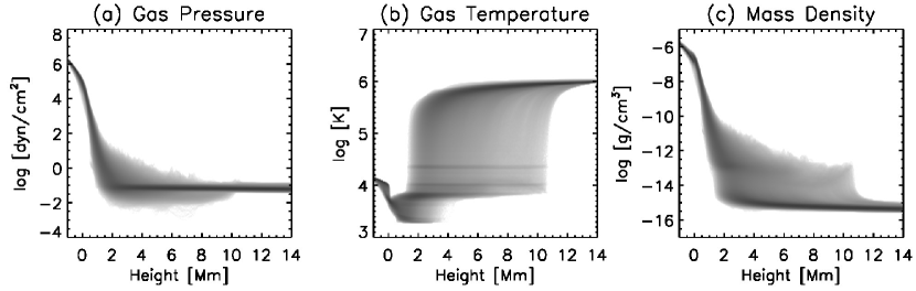
Figure 1: Vertical structure of the simulated atmosphere. The probability density functions (PDFs) of (a) gas pressure, (b) gas temperature, and (c) mass density are shown.

The stratification of the simulated plasma shows the vertically elongated chromosphere. Figure 1 shows the vertical structure of the simulated atmosphere. Because of the thermal conductive flux imposed at the top boundary, the coronal temperature is maintained at approximately 1 MK. The gas pressure and mass density are also uniform in the corona. We also observe that the cool chromospheric plasma with a mass density of $10^{-12}$–$10^{-14}$ g/cm³ covers the height range of 2–10 Mm. The result implies the existence of tall chromospheric jets in the simulation as shown in the following sections.

3.1 Morphology

Figure 2: Height of the chromosphere-corona transition region, which is defined as the height at which $T=$ 40000 K. Jet-A is located at $(X,Y)\sim(3,8)$ Mm. The variables of $Y>9$ Mm are calculated by assuming a periodic horizontal boundary condition.

The spatial structure of the tops of chromospheric jets can be visualized by the geometrical height of the transition region from the photospheric level. Figure 2 shows the time evolution of the height of the chromosphere-corona transition region. In this paper, we define the transition region as the height at which the temperature is equal to 40000 K. We find a tall jet that exceeds the maximum height of 10 Mm at time $=409.0$ min near $(X,Y)\sim(3,8)$ Mm. Hereafter, we call this tall jet Jet-A.

We also identify the fine-scale horizontal structures of chromospheric jets in Figure 2. Jet-A is a cluster of the fine-scale internal structures. The internal structure gradually becomes complex owing to the turbulent horizontal motion caused by the counter-clockwise rotation of Jet-A. This torsional motion is described in the next section.

The cluster of the fine-scale structures (Jet-A) gradually widens horizontally during the evolution (Figure 2). Jet-A initially has a horizontal diameter of approximately 2 Mm at time $=407.0$ min. The diameter reaches almost 4 Mm at time $=410.0$ min. The spatial deviation among the internal fine-scale structures increases during the evolution of the jet.

In this study, we focus on the properties and formation of Jet-A as a representative chromospheric jet in our simulation. Jet-A is the tallest chromospheric jet within the 30 min duration of the simulation. We find several jets exceeding the height of 7 Mm during the whole simulation run, with similar rotating motions and fine-scale structures.

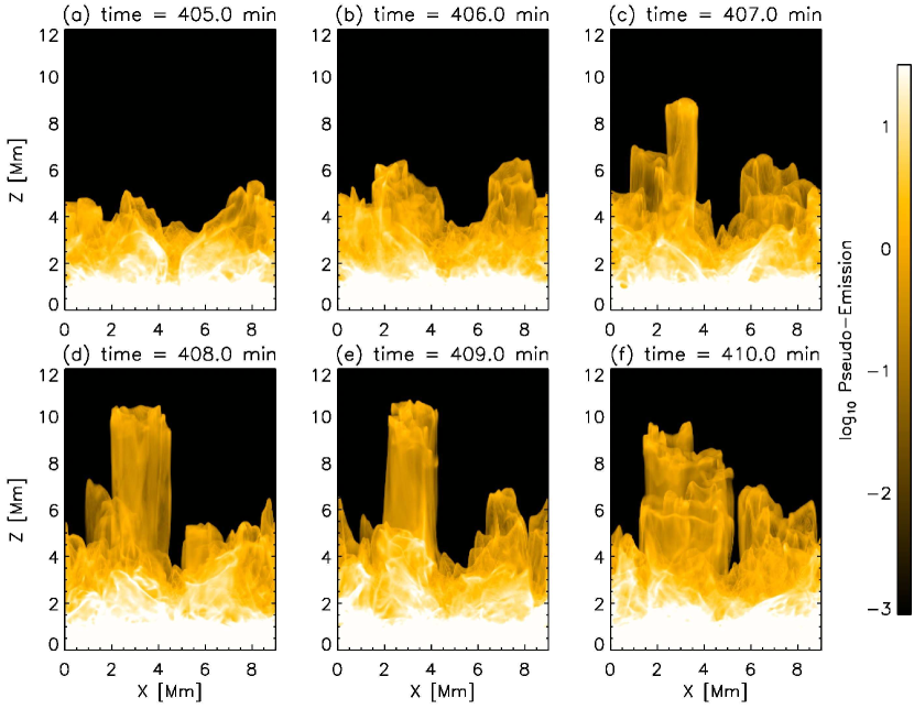
Figure 3: Six snapshots of the pseudo-emission defined in Eq. (5) and observed from the negative $Y$-direction. Jet-A is located at $X\sim 3$ Mm.

For the visualization mimicking the observation at the solar limb, we use pseudo-emission $\epsilon$ in the optically thin approximation defined as

$$\epsilon=\int n_{\mathrm{e}}n_{\mathrm{H}}G(T)\mathrm{d}l,$$ (5)

where $n_{\mathrm{e}}$ is the number density of electrons and $n_{\mathrm{H}}$ is the number density of hydrogen nuclei. The line integral is taken along the line-of-sight of the pseudo-observation. We assume a Gaussian form of the contribution function $G(T)$, given as

$$G(T)=C_{0}\exp\left[-\left(\frac{\log_{10}(T/T_{c})}{\varDelta\log_{10}T}\right)^{2}\right],$$ (6)

where we set $\log_{10}T_{c}\ \mathrm{[K]}=4.2$ and $\varDelta\log_{10}T=0.15$. The normalization constant $C_{0}=10^{-28}$ cm⁵ is taken such that the pseudo-emission in Eq. (5) becomes unity (dimensionless) for a plasma with a number density of $n_{\mathrm{e}}=n_{\mathrm{H}}=10^{10}$ cm^-3 and a line-of-sight thickness of 1 Mm. This contribution function is sensitive to the temperature range of the upper chromosphere.

The pseudo-emission from the negative $Y$-direction (Figure 3) shows the possible appearance of Jet-A when we observed at the solar limb. The line integral in Eq. (5) is taken over the whole $Y$-direction for each $(X,Z)$. Jet-A is located at $X\sim 3$ Mm. The top of the jet reaches a maximum height of approximately 10 Mm at time $=409.0$ min (Figure 3(e)). We also find finer jetting strands with a horizontal size of several hundreds of kilometers in Jet-A. The maximum height of $\approx 10$ Mm and the existence of the fine-scale structure are consistent with the findings in Figure 2.

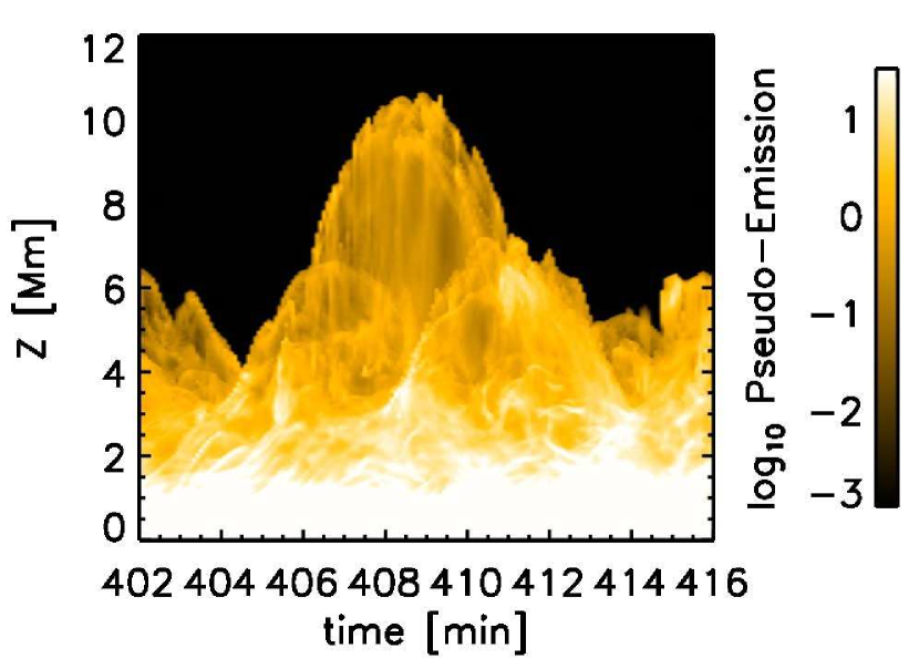
Figure 4: Time evolution of the pseudo-emission at the slit of $X=2.7$ Mm in Figure 3.

We put a vertical slit at $X=2.7$ Mm in Figure 3 for a more quantitative description of the vertical motion of Jet-A. Figure 4 shows the time evolution of the pseudo-emission of Jet-A. The top of Jet-A exhibits a nearly parabolic trajectory. The jet has a maximum elevation height of $\sim 7$ Mm and a lifetime of $\sim 9$ min. We estimate the maximum upward velocity of $\sim 50$ km/s and deceleration of $\sim 200$ m/s² by assuming a purely parabolic trajectory.

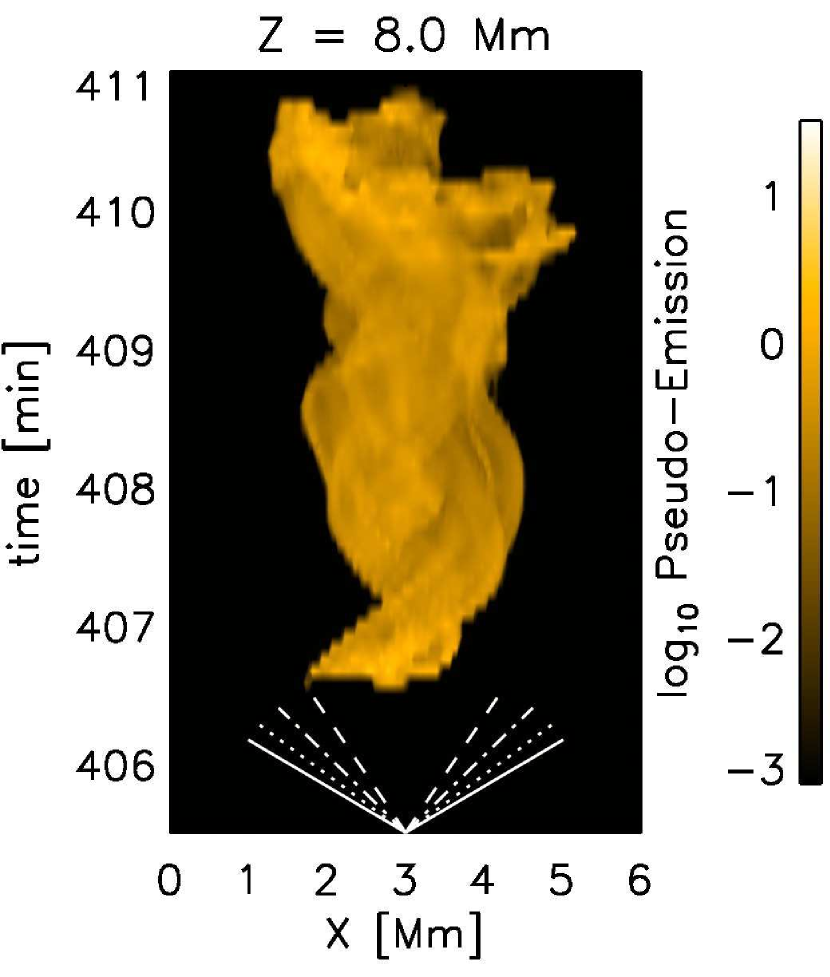
Figure 5: Time evolution of the horizontal slices of the pseudo-emission at the slit of $Z=8$ Mm in Figure 3. The white lines in each plot indicate the constant-velocities of 20 km/s (dashed), 30 km/s (dash-dotted), 40 km/s (dotted), and 50 km/s (solid) along the $X$-direction.

The pseudo-emission (Figure 3) also clarifies the apparent horizontal motion of the fine-scale strands in Jet-A. We put a horizontal slit at $Z=8$ Mm for a detailed description of the horizontal motion (Figure 5). We find wave-like patterns with apparent velocities of 30–40 km/s, displacements of $\approx 1$ Mm, and periods of 2–3 min. These patterns correspond to the horizontal displacement of fine-scale strands that follows the rotating motion of Jet-A which can be found in Figure 2.

When we interpret Jet-A as a single jet neglecting the internal structure, the apparent horizontal size of Jet-A changes in time within a period of several minutes (Figure 3). This temporal change in horizontal width is caused by the combination of the rotating motion of Jet-A and the temporal change of its internal horizontal structure, as shown in Figure 2. The apparent horizontal size of Jet-A gradually increases with the oscillation, probably owing to the centrifugal force of the rotation, as discussed in Section 4. Jet-A as a single jet also exhibits an apparent swaying motion. The horizontal velocity ($\approx 20$ km/s) and the displacement of the center ($\approx 0.5$ Mm) of this large-scale swaying pattern are slightly smaller than those of each strand because of the average effect.

3.2 Structure of Velocity and Magnetic Field

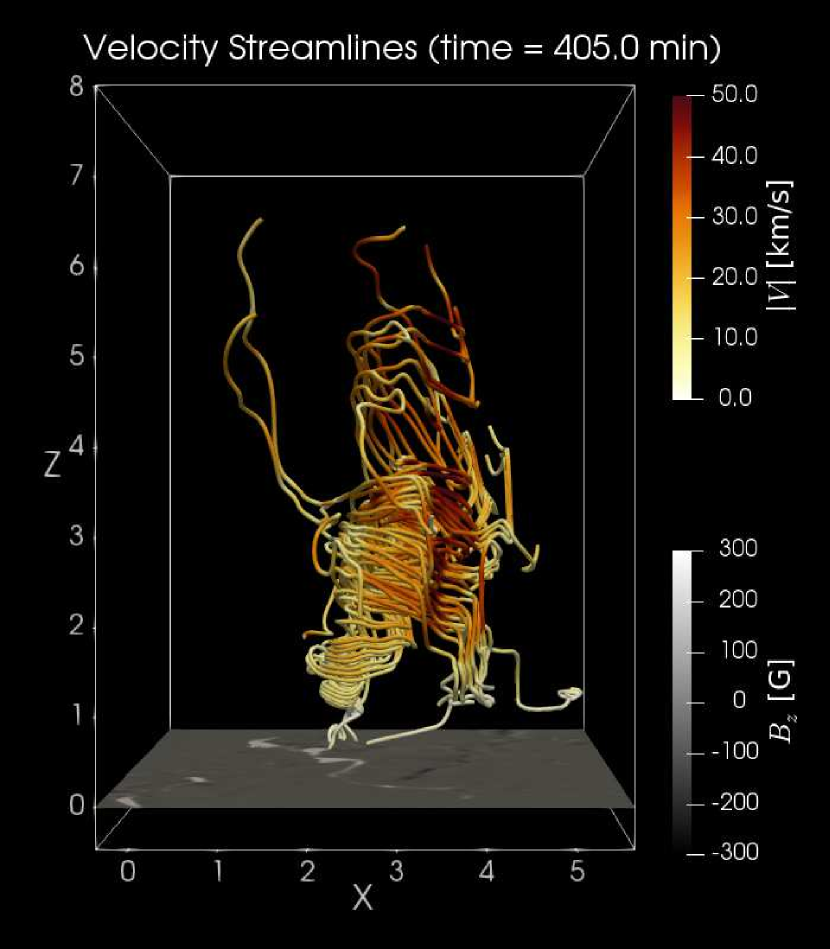
Figure 6: Three-dimensional structure of the velocity streamlines in a small box of $6\times 6\times 8.5$ Mm (including 0.5 Mm below $Z=0$ Mm) near the foot point of Jet-A located at $(X,Y)\sim(3,8)$ Mm. A snapshot at time of 405 min is shown. The horizontal slice of the vertical magnetic field at $Z=0$ Mm is also shown in gray scale. The color along the streamlines represents the magnitude of the velocity. (An animation of this figure is also available.)

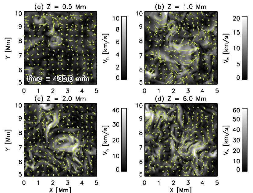
Figure 7: Horizontal slices of the absolute of the horizontal velocity at time $=$ 405.0 min. The horizontal slices are located at 0.5 Mm (panel (a)), 1.0 Mm (panel (b)), 2.0 Mm (panel (c)), and 6.0 Mm (panel (d)). The arrows in the right panels indicate the horizontal velocity field. The variables of $Y>9$ Mm are calculated by assuming a periodic horizontal boundary condition.

Near the root of Jet-A, an anticlockwise vertical vortex is found in the chromosphere (Figures 6 and 7). This strong vortex extends from the photosphere to the corona. The vortex is located at $(X,Y)\sim(2,8)$ near the temperature minimum (Figures 7(a)). The center of the vortex moves toward the positive $X$-direction and negative $Y$-direction in the higher layers (Figures 7(b)–(d)). The result indicates the inclination of the vertical vortex from the vertical axis. The strength of this chromospheric vortex is about 10–40 km/s depending on the measured height (Figures 7(b) and (c)). The vortex becomes wider in the higher region.

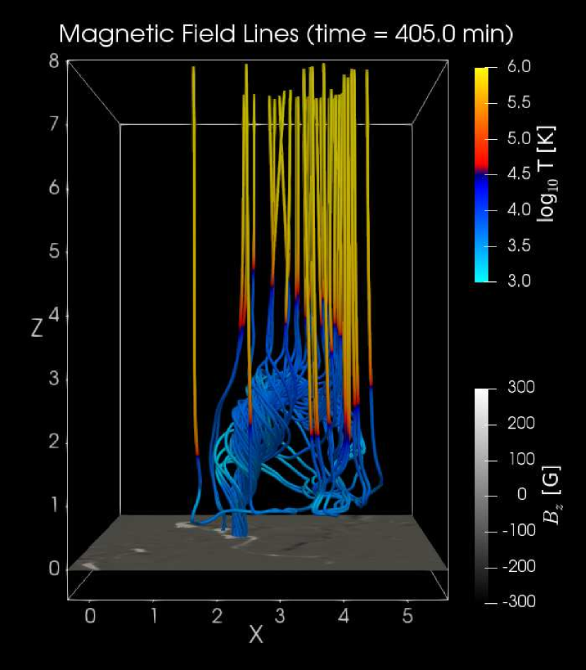
Figure 8: Same as Figure 6, but showing the three-dimensional structure of the magnetic field lines. The color along the magnetic field lines indicates the gas temperature. (An animation of this figure is also available.)

The magnetic field lines near the foot point of Jet-A are highly twisted in the chromosphere (Figure 8). We also find that the magnetic field lines are deformed near $(X,Z)\sim(4,1)$. The axis of the twist is inclined from the vertical axis as observed in the vortex structure (Figures 6 and 7). This result is interesting because the previous reports of the twisted magnetic field lines are relatively rare, although the torsional motion in the chromosphere has sometimes been reported in the simulations and observations (Wedemeyer-Böhm et al., 2012; Kitiashvili et al., 2013; Shelyag et al., 2013). A more detailed discussion on the comparison with the previous studies is given in Section 4.

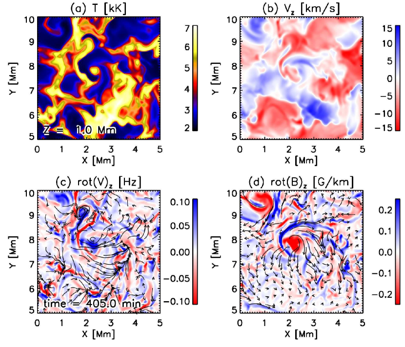
Figure 9: (a) Temperature, (b) vertical component of the velocity field, (c) vertical component of the vorticity, and (d) vertical component of the rotation of the magnetic field in the horizontal plane at $Z=1$ Mm and time $=$ 405.0 min. The arrows in panels (c) and (d) indicate the horizontal velocity and magnetic fields, respectively. The variables of $Y>9$ Mm are calculated by assuming a periodic horizontal boundary condition.

The twist of the magnetic field lines in the chromosphere is caused by the vortex motion. Figure 9 shows the horizontal slice at $Z=1$ Mm at the foot point of Jet-A. The small-scale swirl is found at $(X,Y)\sim(2,8)$ Mm. The lifetime of this swirl event is longer than 5 min. The swirl has a hot center with a downward flow and a cool edge with an upward flow. The vertical vorticity has a sign opposite to that of the vertical component of the curl of the magnetic field vector (Figures 9(c) and (d)), which is consistent with the upward-propagating torsional Alfvén wave. This result indicates that this swirl motion causes the twisted structure of the magnetic field lines in Figure 8.

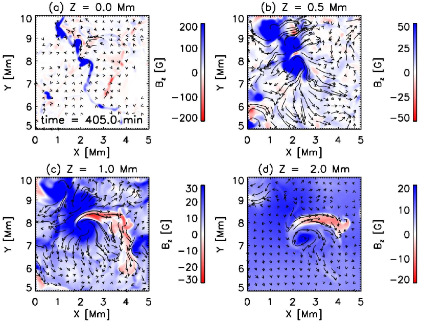
Figure 10: Vertical magnetic field at the four different layers of $Z=$ (a) 0.0, (b) 0.5, (c) 1.0, and (d) 2.0 Mm at time $=$ 405.0 min. Arrows indicate the horizontal component of the magnetic field. The variables of $Y>9$ Mm are calculated by assuming a periodic horizontal boundary condition.

We find a negative patch of the vertical magnetic field near the foot point of Jet-A in the middle of the chromosphere. Figure 10 shows the vertical magnetic field at various heights. The magnetic field lines through Jet-A originate from the photospheric magnetic flux concentration located at $(X,Y)\sim(2,8)$ Mm in Figure 10(a). We find a vertical magnetic field with the opposite polarity, which is located with a finite offset against the axis of the swirling motion in Figure 9. This opposite-polarity patch in the chromosphere (at $Z=$ 1.0 and 2.0 Mm; Figures 10(c) and 10(d), respectively) exists neither near the temperature minimum (at $Z=$ 0.5 Mm; Figure 10(b)) nor at the photospheric surface (at $Z=$ 0.0 Mm; Figure 10(a)). The direction of the horizontal magnetic field in this negative magnetic patch is the same as the nearby positive patch (Figures 10(c) and 10(d)).

Figure 11: Three-dimensional structure of the magnetic field lines. The horizontal slice of the vertical magnetic field at $Z=1$ Mm is shown in gray scale. Gas temperature on the $(Y,Z)$-plane at $X=2.5$ Mm is also shown. (An animation of this figure is also available.)

The negative magnetic patch in the chromosphere (Figure 10(c)) is a deformed part of the field lines connected to the positive patch in the photosphere. Figure 11 shows the three-dimensional topology of the magnetic field lines with the superposed horizontal slice at $Z=1$ Mm. The negative-polarity magnetic patch found in Figures 10(c) and (d) is a part of the positive magnetic patch located at $(X,Y,Z)\sim(2,8,0)$ Mm in Figure 10(a).

The torsional rotation near the foot point of Jet-A, which inclines slightly from the vertical axis, helps in producing these deformed magnetic field lines. The swirling magnetic field lines drag the heavy and cool plasma upward in the chromosphere (Figure 11). This dragged heavy plasma deforms the magnetic field lines and produces a negative magnetic patch in the middle chromosphere. These deformed magnetic field lines and the corresponding dragging motion also contribute to driving Jet-A, as will be discussed in Section 3.3.

3.3 Driving Mechanism of Chromospheric Jets

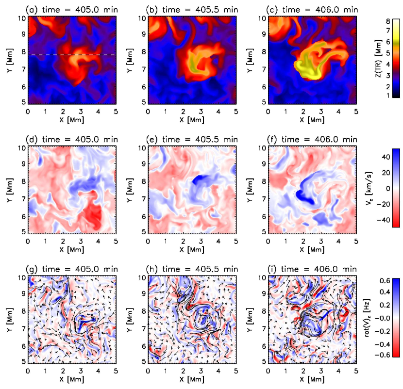
Figure 12: Time evolution of the transition region height (top row), vertical velocity (middle row), and vertical vorticity (middle row) at the transition region. Snapshots at time $=$ 405.0 (left column), 405.5 (middle column), and 406.0 min (right column) are shown. The horizontal dashed line in the top left panel represents the position of the slit ($Y=7.8$ Mm) plotted in Figures 13, 14, and 15. The arrows in the bottom panels indicate the horizontal velocity field at the transition region. The variables of $Y>9$ Mm are calculated by assuming a periodic horizontal boundary condition.

At time $=$ 405.0 min, Jet-A starts to rise exhibiting the anticlockwise rotation. Figure 12 shows a closed-up view of the initial emerging phase of Jet-A. The chromospheric jets begin to rise in the region of $X=$ 2–4 Mm and $Y\sim$ 8 Mm at time $=$ 405.0 min (Figures 12(a) and (d)), showing the anticlockwise rotation (Figure 12(g)). This initial rising region corresponds to the negative magnetic patch region in the chromosphere, as shown in Figures 10(c) and (d). The region continues to rise with the rotating motion following the the chromospheric vortex throughout the emergence of the chromospheric jet. The horizontal velocity increases the complexity during the emergence of Jet-A (Figure 10(i)), and produces the fine-scale structure of Jet-A.

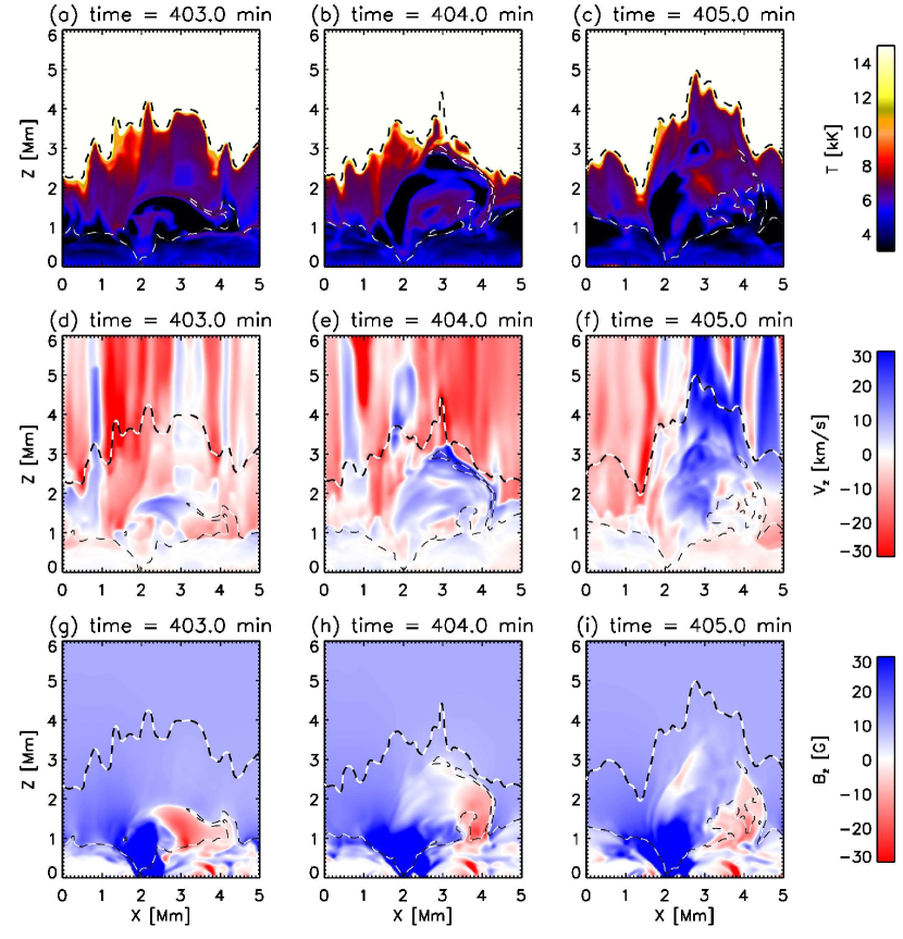
Figure 13: Time evolution on the $(X,Z)$-plane at $Y=7.8$ Mm. Shown are (a–c) the gas temperature, (d–f) vertical velocity, and (g–i) vertical magnetic field. The thin dashed lines indicate the plasma-beta unity. The thick dashed lines represent the position of the transition region, defined as the height at which the gas temperature becomes 40000 K.

Figure 14: Vertical slice on the $(X,Z)$-plane of $Y=7.8$ Mm at time $=403.0$ min. Shown are (a) the divergence of the velocity field, (b) the gas pressure, (c) the mass density, and (d) the magnetic pressure.

Before the top of Jet-A (i.e., the transition region) starts to rise, we identify the upward motion of a plasma blob in the chromosphere, with the shock front at the top, in the chromosphere. Figures 13 and 14 illustrate the time evolution of the chromospheric plasma in the driving process of Jet-A. The vertical slice of Figure 13 is located at the initial rising region of Jet-A (the dashed line in Figure 12(a)). At time $=403.0$ min, the cool plasma blob gradually moves upward with a vertical velocity of $\sim$ 10 km/s (Figures 13(a) and (d)). The shock front is formed at the top of this plasma blob as identified by the region with a strong velocity convergence (Figure 14(a)). Near the shock front, the gas pressure is enhanced by compression (Figure 14(b)).

The region inside the plasma blob is evacuated (i.e., low gas pressure) and highly magnetized. Below the shock front, the plasma blob has a lower gas pressure than the surroundings (Figure 14(b)). This reduction of the gas pressure is caused not by the reduction of mass density but by that of the gas temperature (Figures 13(a) and 14(c)) The magnetic field strength in this evacuated region is higher than that in the surrounding region (Figure 14(d)). This enhancement of the magnetic pressure corresponds to the negative magnetic patch in the chromosphere (Figures 10(c) and (d)) caused by the twisted and deformed magnetic field (Figures 8 and 11). This result implies that the contribution of the Lorentz force contributes to the formation process of Jet-A.

The cool and dense plasma blob hits the transition region and drives the tall chromospheric jet (Jet-A). The top of the upward-moving chromospheric plasma reaches the transition region at time $=404.0$ min (Figures 13(b), (e), and (h)). The amplitude of the upward velocity exceeds 30 km/s during the vertical propagation. At time $=405.0$ min (Figures 13(c), (f), and (i)), the shock front hits the transition region. The upward velocity is further amplified owing to the shock-transition region interaction (Hollweg, 1982). The chromospheric plasma continues to rise after the interaction and forms Jet-A. The region of the negative vertical magnetic field located at $X\sim$ 3–4 Mm is gradually diffused by the release of the twist of the magnetic field during the emergence of the chromospheric jet.

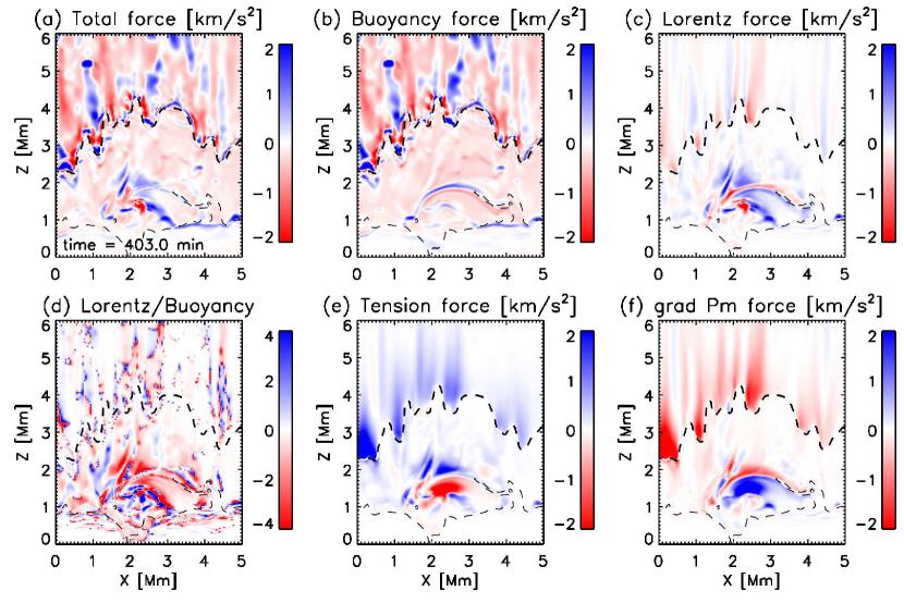
Figure 15: Same as Figure 14 but showing the vertical components of the driving forces. Shown are (a) the sum of the Lorentz force and the buoyancy force $F_{\mathrm{L}}+F_{\mathrm{B}}$, (b) the buoyancy (gas pressure gradient plus gravitational) force $F_{\mathrm{B}}$, (c) the Lorentz force $F_{\mathrm{L}}=F_{\mathrm{MP}}+F_{\mathrm{MT}}$, (d) the ratio between the Lorentz force and buoyancy forces $F_{\mathrm{L}}/F_{\mathrm{B}}$, (e) the magnetic pressure gradient force $F_{\mathrm{MP}}$, and (f) the magnetic tension force $F_{\mathrm{MT}}$. See the body text of this paper for the definitions of $F_{\mathrm{L}}$, $F_{\mathrm{B}}$, $F_{\mathrm{MP}}$, and $F_{\mathrm{MT}}$.

We evaluate the vertical component of the momentum equation to clarify the acceleration process of the cool plasma blob (shown in Figures 13 and 14) which drives Jet-A. The vertical components of the buoyancy force $F_{\mathrm{B}}$ and the Lorentz force $F_{\mathrm{L}}$ per unit mass are given by

$$F_{\mathrm{B}}=-\frac{1}{\rho}\frac{\partial P}{\partial z}+g_{z}$$ (7)

and

$$F_{\mathrm{L}}=\frac{1}{4\pi\rho}\left[\left(\nabla\times\bm{B}\right)\times\bm{B}\right]_{z},$$ (8)

respectively. We decompose the Lorentz force $F_{\mathrm{L}}$ into the magnetic pressure gradient force $F_{\mathrm{MP}}$ and the magnetic tension force $F_{\mathrm{MT}}$ for a clearer interpretation. These forces are written as

$$F_{\mathrm{MP}}=-\frac{1}{\rho}\frac{\partial P_{m}}{\partial z}+\frac{b_{z}}{\rho}\left(\bm{b}\cdot\nabla\right)P_{m}$$ (9)

and

$$F_{\mathrm{MT}}=F_{\mathrm{L}}-F_{\mathrm{MP}},$$ (10)

respectively, where $P_{m}=B^{2}/(8\pi)$ is the magnetic pressure and $\bm{b}=\bm{B}/B$ is the unit vector in the direction of the magnetic field.

We find that the upward motion of the cool plasma blob and the resulting chromospheric jet (Jet-A) is driven by the Lorentz force, especially by the magnetic pressure gradient force. Figure 15 shows the vertical slice of the driving forces. The buoyancy force mainly acts downward except near the shock front where the pressure gradient force acts both upward and downward (Figure 15(b)). The Lorentz force is relatively strong and mainly acts upward (15(c)). As shown in Figure 15(d), the Lorentz force is the dominant driver of the upward motion of the cool chromospheric plasma blob (Figures 13 and 14). In particular, the magnetic pressure gradient force $F_{\mathrm{MP}}$ acts upward at the plasma blob (Figure 15(e)). The magnetic tension force (Figure 15(f)) tends to compensate for the magnetic pressure gradient force. In total (Figure 15(a)), the left part of the cool plasma blob is accelerated upward by the magnetic pressure gradient force. From the above results, we conclude that the chromospheric shock wave, as an energy source of Jet-A, is driven by the magnetic pressure gradient force.

We will now summarize the formation process of the tallest chromospheric jet in our simulation (Jet-A):

1. First, the twisted magnetic field structure is generated by the vortex motion at the root of the jet (Figure 8). A part of the magnetic field lines is dragged and deformed by the lower chromospheric plasma owing to the inclination of the vortex away from the vertical axis (Figure 7).

2. After a sufficiently large magnetic twist is stored, these deformed magnetic field lines start to lift up the dense and cool chromospheric plasma to the upper layer by the Lorentz force (Figures 11 and 15).

3. The accelerated chromospheric plasma exceeds the sound speed and becomes a shock wave (Figure 14). The shock wave hits the transition region and finally forms the chromospheric jet (Figure 13).

4 Discussion

We briefly compare our simulation with the observed chromospheric jets. In this paper, we present the results of a three-dimensional simulation of solar chromospheric jets. We successfully reproduce a chromospheric jet (Jet-A) with a maximum height of 10–11 Mm and lifetime of 8–10 min. The tall chromospheric jet in our simulation shows a parabolic path with a maximum velocity of approximately 50 km/s, and a deceleration of approximately 200 m/s². These parameters are in good agreement with the observed properties of the spicules (or more precisely the classical Type I spicules) in quiet regions (Skogsrud et al., 2015). These jets emanate from a strong magnetic flux tube below and are driven by a Lorentz force related to the rotational motion of the flux tube.

The driving mechanism and resulting jet in our simulation are similar to those in the one-dimensional Alfvén wave models of chromospheric jets presented in the previous studies, but they also exhibit several differences. The chromospheric jet described in this paper originates from the vortex motion in the lower atmosphere. In this sense, our model is categorized as a family of the Alfvén wave models of spicules (Hollweg et al., 1982; Kudoh & Shibata, 1999). However, there are several differences from previous studies concerning the driving mechanism and resulting jets caused by the axial asymmetry of the vortex in the three-dimensional domain.

One such differences from the one-dimensional models is that the inclination of the vortex tube also plays a role in the driving process of our simulation. We show that the inclined rotation of the magnetic field lines lifts the dense chromospheric plasma upward. In one-dimensional the Alfvén wave models, the nonlinearity or amplitude of the Alfvén wave is important for the generation of chromospheric jets, since the highly nonlinear Alfvén wave is required to produce the acoustic wave (or shock wave) through the mode conversion (Hollweg, 1971). We suggest that the inclination of the magnetic flux tube may also helps in increasing the twist of the magnetic field (and the nonlinearity of the Alfvén wave) in the chromosphere.

Another large difference between our study and one-dimensional axisymmetric Alfvén wave models is that the chromospheric jet has a fine-scale axially asymmetric structure. The produced chromospheric jet forms a cluster with a diameter of several Mm that consists of the finer strands as shown in Figures 2 and 3. This result is consistent with the multi-threaded nature of spicules (Suematsu et al., 2008; Sterling et al., 2010; Skogsrud et al., 2014). We also find that the horizontal size of the cluster of strands gradually becomes wider during the evolution of the jet. This is probably related to the centrifugal force of the rotation of the jet. The rotation of the whole cluster with the independent separating motion of finer strands found in our simulation reminds us of the separation and connection of the spicule strands and the spatial broadening and diffusion of spicules (Sterling et al., 2010). Skogsrud et al. (2014) suggested that the Kelvin-Helmholtz instability caused by the swaying motion produces this multi-threaded nature as in the coronal loop simulations (Antolin et al., 2014). The difference is that our chromospheric jets are driven by rotational rather than swaying motion. Suematsu et al. (2008) interpreted the separation of threads by assuming the torsional motion of a spicule as a rigid body. Although their interpretation also works in our model, our horizontal structure seems to be closely related to the jet’s formation process. It is not easy to determine the main contributor of the fine-scale horizontal structure formation from the several candidates such as the horizontal inhomogeneity of the initial driver or latter Kelvin-Helmholtz instability. We also note that our pseudo-emission, shown in Figure 3, is not the real radiative emission observed in the solar chromosphere. Under the limitations described above, our current interpretation of the formation process of the horizontal structure in Jet-A is as follows:

1. Initially, the large-scale (anticlockwise) rotation with a typical diameter of 0.5–1.0 Mm is driven by the release of the magnetic twist in the chromosphere (Figure 7).

2. During the evolution, the strong velocity shear between Jet-A and the surrounding coronal plasma causes the Kelvin-Helmholtz instability and forms a multi-strand structure with smaller vortices with a typical diameter smaller than several hundreds of kilometers. The small-scale clockwise rotation (Figures 12) is generated in this stage. The initially small phase difference of the Alfvén wave will be also enhanced, helping in forming the fine-scale structure.

3. Resulting fine-scale strands are separated by the centrifugal force of the initial large-scale anticlockwise rotation (Figures 2 and 3).

Further analysis is required to clarify the exact mechanism of horizontal structure formation and the relationship between the radiative emission and the horizontal structure of the chromospheric plasma.

We have shown that the simulated chromospheric jet exhibits the apparent horizontal oscillation during its lifetime (Figure 5). The period of several minutes and the amplitude of 20-30 km/s are consistent with the observational oscillatory nature of solar spicules (Zaqarashvili & Erdélyi, 2009). In our model, the initial anticlockwise torsional motion and the small-scale vortices of the fine-scale strands are the origin of this apparent oscillation. It should be noted that the apparent periodicity of (pseudo-)radiative emission does not indicate the periodic motion of the actual plasma motion. The combination of the fine-scale structure inside the jet and the vortex is the origin of the apparent periodicity or oscillation. One important aspect of our model is that the density and horizontal velocity structure are not axisymmetric. This reveals the importance of considering the non-axisymmetric model to understand the oscillation of observed spicules. Since we use a very rough approximation to compute the (pseudo-)radiative emission, a more detailed analysis should be carried out to compare Jet-A with the observation. The propagation of the produced oscillation should also be investigated in the future.

We find a strong vortex at the root of the tall chromospheric jet. The tornado-like streamlines above the strong magnetic concentration have been reported by Wedemeyer-Böhm et al. (2012) and numerically investigated by several authors (Wedemeyer-Böhm et al., 2012; Kitiashvili et al., 2013; Shelyag et al., 2013; Wedemeyer & Steiner, 2014; Kato & Wedemeyer, 2017) without including the corona above the chromosphere. In our simulation, the chromospheric magnetic field is also twisted following the swirling motion. Kitiashvili et al. (2013) reported weakly twisted magnetic field lines produced by chromospheric swirls with an average vertical magnetic field strength of 10 G, which is exactly the same as that in our case. A hot center with a downward flow and a cool edge with an upward flow of their swirl event are also found in both their swirl and our simulation. The existence of chromospheric jets and the highly twisted magnetic field lines is probably produced by the inclusion of the corona above the chromosphere. The simulations conducted by Wedemeyer-Böhm et al. (2012) and Shelyag et al. (2013) investigated the cases with a stronger magnetic field. Both of studies exhibited little twist of the magnetic field probably owing to the high Alfvén speed in the chromosphere. The effect of the average vertical magnetic field strength on the formation of chromospheric jets should be investigated in the future.

One of the limitations of our model is the spatial grid size of the simulation. We find that, in the two-dimensional simulation (Iijima & Yokoyama, 2015), the width or the horizontal size of the jets becomes finer when a smaller grid size is used. Similar phenomena can occur in our model. The rotational motion driven in the photosphere and the upper convection zone also require spatial resolution because the magnetic field is intensified into small flux tubes in the photosphere. Note that our simulation does not produce tall jets such as reported in this study if we double the horizontal grid size (low spatial resolution) used for the simulation.

Another limitation of our model is the approximations in the equations of state and the radiative cooling. The LTE equation of states and simplified radiative cooling are used in this study. The large amplitude of radiative cooling reduces the length and maximum velocity of the produced chromospheric jets by damping the chromospheric acoustic/shock waves (Sterling & Mariska, 1990; Guerreiro et al., 2013). The assumption of the LTE equation of states in the chromosphere causes an error in the heat capacity (or gas temperature) and the electron number density. The effect of non-equilibrium ionization (Carlsson & Stein, 2002; Leenaarts & Wedemeyer-Böhm, 2006; Leenaarts et al., 2007; Wedemeyer-Böhm & Carlsson, 2011; Golding et al., 2014, 2016) on the formation of chromospheric jets should be investigated in the future.

The effect of the collisions between the ions and neutrals is another issue to be studied. This effect appears in the Ohm’s law as additional terms in the one-fluid MHD equations. In our calculations here, no explicit resistivity besides the numerical diffusivity is introduced. The importance of the Hall effect or the ambipolar diffusion in the solar chromosphere is suggested by the previous studies (e.g., Martínez-Sykora et al., 2012; Cheung & Cameron, 2012; Leake et al., 2014; Martínez-Sykora et al., 2015; Khomenko, 2017) More recently, Martínez-Sykora et al. (2017) have suggested that the ambipolar diffusion helps in increasing the length of chromospheric jets driven by the tension force. As we have shown, the dragging of the chromospheric plasma by the torsional motion plays an important role in the production of chromospheric jets. In the real solar chromosphere, the ambipolar diffusion produced by the drift motion between the ions and neutrals will reduce the dragging efficiency of the chromospheric plasma, leading to shorter chromospheric jets. A similar reduction in the chromospheric plasma drag has been investigated in the context of flux emergence and active region formation (Leake & Arber, 2006; Arber et al., 2007; Leake & Linton, 2013). Another effect of the ambipolar diffusion is its assistance in the formation of thin current sheets (Parker, 1963; Brandenburg & Zweibel, 1994) and the occurrence of fast magnetic reconnection in the chromosphere. It should also be noted that, because the amount of the ambipolar diffusion strongly depends on the ionization rate, the detailed treatment of the equation of state (Leenaarts et al., 2007; Golding et al., 2016) or the amount of the radiative cooling (Laguna et al., 2017) will cause significant differences on the simulation results. Further work with a greater focus on the ambipolar diffusion should be undertaken.

We find a chromospheric jet that is significantly taller than those in similar three-dimensional radiative MHD simulations (Martínez-Sykora et al., 2009, 2011; Hansteen et al., 2015). These simulations employed the Oslo Stagger code or the Bifrost code (Gudiksen et al., 2011) with a more realistic treatment of the radiation. Because of the many differences between our code (RAMENS) and Bifrost, it is not easy to understand what causes this difference. One candidate is the assumption of closed loop configuration for the magnetic field in their study. This possibly acts to reduce the maximum height of the chromospheric jets that extend along the loop. The closed loop also acts to heat the corona more easily. This prevents the nonlinear amplification of the chromospheric shock wave (Shibata & Suematsu, 1982; Iijima & Yokoyama, 2015), leading to shorter jets. The numerical dissipation of the MHD scheme is also important. As discussed above, we do not find tall chromospheric jets, like Jet-A, at a lower spatial resolution. Hansteen et al. (2015) obtained results with different grid sizes and showed that the chromospheric material is more elongated for a finer spatial grid. The treatment of the radiative cooling is also a possible cause of the difference. Stronger radiative cooling causes stronger damping of the chromospheric shock waves. Therefore, the resulting chromospheric jets will be shorter. A more detailed comparison is required to show the dominant source of difference between our results and those of previous studies.

5 Conclusion

We have presented a radiation magnetohydrodynamic simulation of chromospheric jets. A tall chromospheric jet (Jet-A) is reproduced by the Lorentz force of the twisted magnetic field lines. Jet-A also exhibits horizontal oscillatory motion and fine-scale internal structure during its emergence. Our model is a three-dimensional extension of the classical Alfvén wave model of chromospheric jets. In this study, the most significant characteristic of the model is that the all of the driving mechanism, multi-strand structure, and oscillatory nature are closely related to each other and explained in a model. We conclude that the Alfvén wave model, or the torsional wave model of spicules, is an important candidate for explaining the driving mechanism of solar spicules.

References

- Antolin et al. (2014) Antolin, P., Yokoyama, T., & Van Doorsselaere, T. 2014, ApJ, 787, L22
- Arber et al. (2007) Arber, T. D., Haynes, M., & Leake, J. E. 2007, ApJ, 666, 541
- Asplund et al. (2006) Asplund, M., Grevesse, N., & Sauval, A. J. 2006, Communications in Asteroseismology, 147, 76
- Beck et al. (2016) Beck, C., Rezaei, R., Puschmann, K. G., & Fabbian, D. 2016, Sol. Phys., 291, 2281
- Beckers (1963) Beckers, J. M. 1963, ApJ, 138, 648
- Beckers (1968) —. 1968, Sol. Phys., 3, 367
- Beckers (1972) —. 1972, ARA&A, 10, 73
- Brandenburg & Zweibel (1994) Brandenburg, A., & Zweibel, E. G. 1994, ApJ, 427, L91
- Carlsson & Stein (2002) Carlsson, M., & Stein, R. F. 2002, ApJ, 572, 626
- Cheung & Cameron (2012) Cheung, M. C. M., & Cameron, R. H. 2012, ApJ, 750, 6
- De Pontieu et al. (2012) De Pontieu, B., Carlsson, M., Rouppe van der Voort, L. H. M., et al. 2012, ApJ, 752, L12
- De Pontieu & Haerendel (1998) De Pontieu, B., & Haerendel, G. 1998, A&A, 338, 729
- De Pontieu et al. (2007a) De Pontieu, B., Hansteen, V. H., Rouppe van der Voort, L., van Noort, M., & Carlsson, M. 2007a, ApJ, 655, 624
- De Pontieu et al. (2007b) De Pontieu, B., McIntosh, S., Hansteen, V. H., et al. 2007b, PASJ, 59, 655
- De Pontieu et al. (2007c) De Pontieu, B., McIntosh, S. W., Carlsson, M., et al. 2007c, Science, 318, 1574
- Erdélyi & Fedun (2007) Erdélyi, R., & Fedun, V. 2007, Science, 318, 1572
- Golding et al. (2014) Golding, T. P., Carlsson, M., & Leenaarts, J. 2014, ApJ, 784, 30
- Golding et al. (2016) Golding, T. P., Leenaarts, J., & Carlsson, M. 2016, ApJ, 817, 125
- González-Avilés et al. (2017) González-Avilés, J. J., Guzmán, F. S., & Fedun, V. 2017, ApJ, 836, 24
- Gudiksen et al. (2011) Gudiksen, B. V., Carlsson, M., Hansteen, V. H., et al. 2011, A&A, 531, A154
- Guerreiro et al. (2013) Guerreiro, N., Carlsson, M., & Hansteen, V. 2013, ApJ, 766, 128
- Hansteen et al. (2015) Hansteen, V., Guerreiro, N., De Pontieu, B., & Carlsson, M. 2015, ApJ, 811, 106
- Hansteen et al. (2006) Hansteen, V. H., De Pontieu, B., Rouppe van der Voort, L., van Noort, M., & Carlsson, M. 2006, ApJ, 647, L73
- Heggland et al. (2009) Heggland, L., De Pontieu, B., & Hansteen, V. H. 2009, ApJ, 702, 1
- Heggland et al. (2011) Heggland, L., Hansteen, V. H., De Pontieu, B., & Carlsson, M. 2011, ApJ, 743, 142
- Hollweg (1971) Hollweg, J. V. 1971, J. Geophys. Res., 76, 5155
- Hollweg (1982) —. 1982, ApJ, 257, 345
- Hollweg et al. (1982) Hollweg, J. V., Jackson, S., & Galloway, D. 1982, Sol. Phys., 75, 35
- Iijima (2016) Iijima, H. 2016, PhD thesis, Department of Earth and Planetary Science, School of Science, The University of Tokyo, Japan, doi:10.5281/zenodo.55411
- Iijima & Yokoyama (2015) Iijima, H., & Yokoyama, T. 2015, ApJ, 812, L30
- James & Erdélyi (2002) James, S. P., & Erdélyi, R. 2002, A&A, 393, L11
- Kato et al. (2016) Kato, Y., Steiner, O., Hansteen, V., et al. 2016, ApJ, 827, 7
- Kato et al. (2011) Kato, Y., Steiner, O., Steffen, M., & Suematsu, Y. 2011, ApJ, 730, L24
- Kato & Wedemeyer (2017) Kato, Y., & Wedemeyer, S. 2017, A&A, 601, A135
- Khomenko (2017) Khomenko, E. 2017, Plasma Physics and Controlled Fusion, 59, 014038
- Kitiashvili et al. (2013) Kitiashvili, I. N., Kosovichev, A. G., Lele, S. K., Mansour, N. N., & Wray, A. A. 2013, ApJ, 770, 37
- Kudoh & Shibata (1999) Kudoh, T., & Shibata, K. 1999, ApJ, 514, 493
- Laguna et al. (2017) Laguna, A. A., Lani, A., Mansour, N., Deconinck, H., & Poedts, S. 2017, The Astrophysical Journal, 842, 16pp
- Leake & Arber (2006) Leake, J. E., & Arber, T. D. 2006, A&A, 450, 805
- Leake & Linton (2013) Leake, J. E., & Linton, M. G. 2013, ApJ, 764, 54
- Leake et al. (2014) Leake, J. E., DeVore, C. R., Thayer, J. P., et al. 2014, Space Sci. Rev., 184, 107
- Leenaarts et al. (2007) Leenaarts, J., Carlsson, M., Hansteen, V., & Rutten, R. J. 2007, A&A, 473, 625
- Leenaarts & Wedemeyer-Böhm (2006) Leenaarts, J., & Wedemeyer-Böhm, S. 2006, A&A, 460, 301
- Martínez-Sykora et al. (2012) Martínez-Sykora, J., De Pontieu, B., & Hansteen, V. 2012, ApJ, 753, 161
- Martínez-Sykora et al. (2015) Martínez-Sykora, J., De Pontieu, B., Hansteen, V., & Carlsson, M. 2015, Philosophical Transactions of the Royal Society of London Series A, 373, 40268
- Martínez-Sykora et al. (2017) Martínez-Sykora, J., De Pontieu, B., Hansteen, V. H., et al. 2017, Science, 356, 1269
- Martínez-Sykora et al. (2009) Martínez-Sykora, J., Hansteen, V., De Pontieu, B., & Carlsson, M. 2009, ApJ, 701, 1569
- Martínez-Sykora et al. (2011) Martínez-Sykora, J., Hansteen, V., & Moreno-Insertis, F. 2011, ApJ, 736, 9
- Okamoto & De Pontieu (2011) Okamoto, T. J., & De Pontieu, B. 2011, ApJ, 736, L24
- Ôno et al. (1960) Ôno, Y., Sakashita, S., & Yamazaki, H. 1960, Progress of Theoretical Physics, 23, 294
- Osterbrock (1961) Osterbrock, D. E. 1961, ApJ, 134, 347
- Parker (1963) Parker, E. N. 1963, ApJS, 8, 177
- Parker (1964) —. 1964, ApJ, 140, 1170
- Pereira et al. (2014) Pereira, T. M. D., De Pontieu, B., Carlsson, M., et al. 2014, ApJ, 792, L15
- Pikel’ner (1969) Pikel’ner, S. B. 1969, Soviet Ast., 13, 259
- Pikel’ner (1971) —. 1971, Comments on Astrophysics and Space Physics, 3, 33
- Roberts (1945) Roberts, W. O. 1945, ApJ, 101, 136
- Secchi (1875) Secchi, A. 1875, Le Soleil, doi:10.3931/e-rara-14748
- Shelyag et al. (2013) Shelyag, S., Cally, P. S., Reid, A., & Mathioudakis, M. 2013, ApJ, 776, L4
- Shibata & Suematsu (1982) Shibata, K., & Suematsu, Y. 1982, Sol. Phys., 78, 333
- Singh et al. (2011) Singh, K. A. P., Shibata, K., Nishizuka, N., & Isobe, H. 2011, Physics of Plasmas, 18, 111210
- Skartlien et al. (2000) Skartlien, R., Stein, R. F., & Nordlund, Å. 2000, ApJ, 541, 468
- Skogsrud et al. (2014) Skogsrud, H., Rouppe van der Voort, L., & De Pontieu, B. 2014, ApJ, 795, L23
- Skogsrud et al. (2015) Skogsrud, H., Rouppe van der Voort, L., De Pontieu, B., & Pereira, T. M. D. 2015, ApJ, 806, 170
- Steiner et al. (1998) Steiner, O., Grossmann-Doerth, U., Knölker, M., & Schüssler, M. 1998, ApJ, 495, 468
- Sterling (2000) Sterling, A. C. 2000, Sol. Phys., 196, 79
- Sterling & Mariska (1990) Sterling, A. C., & Mariska, J. T. 1990, ApJ, 349, 647
- Sterling et al. (2010) Sterling, A. C., Moore, R. L., & DeForest, C. E. 2010, ApJ, 714, L1
- Suematsu et al. (2008) Suematsu, Y., Ichimoto, K., Katsukawa, Y., et al. 2008, in Astronomical Society of the Pacific Conference Series, Vol. 397, First Results From Hinode, ed. S. A. Matthews, J. M. Davis, & L. K. Harra, 27
- Suematsu et al. (1982) Suematsu, Y., Shibata, K., Neshikawa, T., & Kitai, R. 1982, Sol. Phys., 75, 99
- Takasao et al. (2013) Takasao, S., Isobe, H., & Shibata, K. 2013, PASJ, 65, 62
- Thomas (1948) Thomas, R. N. 1948, ApJ, 108, 130
- Tsiropoula et al. (2012) Tsiropoula, G., Tziotziou, K., Kontogiannis, I., et al. 2012, Space Sci. Rev., 169, 181
- Uchida (1961) Uchida, Y. 1961, PASJ, 13, 321
- Uchida (1969) —. 1969, PASJ, 21, 128
- Wedemeyer & Steiner (2014) Wedemeyer, S., & Steiner, O. 2014, PASJ, 66, S10
- Wedemeyer-Böhm & Carlsson (2011) Wedemeyer-Böhm, S., & Carlsson, M. 2011, A&A, 528, A1
- Wedemeyer-Böhm et al. (2012) Wedemeyer-Böhm, S., Scullion, E., Steiner, O., et al. 2012, Nature, 486, 505
- Zaqarashvili & Erdélyi (2009) Zaqarashvili, T. V., & Erdélyi, R. 2009, Space Sci. Rev., 149, 355
- Zhang et al. (2012) Zhang, Y. Z., Shibata, K., Wang, J. X., et al. 2012, ApJ, 750, 16