Balancing information exposure in social networks

Abstract

Social media has brought a revolution on how people are consuming news. Beyond the undoubtedly large number of advantages brought by social-media platforms, a point of criticism has been the creation of echo chambers and filter bubbles, caused by social homophily and algorithmic personalization.

In this paper we address the problem of balancing the information exposure in a social network. We assume that two opposing campaigns (or viewpoints) are present in the network, and that network nodes have different preferences towards these campaigns. Our goal is to find two sets of nodes to employ in the respective campaigns, so that the overall information exposure for the two campaigns is balanced. We formally define the problem, characterize its hardness, develop approximation algorithms, and present experimental evaluation results.

Our model is inspired by the literature on influence maximization, but we offer significant novelties. First, balance of information exposure is modeled by a symmetric difference function, which is neither monotone nor submodular, and thus, not amenable to existing approaches. Second, while previous papers consider a setting with selfish agents and provide bounds on best response strategies (i.e., move of the last player), we consider a setting with a centralized agent and provide bounds for a global objective function.

1 Introduction

Social-media platforms have revolutionized many aspects of human culture, among others, the way people are exposed to information. A recent survey estimates that 62% of adults in the US get their news on social media [20]. Despite providing many desirable features, such as, searching, personalization, and recommendations, one point of criticism is that social media amplify the phenomenon of echo chambers and filter bubbles: users get less exposure to conflicting viewpoints and are isolated in their own informational bubble. This phenomenon is contributed to social homophily and algorithmic personalization, and is more acute for controversial topics [2, 12, 13, 16, 18].

In this paper we address the problem of reducing the filter-bubble effect by balancing information exposure among users. We consider social-media discussions around a topic that are characterized by two or more conflicting viewpoints. Let us refer to these viewpoints as campaigns. Our approach follows the popular paradigm of influence propagation [24]: we want to select a small number of seed users for each campaign so as to maximize the number of users who are exposed to both campaigns. In contrast to existing work on competitive viral marketing, we do not consider the problem of finding an optimal selfish strategy for each campaign separately. Instead we consider a certalized agent responsible for balancing information exposure for the two campaings. Consider the following motivating examples.

Example 1: Prominent social-media companies, like Facebook and Twitter, have been called to act as arbiters so as to prevent ideological isolation and polarization in the society. The motivation for companies to assume this role could be for improving their public image or due to government policies. Consider a controversial topic being discussed in social-media platform $X$, which has led to polarization and filter bubbles. Platform $X$ has the ability to algorithmically detect such bubbles [16], identify the influential users on each side, and estimate the influence among users [14, 19]. As part of a new filter-bubble bursting service, platform $X$ would like to disseminate two high-quality and thought-provoking dueling op-eds, articles, one for each side, that present the arguments of the other side in a fair manner. Assume that $X$ is interested in following a viral-marketing approach. Which users should $X$ target, for each of the two articles, so that people in the network are informed in the most balanced way?

Example 2: Government organization $Y$ is initiating a programme to help assimilate foreigners who have newly arrived in the country. Part of the initiative focuses on bringing the communities of foreigners and locals closer in social media. Organization $Y$ is interested in identifying individuals who can help spreading news of one community into the other.

From the technical standpoint, we consider the following problem setting: We assume that information is propagated in the network according to the independent-cascade model [24]. We assume that there are two opposing campaigns, and for each one there is a set of initial seed nodes, $I_{1}$ and $I_{2}$, which are not necessarily distinct. Furthermore, we assume that the users in the network are exposed to information about campaign $i$ via diffusion from the set of seed nodes $I_{i}$. The diffusion in the network may occur with independent or correlated probabilities for the two campaigns; we consider both settings to which we are referring as heterogeneous or correlated.

The objective is to recruit two additional sets of seed nodes, $S_{1}$ and $S_{2}$, for the two campaigns, with ${\left|S_{1}\right|}+{\left|S_{2}\right|}\leq k$, for a given budget $k$, so as to maximize the expected number of balanced users, i.e., the users who are exposed to information from both campaigns (or from none!).

We formally define the problem of balancing information exposure and we show that it is $\mathbf{NP}$-hard. We develop different approximation algorithms for the different settings we consider, as well as heuristic variants of the proposed algorithm. We experimentally evaluate our methods, on several real-world (and realistic) datasets, collected from twitter, for different topics of interest.

Although our approach is inspired by the large body of work on information propagation, and resembles previous problem formulations for competitive viral marketing, there are significant differences and novelties. In particular:

• This is the first paper to address the problem of balancing information exposure and breaking filter bubbles, using the information-propagation methodology.

• The objective function that best suits our problem setting is related to the size of the symmetric difference of users exposed to the two campaigns. This is in contrast to previous settings that consider functions related to the size of the coverage of the campaigns.

• As a technical consequence of the previous point, our objective function is neither monotone nor submodular making our problem more challenging. Yet we are able to analyze the problem structure and provide algorithms with approximation guarantees.

• While most previous papers consider selfish agents, and provide bounds on best-response strategies (i.e., move of the last player), we consider a centralized setting and provide bounds for a global objective function.

We note that our datasets and implementation is publicly available.

2 Related Work

Detecting and breaking filter bubbles. Several studies have observed that users in online social networks prefer to associate with like-minded individuals and consume agreeable content. This phenomenon leads to filter bubbles, echo chambers [36, 35], and to online polarization [1, 2, 5, 12, 16, 22, 30]. Once these filter bubbles are detected, the next step is to try to overcome them. One way to achieve this is by making recommendations to individuals of opposing viewpoints. This idea has been explored, in different ways, by a number of studies in the literature [17, 26, 27, 31, 39]. However, all previous studies address the problem of breaking filter bubbles by the means of content recommendation. To the best of our knowledge, this is the first paper that considers an information diffusion approach.

Information diffusion. Following a large body of work, we model diffusion using the independent-cascade model [24]. In the basic model a single item propagates in the network. An extension is when multiple items propagate simultaneously. All works that study optimization problems in the case of multiple items, consider that items compete for being adopted by users. In other words, every user adopts at most one of the existing items and participates in at most one cascade.

Myers and Leskovec [32] argue that spreading processes may either cooperate or compete. Competing contagions decrease each other’s probability of diffusion, while cooperating ones help each other in being adopted. They propose a model that quantifies how different spreading cascades interact with each other. Carnes et al. [11] propose two models for competitive diffusion. Subsequently, several other models have been proposed [4, 7, 9, 15, 23, 25, 29, 38].

Most of the work on competitive information diffusion consider the problem of selecting the best $k$ seeds for one campaign, for a given objective, in the presence of competing campaigns [6, 10, 34]. Bharathi et al. [6] show that, if all campaigns but one have fixed sets of seeds, the problem for selecting the seeds for the last player is submodular, and thus, obtain an approximation algorithm for the strategy of the last player. Game theoretic aspects of competitive cascades in social networks, including the investigation of conditions for the existence of Nash equilibrium, have also been studied [3, 21, 37].

The work that is most related to ours, in the sense of considering a centralized authority, is the one by Borodin et al. [8]. They study the problem where multiple campaigns wish to maximize their influence by selecting a set of seeds with bounded cardinality. They propose a centralized mechanism to allocate sets of seeds (possibly overlapping) to the campaigns so as to maximize the social welfare, defined as the sum of the individual’s selfish objective functions. One can choose any objective functions as long as it is submodular and non-decreasing. Under this assumption they provide strategyproof (truthful) algorithms that offer guarantees on the social welfare. Their framework applies for several competitive influence models. In our case, the number of balanced users is not submodular, and so we do not have any approximation guarantees. Nevertheless, we can use this framework as a heuristic baseline, which we do in the experimental section.

3 Problem Definition

Preliminaries: We start with a directed graph $G=(V,E,$ $p_{1},p_{2})$ representing a social network. We assume that there are two distinct campaigns that propagate through the network. Each edge $e=(u,v)\in E$ is assigned two probabilities, $p_{1}(e)$ and $p_{2}(e)$, representing the probability that a post from vertex $u$ will propagate (e.g., it will be reposted) to vertex $v$ in the respective campaigns.

Cascade model: We assume that information on the two campaigns propagates in the network following the independent-cascade model [24]. For instance, consider the propagation of the first campaign. The procedure for the second campaign is analogous. We assume that there exists a set of seeds $I_{1}$ from which the propagation process begins. These are vertices in the network that support the campaign and are active in generating content in favor of the campaign. Propagation in the independent-cascade model proceeds in rounds. At each round, there exists a set of active vertices $A_{1}$ (initially, $A_{1}=I_{1}$), where each vertex $u\in A_{1}$ attempts to activate each vertex $v\notin A_{1}$, such that $(u,v)\in E$, with probability $p_{1}(u,v)$. If the propagation attempt from a vertex $u$ to a vertex $v$ is successful, we say that $v$ propagates the first campaign. At the end of each round, $A_{1}$ is set to be the set of vertices that propagated the campaign during the current round.

Given a seed set $S$, we write ${r}_{1}(S)$ and ${r}_{2}(S)$ for the vertices that are reached from $S$ using the aforementioned cascade process, for the respective campaign. Note that since this process is random, both ${r}_{1}(S)$ and ${r}_{2}(S)$ are random variables. Computing the expected number of active vertices is a #P-hard problem, however, we can approximate it within an arbitrary small factor $\epsilon$, with high probability, via Monte-Carlo simulations. Due to this obstacle, all approximation algorithms that evaluate an objective function over diffusion processes immediately reduce their approximation by an additive $\epsilon$. Throughout this work we avoid repeating this fact for the sake of simplicity of the notation.

Heterogeneous vs. correlated propagations: Our model needs also to specify how the propagation on the two campaigns interact with each other. We consider two settings: In the first setting, we assume that the campaign messages propagate independently of each other. Given an edge $e=(u,v)$, the vertex $v$ is activated on the first campaign with probability $p_{1}(e)$, given that vertex $u$ is activated on the first campaign. Similarly, $v$ is activated on the second campaign with probability $p_{2}(e)$, given that $u$ is activated on the second campaign. We refer to this setting as heterogeneous. In the second setting we assume that $p_{1}(e)=p_{2}(e)$, for each edge $e$. We further assume that the coin flips for the propagation of the two campaigns are totally correlated. Namely, consider an edge $e=(u,v)$, where $u$ is reached by either or both campaigns. Then with probability $p_{1}(e)$, any campaign that has reached $u$, will also reach $v$. We refer to this second setting as correlated.

Note that in both settings, a vertex may be active by none, either, or both campaigns. This is in contrast to most existing work in competitive viral marketing, where it is assumed that a vertex can be activated by at most one campaign. The intuition is that in our setting activation means merely passing a message or posting an article, and it does not imply full commitment to the campaign. We also note that the heterogeneous setting is more realistic than the correlated, however, we also study the correlated model as it is mathematically simpler.

Problem definition: We are now ready to state our problem for balancing information exposure (Balance). Given a directed graph, initial seed sets for both campaigns and a budget, we ask to find additional seeds that would balance the vertices. More formally:

Problem 3.1 (Balance).

Let $G=(V,E,p_{1},p_{2})$ be a directed graph, and two sets $I_{1}$ and $I_{2}$ of initial seeds of the two campaigns. Assume that we are given a budget $k$. Find two sets $S_{1}$ and $S_{2}$, where ${\left|S_{1}\right|}+{\left|S_{2}\right|}\leq k$ maximizing

$$\Phi(S_{1},S_{2})=\operatorname{E}\mathopen{}\left[{\left|V\setminus\left({r}_{1}(I_{1}\cup S_{1})\mathbin{\triangle}{r}_{2}(I_{2}\cup S_{2})\right)\right|}\right].$$

The objective function $\Phi(S_{1},S_{2})$ is the expected number of vertices that are either reached by both campaigns or remain oblivious to both campaigns. Problem 3.1 is defined for both settings, heterogeneous and correlated. When we need to make explicit the underlying setting we refer to the respective problems by Balance-H and Balance-C. When referring to Balance-H, we denote the objective by ${\Phi}_{\mathit{H}}$. Similarly, when referring to Balance-C, we write ${\Phi}_{\mathit{C}}$. We drop the indices, when we are referring to both models simultaneously.

Computational complexity: As expected, the optimization problem Balance turns out to be NP-hard for both settings, heterogeneous and correlated. A straightforward way to prove it is by setting $I_{2}=V$, so the problems reduce to standard influence maximization. However, we provide a stronger result. Note that instead of maximizing balanced vertices we can equivalently minimize the imbalanced vertices. However, this turns to be a more difficult problem.

Proposition 1.

Assume a graph $G=(V,E,p_{1},p_{2})$ with two sets $I_{1}$ and $I_{2}$ and a budget $k$. It is an NP-hard problem to decide whether there are sets $S_{1}$ and $S_{2}$ such that ${\left|S_{1}\right|}+{\left|S_{2}\right|}\leq k$ and $\operatorname{E}\mathopen{}\left[{\left|{r}_{1}(I_{1}\cup S_{1})\mathbin{\triangle}{r}_{2}(I_{2}\cup S_{2})\right|}\right]=0.$

Proof.

To prove the hardness we will use set cover. Here, we are given a universe $U$ and family of sets $C_{1},\ldots,C_{\ell}$, and we are asked to select $k$ sets covering the universe $U$.

To map this instance to our problem, we first define vertex set $V$ to consist of 3 parts, $V_{1}$, $V_{2}$ and $V_{3}$. The first part corresponds to the universe $U$. The second part consists of $k$ copies of $\ell$ vertices, $i$th vertex in $j$th copy corresponds to $C_{i}$. The third part consists of $k$ vertices $b_{j}$. The edges are as follows: a vertex $v$ in the $j$th copy, corresponding to a set $C_{i}$ is connected to the vertices corresponding to the elements in $C_{i}$, furthermore $v$ is connected to $b_{j}$. We set $p_{1}=p_{2}=1$. The initial seeds are $I_{1}=\emptyset$ and $I_{2}=V_{1}\cup V_{3}$. We set the budget to $2k$.

Assume that there is a $k$-cover, $C_{i_{1}},\ldots,C_{i_{k}}$. We set

$$S_{1}=S_{2}=\left\{\text{vertex corresponding to }C_{i_{j}}\text{ in $j$th copy }\right\}.$$

It is easy to see that the imbalanced vertices in $I_{2}$ are exposed to the first campaign. Moreover, $S_{1}$ and $S_{2}$ do not introduce new imbalanced vertices. This makes the objective equals to 0.

Assume that there exists a solution $S_{1}$ and $S_{2}$ with a zero cost. We claim that ${\left|S_{1}\cap(V_{1}\cup V_{2})\right|}\leq k$. To prove this, first note that $S_{1}\cap V_{2}=S_{2}\cap V_{2}$, as otherwise vertices in $V_{2}$ are left unbalanced. Let $m={\left|S_{1}\cap V_{2}\right|}$. Since $V_{3}$ must be balanced and each vertex in $V_{2}$ has only one edge to a vertex in $V_{3}$, there at least $k$ vertices in ${\left|S_{1}\cap\{V_{2}\cup V_{3}\}\right|}$, that is, we must have ${\left|S_{1}\cap V_{3}\right|}\geq k-m$. Let us write $d_{ij}={\left|S_{i}\cap V_{j}\right|}$. The budget constraints guarantee that

$$d_{11}+d_{12}+d_{22}+d_{13}\leq\sum_{ij}d_{ij}\leq 2k,$$

which can be rewritten as

$$d_{11}+d_{12}\leq 2k-d_{22}-d_{13}\leq 2k-m-(k-m)=k.$$

Construct $C$ as follows: for each $S_{1}\cap V_{2}$, select the set that correponds to the vertex, for each $S_{1}\cap V_{1}$, select any set that contain this vertex (there is always at least one set, otherwise the problem is trivially false). Since $V_{1}$ must be balanced, $C$ is a $k$-cover of $U$. ∎

This result holds for both models, even when $p_{1}=p_{2}=1$. This result implies that the minimization version of the problem is NP-hard, and there is no algorithm with multiplicative approximation guarantee. It also implies that Balance-H and Balance-C are also NP-hard. However, we will see later that we can obtain approximation guarantees for these maximization problems.

4 Greedy algorithms yielding approximation guarantees

In this section we propose three greedy algorithms. The first algorithm yields an approximation guarantee of $(1-1/e)/2$ for both models. The remaining two algorithms yield a guarantee for the correlated model only.

Decomposing the objective: Recall that the objective function of the Balance problem is $\Phi(S_{1},S_{2})$. In order to show that this function admits an approximation guarantee, we decompose it into two components. To do that, assume that we are given initial seeds $I_{1}$ and $I_{2}$, and let us write $X={r}_{1}(I_{1})\cup{r}_{2}(I_{2}),Y=V\setminus X.$ Here $X$ are vertices reached by any initial seed in the two campaigns and $Y$ are the vertices that are not reached at all. Note that $X$ and $Y$ are random variables. Since $X$ and $Y$ partition $V$, we can decompose the score $\Phi(S_{1},S_{2})$ as

$$\begin{split}\Phi(S_{1},S_{2})&=\Omega(S_{1},S_{2})+\Psi(S_{1},S_{2}),\quad\text{where}\\ \Omega(S_{1},S_{2})&=\operatorname{E}\mathopen{}\left[{\left|X\setminus\left({r}_{1}(I_{1}\cup S_{1})\mathbin{\triangle}{r}_{2}(I_{2}\cup S_{2})\right)\right|}\right],\\ \Psi(S_{1},S_{2})&=\operatorname{E}\mathopen{}\left[{\left|Y\setminus\left({r}_{1}(I_{1}\cup S_{1})\mathbin{\triangle}{r}_{2}(I_{2}\cup S_{2})\right)\right|}\right].\end{split}$$

We first show that $\Omega(S_{1},S_{2})$ is monotone and submodular. It is well-known that for maximizing a function that has these two properties under a size constraint, the greedy algorithm computes an $(1-\frac{1}{e})$ approximate solution [33].

Lemma 2.

$\Omega(S_{1},S_{2})$ is monotone and submodular.

Before providing the proof, as a technicality, note that submodularity is usually defined for functions with one argument. Namely, given a universe of items $U$, we consider functions of the type $f:2^{U}\rightarrow\mathbb{R}$. However, by taking $U=V\times\{1,2\}$ we can equivalently write our objectives as functions with one argument, i.e., $\Phi,\Omega,\Psi:2^{U}\rightarrow\mathbb{R}$.

Proof.

The objective counts 3 types of vertices: (i) vertices covered by both initial seeds, (ii) additional vertices covered by $I_{1}$ and $S_{2}$, and (iii) additional vertices covered by $I_{2}$ and $S_{1}$. This allows us to decompose the objective as

$$\Omega(S_{1},S_{2})=\operatorname{E}\mathopen{}\left[{\left|A\right|}+{\left|B\right|}+{\left|C\right|}\right],\quad\text{where}$$

$$A={r}_{1}(I_{1})\cap{r}_{2}(I_{2}),\quad B=({r}_{1}(I_{1})\setminus{r}_{2}(I_{2}))\cap{r}_{2}(S_{2}),\quad C=({r}_{2}(I_{2})\setminus{r}_{1}(I_{1}))\cap{r}_{1}(S_{1}).$$

Note that $A$ does not depend on $S_{1}$ and $S_{2}$. $B$ grows in size as we add more vertices to $S_{2}$, and $C$ grows in size as we add more vertices to $S_{1}$. This proves that the objective is monotone.

To prove the submodularity, let us introduce some notation: given a set of edges $F$, we write $r(S;F)$ to be the set of vertices that can be reached from $S$ via $F$. This allows us to define

$$\begin{split}A(F_{1},F_{2})&=r(I_{1};F_{1})\cap r(I_{2};F_{2}),\\ B(F_{1},F_{2})&=(r(I_{1};F_{1})\setminus r(I_{2};F_{2}))\cap r(S_{2};F_{2}),\\ C(F_{1},F_{2})&=(r(I_{2};F_{2})\setminus r(I_{1};F_{1}))\cap r(S_{1};F_{1}).\end{split}$$

The score $\Omega(S_{1},S_{2})$ can be rewritten as

$$\sum_{F_{1},F_{2}}p(F_{1},F_{2})({\left|A(F_{1},F_{2})\right|}+{\left|B(F_{1},F_{2})\right|}+{\left|C(F_{1},F_{2})\right|}),$$

where $p(F_{1},F_{2})$ is the probability of $F_{1}$ being the realization of the edges for the first campaign and $F_{2}$ being the realization of the edges for the second campaign.

The first term $A(F_{1},F_{2})$ does not depend on $S_{1}$ or $S_{2}$. The second term is submodular as a function of $S_{2}$ and does not depend of $S_{1}$. The third term is submodular as a function of $S_{1}$ and does not depend of $S_{2}$. Since any linear combination of submodular function weighted by positive coefficients is also submodular, this completes the proof. ∎

We are ready to discuss our algorithms.

Algorithm 0: ignore $\Psi$. Our first algorithm is very simple: instead of maximizing $\Phi$, we maximize $\Omega$, i.e., we ignore any vertices that are made imbalanced during the process. Since $\Omega$ is submodular and monotone we can use the greedy algorithm. If we then compare the obtained result with the empty solution, we get the promised approximation guarantee. We refer to this algorithm as Cover.

Proposition 3.

Let $\left<S_{1}^{*},S_{2}^{*}\right>$ be the optimal solution maximizing $\Phi$. Let $\left<S_{1},S_{2}\right>$ be the solution obtained via greedy algorithm maximizing $\Omega$. Then

$$\max\{\Phi(S_{1},S_{2}),\Phi(\emptyset,\emptyset)\}\geq\frac{1-1/e}{2}\Phi(S_{1}^{*},S_{2}^{*}).$$

Proof.

Write $c=1-1/e$. Let $\left<S_{1}^{\prime},S_{2}^{\prime}\right>$ be the optimal solution maximizing $\Omega$. Lemma 2 shows that $\Omega(S_{1},S_{2})\geq c\Omega(S_{1}^{\prime},S_{2}^{\prime})$.

Note that $\Psi(\emptyset,\emptyset)\geq\Psi(S_{1}^{*},S_{2}^{*})$ as the first term is the average of vertices not affected by the initial seeds. Thus,

$$\begin{split}\Phi(S_{1}^{*},S_{2}^{*})&=\Omega(S_{1}^{*},S_{2}^{*})+\Psi(S_{1}^{*},S_{2}^{*})\leq\Omega(S_{1}^{\prime},S_{2}^{\prime})+\Psi(S_{1}^{*},S_{2}^{*})\\ &\leq\Omega(S_{1}^{\prime},S_{2}^{\prime})+\Psi(\emptyset,\emptyset)\leq\Omega(S_{1},S_{2})/c+\Psi(\emptyset,\emptyset)\\ &\leq\Omega(S_{1},S_{2})/c+\Psi(\emptyset,\emptyset)/c\\ &\leq(2/c)\,\max\{\Omega(S_{1},S_{2}),\Psi(\emptyset,\emptyset)\}\\ &\leq(2/c)\,\max\{\Phi(S_{1},S_{2}),\Phi(\emptyset,\emptyset)\},\\ \end{split}$$

which completes the proof. ∎

Algorithm 1: force common seeds. Ignoring the $\Psi$ term may prove costly as it is possible to introduce a lot of new imbalanced vertices. The idea behind the second algorithm is to force $\Psi=0$. We do this by either adding the same seeds to both campaigns, or adding a seed that is covered by an opposing campaign. This algorithm has guarantees only in the correlated setting with even budget $k$ but in practice we can use the algorithm also for the heterogeneous setting. We refer to this algorithm as Common and the pseudo-code is given in Algorithm 1.

1 $S_{1}\leftarrow S_{2}\leftarrow\emptyset$;

2 while ${\left|S_{1}\right|}+{\left|S_{2}\right|}\leq k$ do

3       $c\leftarrow\arg\max_{c}\Phi(S_{1}\cup\left\{c\right\},S_{2}\cup\left\{c\right\})$;

4       $s_{1}\leftarrow\arg\max_{s\in I_{1}}\Phi(S_{1},S_{2}\cup\left\{s\right\})$;

5       $s_{2}\leftarrow\arg\max_{s\in I_{2}}\Phi(S_{1}\cup\left\{s\right\},S_{2})$;

6       add the best option among $\left<c,c\right>$, $\left<\emptyset,s_{1}\right>$, $\left<s_{2},\emptyset\right>$ to $\left<S_{1},S_{2}\right>$ while respecting the budget.

Algorithm 1 Common, greedy algorithm that only adds common seeds

We first show in the following lemma that adding common seeds may halve the score, in the worst case. Then, we use this lemma to prove the approximation guarantee

Lemma 4.

Let $\left<S_{1},S_{2}\right>$ be a solution to Balance-C, with an even budget $k$. There exists a solution $\left<S_{1}^{\prime},S_{2}^{\prime}\right>$ with $S_{1}^{\prime}=S_{2}^{\prime}$ such that ${\Phi}_{\mathit{C}}(S_{1}^{\prime},S_{2}^{\prime})\geq{\Phi}_{\mathit{C}}(S_{1},S_{2})/2$.

Proof.

As we are dealing with the correlated setting, we can write $r(S)={r}_{1}(S)={r}_{2}(S)$. Our first step is to decompose $\omega={\Phi}_{\mathit{C}}(S_{1},S_{2})$ into several components. To do so, we partition the vertices based on their reachability from the initial seeds,

$$A =r(I_{1})\cap r(I_{2}), B =r(I_{1})\setminus r(I_{2}),$$

$$C =r(I_{2})\setminus r(I_{1}), D =V\setminus(r(I_{1})\cup r(I_{2})).$$

Note that these are all random variables. If $S_{1}=S_{2}=\emptyset$, then ${\Phi}_{\mathit{C}}(S_{1},S_{2})=\operatorname{E}_{\mathit{C}}\mathopen{}\left[{\left|A\right|}+{\left|D\right|}\right]$. More generally, $S_{1}$ may balance some vertices in $C$, and $S_{2}$ may balance some vertices in $B$. We may also introduce new imbalanced vertices in $D$. To take this into account we define

$$B^{\prime} =B\cap r(S_{2}), C^{\prime} =C\cap r(S_{1}),$$

$$D^{\prime} =D\setminus(r(S_{1})\mathbin{\triangle}r(S_{2})).$$

We can express the cost of ${\Phi}_{\mathit{C}}(S_{1},S_{2})$ as

$$\omega={\Phi}_{\mathit{C}}(S_{1},S_{2})=\operatorname{E}_{\mathit{C}}\mathopen{}\left[{\left|A\right|}+{\left|B^{\prime}\right|}+{\left|C^{\prime}\right|}+{\left|D^{\prime}\right|}\right].$$

Split $S_{1}\cup S_{2}$ in two equal-size sets, $T$ and $Q$, and define

$$\omega_{1}={\Phi}_{\mathit{C}}(T,T),\quad\omega_{2}={\Phi}_{\mathit{C}}(Q,Q).$$

We claim that $\omega\leq\omega_{1}+\omega_{2}$. This proves the proposition, since $\omega_{1}+\omega_{2}\leq 2\max\{\omega_{1},\omega_{2}\}$.

To prove the claim let us first split $T$ and $Q$,

$$T_{1}=T\cap S_{1},\ T_{2}=T\cap S_{2},\ Q_{1}=Q\cap S_{1},\ Q_{2}=Q\cap S_{2}.$$

Our next step is to decompose $\omega_{1}$ and $\omega_{2}$, similar to $\omega$. To do that, we define

$$B_{1} =B\cap r(T_{2}), B_{2} =B\cap r(Q_{2}),$$

$$C_{1} =C\cap r(T_{1}), C_{2} =C\cap r(Q_{1}).$$

Note that, the pair $\left<T,T\right>$ does not introduce new imbalanced nodes. This leads to

$$\omega_{1}={\Phi}_{\mathit{C}}(T,T)=\operatorname{E}_{\mathit{C}}\mathopen{}\left[{\left|A\right|}+{\left|B_{1}\right|}+{\left|C_{1}\right|}+{\left|D\right|}\right],$$

and similarly,

$$\omega_{2}={\Phi}_{\mathit{C}}(Q,Q)=\operatorname{E}_{\mathit{C}}\mathopen{}\left[{\left|A\right|}+{\left|B_{2}\right|}+{\left|C_{2}\right|}+{\left|D\right|}\right].$$

To prove $\omega\leq\omega_{1}+\omega_{2}$, note that ${\left|D^{\prime}\right|}\leq{\left|D\right|}$. In addition,

$$\begin{split}{\left|B^{\prime}\right|}&={\left|B\cap(r(T_{2})\cup r(Q_{2}))\right|}\\ &\leq{\left|B\cap r(T_{2})\right|}+{\left|B\cap r(Q_{2})\right|}={\left|B_{1}\right|}+{\left|B_{2}\right|}\end{split}$$

and

$$\begin{split}{\left|C^{\prime}\right|}&={\left|C\cap(r(T_{1})\cup r(Q_{1}))\right|}\\ &\leq{\left|C\cap r(T_{1})\right|}+{\left|C\cap r(Q_{1})\right|}={\left|C_{1}\right|}+{\left|C_{2}\right|}.\end{split}$$

Combining these inequalities proves the proposition. ∎

It is easy to see that the greedy algorithm satisfies the conditions of the following proposition.

Proposition 5.

Assume an iterative algorithm where at each iteration, we add one or two vertices to our solution until our constraints are met. Let $S_{1}^{i}$, $S_{2}^{i}$ be the sets after the $i$-th iteration, $S_{1}^{0}=S_{2}^{0}=\emptyset$. Let $\eta_{i}={\Phi}_{\mathit{C}}(S_{1}^{i},S_{2}^{i})$ be the cost after the $i$-th iteration. Assume that $\eta_{i}\geq\eta_{i-1}$. Assume further that for $i=1,\ldots,k/2$ it holds that $\eta_{i}\geq{\Phi}_{\mathit{C}}(S_{1}^{i-1}\cup\left\{c\right\},S_{2}^{i-1}\cup\left\{c\right\}).$ Then the algorithm yields $(1-1/e)/2$ approximation.

To prove the proposition, we need the following technical lemma, which is a twist of a standard technique for proving the approximation ratio of the greedy algorithm on submodular functions.

Lemma 6.

Assume a universe $U$. Let ${f}:{2^{U}}\to{}$ be a positive function. Let $T\subseteq U$ be a set with $k$ elements. Let $C_{0}\subseteq\cdots\subseteq C_{k}$ be a sequence of subsets of $U$. Assume that $f(C_{i})\geq\max_{t\in T}f(C_{i-1}\cup\left\{t\right\})$.

Assume further that for each $i=1,\ldots,k$, we can decompose $f$ as $f=g_{i}+h_{i}$ such that

1. $g_{i}$ is submodular and monotonically increasing function,

2. $h_{i}(W)=h_{i}(C_{i-1})$, for any $W\subseteq T\cup C_{i-1}$.

Then $f(C_{k})\geq(1-1/e)f(T)$.

Proof.

The assumptions of the propositions imply

$$\begin{split}f(T)&=g_{i}(T)+h_{i}(T)\\ &=g_{i}(T)+h_{i}(C_{i-1})\\ &\leq g_{i}(C_{i-1})+h_{i}(C_{i-1})+\sum_{t\in T}g_{i}(C_{i-1}\cup\left\{t\right\})-g_{i}(C_{i-1})\\ &=f(C_{i-1})+\sum_{t\in T}h_{i}(C_{i-1})+g_{i}(C_{i-1}\cup\left\{t\right\})-g_{i}(C_{i-1})-h_{i}(C_{i-1})\\ &=f(C_{i-1})+\sum_{t\in T}h_{i}(C_{i-1}\cup\left\{t\right\})+g_{i}(C_{i-1}\cup\left\{t\right\})-g_{i}(C_{i-1})-h_{i}(C_{i-1})\\ &=f(C_{i-1})+\sum_{t\in T}f(C_{i-1}\cup\left\{t\right\})-f(C_{i-1})\\ &\leq f(C_{i-1})+k(f(C_{i})-f(C_{i-1})),\end{split}$$

where the first inequality is due to the submodularity of $g_{i}$, and is a standard trick to prove the approximation ratio for the greedy algorithm.

We can rewrite the above inequality as

$$kf(T)+(1-k)f(T)=f(T)\leq f(C_{i-1})+k(f(C_{i})-f(C_{i-1})).$$

Rearranging the terms leads to

$$\frac{k-1}{k}(f(C_{i-1})-f(T))\leq f(C_{i})-f(T)\quad.$$

Applying induction over $i$, yields

$$f(C_{k})-f(T)\geq\left(\frac{k-1}{k}\right)^{k}(f(C_{0})-f(T))\geq\frac{1}{e}(f(C_{0})-f(T))\geq-f(T)/e,$$

leading to $f(C_{k})\geq(1-1/e)f(T)$. ∎

We can now prove the main claim. Note that since we are using the correlated model, we have ${r}_{1}={r}_{2}$. For notational simplicity, we will write $r={r}_{1}={r}_{2}$.

Proof of Proposition 5.

Let $\mathit{OPT}$ be the cost of the optimal solution. Let $D$ be the solution maximizing ${\Phi}_{\mathit{C}}(D,D)$ with ${\left|D\right|}\leq k/2$. Lemma 4 guarantees that $\mathit{OPT}/2\leq{\Phi}_{\mathit{C}}(D,D)$.

In order to apply Lemma 6, we first define the universe $U$ as

$$U=\left\{\left<u,v\right>\mid u,v\in V\right\}\cup\left\{\left<v,\emptyset\right>\mid v\in V\right\}\cup\left\{\left<\emptyset,v\right>\mid v\in V\right\}.$$

The sets are defined as

$$C_{i}=\left\{\left<v,\emptyset\right>\mid v\in S^{i}_{1}\right\}\cup\left\{\left<\emptyset,v\right>\mid v\in S^{i}_{2}\right\}.$$

Given a set $C\subseteq U$, let us define $\pi_{1}(C)=\left\{v\mid\left<v,u\right>\in C,v\neq\emptyset\right\}$ to be the union of the first entries in $C$. Similarly, define $\pi_{2}(C)=\left\{v\mid\left<u,v\right>\in C,v\neq\emptyset\right\}$.

We can now define $f$ as $f(C)={\Phi}_{\mathit{C}}(\pi_{1}(C),\pi_{2}(C))$. To decompose $f$, let us first write

$$X_{i}=r(I_{1}\cup\pi_{1}(C_{i-1}))\cup r(I_{2}\cup\pi_{2}(C_{i-1}))=r(I_{1}\cup S^{i-1}_{1})\cup r(I_{2}\cup S^{i-1}_{2}),\quad Y_{i}=V\setminus X_{i}.$$

and set

$$\begin{split}g_{i}(C)&=\operatorname{E}\mathopen{}\left[{\left|X_{i}\setminus(r(I_{1}\cup\pi_{1}(C))\mathbin{\triangle}r(I_{2}\cup\pi_{2}(C)))\right|}\right],\\ h_{i}(C)&=\operatorname{E}\mathopen{}\left[{\left|Y_{i}\setminus(r(I_{1}\cup\pi_{1}(C))\mathbin{\triangle}r(I_{2}\cup\pi_{2}(C)))\right|}\right].\end{split}$$

Finally, we set $T=\left\{\left<d,d\right>\mid d\in D\right\}$.

First note that $f=g_{i}+h_{i}$ since $X_{i}\cap Y_{i}=\emptyset$. The proof of Lemma 2 shows that $g_{i}$ is monotonically increasing and submodular.

Let $C\subseteq C_{i-1}\cup T$. If there is a vertex $v$ in $r(I_{1}\cup\pi_{1}(C))$ but not in $X_{i}$, then this means $v$ was influenced by $d\in D$. Since $d\in\pi_{2}(C)$, we have $v\in r(I_{2}\cup\pi_{2}(C))$. That is,

$$r(I_{1}\cup\pi_{1}(C))\setminus X_{i}=r(I_{2}\cup\pi_{2}(C))\setminus X_{i}.$$

Since $Y_{i}$ and $X_{i}$ are disjoint, this gives us

$$\begin{split}h_{i}(C)&=\operatorname{E}\mathopen{}\left[{\left|Y_{i}\setminus(r(I_{1}\cup\pi_{1}(C))\mathbin{\triangle}r(I_{2}\cup\pi_{2}(C)))\right|}\right]\\ &=\operatorname{E}\mathopen{}\left[{\left|Y_{i}\setminus((r(I_{1}\cup\pi_{1}(C))\setminus X_{i})\mathbin{\triangle}(r(I_{2}\cup\pi_{2}(C))\setminus X_{i}))\right|}\right]\\ &=\operatorname{E}\mathopen{}\left[{\left|Y_{i}\right|}\right].\end{split}$$

That is, $h_{i}(C)$ is constant for any $C\subseteq C_{i-1}\cup T$. Thus, $h_{i}(C)=h_{i}(C_{i-1})$.

Finally, the assumpion of the proposition guarantees that $f(C_{i})\geq f(C_{i-1}\cup\left\{t\right\})$, for $t\in T$.

Thus, these definitions meet all the prerequisites of Lemma 6, guaranteeing that

$$(1-1/e){\Phi}_{\mathit{C}}(D,D)\leq{\Phi}_{\mathit{C}}(S_{1}^{k/2},S_{2}^{k/2})\leq{\Phi}_{\mathit{C}}(S_{1}^{k},S_{2}^{k}).$$

Since $\mathit{OPT}/2\leq{\Phi}_{\mathit{C}}(D,D)$, the result follows. ∎

Algorithm 2: common seeds as baseline. Not allowing new imbalanced vertices may prove to be too restrictive. We can relax this condition by allowing new imbalanced vertices as long as the gain is at least as good as adding a common seed. We refer to this algorithm as Hedge and the pseudo-code is given in Algorithm 2. The approximation guarantee for this algorithm—in the correlated setting and with even budget—follows immediately from Proposition 5 as it also satisfies the conditions.

1 $S_{1}\leftarrow S_{2}\leftarrow\emptyset$;

2 while ${\left|S_{1}\right|}+{\left|S_{2}\right|}\leq k$ do

3       $c\leftarrow\arg\max_{c}\Phi(S_{1}\cup\left\{c\right\},S_{2}\cup\left\{c\right\})$;

4       $s_{1}\leftarrow\arg\max_{s}\Phi(S_{1},S_{2}\cup\left\{s\right\})$;

5       $s_{2}\leftarrow\arg\max_{s}\Phi(S_{1}\cup\left\{s\right\},S_{2})$;

6       add the best option among $\left<c,c\right>$, $\left<\emptyset,s_{1}\right>$, $\left<s_{2},\emptyset\right>$, $\left<s_{2},s_{1}\right>$, to $\left<S_{1},S_{2}\right>$ while respecting the budget.

Algorithm 2 Hedge, greedy algorithm, where each step is as good as adding the best common seed

5 Experimental evaluation

In this section, we evaluate the effectiveness of our algorithms on real-world datasets. We focus on ($i$) analyzing the quality of the seeds picked by our algorithms in comparison to other heuristic approaches and baselines; ($ii$) analyzing the efficiency and the scalability of our algorithms; and ($iii$) providing anecdotal examples of the obtained results.

For all experiments we report averages over $1\,000$ random simulations of the cascade process. As argued by Kempe et al. [24], a random cascade can be generated in advance by sampling each edge $e$ with probability $p_{1}(e)$ or $p_{2}(e)$, depending on the model and the campaign. In all experiments we set $k$ to range between $5$ and $50$ with a step of $5$.

Datasets: To evaluate the effectiveness of our algorithms, we run experiments on real-world data collected from twitter. Let $G=(V,E)$ be the twitter follower graph. A directed edge $(u,v)\in E$ indicates that user $v$ follows $u$; note that the edge direction indicates the “information flow” from a user to their followers. We define a cascade $G_{X}=(X,E_{X})$ as a graph over the set of users $X\subseteq V$ who have retweeted at least one hashtag related to a topic (e.g., US elections). An edge $(u,v)\in E_{X}\subseteq E$ indicates that $v$ retweeted $u$.

We use datasets from six topics with opposing viewpoints, covering politics (US-elections, Brexit, ObamaCare), policy (Abortion, Fracking), and lifestyle (iPhone, focusing on iPhone vs. Samsung). All datasets are collected by filtering the twitter streaming API (1% random sample of all tweets) for a set of keywords used in previous work [28]. For each dataset, we identify two sides (indicating the two view-points) on the retweet graph, which has been shown to capture best the two opposing sides of a controversy [16]. Details on the statistics of the dataset are shown in Table 1.

Table 1: Dataset statistics. The column $|C|$ refers to the average number of edges in a randomly generated cascade in the correlated case, while $|C_{1}|$ and $|C_{2}|$ refer to average number of edges generated in a cascade of the campaigns $1$ and $2$, respectively, in the heterogeneous case.

Dataset	# Nodes	# Edges	$|C|$	$|C_{1}|$	$|C_{2}|$
Abortion	279 505	671 144	2 105	326	1 801
Brexit	22 745	48 830	476	113	390
Fracking	374 403	1 377 085	4 156	1 595	3 103
iPhone	36 742	49 248	4 776	339	4 478
ObamaCare	334 617	1 511 670	6 614	2 404	4 527
US-elections	80 544	921 368	4 697	3 097	12 044

After building the graphs, we need to estimate the diffusion probabilities for the heterogeneous and correlated models. Note that the estimation of the diffusion probabilities is orthogonal to our contribution in this paper. For the sake of concreteness we have used the approach described below. One could use a different, more advanced, method; our methods are still applicable.

Let $q_{1}(v)$ and $q_{2}(v)$ be an a priori probability of a user $v$ retweeting sides 1 and 2, respectively. These are measured from the data by looking at how often a user retweets content from users and keywords that are discriminative of each side. For example, for US-elections, the discriminative users and keywords for side Hillary would be @hillaryclinton and #imwither, and for Trump, @realdonaldtrump and #makeamericagreatagain. Additional details on data collection, and user/keyword sets for side identification are given in Table 2 in Appendix A.

The probability that user $v$ retweets user $u$ (cascade probability) is then defined as

$$p_{i}(u,v)=\alpha\,q_{i}(v)+(1-\alpha)\left(\frac{R(u,v)+1}{R(v)+2}\right),\quad i=1,2,$$

where $R(u,v)$ is the number of times $v$ has retweeted $u$, and $R(v)$ is the total number of retweets of user $v$. The cascade probabilities $p_{i}$ capture the fact that users retweet content if they see it from their friends (term $\frac{R(u,v)+1}{R(v)+2}$) or based on their own biases (term $q_{i}(v)$). The additive terms in the numerator and denominator provide an additive smoothing by Laplace’s rule of succession.

We set the value of $\alpha$ to 0.8 for the heterogeneous setting. For the correlated setting, $\alpha$ is set to zero.

Figure 1: Expected symmetric difference $n-{\Phi}_{\mathit{C}}$ as a function of the budget $k$. Top row, heterogeneous model, bottom row: Correlated model. Low values are better.

Baselines. We use 5 different baselines. The first baseline, BBLO, is an adaptation of the framework by Borodin et al. [8]. This framework requires an objective function as an input, and here we use our objective function $\Phi$. The framework works as follows: The two campaigns are given a budget $k/2$ on the number of seeds that they can select. At each round, we select a vertex $v$ optimizing $\Phi(S_{1}\cup\left\{v\right\},S_{2})$, the vertex $v$ is added to $S_{1}$, and then we select a vertex $w$ optimizing $\Phi(S_{1},S_{2}\cup\left\{w\right\})$, which is added to $S_{2}$. We should stress that the theoretical guarantees by [8] do not apply because our objective is not submodular. Thus, BBLO is a heuristic.

The next two heuristics add a set of common seeds to both campaigns. We run a greedy algorithm for campaign $i=1,2$ to select the set $S^{\prime}_{i}$ with the $\ell\gg k$ vertices $P_{i}$ that optimizes the function $r_{i}(S_{i}^{\prime}\cup I_{i})$. We consider two heuristics: Union selects $S_{1}$ and $S_{2}$ to be equal to the $k/2$ first distinct vertices in $S_{1}^{\prime}\cup S_{2}^{\prime}$ while Intersection selects $S_{1}$ and $S_{2}$ to be equal to $k/2$ first vertices in $S_{1}^{\prime}\cap S_{2}^{\prime}$. Here the vertices are ordered based on their discovery time. In both cases we (arbitrarily) break ties in favor of campaign 1.

Finally, HighDegree selects the vertices with the largest number of followers and assigns them alternately to the two cascades; and Random assigns $k/2$ random seeds to each campaign.

In addition to the baselines, we also consider a simple greedy algorithm Greedy. The difference between Cover and Greedy is that, in each iteration, Cover adds the seed that maximizes $\Omega$, while Greedy adds the seed that maximizes $\Phi$. We can only show an approximation guarantee for Cover but Greedy is a more intuitive approach as it considers directly the number of balanced vertices and we use it as a heuristic.

Comparison of the algorithms. We start by evaluating the quality of the sets of seeds computed by our algorithms, i.e., the number of equally-informed vertices.

Heterogeneous setting. We consider first the case of heterogeneous networks. The results for the selected datasets are shown in Figure 1. Full results are shown in Appendix A. Instead of plotting $\Phi$, we plot the number of the remaining unbalanced vertices, $n-\Phi$, as it makes the results easier to distinguish; i.e., an optimal solution achieves the value 0.

The first observation is that the approximation algorithm Cover performs, in general, worse than the other two heuristics. This is due to the fact that Cover does not optimize directly the objective function. Hedge performs better than Greedy, in general, since it examines additional choices to select. The only deviation from this picture is for the US-elections dataset, where the Greedy outperforms Hedge by a small factor. This may due to the fact that while Hedge has more options, it allocates seeds in batches of two.

The algorithms seem to follow a diminishing-returns behavior, on most cases. This behavior appears despite the fact that the optimization function is not submodular.

Correlated setting. Next we consider correlated networks. We experiment with the three approximation algorithms Cover, Common, Hedge, and the heuristic Greedy. The results are shown in Figure 1. Cover performs again the worst since it is the only method that introduces new unbalanced vertices without caring about their cardinality. Its variant, Greedy, performs much better in practice even though it does not provide an approximation guarantee. The algorithms Common, Greedy, and Hedge perform very similar to each other without a clear winner.

Figure 2: Expected symmetric difference $n-\Phi$ of Hedge and the baselines. $k=20$. Low values are better.

Comparison with baselines. Our next step is to compare against the baselines. For simplicity, we focus on $k=20$; the overall conclucions hold for other budgets. The results for Hedge versus the five baselines are shown in Figure 2.

From the results we see that BBLO is the best competitor: its scores are the closest to Hedge, and it receives slightly better scores in 3 out of 12 cases. The competitiveness is not surprising because we specifically set the objective function in BBLO to be $\Phi(S_{1},S_{2})$. The Intersection and Union also perform well but are always worse than Hedge. Random is unpredictable but always worse than Hedge. In the case of heterogeneous networks, Hedge selects seeds that leave less unbalanced vertices, by a factor of two on average, compared to the seeds selected by the HighDegree method. For correlated networks, our method outperforms the two baselines by an order of magnitude.

Running time. We proceed to evaluate the efficiency and the scalability of our algorithms. The running times, in seconds, of our algorithms, for all datasets and for $k=20$, are shown in Figure 5 in Appendix A as a function of network size. We observe that all algorithms have comparable running times and good scalability.

Use case with Fracking. We present a qualitative case-study analysis for the seeds selected by our algorithm. We highlight the Fracking dataset, even though we applied similar analysis to the other datasets as well (the results are given in Figure 6 in Appendix A). Recall that for each dataset we identify two sides with opposing views, and a set of initial seeds for each side ($I_{1}$ and $I_{2}$). We consider the users in the initial seeds $I_{1}$ (side supporting fracking), and summarize the text of all their Twitter profile descriptions in a word cloud. The result, as can be seen in Figure 6 in Appendix A, contains words that are used to emphasize the benefits of fracking (energy, oil, gas, etc.). We then draw a similar word cloud for the users identified by the Hedge algorithm as seed nodes in the sets $S_{1}$ and $S_{2}$ ($k=50$). The result, shown in Figure 6 in Appendix A, contains a more balanced set of words, which includes many words used to underline the environmental dangers of fracking.

6 Conclusion

We presented the first study of the problem of balancing information exposure in social networks using techniques from the area of information diffusion. Our approach has several novel aspects. In particular, we formulate our problem by seeking to optimize a symmetric difference function, which is neither monotone nor submodular, and thus, not amenable to existing approaches. Additionally, while previous studies consider a setting with selfish agents and provide bounds on best-response strategies (i.e., move of the last player), we consider a centralized setting and provide bounds for a global objective function.

Our work provides several directions for future work. One interesting problem is to improve the approximation guarantee for the problem we define. Second, we would like to extend the problem definition for more than two campaigns and design approximation algorithms for that case.

Acknowledgments

Work partially done while Nikos Parotsidis was visiting Aalto University. This work has been supported by the Academy of Finland project “Nestor” (286211) and the EC H2020 RIA project “SoBigData” (654024).

Appendix A Additional tables and figures related to the experimental evaluation

Table 2: Dataset descriptions, as well as tags and rewteets that were used to collect the data.

USelections: Tweets containing hashtags and keywords identifying the USElections, such as #uselections, #trump2016, #hillary2016, etc. Collected using Twitter 1% sample for 2 weeks in September 2016
Pro-Hillary	Pro-Trump
RT @hillaryclinton, #hillary2016, #clintonkaine2016, #imwithher	RT @realdonaldtrump, #makeamericagreatagain, #trumppence16, #trump2016
Brexit: Tweets containing hashtags #brexit, #voteremain, #voteleave, #eureferendum for all of June 2016, from the 1% Twitter sample.
Pro-Remain	Pro-Leave
#voteremain, #strongerin, #remain, #remaineu, #votein	#voteleave, #strongerout, #leaveeu, #takecontrol, #leave, #voteout
Abortion: Tweets containing hashtags #abortion, #prolife, #prochoice, #anti-abortion, #pro-abortion, #plannedparenthood from Oct 2011 to Aug 2016.
Pro-Choice	Pro-Life
RT @thinkprogress, RT @komenforthecure, RT @mentalabortions, #waronwomen, #nbprochoice, #prochoice, #standwithpp, #reprorights	RT @stevenertelt, RT @lifenewshq, #praytoendabortion, #prolifeyouth, #prolife, #defundplannedparenthood, #defundpp, #unbornlivesmatter
Obamacare: Tweets containing hashtags #obamacare, and #aca from Oct 2011 to Aug 2016.
Pro-Obamacare	Anti-Obamacare
RT @barackobama, RT @lolgop, RT @charlespgarcia, RT @defendobamacare, RT @thinkprogress, #obamacares, #enoughalready, #uniteblue	RT @sentedcruz, RT @realdonaldtrump, RT @mittromney, RT @breitbartnews, RT @tedcruz, #defundobamacare, #makedclisten, #fullrepeal, #dontfundit
Fracking: Tweets containing hashtags and keywords #fracking, ’hydraulic fracturing’, ’shale’, ’horizontal drilling’, from Oct 2011 to Aug 2016.
Pro-Fracking	Anti-Fracking
RT @shalemarkets, RT @energyindepth, RT @shalefacts, #fracknation, #frackingez, #oilandgas, #greatgasgala, #shalegas	RT @greenpeaceuk, RT @greenpeace, RT @ecowatch, #environment, #banfracking, #keepitintheground, #dontfrack, #globalfrackdown, #stopthefrackattack
iPhone vs. Samsung: Tweets containing hashtags #iphone, and #samsung from April (release of Samsung Galaxy S7), and September 2015 (release of iPhone 7).
Pro-iPhone	Pro-Samsung
#iphone	#samsung

Figure 3: Expected symmetric difference $n-{\Phi}_{\mathit{H}}$ as a function of the budget $k$. Heterogeneous model. Low values are better.

Figure 4: Expected symmetric difference $n-{\Phi}_{\mathit{C}}$ as a function of the budget $k$. Correlated model. Low values are better.

Figure 5: Running time as a function of number of edges. Correlated model with $k=20$.

Side 1	Side 2	Hedge
Pro-Choice	Pro-Life
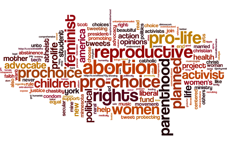
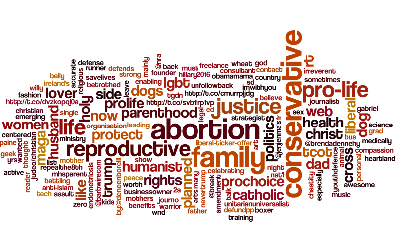
Pro-Remain	Pro-Leave
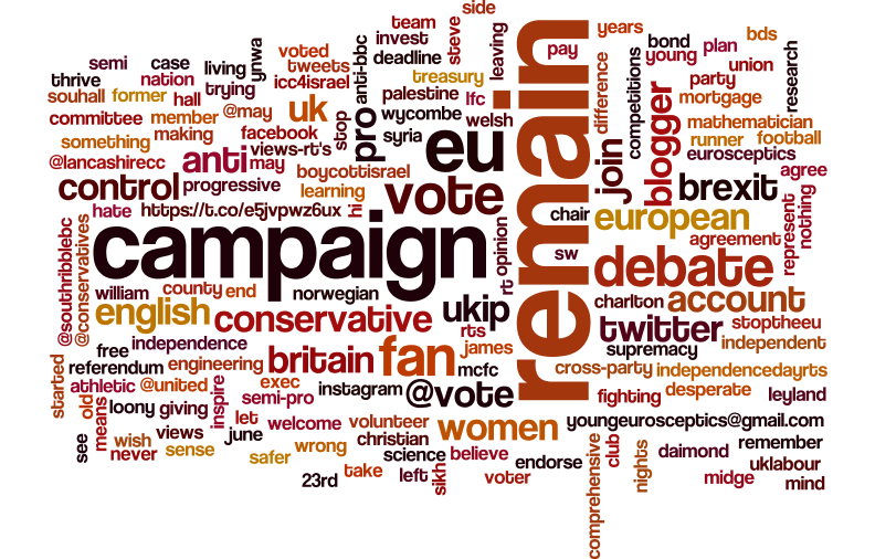
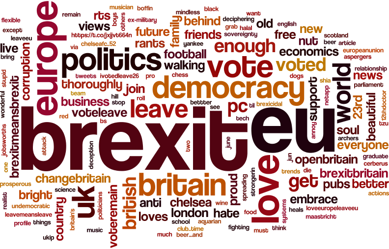
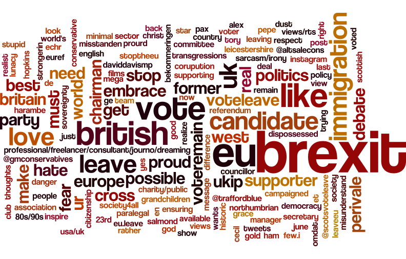
Pro-Fracking	Anti-Fracking
Pro-iPhone	Pro-Samsung
Pro-Obamacare	Anti-Obamacare
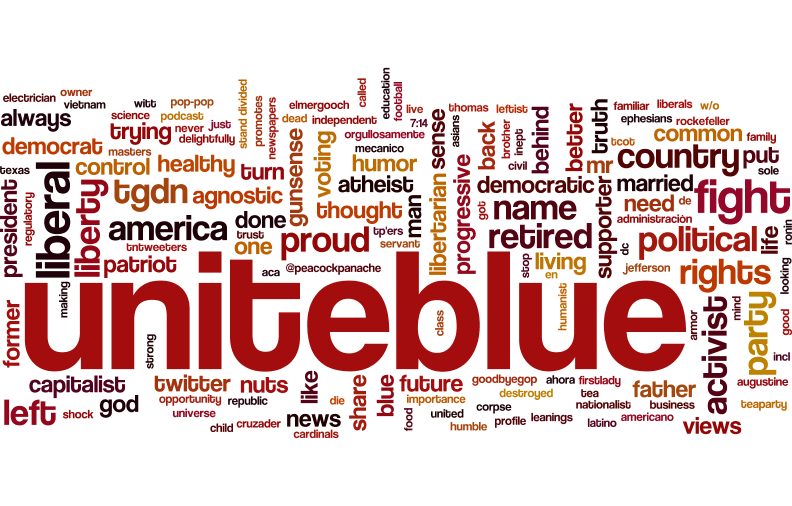
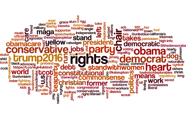
Pro-Hillary	Pro-Trump

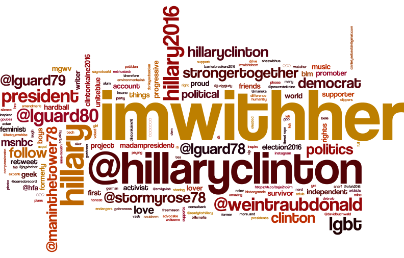
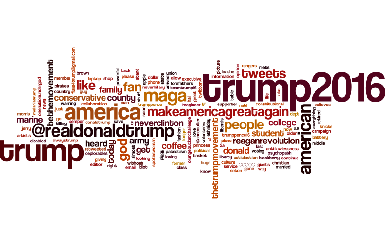
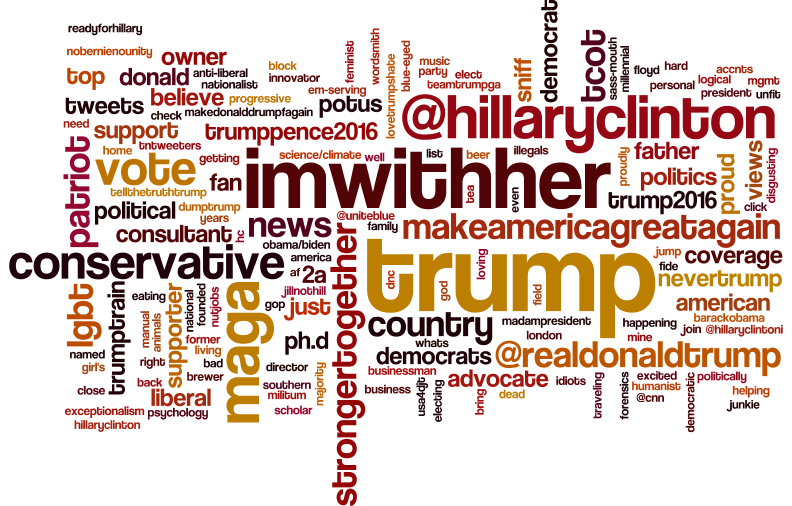
Figure 6: Word clouds of the profiles for the initial seeds, and profiles selected by Hedge.

References

- Adamic and Glance [2005] L. A. Adamic and N. Glance. The political blogosphere and the 2004 us election: divided they blog. In LinkKDD, pages 36–43, 2005.
- Akoglu [2014] L. Akoglu. Quantifying political polarity based on bipartite opinion networks. In ICWSM, 2014.
- Alon et al. [2010] N. Alon, M. Feldman, A. D. Procaccia, and M. Tennenholtz. A note on competitive diffusion through social networks. IPL, 110(6):221–225, 2010.
- Apt and Markakis [2011] K. R. Apt and E. Markakis. Diffusion in social networks with competing products. In SAGT, pages 212–223, 2011.
- Beutel et al. [2012] A. Beutel, B. A. Prakash, R. Rosenfeld, and C. Faloutsos. Interacting viruses in networks: can both survive? In KDD, pages 426–434, 2012.
- Bharathi et al. [2007] S. Bharathi, D. Kempe, and M. Salek. Competitive influence maximization in social networks. In WINE, 2007.
- Borodin et al. [2010] A. Borodin, Y. Filmus, and J. Oren. Threshold models for competitive influence in social networks. In WINE, 2010.
- Borodin et al. [2017] A. Borodin, M. Braverman, B. Lucier, and J. Oren. Strategyproof mechanisms for competitive influence in networks. Algorithmica, 78(2):425–452, 2017.
- Broecheler et al. [2010] M. Broecheler, P. Shakarian, and V. Subrahmanian. A scalable framework for modeling competitive diffusion in social networks. In ICSC, pages 295–302, 2010.
- Budak et al. [2011] C. Budak, D. Agrawal, and A. El Abbadi. Limiting the spread of misinformation in social networks. In WWW, pages 665–674, 2011.
- Carnes et al. [2007] T. Carnes, C. Nagarajan, S. M. Wild, and A. Van Zuylen. Maximizing influence in a competitive social network: a follower’s perspective. In EC, 2007.
- Conover et al. [2011] M. Conover, J. Ratkiewicz, M. Francisco, B. Gonçalves, F. Menczer, and A. Flammini. Political Polarization on Twitter. In ICWSM, 2011.
- Del Vicario et al. [2015] M. Del Vicario, A. Bessi, F. Zollo, F. Petroni, A. Scala, G. Caldarelli, H. E. Stanley, and W. Quattrociocchi. Echo chambers in the age of misinformation. arXiv:1509.00189, 2015.
- Du et al. [2013] N. Du, L. Song, M. G. Rodriguez, and H. Zha. Scalable influence estimation in continuous-time diffusion networks. In Advances in neural information processing systems, pages 3147–3155, 2013.
- Dubey et al. [2006] P. Dubey, R. Garg, and B. De Meyer. Competing for customers in a social network: The quasi-linear case. In WINE, 2006.
- Garimella et al. [2016] K. Garimella, G. De Francisci Morales, A. Gionis, and M. Mathioudakis. Quantifying controversy in social media. In WSDM, pages 33–42, 2016.
- Garimella et al. [2017] K. Garimella, G. De Francisci Morales, A. Gionis, and M. Mathioudakis. Reducing controversy by connecting oppposing views. In WSDM, 2017.
- Garrett [2009] R. K. Garrett. Echo chambers online?: Politically motivated selective exposure among internet news users1. JCMC, 14(2):265–285, 2009.
- Gomez Rodriguez et al. [2010] M. Gomez Rodriguez, J. Leskovec, and A. Krause. Inferring networks of diffusion and influence. In Proceedings of the 16th ACM SIGKDD international conference on Knowledge discovery and data mining, pages 1019–1028. ACM, 2010.
- Gottfried and Shearer [2016] J. Gottfried and E. Shearer. News use across social media platforms 2016. Pew Research Center, 2016.
- Goyal et al. [2014] S. Goyal, H. Heidari, and M. Kearns. Competitive contagion in networks. Games and Economic Behavior, 2014.
- Guerra et al. [2013] P. H. C. Guerra, W. Meira Jr, C. Cardie, and R. Kleinberg. A measure of polarization on social media networks based on community boundaries. In ICWSM, 2013.
- Jie et al. [2016] R. Jie, J. Qiao, G. Xu, and Y. Meng. A study on the interaction between two rumors in homogeneous complex networks under symmetric conditions. Physica A, 454:129–142, 2016.
- Kempe et al. [2003] D. Kempe, J. Kleinberg, and É. Tardos. Maximizing the spread of influence through a social network. In KDD, pages 137–146, 2003.
- Kostka et al. [2008] J. Kostka, Y. A. Oswald, and R. Wattenhofer. Word of mouth: Rumor dissemination in social networks. In SIROCCO, pages 185–196, 2008.
- Liao and Fu [2014a] Q. V. Liao and W.-T. Fu. Can you hear me now?: mitigating the echo chamber effect by source position indicators. In CSCW, pages 184–196, 2014a.
- Liao and Fu [2014b] Q. V. Liao and W.-T. Fu. Expert voices in echo chambers: effects of source expertise indicators on exposure to diverse opinions. In CHI, pages 2745–2754, 2014b.
- Lu et al. [2015a] H. Lu, J. Caverlee, and W. Niu. Biaswatch: A lightweight system for discovering and tracking topic-sensitive opinion bias in social media. In CIKM, pages 213–222, 2015a.
- Lu et al. [2015b] W. Lu, W. Chen, and L. V. Lakshmanan. From competition to complementarity: comparative influence diffusion and maximization. PVLDB, 9(2):60–71, 2015b.
- Morales et al. [2015] A. Morales, J. Borondo, J. Losada, and R. Benito. Measuring political polarization: Twitter shows the two sides of Venezuela. Chaos, 25(3), 2015.
- Munson et al. [2013] S. A. Munson, S. Y. Lee, and P. Resnick. Encouraging reading of diverse political viewpoints with a browser widget. In ICWSM, 2013.
- Myers and Leskovec [2012] S. A. Myers and J. Leskovec. Clash of the contagions: Cooperation and competition in information diffusion. In ICDM, pages 539–548, 2012.
- Nemhauser et al. [1978] G. Nemhauser, L. Wolsey, and M. Fisher. An analysis of approximations for maximizing submodular set functions – I. Mathematical Programming, 14(1):265–294, 1978.
- Nguyen et al. [2012] N. P. Nguyen, G. Yan, M. T. Thai, and S. Eidenbenz. Containment of misinformation spread in online social networks. In Web Science, pages 213–222, 2012.
- Nikolov et al. [2015] D. Nikolov, D. F. Oliveira, A. Flammini, and F. Menczer. Measuring online social bubbles. PeerJ Computer Science, 1:e38, 2015.
- Pariser [2011] E. Pariser. The filter bubble: What the Internet is hiding from you. Penguin UK, 2011.
- Tzoumas et al. [2012] V. Tzoumas, C. Amanatidis, and E. Markakis. A game-theoretic analysis of a competitive diffusion process over social networks. In WINE, 2012.
- Valera and Gomez-Rodriguez [2015] I. Valera and M. Gomez-Rodriguez. Modeling adoption of competing products and conventions in social media. In ICDM, 2015.
- Vydiswaran et al. [2015] V. Vydiswaran, C. Zhai, D. Roth, and P. Pirolli. Overcoming bias to learn about controversial topics. JAIST, 2015.