Multiscale Finite Element Modeling of Nonlinear Magnetoquasistatic Problems using Magnetic Induction Conforming Formulations

Abstract

In this paper we develop magnetic induction conforming multiscale formulations for magnetoquasistatic problems involving periodic materials. The formulations are derived using the periodic homogenization theory and applied within a heterogeneous multiscale approach. Therefore the fine-scale problem is replaced by a macroscale problem defined on a coarse mesh that covers the entire domain and many mesoscale problems defined on finely-meshed small areas around some points of interest of the macroscale mesh (e.g. numerical quadrature points). The exchange of information between these macro and meso problems is thoroughly explained in this paper. For the sake of validation, we consider a two-dimensional geometry of an idealized periodic soft magnetic composite.

35K55, 65M60, 65N30, 78A25, 78A30, 78A48, 78M10, 78M35, 78M40.

1 Introduction

The use of numerical methods for solving electromagnetic problems is nowadays widespread. Indeed, analytical solutions of Maxwell’s equations are not always available when facing the complexity of real-life devices with complicated geometries and materials exhibiting a possibly nonlinear or hysteretic behaviour. In this paper we are interested in multiscale magnetoquasistatic (MQS) problems. These problems arise from Maxwell’s equations when the wavelength of the exciting source is much greater than the size of the structure so that the displacement currents can be neglected. This is the model that describes the physics of most electric power systems: electric generators, motors and transformers.

The finite element (FE) method is a frequently-used numerical method for solving MQS problems for its easiness to handle problems involving both nonlinearities and complex geometries. To this end, a mesh of the structure is generated and Maxwell’s equations are weakly verified on average on elements of the mesh, which is ensured by integrating these equations elementwise. If the problem is well-posed, the finer the mesh, the more accurate the numerical solution.

Soft ferrites, lamination stacks and soft magnetic composites (SMC) are multiscale materials used in MQS applications. For instance, soft ferrites help reducing the magnetic losses in high-frequency transformers; the cores of electrotechnical devices are laminated to limit the eddy current losses; and the SMCs ease the manufacturing of three-dimensional paths in electrical machines.

For problems involving such multiscale materials, the application of classical numerical methods such as the FE method becomes prohibitive in terms of the computational resources (time and memory) storage whence the use of homogenization and multiscale methods. Using these methods, the multiscale problem is replaced by the homogenized problem defined on the homogeneous domain with a slowly varying fields. The performance of homogenization and multiscale methods for MQS problems can be compared by evaluating their ability to

• derive a homogenized problem that can be easily solved;

• handle nonlinearities;

• deal with materials with complex microstructures;

• deal with partial differential equations involving curl operators;

• compute global quantities such as the eddy currents or magnetic losses.

• recover local fields at critical points of interest;

The first homogenization approach used to analytically characterize properties of composites materials was based on mixing rules [47, 63]. More elaborate theoretical methods such as the asymptotic expansion method [7], the G-convergence [50, 64], the $\Gamma$-convergence [22, 15, 21], the two-scale convergence [51, 67] and the periodic unfolding methods [18, 19] allow to construct the homogenized problem and determine the associated constitutive laws. Equations resulting from these methods can be used to develop multiscale methods. A non-exhaustive list of these multiscale methods include the mean-field homogenization method [16, 20], the multiscale finite element method–MsFEM [41, 32], the variational multiscale method–VMS [17, 44] and the heterogeneous multiscale method–HMM [31, 1, 27]. In electromagnetism such methods have been developed mainly for materials with linear [9, 10, 38, 48, 14, 13] and nonlinear [39, 5, 12] magnetic material laws. While some preliminary results concerning electromagnetic hysteresis can be found in [61], there is to date no generic multiscale method able to accurately handle hysteretic materials in complex geometrical configurations.

In this paper we develop such a multiscale method to treat magnetoquasistatic problems involving multiscale materials that can exhibit linear, nonlinear or hysteretic behaviour with the main focus on the development of weak formulations for the homogenized problem. Using results from the theory of homogenization for nonlinear electromagnetic multiscale problem obtained by Visintin, we develop the magnetic vector potential formulations for the multiscale, the macroscale and the mesoscale problems. The formulations are then validated on simple 2D geometry. The multiscale method is inspired by the HMM and is based on the scale separation assumption $\varepsilon\ll 1$ where $\varepsilon=l/L$ is the ratio between the smallest scale $l$ and the scale of the material or the characteristic length of external loadings $L$. The fine-scale problem is replaced by a macroscale problem defined on a coarse mesh covering the entire domain and many mesoscale problems that are defined on small, finely meshed areas around some points of interest of the macroscale mesh (e.g. numerical quadrature points). The transfer of information between these problems is performed during the upscaling and the downscaling stages that will be detailed hereafter.

The paper comprises five sections. In Section 2 we derive the MQS multiscale and homogenized problems from the multiscale problem that was studied by Visintin in [65, 67]. In Section 3 we derive the weak forms of the multiscale MQS problem. Section 4 deals with the multiscale weak formulations for homogenized MQS problems. Starting from the distributional equations that govern the fields of the MQS homogenized problem we develop magnetic vector potential formulations for the macroscale and the mesoscale problems. Scale transitions are also thoroughly investigated. Section 5 concerns the application of the theory to a simple but representative two-dimensional problem: the modeling of a soft magnetic composite. Conclusions are drawn in the last section.

2 Derivation of the homogenized magnetoquasistatic problem

In this section, the homogenized magnetoquasistatic (MQS) problem is derived. The derivation uses two main ingredients: the MQS assumptions which makes it possible to neglect the displacement currents and the homogenization of the corresponding multiscale problem. The derivation of this paper is made easier by applying the MQS assumptions to the homogenized parabolic hyperbolic (PH) multiscale problem that was already carried out in [65, 67] instead of applying the homogenization theory to the parabolic elliptic (PE) multiscale problem derived from the PH multiscale under appropriate assumptions (see Figure 1). In [65, 67], existence and uniqueness of the solution was proved via the approximation by time-discretization, the derivation of a priori estimates, and the passage to the limit via compensated compactness and compactness by strict convexity. The homogenized problem was then derived using the two-scale convergence theory for the fields and the convergence of functionals used to define constitutive laws. In Section 2.1 we recall Maxwell’s equations that govern the evolution of electromagnetic fields and we define the function spaces used for solving these equations in the weak sense. In Section 2.2, we recall the PH multiscale problem and its homogenization as done in [65, 67]. This homogenized problem is then used in Section 2.3 for the derivation of the homogenized parabolic elliptic (PE) problem. In the rest of the section, we use the capital letters P, H end E to denote the parabolic, hyperbolic and elliptic problems, respectively. Thus, the PH multiscale problem denotes the parabolic hyperbolic multiscale problem whereas the PE–PH homogenized problem denotes the homogenized problem with a PE problem at the coarse scale and a PH problem are the fine scale. The PE problem corresponds to the MQS problem.

2.1 Maxwell’s equations and the function spaces

Consider the electromagnetic problem in an open domain $\Omega_{T}:=\Omega\times\mathcal{I}$ with $\Omega\subseteq\mathbb{R}^{3}$ and $\mathcal{I}=(0,T]\subset\mathbb{R}$. The electromagnetic fields are governed by the following Maxwell equations and constitutive laws [8, 11, 42]:

(2.1 a-c) $$\text{\text{\bf curl}}{}\,{\mbox{\boldmath$h$}}=\mbox{\boldmath$j$}+\mbox{\boldmath$j$}_{s}+\epsilon\partial_{t}\mbox{\boldmath$e$},\quad\text{\text{\bf curl}}{}\,{\mbox{\boldmath$e$}}=-\partial_{t}\mbox{\boldmath$b$},\quad\text{\text{div}}{}\,{\mbox{\boldmath$b$}}=0\hskip 14.22636pt\textrm{ in }\Omega\times\mathcal{I},$$

(2.2 a-b) $$\mbox{\boldmath$b$}(\mbox{\boldmath$x$},t)=\boldsymbol{\mathcal{B}}(\mbox{\boldmath$h$}(\mbox{\boldmath$x$},t),\mbox{\boldmath$x$}),\quad\mbox{\boldmath$j$}(\mbox{\boldmath$x$},t)=\boldsymbol{\mathcal{J}}(\mbox{\boldmath$e$}(\mbox{\boldmath$x$},t),\mbox{\boldmath$x$})\hskip 14.22636pt\forall(\mbox{\boldmath$x$},t)\in\Omega\times\mathcal{I}.$$

The field $h$ is the magnetic field, $b$ the magnetic flux density, $j$ the electric current density, $\mbox{\boldmath$j$}_{s}$ the imposed electric current density (source) and $e$ the electric field. The material laws (2.2 a-b) are expressed in terms of the mappings $\boldsymbol{\mathcal{B}}:\mathbb{R}^{3}\times\Omega\rightarrow\mathbb{R}^{3}$ and $\boldsymbol{\mathcal{J}}:\mathbb{R}^{3}\times\Omega\rightarrow\mathbb{R}^{3}$, linear or not, accounting for the magnetic and electric behaviour, respectively. The domain $\Omega$ is subdivided into conducting ($\Omega_{c}$) and nonconducting ($\Omega_{c}^{C}$) parts, the former being where eddy currents can appear. The boundary of the domain $\Omega$ is denoted $\Gamma$. In Sections 3 and 4 we derive the weak solution sof the MQS problem using the magnetic vector potential formulations [4, 43, 60, 3]. In Sections 3 and 4, some structural restrictions on the computational domain are assumed for the existence and the uniqueness of the solution [60, 3, 4]. The domain $\Omega$ is assumed to be simply connected with a Lipschitz connected boundary $\Gamma$. The conducting domain $\Omega_{c}$ is an open subset strictly contained in $\Omega$ which can be connected or not. In the latter case, $\Omega_{c}=\cup_{i=1}^{m}\Omega_{c}^{i}$ where $\Omega_{c}^{i}$, i = 1, 2, …, m are connected components of $\Omega_{c}$. For simplicity we assume the non-conducting domain $\Omega_{c}^{C}$ to be connected. The case of a non-connected $\Omega_{c}^{C}$ can be also easily treated. The system of equations must further be completed by an initial condition on the magnetic flux density assumed to be divergence-free, i.e., $\text{\text{div}}{}\,{\mbox{\boldmath$b$}^{0}}=0$. The superscript ⁰ is used to denote initial condition, i.e., $\mbox{\boldmath$b$}^{0}=\mbox{\boldmath$b$}(\cdot,0)$. This conditions together with (2.1 a-c b) naturally imply Gauß  magnetic law (2.1 a-c c). In the rest of this section, we ignore Gauß  magnetic law which is automatically fulfilled under Faraday’s equation (2.1 a-c b) together with this initial condition $\text{\text{div}}{}\,{\mbox{\boldmath$b$}^{0}}=0$ (see [65, 67]).

The weak solutions the fullscale, the macroscale and the mesoscale problems must belong to the right function spaces. For almost every $t\in\mathcal{I}$, these functions spaces are defined as the domains of the differential operators $\text{\bf grad},\text{\bf curl}$ and div with appropriate non-homogeneous boundary conditions prescribed on the boundary $\Gamma$:

(2.3) $$H^{1}(\Omega) :=\{u\in L^{2}(\Omega):\text{\text{\bf grad}}{}\,{u}\in\boldsymbol{L}^{2}(\Omega)\},$$

(2.4) $$\boldsymbol{H}(\text{\bf curl};\Omega) :=\{\boldsymbol{u}\in\boldsymbol{L}^{2}(\Omega):\text{\text{\bf curl}}{}\,{\boldsymbol{u}}\in\boldsymbol{L}^{2}(\Omega)\},$$

(2.5) $$\boldsymbol{H}(\text{div};\Omega) :=\{\boldsymbol{u}\in\boldsymbol{L}^{2}(\Omega):\text{\text{div}}{}\,{\boldsymbol{u}}\in L^{2}(\Omega).$$

The spaces $H^{1}_{0}(\Omega)$, $\boldsymbol{H}_{0}(\text{\bf curl};\Omega)$, $\boldsymbol{H}_{0}(\text{div};\Omega)$ denote the same spaces as the corresponding spaces in (2.3)–(2.5) with traces equal to zero, i.e.,

(2.6) $$H^{1}_{0}(\Omega) :=\{u\in H^{1}(\Omega),u|_{\Gamma}=0\},$$

(2.7) $$\boldsymbol{H}_{0}(\text{\bf curl};\Omega) :=\{\boldsymbol{u}\in\boldsymbol{H}(\text{\bf curl};\Omega),\mbox{\boldmath$n$}\times\mbox{\boldmath$u$}|_{\Gamma}=\boldsymbol{0}\},$$

(2.8) $$\boldsymbol{H}_{0}(\text{div};\Omega) :=\{\boldsymbol{u}\in\boldsymbol{H}(\text{div};\Omega),\mbox{\boldmath$n$}\cdot\mbox{\boldmath$u$}|_{\Gamma}=0\}.$$

The spaces $\boldsymbol{H}(\textbf{curl}\,\boldsymbol{0};\Omega)$, $\boldsymbol{H}(\textbf{div}\,0;\Omega)$ denote the nullspace of the operators curl and div, respectively. In Sections 3 and 4 we consider the following Bochner spaces for the potentials, solution of the multiscale and the macroscale problems:

(2.9) $$\boldsymbol{L}^{2}(0,T;\boldsymbol{V})\qquad\text{ and }\qquad\boldsymbol{L}^{2}(0,T;\boldsymbol{V}^{\ast}),$$

where $\boldsymbol{V}$ can be any vector space (in Sections 3 and 4 we use $\boldsymbol{V}:=\boldsymbol{H}_{0}(\text{\bf curl};\Omega)$) and $\boldsymbol{V}^{\ast}$ is the dual of $\boldsymbol{V}$. The mesoscale problem leads to the solutions that belong to the spaces:

(2.10) $$\boldsymbol{L}^{2}(\mathbb{R}_{T}^{3};\boldsymbol{W}):=\left\{\mbox{\boldmath$u$}:\mathbb{R}_{T}^{3}\rightarrow\boldsymbol{W}:\displaystyle{{\color[rgb]{1,1,1}\left(\int_{\mathbb{R}_{T}^{3}}\right)^{\frac{1}{2}}}}\right.\\ \left.\|\mbox{\boldmath$u$}\|_{\boldsymbol{L}^{2}(\mathbb{R}_{T}^{3}:\boldsymbol{W})}:=\left(\int_{\mathbb{R}_{T}^{3}}\left\|\mbox{\boldmath$u$}(\mbox{\boldmath$x$},t)\right\|_{\boldsymbol{W}}^{2}\text{d}t\,\text{d}x\right)^{\frac{1}{2}}<\infty\right\},\vspace{-2mm}$$

where the separable Banach space $\boldsymbol{W}$ is defined on the mesoscale domain $Y\equiv\Omega_{m}$. For the homogenized PH problem, two spaces were used in place of $\boldsymbol{W}$: the nullspaces $\boldsymbol{H}(\textbf{curl}\,\boldsymbol{0};\mathcal{Y})$ and $\boldsymbol{H}(\textbf{div}\,0;\mathcal{Y})$. The symbol $\mathcal{Y}$ is used for functions defined on $Y$ with periodic boundary conditions.

2.2 Homogenization of the Parabolic Hyperbolic multiscale problem

From now on, we consider $\Omega=\mathbb{R}^{3}$ and derive the parabolic hyperbolic multiscale problem along the lines of [65, 67].

Problem 2.1 (Parabolic–Hyperbolic (PH) multiscale problem).

The PH multiscale problem was derived from Maxwell’s equation by neglecting the displacement currents with respect to the eddy currents in the conducting domain (i.e., $\epsilon\partial_{t}\mbox{\boldmath$e$}^{\varepsilon}\ll\mbox{\boldmath$j$}^{\varepsilon}$ in $\Omega_{c}$).

(2.11 a-b) $$\text{\text{\bf curl}}{}\,{\mbox{\boldmath$h$}^{\varepsilon}}=\mbox{\boldmath$j$}^{\varepsilon}+\mbox{\boldmath$j$}_{s}+(1-\chi_{{}_{\Omega_{c}}})\epsilon^{\varepsilon}\,\partial_{t}\mbox{\boldmath$e$}^{\varepsilon},\qquad\text{\text{\bf curl}}{}\,{\mbox{\boldmath$e$}^{\varepsilon}}=-\partial_{t}\mbox{\boldmath$b$}^{\varepsilon},$$

(2.12 a-b) $$\mbox{\boldmath$b$}^{\varepsilon}(\mbox{\boldmath$x$},t)=\boldsymbol{\mathcal{B}}^{\varepsilon}(\mbox{\boldmath$h$}^{\varepsilon}(\mbox{\boldmath$x$},t),\mbox{\boldmath$x$}),\,\,\mbox{\boldmath$j$}^{\varepsilon}(\mbox{\boldmath$x$},t)=\boldsymbol{\mathcal{J}}^{\varepsilon}(\mbox{\boldmath$e$}^{\varepsilon}(\mbox{\boldmath$x$},t),\mbox{\boldmath$x$})\,\,\,\,\forall(\mbox{\boldmath$x$},t)\in\mathbb{R}_{T}^{3}$$

where the function $\chi_{{}_{\Omega_{c}}}$ is the characteristic function, different from zero only on the conducting domain $\Omega_{c}$. The superscript ^ε is used to denote the multiscale dependency of the fields. All derivatives are defined in the distribution sense.

In [65, 67], Gauß  magnetic law $\text{\text{div}}{}\,{\mbox{\boldmath$b$}^{\varepsilon}}=0$ was ensured by imposing the initial condition on $\mbox{\boldmath$b$}^{\varepsilon 0}$ such that $\text{\text{div}}{}\,{\mbox{\boldmath$b$}^{\varepsilon 0}}=0$. The material laws (2.2 a-b) are expressed in terms of the mappings $\boldsymbol{\mathcal{B}}^{\varepsilon}:\mathbb{R}^{3}\times\Omega\rightarrow\mathbb{R}^{3}$ and $\boldsymbol{\mathcal{J}}^{\varepsilon}:\mathbb{R}^{3}\times\Omega\rightarrow\mathbb{R}^{3}$ defined by:

(2.13) $$\boldsymbol{\mathcal{B}}^{\varepsilon}(\mbox{\boldmath$h$}^{\varepsilon},\mbox{\boldmath$x$})=\boldsymbol{\mathcal{\bar{B}}}(\mbox{\boldmath$h$}^{\varepsilon},\mbox{\boldmath$x$},\mbox{\boldmath$x$}/\varepsilon),\qquad\boldsymbol{\mathcal{J}}^{\varepsilon}(\mbox{\boldmath$e$}^{\varepsilon},\mbox{\boldmath$x$})=\boldsymbol{\mathcal{\bar{J}}}(\mbox{\boldmath$e$}^{\varepsilon},\mbox{\boldmath$x$},\mbox{\boldmath$x$}/\varepsilon),$$

where the operators $\boldsymbol{\mathcal{\bar{B}}}:\mathbb{R}^{3}\times\Omega\times Y\rightarrow\mathbb{R}^{3}$ and $\boldsymbol{\mathcal{\bar{J}}}:\mathbb{R}^{3}\times\Omega\times\times Y\rightarrow\mathbb{R}^{3}$ are used to represent two-scale composite materials for which the characteristic length at the mesoscale is $\varepsilon$. By abuse of notation, we use $\boldsymbol{\mathcal{B}}$ and $\boldsymbol{\mathcal{J}}$ instead of $\boldsymbol{\mathcal{\bar{B}}}$ and $\boldsymbol{\mathcal{\bar{J}}}$ in the rest of the text. For the analytical and theoretical study of the multiscale Problem 2.1 we assume that the nonlinear mapping $\boldsymbol{\mathcal{B}}$ is maximal monotone and therefore it can be derived by the minimization of a convex, lower-semicontinous functional. It also has an inverse ${\boldsymbol{\mathcal{B}}^{-1}\equiv\boldsymbol{\mathcal{H}}}$ that can be derived from a conjuguate convex, lower semi-continuous functional [33, 35, 59]. This covers cases of linear and nonlinear reversible magnetic laws. However, one of the major advantages of the computational homogenization approach proposed in Section 4 is the inclusion of hysteretic laws in the numerical model by means of classical hysteresis models (e.g. Preisach, Jiles-Atherton, etc.). We will thus lift this hypothesis once we consider the computational framework. We will still assume that the mapping $\boldsymbol{\mathcal{J}}$ is maximal monotone and has an inverse $\boldsymbol{\mathcal{J}}^{-1}\equiv\boldsymbol{\mathcal{E}}$. In practice, this assumption holds as the materials we consider in this paper are electrically linear.

Problem 2.1 has been extensively analyzed. A homogenized problem with coarse and fine problems was derived considering some assumptions on the constitutive laws, the initial conditions (IC) and the current source $\mbox{\boldmath$j$}_{s}$. These assumptions are recalled in Assumptions 2.14–3

Assumption 1 (Regularity of the IC and the sources).

Assume that the
initial conditions $\mbox{\boldmath$b$}^{\varepsilon 0}$ and $\mbox{\boldmath$e$}^{\varepsilon 0}$ and the source $\mbox{\boldmath$j$}_{s}$ fulfill the following regularity conditions:

(2.14 a-e) $$\mbox{\boldmath$b$}^{\varepsilon 0}\in\boldsymbol{L}^{2}(\mathbb{R}^{3}),\,\,\,\mbox{\boldmath$e$}^{\varepsilon 0}\in\boldsymbol{L}^{2}(\Omega_{c}^{C}),\,\,\,\mbox{\boldmath$j$}_{s}\in\boldsymbol{L}^{2}(\Omega_{s}\times\mathcal{I}),\,\,\,\text{\text{div}}{}\,{\mbox{\boldmath$b$}^{\varepsilon 0}}=0,\,\,\,\text{\text{div}}{}\,{\mbox{\boldmath$j$}_{s}}=0.$$

Equation (2.14 a-e d) together with (2.11 a-b b) ensures Gauß  magnetic law $\text{\text{div}}{}\,{\mbox{\boldmath$b$}^{\varepsilon}}=0$.

Assumption 2 (Assumptions on the constitutive laws).

Assume that the
electrical law is given by $\mbox{\boldmath$j$}^{\varepsilon}=\sigma^{\varepsilon}\,\mbox{\boldmath$e$}^{\varepsilon}$ where the electrical conductivity $\sigma^{\varepsilon}$ is definite positive in $\Omega_{c}$ and that the mapping $\boldsymbol{\mathcal{B}}$ is maximal monotone.

These restrictions on the mappings cover a wide range of material laws usually encountered in applications. They cover the linear electrical materials, the linear and the nonlinear reversible magnetic materials as well as soft magnetic materials for which the hysteresis loop can be approximated using the maximal monotone operators. However, the hard magnetic materials are not covered.

Assumption 3 (Convergence of the initial conditions).

Assume that the
initial conditions $\mbox{\boldmath$b$}_{0}^{\varepsilon}$ and $\mbox{\boldmath$e$}_{0}^{\varepsilon}$ converge in the classical and the two-scale senses, i.e.:

(2.15 a-b) $$\mbox{\boldmath$b$}^{\varepsilon 0}\underset{2}{\rightharpoonup}\mbox{\boldmath$b$}_{0}^{0}\,\,\emph{\text{ in }}\,\,\boldsymbol{L}^{2}(\mathbb{R}^{3}\times\mathcal{Y}),\qquad \mbox{\boldmath$b$}^{\varepsilon 0}\rightharpoonup\left<\mbox{\boldmath$b$}_{0}^{0}\right>_{Y}=\mbox{\boldmath$b$}_{M}^{0}\,\,\emph{\text{ in }}\,\,\boldsymbol{L}^{2}(\mathbb{R}^{3}),$$

(2.16 a-b) $$\mbox{\boldmath$e$}^{\varepsilon 0}\underset{2}{\rightharpoonup}\mbox{\boldmath$e$}_{0}^{0}\,\,\emph{\text{ in }}\,\,\boldsymbol{L}^{2}(\Omega_{c}^{C}\times\mathcal{Y}),\qquad \mbox{\boldmath$e$}^{\varepsilon 0}\rightharpoonup\left<\mbox{\boldmath$e$}_{0}^{0}\right>_{Y}=\mbox{\boldmath$e$}_{M}^{0}\,\,\emph{\text{ in }}\,\,\boldsymbol{L}^{2}(\Omega_{c}^{C}).$$

These fields are used as initial conditions for the fine and the coarse problem, respectively. The curly brackets $\left<\mbox{\boldmath$f$}\right>_{Y}$ are used to denote the average of the function $f$ over the cell domain $Y$, i.e.,

$$\left<\mbox{\boldmath$f$}\right>_{Y}=\frac{1}{|Y|}\int_{Y}\mbox{\boldmath$f$}\text{d}y=\frac{1}{|\Omega_{m}|}\int_{\Omega_{m}}\mbox{\boldmath$f$}\text{d}y=\left<\mbox{\boldmath$f$}\right>_{\Omega_{m}}$$

where $|Y|$ is used to denote the volume of the domain $Y\equiv\Omega_{m}$.

Using Assumption 2.14 for the IC and the source term and Assumption 2 for the constitutive laws, the following PH–PH homogenized problem was derived from the multiscale Problem 2.1 ([67]):

Problem 2.2 (PH–PH homogenized problem).

The PH–PH homogenized
problem has been derived from Problem 2.1 with the following two coarse and fine problems:
Coarse problem: find $\mbox{\boldmath$h$}_{M},\mbox{\boldmath$e$}_{M},\mbox{\boldmath$b$}_{M},\mbox{\boldmath$j$}_{M}\in\boldsymbol{L}^{2}(\mathbb{R}_{T}^{3})$ such that

(2.17 a-b) $$\text{\text{\bf curl}}{{}_{x}}\,{\mbox{\boldmath$h$}_{M}}=\mbox{\boldmath$j$}_{M}+\mbox{\boldmath$j$}_{s}+(1-\chi_{{}_{\Omega_{c}}})\epsilon_{M}\partial_{t}\mbox{\boldmath$e$}_{M},\,\,\,\,\text{\text{\bf curl}}{{}_{x}}\,{\mbox{\boldmath$e$}_{M}}=-\partial_{t}\mbox{\boldmath$b$}_{M},$$

(2.18 a-b) $$\mbox{\boldmath$b$}_{M}=\boldsymbol{\mathcal{B}}_{M}(\mbox{\boldmath$h$}_{M},\mbox{\boldmath$x$}),\,\,\mbox{\boldmath$j$}_{M}=\boldsymbol{\mathcal{J}}_{M}(\mbox{\boldmath$e$}_{M},\mbox{\boldmath$x$}),\,\,\text{ for a.e. }(\mbox{\boldmath$x$},t)\in\mathbb{R}^{3}\times\mathcal{I}.$$

Fine problem: find $\mbox{\boldmath$h$}_{0},\mbox{\boldmath$e$}_{0}\in\boldsymbol{L}^{2}(\mathbb{R}_{T}^{3}\!\!:\!\!\boldsymbol{H}(\textbf{curl}\,\boldsymbol{0};\mathcal{Y}))$ and $\mbox{\boldmath$h$}_{1},\mbox{\boldmath$e$}_{1},\mbox{\boldmath$b$}_{0},\mbox{\boldmath$j$}_{0}\in\boldsymbol{L}^{2}(\mathbb{R}_{T}^{3}\!\!:\!\!\boldsymbol{H}(\textbf{div}\,0;\mathcal{Y}))$ such that

(2.19a) $$\text{\text{\bf curl}}{{}_{x}}\,{\mbox{\boldmath$h$}_{M}}+\text{\text{\bf curl}}{{}_{y}}\,{\mbox{\boldmath$h$}_{1}}=\mbox{\boldmath$j$}_{0}+(1-\chi_{{}_{\Omega_{c}}})\epsilon\partial_{t}\mbox{\boldmath$e$}_{0},\\ \text{\text{\bf curl}}{{}_{x}}\,{\mbox{\boldmath$e$}_{M}}+\text{\text{\bf curl}}{{}_{y}}\,{\mbox{\boldmath$e$}_{1}}=-\partial_{t}\mbox{\boldmath$b$}_{0},{\color[rgb]{1,1,1}Fillingtext}$$

(2.20 a-b) $$\mbox{\boldmath$b$}_{0}=\boldsymbol{\mathcal{B}}(\mbox{\boldmath$h$}_{0},\mbox{\boldmath$x$},\mbox{\boldmath$y$}),\,\,\mbox{\boldmath$j$}_{0}=\boldsymbol{\mathcal{J}}(\mbox{\boldmath$e$}_{0},\mbox{\boldmath$x$},\mbox{\boldmath$y$}),\,\,\text{ for a.e. }(\mbox{\boldmath$x$},\mbox{\boldmath$y$},t)\in\mathbb{R}^{3}\times Y\times\mathcal{I}_{t}.$$

The macroscale fields are obtained as averages of the zero order terms, i.e., $\mbox{\boldmath$f$}_{M}=\langle{\mbox{\boldmath$f$}}_{0}\rangle_{Y}$. All the derivatives are defined in the distribution sense.

Equation (2.17 a-b b) together with $\text{\text{div}}{{}_{x}}\,{\mbox{\boldmath$b$}_{M}^{0}}=0$ imply the coarse scale Gauß  magnetic law $\text{\text{div}}{{}_{x}}\,{\mbox{\boldmath$b$}_{M}}=0$. The equations of the fine scale (2.19a a-b)–(2.20 a-b a-b) involve the nullspaces that can be decomposed as [67, 68, 57, 49]:

(2.21) $$\boldsymbol{H}(\textbf{curl}\,\boldsymbol{0};\mathcal{Y})=\mathbb{R}^{3}\,\oplus\,\boldsymbol{H}_{*}(\textbf{curl}\,\boldsymbol{0};\mathcal{Y})=\mathbb{R}^{3}\,\oplus\,\text{\bf grad}_{y}\,H^{1}_{*}(\mathcal{Y}),$$

(2.22) $$\boldsymbol{H}(\textbf{div}\,0;\mathcal{Y})=\mathbb{R}^{3}\,\oplus\,\boldsymbol{H}_{*}(\textbf{div}\,0;\mathcal{Y})=\mathbb{R}^{3}\,\oplus\,\text{\bf curl}_{y}\,\boldsymbol{H}_{*}(\text{\bf curl};\mathcal{Y}).$$

Using the decompositions in (2.21) and (2.22), each field $\mbox{\boldmath$f$}_{0}$ of $\boldsymbol{H}(\textbf{curl}\,\boldsymbol{0};\mathcal{Y})$ or $\boldsymbol{H}(\textbf{div}\,0;\mathcal{Y})$ can be written as the sum of an average value $\left<\mbox{\boldmath$f$}_{0}\right>_{Y}\in\mathbb{R}^{3}$ and a zero average perturbation $\tilde{\mbox{\boldmath$f$}}_{0}$. The second equalities in (2.21) and (2.22) are obtained using the Helmholtz decomposition of $\boldsymbol{L}^{2}_{*}(\mathcal{Y})$:

(2.23) $$\boldsymbol{L}^{2}_{*}(\mathcal{Y})=\text{\bf grad}_{y}\,H^{1}_{*}(\mathcal{Y})\,\oplus\,\text{\bf curl}_{y}\,\boldsymbol{H}_{*}(\text{\bf curl};\mathcal{Y})$$

which applies for fields with periodic boundary conditions. Indeed, the subspace of gradients of a harmonic function which appears in the general decomposition of $\boldsymbol{L}^{2}$ fields is dismissed in the case of periodic functions (2.23) and for $\Omega=\mathbb{R}^{n}$ ([24, 40]).

The decomposition (2.23) was used by Visintin for the convergence of functionals used to derive the nonlinear magnetic material laws. For almost every $(\mbox{\boldmath$x$},t)\in\mathbb{R}_{T}^{3}$, the decompositions in (2.21)–(2.22) leads to the decompositions of the first order terms $\mbox{\boldmath$e$}_{0}=\mbox{\boldmath$e$}_{M}+\text{\text{\bf grad}}{{}_{y}}\,{v_{c}}$ and $\mbox{\boldmath$b$}_{0}=\mbox{\boldmath$b$}_{M}+\text{\text{\bf curl}}{{}_{y}}\,{\mbox{\boldmath$a$}_{c}}$ with $v_{c}\in H^{1}_{*}(\mathcal{Y})$ and $\mbox{\boldmath$a$}_{c}\in\boldsymbol{H}_{*}(\text{\bf curl};\mathcal{Y})$.

If the mappings $\boldsymbol{\mathcal{B}}$ and $\boldsymbol{\mathcal{J}}$ are maximal monotone then the mappings $\boldsymbol{\mathcal{B}}_{M}$ and $\boldsymbol{\mathcal{J}}_{M}$ are also maximal monotone and derived using the approach described in the following paragraphs. Their inverses $\boldsymbol{\mathcal{H}}_{M}\equiv\boldsymbol{\mathcal{B}}_{M}^{-1}$ and $\boldsymbol{\mathcal{E}}_{M}\equiv\boldsymbol{\mathcal{J}}_{M}^{-1}$ can therefore be determined by minimizing the convex conjugate functionals and determined by means of the mesoscale problems hereafter [67].

For the mapping $\boldsymbol{\mathcal{H}}_{M}$: find $\mbox{\boldmath$a$}_{c}\in\boldsymbol{H}_{*}(\text{\bf curl};\mathcal{Y})$ such that

(2.24) $$\left(\boldsymbol{\mathcal{H}}\left(\mbox{\boldmath$b$}_{M}+\text{\text{\bf curl}}{{}_{y}}\,{\mbox{\boldmath$a$}_{c}},\mbox{\boldmath$x$},\mbox{\boldmath$y$}\right),\text{\text{\bf curl}}{{}_{y}}\,{\mbox{\boldmath$a$}_{c}^{\prime}}\right)=0\,,\qquad\forall\mbox{\boldmath$a$}_{c}^{\prime}\in\boldsymbol{H}_{*}(\text{\bf curl};\mathcal{Y})$$

and then derive: $\boldsymbol{\mathcal{H}}_{M}(\mbox{\boldmath$b$}_{M}+\boldsymbol{\mathcal{B}}_{c},\mbox{\boldmath$x$})=\langle\boldsymbol{\mathcal{H}}(\mbox{\boldmath$b$}_{M}+\boldsymbol{\mathcal{B}}_{c},\mbox{\boldmath$x$},\mbox{\boldmath$y$})\rangle_{Y}.$

For the mapping $\boldsymbol{\mathcal{J}}_{M}$: find $v_{c}\in H^{1}_{*}(\mathcal{Y})$ such that

(2.25) $$\left(\boldsymbol{\mathcal{J}}\left(\mbox{\boldmath$e$}_{M}+\text{\text{\bf grad}}{{}_{y}}\,{v_{c}},\mbox{\boldmath$x$},\mbox{\boldmath$y$}\right),\text{\text{\bf grad}}{{}_{y}}\,{v_{c}^{\prime}}\right)=0\,\qquad\forall v_{c}^{\prime}\in H^{1}_{*}(\mathcal{Y}),$$

and then derive: $\boldsymbol{\mathcal{J}}_{M}(\mbox{\boldmath$e$}_{M}+\boldsymbol{\mathcal{E}}_{c},\mbox{\boldmath$x$})=\langle\boldsymbol{\mathcal{J}}(\mbox{\boldmath$e$}_{M}+\boldsymbol{\mathcal{E}}_{c},\mbox{\boldmath$x$}\,by)\rangle_{Y}.$

The operators

(2.26) $$\boldsymbol{\mathcal{B}}_{c}:Y\times\mathbb{R}^{3}\rightarrow\boldsymbol{L}^{2}_{*}(\mathcal{Y}):(\mbox{\boldmath$y$},\mbox{\boldmath$b$}_{M})\mapsto\mbox{\boldmath$b$}_{c}=\boldsymbol{\mathcal{B}}_{c}(\mbox{\boldmath$y$},\mbox{\boldmath$b$}_{M})$$

(2.27) $$\boldsymbol{\mathcal{E}}_{c}:Y\times\mathbb{R}^{3}\rightarrow\boldsymbol{L}^{2}_{*}(\mathcal{Y}):(\mbox{\boldmath$y$},\mbox{\boldmath$e$}_{M})\mapsto\mbox{\boldmath$e$}_{c}=\boldsymbol{\mathcal{E}}_{c}(\mbox{\boldmath$y$},\mbox{\boldmath$e$}_{M})$$

are solution operators for the mesoscale problems with $\mbox{\boldmath$b$}_{c}=\boldsymbol{\mathcal{B}}_{c}(\mbox{\boldmath$y$},\mbox{\boldmath$b$}_{M})=\text{\text{\bf curl}}{{}_{y}}\,{\mbox{\boldmath$a$}_{c}}$ and $\mbox{\boldmath$e$}_{c}=\boldsymbol{\mathcal{E}}_{c}(\mbox{\boldmath$y$},\mbox{\boldmath$e$}_{M})=\text{\text{\bf grad}}{{}_{y}}\,{\mbox{\boldmath$v$}_{c}}$. If the mappings $\boldsymbol{\mathcal{H}}$ and $\boldsymbol{\mathcal{J}}$ are linear, problem (2.24)–(2.25) is equivalent to the cell problem obtained using the asymptotic expansion theory [62, 7, 68]. The dual formulation allows to define similar problems for the constituitive laws $\boldsymbol{\mathcal{B}}_{M}\equiv\boldsymbol{\mathcal{H}}_{M}^{-1}$ and $\boldsymbol{\mathcal{E}}_{M}=\boldsymbol{\mathcal{J}}_{M}^{-1}$.

2.3 Homogenization of the Parabolic Elliptic multiscale problem

The MQS problem can be derived by applying the MQS assumption to Maxwell’s equations. This assumption can be derived by comparing the following physical parameters of the problem: $L_{c}$ and $L_{f}$ which are the coarse and fine scale characteristic lengths (e.g., the sizes of the coarse and the fine domains), $\lambda_{f}$ and $\lambda_{M}$ which are the coarse and the fine wavelengths respectively and $\delta_{c}$ and $\delta_{f}$, the coarse and the fine skin depths, respectively. The wavelengths $\lambda_{f}=2\pi/(\omega\,\sqrt{\mu\epsilon})$ and $\lambda_{M}=2\pi/(\omega\,\sqrt{\mu_{M}\epsilon_{M}})$ and the skin depths are defined by $\delta_{f}=\sqrt{2/\omega\,\sigma\,\mu}$ and $\delta_{M}=\sqrt{2/\omega\,\sigma_{M}\,\mu_{M}}$ where $\sigma_{M}$ and $\epsilon_{M}$ are the homogenized electric conductivity and permittivity that can be obtained by solving a linear electrokinetic and electrostatic cell problems [55, 56] and $\mu_{M}$ is the nonlinear homogenized magnetic permeability which can be determined from (2.24). Additionally, the magnetostatic problem can de derived from the MQS problem by neglecting the eddy currents if the MS Assumption 5 is fulfilled. The conditions that lead to the magnetoquasistatic and the magnetostatic problems are stated in Assumptions 4–5.

Assumption 4 (MQS assumption).

Displacement currents at the coarse and fine scales can be neglected if the following conditions are fulfilled:

1. The displacement currents at the coarse scale $(1-\chi_{{}_{\Omega_{c}}})\epsilon_{M}\partial_{t}\mbox{\boldmath$e$}_{M}$ can be neglected if $\lambda_{c}/L_{c}\gg 1$.

2. The displacement currents at the fine scale $(1-\chi_{{}_{\Omega_{c}}})\epsilon\partial_{t}\mbox{\boldmath$e$}_{0}$ can be neglected if $\lambda_{f}/L_{f}\gg 1$.

Assumption 5 (MS assumption).

The coarse-scale and the fine-scale eddy currents can be neglected if the following conditions are fulfilled:

1. The coarse scale eddy currents $\mbox{\boldmath$j$}_{M}$ can be neglected if there is no net coarse scale eddy currents (e.g.: in the case of perfect insulation) or if $\delta_{c}/L_{c}\gg 1$.

2. The mesoscale eddy currents $\mbox{\boldmath$j$}_{0}$ can be neglected if there are no conducting materials in the cell unit (i.e., $\Omega_{mc}=\emptyset$) or if $\delta_{f}/L_{f}\gg 1$.

Table 1: Type of problems depending on the predefined physical parameters of the problem.

# Problem	$\lambda_{c}/L_{c}$	$\lambda_{f}/L_{f}$	$\delta_{c}/L_{c}$	$\delta_{f}/L_{f}$	Multiscale	Coarse	Fine
(1)	$\simeq 1$	$\simeq 1$	$\simeq 1$	$\simeq 1$	PH	PH	PH
(2)	$\gg 1$	$\simeq 1$	$\simeq 1$	$\simeq 1$	PH	P	PH
(3)	$\simeq 1$	$\simeq 1$	$\gg 1$	$\simeq 1$	PH	H	PH
(4)	$\simeq 1$	$\simeq 1$	$\gg 1$	$\gg 1$	H	H	H
(5)	$\gg 1$	$\gg 1$	$\simeq 1$	$\simeq 1$	PE	PE	PE
(6)	$\gg 1$	$\gg 1$	$\gg 1$	$\simeq 1$	PE	E	PE
(7)	$\gg 1$	$\gg 1$	$\simeq 1$	$\gg 1$	PE	PE	E
(8)	$\gg 1$	$\gg 1$	$\gg 1$	$\gg 1$	E	E	E

The combination of the parameters defined above lead to the multiscale and homogenized problems defined in Table 1. In this paper we focus on the PE multiscale problem 2.3 derived using Assumption 4.

Problem 2.3 (Parabolic–Elliptic (PE) multiscale problem).

This problem can be derived from Problem 2.1 if point 2 of Assumption 4 is fulfilled. In that case, the displacement currents $\epsilon\partial_{t}\mbox{\boldmath$e$}^{\varepsilon}$ can be neglected in the entire domain leading to the following equations:

(2.28 a-b) $$\text{\text{\bf curl}}{}\,{\mbox{\boldmath$h$}^{\varepsilon}}=\mbox{\boldmath$j$}^{\varepsilon}+\mbox{\boldmath$j$}_{s},\qquad\text{\text{\bf curl}}{}\,{\mbox{\boldmath$e$}^{\varepsilon}}=-\partial_{t}\mbox{\boldmath$b$}^{\varepsilon},$$

(2.29 a-b) $$\mbox{\boldmath$b$}^{\varepsilon}=\boldsymbol{\mathcal{B}}^{\varepsilon}(\mbox{\boldmath$h$}^{\varepsilon},\mbox{\boldmath$x$}),\qquad\mbox{\boldmath$j$}^{\varepsilon}=\boldsymbol{\mathcal{J}}^{\varepsilon}(\mbox{\boldmath$e$}^{\varepsilon},\mbox{\boldmath$x$})\qquad\text{ for a.e. }(\mbox{\boldmath$x$},t)\in\mathbb{R}_{T}^{3}.$$

Gauß  magnetic law $\text{\text{div}}{}\,{\mbox{\boldmath$b$}^{\varepsilon}}=0$ is automatically verified if the initial condition $\text{\text{div}}{}\,{\mbox{\boldmath$b$}_{0}^{\varepsilon}}=0$ is imposed.

Figure 1: Diagramm illustrating the derivation of the homogenized MQS and magnetostatic problem. The notation “MS” in the diagram stands for magnetostatic.

The homogenized PE problem can be derived from the PE multiscale problem 2.3 using the two-scale and the convergence of functionals as done in [65, 67]. This approach was used in [52] where the multiscale Problem 2.3 was solved using the vector potential formulation and then homogenized. In this paper we choose a different approach. We use results of the homogenized PH problem and apply the MQS Assumption 4 to derive the homogenized PE problem as illustrated in the commutative diagram in Fig. 1. If points 1. and 2. of Assumption 4 are valid, the coarse-scale and the fine-scale displacement currents can be neglected leading to the following PE homogenized problem.

Problem 2.4 (PE–PE homogenized problem).

This problem can be derived from the multiscale Problem 2.2 with the following coarse and fine problems:
Coarse problem: find $\mbox{\boldmath$h$}_{M},\mbox{\boldmath$e$}_{M},\mbox{\boldmath$b$}_{M},\mbox{\boldmath$j$}_{M}\in\boldsymbol{L}^{2}(\mathbb{R}_{T}^{3})$ such that

(2.30 a-b) $$\text{\text{\bf curl}}{{}_{x}}\,{\mbox{\boldmath$h$}_{M}}=\mbox{\boldmath$j$}_{M}+\mbox{\boldmath$j$}_{s},\,\,\,\,\text{\text{\bf curl}}{{}_{x}}\,{\mbox{\boldmath$e$}_{M}}=-\partial_{t}\mbox{\boldmath$b$}_{M},$$

(2.31 a-b) $$\mbox{\boldmath$b$}_{M}=\boldsymbol{\mathcal{B}}_{M}(\mbox{\boldmath$h$}_{M},\mbox{\boldmath$x$}),\,\,\mbox{\boldmath$j$}_{M}=\boldsymbol{\mathcal{J}}_{M}(\mbox{\boldmath$e$}_{M},\mbox{\boldmath$x$}),\,\,\text{ for a.e. }(\mbox{\boldmath$x$},t)\in\mathbb{R}^{3}\times\mathcal{I}.$$

Fine problem: find $\mbox{\boldmath$h$}_{0},\mbox{\boldmath$e$}_{0}\in\boldsymbol{L}^{2}(\mathbb{R}_{T}^{3}\!\!:\!\!\boldsymbol{H}(\textbf{curl}\,\boldsymbol{0};\mathcal{Y}))$ and $\mbox{\boldmath$h$}_{1},\mbox{\boldmath$e$}_{1},\mbox{\boldmath$b$}_{0},\mbox{\boldmath$j$}_{0}\in\boldsymbol{L}^{2}(\mathbb{R}_{T}^{3}\!\!:\!\!\boldsymbol{H}(\textbf{div}\,0;\mathcal{Y}))$ such that

(2.32 a-b) $$\text{\text{\bf curl}}{{}_{x}}\,{\mbox{\boldmath$h$}_{M}}+\text{\text{\bf curl}}{{}_{y}}\,{\mbox{\boldmath$h$}_{1}}=\mbox{\boldmath$j$}_{0},\qquad\text{\text{\bf curl}}{{}_{x}}\,{\mbox{\boldmath$e$}_{M}}+\text{\text{\bf curl}}{{}_{y}}\,{\mbox{\boldmath$e$}_{1}}=-\partial_{t}\mbox{\boldmath$b$}_{0},$$

(2.33 a-b) $$\mbox{\boldmath$b$}_{0}=\boldsymbol{\mathcal{B}}(\mbox{\boldmath$h$}_{0},\mbox{\boldmath$x$},\mbox{\boldmath$y$}),\,\,\mbox{\boldmath$j$}_{0}=\boldsymbol{\mathcal{J}}(\mbox{\boldmath$e$}_{0},\mbox{\boldmath$x$},\mbox{\boldmath$y$}),\,\,\text{ for a.e. }(\mbox{\boldmath$x$},\mbox{\boldmath$y$},t)\in\mathbb{R}^{3}\times Y\times\mathcal{I}.$$

Equations (2.30 a-b a-b) and (2.32 a-b a-b) are defined in the distribution sense.

3 The magnetoquasistatic approximation

In this section we develop the weak formulations for the multiscale problem (2.28 a-b a-b)–(2.29 a-b a-b). We omit the superscript ^ε to lighten the contents of the section.

3.1 Magnetic flux density conforming formulations: dynamic case

We assume the electrical constitutive law in (2.2 a-b b) to be of the form $\mbox{\boldmath$j$}=\sigma\mbox{\boldmath$e$}$ where $\sigma$ is the electric conductivity assumed to be piecewise constant. We want to solve (2.28 a-b a-b)–(2.29 a-b a-b) using the so-called magnetic flux density conforming formulation [11, 25, 58].

From Gauß  magnetic law $\text{\text{div}}{}\,{\mbox{\boldmath$b$}}=0$ and (2.28 a-b b), the electric field $e$ and the magnetic flux density $b$ can be expressed in terms of the so-called modified magnetic vector potential $a$ as

(3.1) $$\mbox{\boldmath$b$}=\text{\text{\bf curl}}{}\,{\mbox{\boldmath$a$}}\qquad\text{and}\qquad\mbox{\boldmath$e$}=-\partial_{t}\mbox{\boldmath$a$}.$$

We therefore derive the following weak form of Ampère’s equation (2.28 a-b a) (see [4, 43]):
find $\mbox{\boldmath$a$}\in L^{2}(0,T;\boldsymbol{V})$ with $\partial_{t}\mbox{\boldmath$a$}\in L^{2}(0,T;\boldsymbol{V}^{\ast})$ such that

(3.2) $$(\mbox{\boldmath$h$},\text{\text{\bf curl}}{}\,{{\mbox{\boldmath$a$}}^{\prime}})_{\Omega}-({\mbox{\boldmath$j$}},{\mbox{\boldmath$a$}}^{\prime})_{\Omega}=(\boldsymbol{j}_{s},\boldsymbol{a}^{\prime})_{\Omega_{s}},$$

holds for ${\mbox{\boldmath$a$}}^{\prime}\in\boldsymbol{V}$. The vector potential $a$ is not uniquely defined and a gauge condition must be imposed [4, 46]. The space $\boldsymbol{V}=\boldsymbol{H}_{0}(\text{\bf curl};\Omega)$ with the homogeneous boundary conditions has been defined in (2.9) and its use leads to the neglect of the boundary term $\langle\mbox{\boldmath$n$}\times\boldsymbol{h},\boldsymbol{a}^{\prime}\rangle_{\Gamma}$ in (3.2).

The magnetic vector potential formulation for the three-dimensional MQS problem leads to the following problem.

Problem 3.1 (Weak form of the three-dimensional MQS problem).

Using (2.29 a-b a-b) and introducing (3.1) in (3.2), one gets the weak form: find $\mbox{\boldmath$a$}\in L^{2}(0,T;\boldsymbol{V})$ with $\partial_{t}\mbox{\boldmath$a$}\in L^{2}(0,T;\boldsymbol{V}^{\ast})$ such that

(3.3) $$(\sigma\,\partial_{t}\boldsymbol{a},\boldsymbol{a}^{\prime})_{\Omega_{c}}+(\mbox{\boldmath$h$},\text{\text{\bf curl}}{}\,{\boldsymbol{a}^{\prime}})_{\Omega}=(\boldsymbol{j}_{s},\boldsymbol{a}^{\prime})_{\Omega_{s}},$$

for all $\boldsymbol{a}^{\prime}\in\boldsymbol{V}$.

The two-dimensional case with all currents perpendicular to the section is obtained by assuming the source current density $\mbox{\boldmath$j$}_{s}=j_{s}(x,y)\boldsymbol{1}_{z}$ where $\boldsymbol{1}_{z}$ is the unit vector along the $z$ axis. If the electric conductivity $\sigma$ is such that $\sigma_{13}=0=\sigma_{23}$, then $z$-components of the magnetic field $h$ and of the magnetic flux density $b$ vanish and it is possible to derive the magnetic flux density $\boldsymbol{b}$ from a scalar potential $a_{z}(\mbox{\boldmath$x$},\mbox{\boldmath$y$})$ with $\boldsymbol{a}=a_{z}\boldsymbol{1}_{z}$. In this case the curl operator can be expressed in terms of the grad operator as $\text{\bf curl}:=\boldsymbol{1}_{z}\times\text{\bf grad}$ and the magnetic flux density reads $\boldsymbol{b}=\text{\text{\bf curl}}{}\,{\boldsymbol{a}}=\boldsymbol{1}_{z}\times\text{\text{\bf grad}}{}\,{a_{z}}$. The weak form of the two-dimensional problem can be derived from (3.3).

Problem 3.2 (Weak form of the two-dimensional MQS problem).

The weak form of the magnetic vector potential formulation of a two-dimensional MQS problem reads: find $a_{z}\in L^{2}(0,T;H^{1}_{0}(\Omega))$ with $\partial_{t}a_{z}\in L^{2}(0,T;H^{-1}(\Omega))$ such that

(3.4) $$(\sigma\,\partial_{t}a_{z},a_{z}^{\prime})_{\Omega_{c}}+(\mbox{\boldmath$h$},\boldsymbol{1}_{z}\times\text{\text{\bf grad}}{}\,{a_{z}^{\prime}})_{\Omega}\\ =(j_{s},a_{z}^{\prime})_{\Omega_{s}},$$

for all $a_{z}^{\prime}\in H^{1}_{0}(\Omega)$. The space $H^{-1}(\Omega)$ is the dual of $H^{1}_{0}(\Omega)$.

3.2 Magnetic flux density conforming formulations: static case

The static case can be derived as a particular case of the dynamic problem where eddy currents are neglected. The following three-dimensional weak form is obtained from (3.3): find $\boldsymbol{a}\in\boldsymbol{H}_{0}(\text{\bf curl};\Omega)$ such that

(3.5) $$(\mbox{\boldmath$h$},\text{\text{\bf curl}}{}\,{\boldsymbol{a}^{\prime}})_{\Omega}=(\boldsymbol{j}_{s},\boldsymbol{a}^{\prime})_{\Omega_{s}},$$

for all $\boldsymbol{a}^{\prime}\in\boldsymbol{H}_{0}(\text{\bf curl};\Omega)$. The vector potential $a$ is not uniquely defined and a gauge condition must be imposed.

Analogously the following two-dimensional weak form is derived from (3.4): find $a_{z}\in H_{0}^{1}(\Omega)$ such that

(3.6) $$(\mbox{\boldmath$h$},\boldsymbol{1}_{z}\times\text{\text{\bf grad}}{}\,{a_{z}^{\prime}})_{\Omega}=(j_{s},a_{z}^{\prime})_{\Omega_{s}},$$

for all $a_{z}^{\prime}\in H^{1}_{0}(\Omega)$

4 Multiscale magnetic induction conforming formulations

A first approach in numerical homogenization consists in precomputing the material law. In the case of a material with a linear law and periodic microstructure, only one mesoscale problem must be solved in order to get the homogenized quantity independent of the macroscale mesh. For the homogenized magnetoquasistatic Problem 2.4, the macroscale problem is governed by (2.30 a-b a-b)–(2.31 a-b a-b). The homogenized magnetic constitutive law (2.31 a-b b) can be computed by solving the boundary value mesoscale problem (2.24). For the reversible nonlinear magnetic material laws, the points of the material law $\boldsymbol{\mathcal{H}}_{M}$ can thus be computed for different values $\mbox{\boldmath$b$}_{M}$, e.g., on the grid $\mbox{\boldmath$b$}_{M}=(i\,\Delta b_{M},k\,\Delta b_{M},j\,\Delta b_{M})$, with the discretization $i,j,k=-N,-(N-1),...-1,0,1,...,N-1,N$ in each direction and $\Delta b_{M}=b_{M}/(2N)$ the discretization step and then interpolate to get the values of at any point of the application range. This approach was used in [12].

Hereafter, we develop a coarse-to-fine method inspired by the HMM method introduced by Weinan E and Enqguist [1, 2, 26, 27, 28, 29, 30]. Note that the so-called FE² method [36, 45] popular in the computational mechanics community predates the HMM method and is based on the same overall philosophy, albeit in a more restrictive setting. This method allows to upscale on-the-fly a homogenized material law from the mesoscale problems that account for eddy currents at the mesoscale level. These mesoscale problems also allow to recover exact electromagnetic fields at the mesoscale level. This approach becomes quasi-unavoidable when dealing with problems with hysteresis for which the pre-computation of the homogenized magnetic laws described above and the computation of local fields are not adapted as they do not account for the history of the material.

In this section we derive the magnetic vector potential formulations for the homogenized problem starting with the mesoscale problems governed by the distributional equations (2.32 a-b a-b)–(2.33 a-b) and the macroscale problem governed by the distributional equations (2.30 a-b a-b)–(2.31 a-b a-b). The index _m is used to denote the restriction of first order terms indexed ₀ on the mesoscale domain $\Omega_{m}$ (e.g., the restriction of the field $\mbox{\boldmath$b$}_{0}$ on $\Omega_{m}$ is denoted by $\mbox{\boldmath$b$}_{m}$). The index $M$ refers to the macroscale problems.

4.1 Magnetic flux density conforming multiscale formulations: dynamic case

4.1.1 The macroscale problem

The macroscale magnetoquasistatic problem was derived in equations (2.30 a-b a-b) of the homogenized Problem 2.4

(4.1 a-c) $$\text{\text{\bf curl}}{{}_{x}}\,{\mbox{\boldmath$h$}_{M}}=\mbox{\boldmath$j$}_{M},\quad\text{\text{\bf curl}}{{}_{x}}\,{\mbox{\boldmath$e$}_{M}}=-\partial_{t}\mbox{\boldmath$b$}_{M},\quad\text{\text{div}}{{}_{x}}\,{\mbox{\boldmath$b$}_{M}}=0\quad\mathrm{in}\,\,\Omega\times\mathcal{I},$$

(4.2a) $$\mbox{\boldmath$h$}_{M}(\mbox{\boldmath$x$},t)=\boldsymbol{\mathcal{H}}_{M}\left(\mbox{\boldmath$b$}_{M}+\boldsymbol{\mathcal{B}}_{c},\mbox{\boldmath$x$}\right),\\ \mbox{\boldmath$j$}_{M}(\mbox{\boldmath$x$},t)=\boldsymbol{\mathcal{J}}_{M}\left(\mbox{\boldmath$e$}_{M}+\boldsymbol{\mathcal{E}}_{c},\mbox{\boldmath$x$}\right)\quad\forall(\mbox{\boldmath$x$},t)\in\Omega\times\mathcal{I}.$$

In (4.2a a) we use the mapping $\boldsymbol{\mathcal{H}}_{M}$ instead of the mapping $\boldsymbol{\mathcal{B}}_{M}$ originally used in Problem 2.4. This mapping is guaranteed to be uniquely defined if $\boldsymbol{\mathcal{B}}$ is a maximal monotone mapping [66]. The unknown homogenized fields $\boldsymbol{h}_{M},\boldsymbol{b}_{M},\boldsymbol{e}_{M}$ and $\boldsymbol{j}_{M}$ exhibit slow fluctuations; they can therefore be well approximated on a coarse mesh. The macroscale fields satisfy the same boundary conditions as the multiscale fields. Appropriate initial conditions must also be provided as specified in Assumption 3. Note however that the constitutive laws (4.2a a-b) are not readily available at the macroscale level. They will be upscaled using the mesoscale fields.

In the case of a linear electric law $\mbox{\boldmath$j$}_{M}=\boldsymbol{\mathcal{J}}_{M}(\mbox{\boldmath$e$}_{M})=\sigma_{M}\boldsymbol{e}_{M}$, one computation suffices to extract the homogenized conductivity $\sigma_{M}$ (see details in [7, 55, 54]). In the case of a nonlinear mapping $\boldsymbol{\mathcal{H}}_{M}$, we derive another mesoscale problem which accounts for the eddy current effects at the mesoscale level. This mesoscale problem (with eddy currents) is thus embedded in a HMM approach to compute the constitutive homogenized magnetic law on the fly. Furthermore, it enables the accurate computation of local mesoscale fields and the upscaling of more accurate global quantities such as the eddy currents losses. The derivation of the homogenized constitutive laws from the solution of the mesoscale time-dependent problem (2.32 a-b a-b)–(2.33 a-b) instead of the boundary value problem defined by 2.24 was proved by Visintin (see e.g., [67, Theorem 7.3]).

Using results of Section 3.1 we can derive the three-dimensional macroscale weak formulation of (4.1 a-c)–(4.2a).

Problem 4.1 (Weak form of the three-dimensional MQS macroscale problem).

The weak form of the three-dimensional macroscale problem reads: find $\mbox{\boldmath$a$}_{M}\in L^{2}(0,T;\boldsymbol{H}_{0}(\text{\bf curl};\Omega))$ with $\partial_{t}\mbox{\boldmath$a$}\in L^{2}(0,T;(\boldsymbol{H}_{0}(\text{\bf curl};\Omega))^{\ast})$ such that

(4.3) $$\Big{(}\sigma_{M}\partial_{t}\mbox{\boldmath$a$}_{M},\mbox{\boldmath$a$}_{M}^{\prime}\Big{)}_{\Omega_{c}}+\Big{(}\mbox{\boldmath$h$}_{M},\text{\text{\bf curl}}{{}_{x}}\,{\mbox{\boldmath$a$}_{M}^{\prime}}\Big{)}_{\Omega}=\Big{(}\mbox{\boldmath$j$}_{s},\mbox{\boldmath$a$}_{M}^{\prime}\Big{)}_{\Omega_{s}},$$

hold for all test functions $\mbox{\boldmath$a$}_{M}^{\prime}\in\boldsymbol{H}_{0}(\text{\bf curl};\Omega)$.

The macroscale magnetic field $\mbox{\boldmath$h$}_{M}(\mbox{\boldmath$x$},t)=\boldsymbol{\mathcal{H}}_{M}(\text{\text{\bf curl}}{{}_{x}}\,{\mbox{\boldmath$a$}_{M}}+\mbox{\boldmath$b$}_{c},\mbox{\boldmath$x$},t)$ is dependent on the mesoscale solutions $\mbox{\boldmath$b$}_{\mathrm{c}}$. The vector

(4.4) $$\mbox{\boldmath$b$}_{\mathrm{c}}=(\mbox{\boldmath$b$}_{\mathrm{c}}^{(1)},\;\mbox{\boldmath$b$}_{\mathrm{c}}^{(2)},\;\ldots,\;\mbox{\boldmath$b$}_{\mathrm{c}}^{(i)},\;\ldots,\;\mbox{\boldmath$b$}_{\mathrm{c}}^{(\text{N}_{\mathrm{GP}})})$$

is a collection of magnetic field corrections obtained by applying the solution operators in (2.26) for mesoscale problems corresponding to Gauß points $\mbox{\boldmath$x$}^{(i)}$. The vector $\boldsymbol{j}_{M}$ represents the eddy currents and $\boldsymbol{j}_{s}$ represents the source current density imposed in the inductors $\Omega_{s}$.

For the two-dimensional case, we get the following problem:

Problem 4.2 (Weak form of the two-dimensional MQS macroscale problem).

The weak form of the two-dimensional macroscale problem reads: find $a_{zM}\in L^{2}(0,T;H^{1}_{0}(\Omega))$ with $\partial_{t}a_{zM}\in L^{2}(0,T;H^{-1}(\Omega))$ such that

(4.5) $$\Big{(}\sigma_{M}\partial_{t}a_{zM},a_{zM}^{\prime}\Big{)}_{\Omega_{c}}+\Big{(}\mbox{\boldmath$h$}_{M},\boldsymbol{1}_{z}\times\text{\text{\bf grad}}{{}_{x}}\,{a_{zM}^{\prime}}\Big{)}_{\Omega}=\Big{(}j_{s},a_{zM}^{\prime}\Big{)}_{\Omega_{s}},$$

hold for all test functions $a_{zM}^{\prime}\in H_{0}^{1}(\Omega)$.

The homogenized magnetic law $\boldsymbol{\mathcal{H}}_{M}$ in equations (4.3) for the three-dimensional problem and in (4.5) for the two-dimensional problem is upscaled using the mesoscale fields as described in the following section.

4.1.2 The mesoscale problem

The governing equations of the mesoscale problem with eddy currents which, unlike problem (2.24)–(2.25), also enables to recover accurate local electromagnetic fields, are a modified version of the two-scale problem (2.32 a-b a-b)–(2.33 a-b). These equations read:

(4.6 a-b) $$\text{\text{\bf curl}}{}\,{}\mbox{\boldmath$h$}_{m}^{\varepsilon}=\mbox{\boldmath$j$}_{m},\qquad\text{\text{\bf curl}}{}\,{{}_{x}}\mbox{\boldmath$e$}_{M}+\text{\text{\bf curl}}{}\,{{}_{y}}\mbox{\boldmath$e$}_{1}=-\partial_{t}\mbox{\boldmath$b$}_{m},$$

(4.7 a-b) $$\mbox{\boldmath$h$}_{m}(\mbox{\boldmath$x$},\mbox{\boldmath$y$},t)=\boldsymbol{\mathcal{H}}(\mbox{\boldmath$b$}_{m}(\mbox{\boldmath$x$},\mbox{\boldmath$y$},t),\mbox{\boldmath$x$},\mbox{\boldmath$y$}),\quad\mbox{\boldmath$j$}_{m}(\mbox{\boldmath$x$},\mbox{\boldmath$y$},t)=\boldsymbol{\mathcal{J}}(\mbox{\boldmath$e$}_{m}(\mbox{\boldmath$x$},\mbox{\boldmath$y$},t),\mbox{\boldmath$x$},\mbox{\boldmath$y$}),$$

in which we keep the curl of $\mbox{\boldmath$h$}^{\varepsilon}$ instead of using its two-scale decomposition given in (2.32 a-b a). In this equation, $\boldsymbol{h}_{m}^{\varepsilon}$ is the restriction of the multiscale magnetic field $\boldsymbol{h}^{\varepsilon}$ to the representative volume element $\Omega_{m}$ also called “mesoscale domain”. We can thus use both nonlinear reversible and irreversible (hysteretic) material laws. Problem (4.6 a-b a-b)–(4.7 a-b a-b) contains macroscale fields assumed constant at the mesoscale level, so that the mesoscale problem can be written in terms of the mesoscale coordinates $y$. This is the case if the scale separation assumption is fulfilled.

The two-scale convergence theory allows us to express the curl of the electric field at the mesoscale level in terms of the curl of the electric field at the macroscale and the curl of the mesoscale correction term i.e. $\text{\text{\bf curl}}{{}_{y}}\,{\boldsymbol{e}_{m}}=\text{\text{\bf curl}}{{}_{x}}\,{\boldsymbol{e}_{M}}+\text{\text{\bf curl}}{{}_{y}}\,{\boldsymbol{e}_{1}}$. Using the Faraday law at the macroscale together with the vector identity $\nolinebreak{\text{\text{\bf curl}}{{}_{y}}\,{(\partial_{t}b_{M}\times\mbox{\boldmath$y$})}=(n-1)\partial_{t}b_{M}}$ ($n=2,3$ for two-dimensional and three-dimensional problems, respectively) we can write:

(4.8) $$\text{\text{\bf curl}}{{}_{y}}\,{\boldsymbol{e}_{m}}=\text{\text{\bf curl}}{{}_{y}}\,{\Big{(}\mbox{\boldmath$e$}_{1}+\mbox{\boldmath$e$}_{M}+\kappa(\text{\text{\bf curl}}{{}_{y}}\,{\boldsymbol{e}_{M}}\times\boldsymbol{y})\Big{)}}\\ =\text{\text{\bf curl}}{{}_{y}}\,{\Big{(}\mbox{\boldmath$e$}_{1}+\mbox{\boldmath$e$}_{M}-\kappa(\partial_{t}\mbox{\boldmath$b$}_{M}\times\mbox{\boldmath$y$})\Big{)}}$$

with $\kappa=(n-1)^{-1}$, since $\text{\text{\bf curl}}{{}_{y}}\,{\boldsymbol{e}_{M}}\equiv 0$. Similar developments have been proposed in [48] and [34] for the electric and the magnetic fields in linear cases. Inserting the orthogonal decomposition of the mesoscale magnetic induction $\mbox{\boldmath$b$}_{m}=\mbox{\boldmath$b$}_{M}+\text{\text{\bf curl}}{{}_{y}}\,{\mbox{\boldmath$a$}_{c}}$ we get

(4.9) $$\text{\text{\bf curl}}{}\,{{}_{x}}\mbox{\boldmath$e$}_{M}+\text{\text{\bf curl}}{}\,{{}_{y}}\mbox{\boldmath$e$}_{1}=-\partial_{t}(\mbox{\boldmath$b$}_{M}+\text{\text{\bf curl}}{{}_{y}}\,{\mbox{\boldmath$a$}_{c}}).$$

From (4.9) we get $\text{\text{\bf curl}}{{}_{y}}\,{(\mbox{\boldmath$e$}_{1}+\partial_{t}\mbox{\boldmath$a$}_{c})}=\boldsymbol{0}$ which, together with the orthogonal decomposition (2.22) leads to the expression of the first order term of the electric field $\mbox{\boldmath$e$}_{1}$ in terms of the correction terms $\mbox{\boldmath$a$}_{c}$ and $v_{c}$ as:

(4.10) $$\mbox{\boldmath$e$}_{1}=-\partial_{t}\mbox{\boldmath$a$}_{c}-\text{\text{\bf grad}}{{}_{y}}\,{v_{c}}.$$

At the mesoscale level, the first order term $\boldsymbol{e}_{1}(\mbox{\boldmath$x$},\cdot,t)$ must be chosen in $\boldsymbol{H}_{*}(\text{\bf curl};\mathcal{Y})$ for almost every $(\mbox{\boldmath$x$},t)\in\mathbb{R}_{T}^{3}$. In Section 4.1.3 we will show that $\boldsymbol{a}_{c}$ is tangentially periodic and we will choose $v_{c}$ to be periodic on the mesoscale domain $\Omega_{m}$. Using these developments, we can derive the mesoscale three-dimensional weak formulation.

Problem 4.3 (Weak form of the three-dimensional MQS mesoscale problem).

The weak form of the three-dimensional mesoscale problem reads: find $\mbox{\boldmath$a$}_{c}\in L^{2}(0,T;\boldsymbol{H}_{*}(\text{\bf curl};\mathcal{Y}))$ with $\partial_{t}\mbox{\boldmath$a$}_{c}\in L^{2}(0,T;(\boldsymbol{H}_{*}(\text{\bf curl};\mathcal{Y}))^{\ast})$ and $v_{c}\in L^{2}(0,T;H^{1}_{*}(\mathcal{Y}))$ such that

(4.11) $$\Big{(}\sigma\partial_{t}\mbox{\boldmath$a$}_{c},\mbox{\boldmath$a$}_{c}^{\prime}\Big{)}_{\Omega_{mc}}+\Big{(}\mbox{\boldmath$h$},\text{\bf curl}_{y}\mbox{\boldmath$a$}_{c}^{\prime}\Big{)}_{\Omega_{m}}+\\ \Big{(}\sigma\text{\bf grad}_{y}v_{c},\mbox{\boldmath$a$}_{c}^{\prime}\Big{)}_{\Omega_{mc}}=\Big{(}\sigma(\mbox{\boldmath$e$}_{M}-\kappa\partial_{t}\mbox{\boldmath$b$}_{M}\times\mbox{\boldmath$y$}),\mbox{\boldmath$a$}_{c}^{\prime}\Big{)}_{\Omega_{mc}},$$

(4.12) $$\Big{(}\sigma\partial_{t}\mbox{\boldmath$a$}_{c},\text{\bf grad}_{y}v_{c}^{\prime}\Big{)}_{\Omega_{mc}}+\Big{(}\sigma\text{\bf grad}_{y}v_{c},\text{\bf grad}_{y}v_{c}^{\prime}\Big{)}_{\Omega_{mc}}=\\ \Big{(}\sigma(\mbox{\boldmath$e$}_{M}-\kappa\partial_{t}\mbox{\boldmath$b$}_{M}\times\mbox{\boldmath$y$}),\text{\bf grad}_{y}v_{c}^{\prime}\Big{)}_{\Omega_{mc}}+\Big{<}\mbox{\boldmath$n$}\cdot\mbox{\boldmath$j$}_{M},v_{c}^{\prime}\Big{>}_{\Gamma_{gm}}$$

hold for all test functions $\mbox{\boldmath$a$}_{c}^{\prime}\in\boldsymbol{H}_{*}(\text{\bf curl};\mathcal{Y})$ and $v_{c}^{\prime}\in H^{1}_{*}(\mathcal{Y})$.

The magnetic field is given by $\mbox{\boldmath$h$}(\mbox{\boldmath$x$},\mbox{\boldmath$y$},t)=\boldsymbol{\mathcal{H}}(\text{\bf curl}_{y}\mbox{\boldmath$a$}_{c}(\mbox{\boldmath$x$},\mbox{\boldmath$y$},t)+\mbox{\boldmath$b$}_{M}(\mbox{\boldmath$x$},t),\mbox{\boldmath$x$},\mbox{\boldmath$y$})$. and the boundary term $\left<\mbox{\boldmath$n$}\times\mbox{\boldmath$h$},\mbox{\boldmath$a$}_{c}^{{}^{\prime}}\right>_{\Gamma_{m}}$ is omitted due to the periodicity of $\mbox{\boldmath$h$}=\mbox{\boldmath$h$}_{0}$ (see the definition of function space in (2.10)) and of $\mbox{\boldmath$a$}_{c}^{{}^{\prime}}$. The domain $\Omega_{mc}$ with boundary $\Gamma_{gm}$ is the conducting part of the mesoscale domain and the electric current density $\mbox{\boldmath$j$}_{M}=\sigma_{M}\mbox{\boldmath$e$}_{M}$ is obtained from the macroscale solution.

For the two-dimensional case, the following mesoscale weak formulation can be derived.

Problem 4.4 (Weak form of the two-dimensional MQS mesoscale problem).

The weak form of the two-dimensional mesoscale problem reads: find $a_{zc}\in L^{2}(0,T;H^{1}_{*}(\mathcal{Y}))$ with $\partial_{t}a_{zc}\in L^{2}(0,T;(H^{1}_{*}(\mathcal{Y}))^{\ast})$ and $u_{c}$ piecewise constant on $\Omega_{mc}$ for almost every $(\mbox{\boldmath$x$},t)\in\mathbb{R}_{T}^{3}$ such that

(4.13) $$\Big{(}\sigma\partial_{t}a_{zc},a_{zc}^{\prime}\Big{)}_{\Omega_{mc}}+\Big{(}\mbox{\boldmath$h$},\boldsymbol{1}_{z}\times\text{\text{\bf grad}}{{}_{y}}\,{a_{zc}^{\prime}}\Big{)}_{\Omega_{m}}+\\ \Big{(}\sigma u_{c},a_{zc}^{\prime}\Big{)}_{\Omega_{mc}}=\Big{(}\sigma(\mbox{\boldmath$e$}_{M}-\kappa\partial_{t}\mbox{\boldmath$b$}_{M}\times\mbox{\boldmath$y$}),\boldsymbol{1}_{z}a_{zc}^{\prime}\Big{)}_{\Omega_{mc}},$$

(4.14) $$\Big{(}\sigma\partial_{t}a_{zc},u_{c}^{\prime}\Big{)}_{\Omega_{mc}}\!+\Big{(}\sigma u_{c},u_{c}^{\prime}\Big{)}_{\Omega_{mc}}\!=\Big{(}\sigma(\mbox{\boldmath$e$}_{M}-\kappa\partial_{t}\mbox{\boldmath$b$}_{M}\times\mbox{\boldmath$y$}),\boldsymbol{1}_{z}u_{c}^{\prime}\Big{)}_{\Omega_{mc}}$$

hold for all test functions $a_{zc}^{\prime}\in H^{1}_{*}(\mathcal{Y})$ and $u_{c}^{\prime}$ piecewise constant on $\Omega_{mc}$.

4.1.3 Scale transitions

The macroscale and the mesoscale problems in Sections 4.1.1 and 4.1.2 are not yet well-defined. Indeed, the macroscale magnetic law $\boldsymbol{\mathcal{H}}_{M}$ is not readily available at the macroscale level and the mesoscale problem requires source terms $\boldsymbol{b}_{M},\boldsymbol{e}_{M}$ and $\boldsymbol{j}_{M}$ and proper boundary conditions to be well-posed. These two problems need to fill the missing information by exchanging data between the macro and meso levels. The so-called scale transitions comprise the downscaling and the upscaling stages (see Figure 2).

During the downscaling, the macroscale fields are imposed as source terms for the mesoscale problem. Boundary conditions for the mesoscale problem are also determined so as to respect the two-scale convergence of the physical fields, i.e., the convergence of the magnetic flux density $\langle\mbox{\boldmath$b$}_{m}\rangle_{\Omega_{m}}=\mbox{\boldmath$b$}_{M}$ leads to the following condition on the tangential component of the correction term of the magnetic vector potential $\mbox{\boldmath$a$}_{c}$, which is fulfilled if

(4.15) $$\int_{\Omega_{m}}\text{\text{\bf curl}}{}\,{\mbox{\boldmath$a$}_{c}(\mbox{\boldmath$x$},\mbox{\boldmath$y$},t)}\textrm{d}y=\oint_{\Gamma_{m}}\mbox{\boldmath$n$}\times\mbox{\boldmath$a$}_{c}(\mbox{\boldmath$x$},\mbox{\boldmath$y$},t)\textrm{d}y=\boldsymbol{0},\qquad\forall(\mbox{\boldmath$x$},t)\in\mathbb{R}_{T}^{3}.$$

This condition is fulfilled if $\boldsymbol{a}_{c}(\mbox{\boldmath$x$},\cdot,t)$ belongs to the space $\boldsymbol{H}_{*}(\text{\bf curl};\mathcal{Y})$, i.e. if $\boldsymbol{a}_{c}$ is tangentially periodic on the cell.

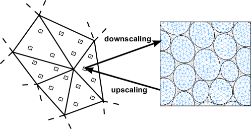
Figure 2: Scale transitions between the macroscale (left) and the mesoscale (right) problems. Downscaling (macro to meso): obtaining proper boundary conditions and the source terms for the mesoscale problem from the current macroscale solution. Upscaling (meso to macro): calculating effective quantities (e.g. material properties) for the macroscale problem from the mesoscale solution

[53].

Additionally, $\text{\text{\bf grad}}{{}_{y}}\,{v_{c}}(\mbox{\boldmath$x$},\cdot,t)=\boldsymbol{e}_{1}(\mbox{\boldmath$x$},\cdot,t)-\partial_{t}\boldsymbol{a}_{c}(\mbox{\boldmath$x$},\cdot,t)$ also belongs to $\boldsymbol{H}_{*}(\text{\bf curl};\mathcal{Y})$, which is automatically ensured by the curl theorem:

(4.16) $$\int_{\Gamma_{m}}\boldsymbol{n}\times\text{\text{\bf grad}}{{}_{y}}\,{v_{c}}\text{d}y=\int_{\Omega_{m}}\text{\text{\bf curl}}{{}_{y}}\,{\text{\text{\bf grad}}{{}_{y}}\,{v_{c}}}\text{d}y.$$

Further we choose a periodic $v_{c}$.

The convergence of the electric current density $\langle\mbox{\boldmath$j$}_{m}\rangle_{\Omega_{mc}}=\mbox{\boldmath$j$}_{M}$ also leads to the following relation:

(4.17) $$\int_{\Omega_{mc}}\mbox{\boldmath$j$}_{c}(\mbox{\boldmath$x$},\mbox{\boldmath$y$},t)\,\textrm{d}y\\ =-\int_{\Omega_{mc}}\sigma\Big{(}\partial_{t}\mbox{\boldmath$a$}_{c}(\mbox{\boldmath$x$},\mbox{\boldmath$y$},t)+\text{\text{\bf grad}}{}\,{v_{c}(\mbox{\boldmath$x$},\mbox{\boldmath$y$},t)}\Big{)}\,\textrm{d}y=\boldsymbol{0},\,\,\forall(\mbox{\boldmath$x$},t)\in\mathbb{R}_{T}^{3}.$$

The upscaling consists in computing the missing constitutive laws $\sigma_{M}$, $\displaystyle\boldsymbol{\mathcal{H}}_{M}$ together with $\partial\boldsymbol{\mathcal{H}}_{M}/\partial\mbox{\boldmath$b$}_{M}$ at the macroscale using the mesoscale fields. Due to the linearity of the electric law, the asymptotic expansion theory can be applied. Therefore, we compute once and for all the homogenized electric conductivity by solving a unique cell problem. A similar approach was also adopted in [12].

The upscaling of the nonlinear magnetic law is performed by averaging the magnetic field (consequence of the two-scale convergence of the magnetic field):

(4.18) $$\mbox{\boldmath$h$}_{M}(\mbox{\boldmath$x$},t)=\boldsymbol{\mathcal{H}}_{M}\left(\mbox{\boldmath$b$}_{M}(\mbox{\boldmath$x$},t)\right)\\ =\dfrac{1}{|\Omega_{mc}|}\int_{\Omega_{mc}}\boldsymbol{\mathcal{H}}\left(\text{\text{\bf curl}}{{}_{x}}\,{\mbox{\boldmath$a$}_{M}(\mbox{\boldmath$x$},t)}+\text{\text{\bf curl}}{{}_{y}}\,{\mbox{\boldmath$a$}_{c}(\mbox{\boldmath$x$},\mbox{\boldmath$y$},t)},\mbox{\boldmath$x$}\right)\textrm{d}y.$$

For the $i$-th Gauß point, the Jacobian expression reads

(4.19) $$\frac{\mathrm{d}\boldsymbol{\mathcal{H}}_{\mathrm{M}}}{\mathrm{d}\mbox{\boldmath$b$}_{\mathrm{M}}}=\frac{1}{|\Omega_{\textrm{m}}|}\int_{\Omega_{\textrm{m}}}\left(\dfrac{\partial\boldsymbol{\mathcal{H}}}{\partial\mbox{\boldmath$b$}_{\mathrm{M}}}+\dfrac{\partial\boldsymbol{\mathcal{H}}}{\partial\mbox{\boldmath$b$}_{\mathrm{c}}}\dfrac{\partial\boldsymbol{\mathcal{B}}_{\mathrm{c}}}{\partial\mbox{\boldmath$b$}_{\mathrm{M}}}\right)\text{d}\mbox{\boldmath$y$}$$

with $\mbox{\boldmath$b$}_{\mathrm{c}}(\mbox{\boldmath$x$},\mbox{\boldmath$y$},t)=\text{\text{\bf curl}}{{}_{y}}\,{\mbox{\boldmath$a$}_{\mathrm{c}}(\mbox{\boldmath$x$},\mbox{\boldmath$y$},t)}=\boldsymbol{\mathcal{B}}_{\mathrm{c}}\left(\mbox{\boldmath$y$},\text{\text{\bf curl}}{{}_{x}}\,{\mbox{\boldmath$a$}_{\mathrm{M}}}(\mbox{\boldmath$x$},t)\right)$ and $\mbox{\boldmath$b$}_{M}=\text{\text{\bf curl}}{{}_{x}}\,{\mbox{\boldmath$a$}_{\mathrm{M}}}$. The derivative w.r.t. the mesoscale vector potential $\mbox{\boldmath$a$}_{\mathrm{M}}$ is given by

(4.20) $$\dfrac{\mathrm{d}\boldsymbol{\mathcal{H}}_{\mathrm{M}}}{\mathrm{d}\mbox{\boldmath$a$}_{\mathrm{M}}}=\dfrac{\mathrm{d}\boldsymbol{\mathcal{H}}_{\mathrm{M}}}{\mathrm{d}\mbox{\boldmath$b$}_{\mathrm{M}}}\dfrac{\mathrm{d}\mbox{\boldmath$b$}_{\mathrm{M}}}{\mathrm{d}\mbox{\boldmath$a$}_{\mathrm{M}}}.$$

The computation (4.19) involves the Fréchet derivative of $\boldsymbol{\mathcal{B}}_{\mathrm{c}}$ with respect to the macroscale magnetic density $\mbox{\boldmath$b$}_{\mathrm{M}}$. This derivative can be evaluated numerically using the finite difference. In [54], several mesoscale problems per Gauß point were solved in parallel. A first problem is solved using (4.11)–(4.12) for the three-dimensional problems (resp. (4.13)–(4.14) for the two-dimensional case) to find the solution when a macroscale source $\boldsymbol{b}_{M}$ is applied. Then, a time and space independent magnetic induction perturbation term $\delta\mbox{\boldmath$b$}_{i}$ oriented along the $i$ directions (${}_{i}=_{x},_{y}$ and _z) is added to the macroscale source terms. Therefore, three (resp. two) additional problems analogous to (4.11)–(4.12) (resp. (4.13)–(4.14) for the two-dimensional case) are solved in order to determine the Jacobian $\mathrm{d}\boldsymbol{\mathcal{H}}_{\mathrm{M}}/\mathrm{d}\mbox{\boldmath$b$}_{\mathrm{M}}$ needed for the Newton-Raphson scheme. The total magnetic induction $\mbox{\boldmath$b$}_{m}$ for these problems are expressed as:

(4.21) $$\mbox{\boldmath$b$}_{m}=\boldsymbol{b}_{M}+\text{\text{\bf curl}}{{}_{y}}\,{\boldsymbol{a}_{c}}+\delta\mbox{\boldmath$b$}_{i}=\text{\text{\bf curl}}{{}_{y}}\,{\left(\boldsymbol{a}_{c}+\kappa(\boldsymbol{b}_{M}\times\mbox{\boldmath$y$})+\kappa(\delta\mbox{\boldmath$b$}_{i}\times\mbox{\boldmath$y$})\right)}=\text{\text{\bf curl}}{{}_{y}}\,{\mbox{\boldmath$a$}_{m}},$$

which can be derived from the total magnetic vector potential:

(4.22) $$\mbox{\boldmath$a$}_{m}=\boldsymbol{a}_{c}-\text{\text{\bf grad}}{{}_{y}}\,{v_{c}}+\kappa(\boldsymbol{b}_{M}\times\mbox{\boldmath$y$})+\kappa(\delta\mbox{\boldmath$b$}_{i}\times\mbox{\boldmath$y$}).$$

These developments allow to transform the three dimensional equation (4.11) into

(4.23) $$\Big{(}\sigma\partial_{t}\mbox{\boldmath$a$}_{c},\mbox{\boldmath$a$}_{c}^{\prime}\Big{)}_{\Omega_{mc}}+\Big{(}\boldsymbol{\mathcal{H}}(\text{\bf curl}_{y}\mbox{\boldmath$a$}_{c}+\mbox{\boldmath$b$}_{M}+\delta\mbox{\boldmath$b$}_{i},\mbox{\boldmath$x$}),\text{\bf curl}_{y}\mbox{\boldmath$a$}_{c}^{\prime}\Big{)}_{\Omega_{m}}+\\ \Big{(}\sigma\text{\bf grad}_{y}v_{c},\mbox{\boldmath$a$}_{c}^{\prime}\Big{)}_{\Omega_{mc}}=\Big{(}\sigma(\mbox{\boldmath$e$}_{M}-\kappa\partial_{t}\mbox{\boldmath$b$}_{M}\times\mbox{\boldmath$y$}),\mbox{\boldmath$a$}_{c}^{\prime}\Big{)}_{\Omega_{mc}}.$$

Notice that the time derivative of the constant term in equation (4.22) disappears. We also modify the two dimensional equation (4.13) as

(4.24) $$\Big{(}\sigma\partial_{t}a_{zc},a_{zc}^{\prime}\Big{)}_{\Omega_{mc}}+\Big{(}\boldsymbol{\mathcal{H}}(\boldsymbol{1}_{z}\times\text{\text{\bf grad}}{{}_{y}}\,{a_{zc}}+\mbox{\boldmath$b$}_{M}+\delta\mbox{\boldmath$b$}_{i},\mbox{\boldmath$x$}),\boldsymbol{1}_{z}\times\text{\text{\bf grad}}{{}_{y}}\,{a_{zc}^{\prime}}\Big{)}_{\Omega_{m}}+\\ \Big{(}\sigma u_{c},a_{zc}^{\prime}\Big{)}_{\Omega_{mc}}=\Big{(}\sigma(\mbox{\boldmath$e$}_{M}-\kappa\partial_{t}\mbox{\boldmath$b$}_{M}\times\mbox{\boldmath$y$}),\boldsymbol{1}_{z}a_{zc}^{\prime}\Big{)}_{\Omega_{mc}}.$$

Equations (4.12) and (4.14) remain unchanged. This leads to the solution $\boldsymbol{h}_{M}+\delta_{\mbox{\boldmath$b$}_{i}}\boldsymbol{h}_{M}$ where $\delta_{\mbox{\boldmath$b$}_{i}}\boldsymbol{h}_{M}$ is the perturbation of the magnetic field in direction $i$. We can therefore compute the elements of the tangent matrix as:

(4.25) $$\left(\dfrac{\partial\boldsymbol{\mathcal{H}}_{M}}{\partial\boldsymbol{b}_{M}}\right)_{ij}\approx\dfrac{(\delta_{\mbox{\boldmath$b$}_{i}}\boldsymbol{h}_{M})_{j}}{\delta\mbox{\boldmath$b$}_{i}}.$$

Further mathematical justifications of the numerical computation of the tangent matrix are given in Section 4.2.

4.2 Finite element implementation

In this section we discuss the numerical implementation of the homogenized problem using the finite element method. The numerical approximation involves errors the sources of which can be numerous in the case of the MQS problem:

• the error due to the the finiteness of the mesoscale domain (instead of $\varepsilon\rightarrow 0$),

• the error due to the modified mesoscale problem (4.6 a-b a-b),

• the error due to scale transitions,

• the error due to the approximation using a finite dimensional space in the Galerkin approximation,

• the error due to Euler’s time stepper,

• the error in the Newton–Raphson scheme used for solving the nonlinear macroscale and the mesoscale problems,

• the error due to the resolution of the linear systems,

• the error in reduced Jacobian,

• the error resulting from the application of the homogenization near the boundaries of the computational domain, etc.

This paper does not deal with the error analysis.

Using a similar approach to the one used in [52], the macroscale and mesoscale equations are solved using the finite element method. The fields $\mbox{\boldmath$a$}_{\mathrm{M}}^{H}$ and $\mbox{\boldmath$a$}_{\mathrm{c}}^{H}$ are approximation of the continuous fields $\mbox{\boldmath$a$}_{\mathrm{M}}$ and $\mbox{\boldmath$a$}_{\mathrm{c}}$ on the discretized computational domain and $\mbox{\boldmath$a$}_{\mathrm{c}}^{H}\in(0,T]\times\mbox{\boldmath$W$}_{H,0}^{\mathrm{M}}$ and $\mbox{\boldmath$a$}_{\mathrm{c}}^{H}\in(0,T]\times\mbox{\boldmath$W$}_{h,0}^{\mathrm{m}}$ where $\times\mbox{\boldmath$W$}_{H,0}^{\mathrm{M}}$ and $\mbox{\boldmath$W$}_{h,0}^{\mathrm{m}}$ are discrete subspaces of $\boldsymbol{H}_{e}^{0}(\text{\bf curl};\Omega)$ and $\boldsymbol{H}_{e}^{0}(\text{\bf curl};\Omega_{m})$

(4.26) $$\mbox{\boldmath$a$}_{\mathrm{M}}(\mbox{\boldmath$x$},t)\approx\mbox{\boldmath$a$}_{\mathrm{M}}^{H}(\mbox{\boldmath$x$},t)=\sum_{p=1}^{N_{\mathrm{M}}}\mbox{$\alpha$}_{\textrm{M},p}(t)\mbox{\boldmath$a$}^{\prime}_{\textrm{M},p}(\mbox{\boldmath$x$})\\ \qquad\textrm{and}\qquad\mbox{\boldmath$a$}_{\mathrm{c}}^{(i)}(\mbox{\boldmath$y$},t)\approx\mbox{\boldmath$a$}_{\mathrm{c}}^{H}(\mbox{\boldmath$y$},t)=\sum_{p=1}^{N_{\mathrm{c}}}\mbox{$\alpha$}_{\textrm{c},p}^{(i)}(t)\mbox{\boldmath$a$}^{\prime}_{\textrm{c},p}(\mbox{\boldmath$y$}),$$

where the superscript $i=1,2,\cdots,N_{\textrm{GP}}$ refers to the enumeration of mesoscale problems, $N_{\mathrm{M}}$ and $N_{\mathrm{c}}$ are the number of degrees of freedom for discretized fields at the macroscale and the mesoscale, respectively. Space discretization leads to the semidiscrete coupled problem:

Find waveforms $[\mbox{\boldmath$\alpha$}_{\mathrm{M}}(t),\mbox{\boldmath$\alpha$}_{\mathrm{c}}^{(1)}(t),\ldots,\mbox{\boldmath$\alpha$}_{\mathrm{c}}^{(N_{\mathrm{GP}})}(t)]$ such that

(4.27) $$\mbox{\boldmath$M$}_{\mathrm{M}}\partial_{t}\mbox{\boldmath$\alpha$}_{\mathrm{M}}+\boldsymbol{\mathcal{F}}_{\mathrm{M}}(\mbox{\boldmath$\alpha$}_{\mathrm{M}},\mbox{\boldmath$\alpha$}_{\mathrm{c}})=0,$$

and for the mesoscale problems $i=1,\ldots,N_{\mathrm{GP}}$

(4.28) $$\mbox{\boldmath$M$}_{\mathrm{m}}\partial_{t}\mbox{\boldmath$\alpha$}_{\mathrm{c}}^{(i)}+\boldsymbol{\mathcal{F}}_{\mathrm{m}}(\mbox{\boldmath$\alpha$}_{\mathrm{c}}^{(i)},\mbox{\boldmath$\alpha$}_{\mathrm{M}}^{(i)},\partial_{t}\mbox{\boldmath$\alpha$}_{\mathrm{M}}^{(i)})=0$$

for a given set of initial values $[\mbox{\boldmath$\alpha$}_{\mathrm{M}}(t_{0}),\mbox{\boldmath$\alpha$}_{\mathrm{c}}^{(1)}(t_{0}),\ldots,\mbox{\boldmath$\alpha$}_{\mathrm{c}}^{(N_{\mathrm{GP}})}(t_{0})]$. where $\mbox{\boldmath$M$}_{\mathrm{M}}:=\Big{(}\sigma_{\mathrm{M}}\mbox{\boldmath$a$}_{\mathrm{M}},\mbox{\boldmath$a$}_{\mathrm{M}}^{\prime}\Big{)}_{\Omega_{\mathrm{c}}}$ with $\mbox{\boldmath$a$}_{\mathrm{M}}$ and $\mbox{\boldmath$a$}_{\mathrm{M}}^{\prime}$, the ansatz functions, the functions $\boldsymbol{\mathcal{F}}_{\mathrm{M}}(\cdots)$ and $\boldsymbol{\mathcal{F}}_{\mathrm{m}}(\cdots)$ are the semi-discreet terms involving the nonlinear magnetic terms stemming from (4.3) and (4.11) by inserting (4.26).

The time discretization using an implicit Euler method followed by the use of the Newton–Raphson method to solve the resulting nonlinear problem leads the following Jacobian

(4.29) $$J_{\boldsymbol{\mathcal{R}}}^{(j,k)}:=\frac{1}{\Delta t_{k}}\begin{pmatrix}\displaystyle{\mbox{\boldmath$M$}_{\mathrm{M}}\vphantom{\frac{\partial\boldsymbol{\mathcal{F}}^{(j,k)}_{\mathrm{M}}}{\partial\mbox{\boldmath$\alpha$}_{\mathrm{M}}^{(j,k)}}}}&\displaystyle{0}&\displaystyle{\cdots}&\displaystyle{0}\\ \displaystyle{0}&\displaystyle{\mbox{\boldmath$M$}_{\mathrm{m}}\vphantom{\frac{\partial\boldsymbol{\mathcal{F}}^{(j,k)}_{\mathrm{M}}}{\partial\mbox{\boldmath$\alpha$}_{\mathrm{M}}^{(j,k)}}}}&\displaystyle{0}&\displaystyle{0}\\ \displaystyle{\vdots}&0&\displaystyle{\ddots}&0\\ \displaystyle{0}&0&0&\displaystyle{\mbox{\boldmath$M$}_{\mathrm{m}}\vphantom{\frac{\partial\boldsymbol{\mathcal{F}}^{(j,k)}_{\mathrm{M}}}{\partial\mbox{\boldmath$\alpha$}_{\mathrm{M}}^{(j,k)}}}}\end{pmatrix}+\\ \begin{pmatrix}\displaystyle{\frac{\partial\boldsymbol{\mathcal{F}}^{(j,k)}_{\mathrm{M}}}{\partial\mbox{\boldmath$\alpha$}_{\mathrm{M}}^{(j,k)}}}&\displaystyle{\frac{\partial\boldsymbol{\mathcal{F}}^{(j,k)}_{\mathrm{M}}}{\partial\mbox{\boldmath$\alpha$}_{\mathrm{c}}^{(1,j,k)}}}&\displaystyle{\cdots}&\displaystyle{\frac{\partial\boldsymbol{\mathcal{F}}^{(j,k)}_{\mathrm{M}}}{\partial\mbox{\boldmath$\alpha$}_{\mathrm{c}}^{(N_{\mathrm{GP}},j,k)}}}\\ \displaystyle{\frac{\partial\boldsymbol{\mathcal{F}}^{(1,j,k)}_{\mathrm{m}}}{\partial\mbox{\boldmath$\alpha$}_{\mathrm{M}}^{(1,j,k)}}}&\displaystyle{\frac{\partial\boldsymbol{\mathcal{F}}^{(1,j,k)}_{\mathrm{m}}}{\partial\mbox{\boldmath$\alpha$}_{\mathrm{c}}^{(1,j,k)}}}&\displaystyle{0}&\displaystyle{0}\\ \displaystyle{\vdots}&0&\displaystyle{\ddots}&0\\ \displaystyle{\frac{\partial\boldsymbol{\mathcal{F}}^{(N_{\mathrm{GP}},j,k)}_{\mathrm{m}}}{\partial\mbox{\boldmath$\alpha$}_{\mathrm{M}}^{(N_{\mathrm{GP}},j,k)}}}&0&0&\displaystyle{\frac{\partial\boldsymbol{\mathcal{F}}^{(N_{\mathrm{GP}},j,k)}_{\mathrm{m}}}{\partial\mbox{\boldmath$\alpha$}_{\mathrm{c}}^{(N_{\mathrm{GP}},j,k)}}}\end{pmatrix}$$

where $\mbox{\boldmath$\alpha$}_{\mathrm{M}}^{(j,k)}$ and $\mbox{\boldmath$\alpha$}_{\mathrm{c}}^{(i,j,k)}$ denote the $j^{\mathrm{th}}$ Newton–Raphson iterates and

(4.30) $$\boldsymbol{\mathcal{F}}_{\mathrm{M}}^{(j,k)}:=\boldsymbol{\mathcal{F}}_{\mathrm{M}}\Big{(}\mbox{\boldmath$\alpha$}_{\mathrm{M}}^{(j,k)},\mbox{\boldmath$\alpha$}_{\mathrm{c}}^{(j,k)}\Big{)}\\ \boldsymbol{\mathcal{F}}_{\mathrm{m}}^{(i,j,k)}:=\boldsymbol{\mathcal{F}}_{\mathrm{m}}\left(\mbox{\boldmath$\alpha$}_{\mathrm{c}}^{(i,j,k)},\mbox{\boldmath$\alpha$}_{\mathrm{M}}^{(i,j,k)},\frac{\mbox{\boldmath$\alpha$}_{\mathrm{M}}^{(i,j,k)}-\mbox{\boldmath$\alpha$}_{\mathrm{M}}^{(i,j,k-1)}}{\Delta t_{k}}\right).$$

where the superscripts $k$ and $j$ are used for time steps and the Newton–Raphson iterations. See [52, Section 4] for more details on the derivation of the Jacobian (4.29). In practice, one does not solve the system above but the Schur complement system with the reduced Jacobian defined by

(4.31) $$\bar{J}_{\boldsymbol{\mathcal{R}}}^{(j,k)}:=\frac{\mbox{\boldmath$M$}_{\mathrm{M}}}{\Delta t_{k}}+\dfrac{\partial\boldsymbol{\mathcal{F}}^{(j,k)}_{\mathrm{M}}}{\partial\mbox{\boldmath$\alpha$}_{\mathrm{M}}^{(j,k)}}-\sum_{i=1}^{N_{\mathrm{GP}}}\left(\dfrac{\partial\boldsymbol{\mathcal{F}}^{(j,k)}_{\mathrm{M}}}{\partial\mbox{\boldmath$\alpha$}_{\mathrm{c}}^{(i,j,k)}}\Big{(}\frac{\mbox{\boldmath$M$}_{\mathrm{m}}}{\Delta t_{k}}+\dfrac{\partial\boldsymbol{\mathcal{F}}^{(i,j,k)}_{\mathrm{m}}}{\partial\mbox{\boldmath$\alpha$}_{\mathrm{c}}^{(i,j,k)}}\Big{)}^{-1}\,\dfrac{\partial\boldsymbol{\mathcal{F}}^{(i,j,k)}_{\mathrm{m}}}{\partial\mbox{\boldmath$\alpha$}_{\mathrm{M}}^{(i,j,k)}}\right).$$

Algorithm 1 Pseudocode for the monolithic FE-HMM

macroscale source $\mbox{\boldmath$j$}_{\mathrm{s}}$ and mesh.

macroscale fields, mesoscale fields and global quantities.

procedure macroscale problem

     $t\leftarrow t_{0}$, initialize the macroscale field $\mbox{\boldmath$a$}_{\mathrm{M}}|_{t_{0}}=\mbox{\boldmath$a$}_{\mathrm{M}0}$,

     for $(k\leftarrow 1$ To $N_{\mathrm{TS}})$ do $\triangleright$ the macroscale time loop $($index $k$$)$

         for $(j\leftarrow 1$ To $N_{\mathrm{NR}}^{\mathrm{M}})$ do $\triangleright$ the macroscale NR loop $($index $j$$)$

              for $(i\leftarrow 1$ To $N_{\mathrm{GP}})$ do $\triangleright$ parallel solutions of meso-problems $($index $i$$)$

                  downscale the macroscale sources,

                  compute the mesoscale fields, see Algorithm 2,

                  compute and upscale the homogenized law $\boldsymbol{\mathcal{H}}_{\mathrm{M}}$ and

                  $\partial\boldsymbol{\mathcal{H}}_{\mathrm{M}}/\partial\mbox{\boldmath$b$}_{\mathrm{M}}$

              end for

              assemble the Jacobian $\bar{J}_{\boldsymbol{\mathcal{R}}}^{(j,k)}$ from (4.31) to solve the macroscale problem,

         end for

     end for

end procedure

Algorithm 2 Pseudocode for one mesoscale problem

macroscale sources and the mesoscale mesh.

homogenized law $\boldsymbol{\mathcal{H}}_{\mathrm{M}}$ and $\partial\boldsymbol{\mathcal{H}}_{\mathrm{M}}/\partial\mbox{\boldmath$b$}_{\mathrm{M}}$, per Gauß  point for $N_{m}$ problems.

procedure mesoscale problem

     prescribe periodic boundary conditions, impose sources,

     $t\leftarrow t_{\mathrm{M}}$, initialize the correction term $\mbox{\boldmath$a$}_{\mathrm{c}}|_{t_{\mathrm{M}}}$

     for $(p\leftarrow 1$ To $N^{\mathrm{m}}_{\mathrm{dim}})$ do $\triangleright$ solve $N^{\mathrm{m}}_{\mathrm{dim}}$ mesoscale problems for the $k^{th}$ time step

         for $(j\leftarrow 1$ To $N_{\mathrm{NR}}^{\mathrm{m}})$ do $\triangleright$ the mesoscale NR loop $($index $j$$)$

              assemble the matrix and solve the mesoscale problem.

         end for

     end for

end procedure

The overall FE-HMM method is described in Algorithm 1 and Algorithm 2. It starts with the initialization of the macroscale problem followed by a time loop. For each time step, a nonlinear system is solved using the Newton–Raphson method until convergence (i.e. the residual $res_{\textrm{M}}$ is smaller than some prescribed tolerance $tol_{\textrm{M}}$). Therefore, $N_{\mathrm{GP}}$ mesoscale problems are solved in parallel and the homogenized law are obtained. The term $\Big{(}\frac{\mbox{\boldmath$M$}_{\mathrm{m}}}{\Delta t_{k}}+\partial\boldsymbol{\mathcal{F}}^{(i,j,k)}_{\mathrm{m}}/\partial\mbox{\boldmath$\alpha$}_{\mathrm{c}}^{(i,j,k)}\Big{)}^{-1}\,\Big{(}\partial\boldsymbol{\mathcal{F}}^{(i,j,k)}_{\mathrm{m}}/\partial\mbox{\boldmath$\alpha$}_{\mathrm{M}}^{(i,j,k)}\Big{)}$ in (4.31) can be interpreted as the discretization of the Fréchet derivative $\Big{(}\partial\boldsymbol{\mathcal{B}}^{(i)}_{\mathrm{c}}/\partial\mbox{\boldmath$b$}_{\mathrm{M}}\Big{)}$ in (4.19) (see [52]).

4.3 The static case

The static problem can be seen as a simplified version of the dynamic problem obtained by neglecting the time derivatives. The macroscale weak formulation is derived from the $\mbox{\boldmath$a$}-v$ formulation described in the section 4.1.1. The three-dimensional macroscale weak formulation reads: find $\mbox{\boldmath$a$}_{M}\in\boldsymbol{H}_{e}(\text{\bf curl};\Omega)$ such that

(4.32) $$\left(\mbox{\boldmath$h$}_{M},\text{\text{\bf curl}}{{}_{x}}\,{\mbox{\boldmath$a$}_{M}^{\prime}}\right)_{\Omega}=-\left<\boldsymbol{n}\times\boldsymbol{h}_{M},\boldsymbol{a}_{M}^{\prime}\right>_{\Gamma_{h}}+\left(\mbox{\boldmath$j$}_{s},\mbox{\boldmath$a$}_{M}^{\prime}\right)_{\Omega_{s}}$$

holds for all test functions $\mbox{\boldmath$a$}_{M}^{\prime}\in\boldsymbol{H}_{e}^{0}(\text{\bf curl};\Omega)$. The two-dimensional macroscale problem reads: find $a_{zM}\in H_{e}^{1}(\Omega)$ such that

(4.33) $$\left(\mbox{\boldmath$h$}_{M},\boldsymbol{1}_{z}\times\text{\text{\bf grad}}{{}_{x}}\,{a_{zM}^{\prime}}\right)_{\Omega}\\ =-\langle{\boldsymbol{n}}\times{\boldsymbol{h}_{M}},a_{zM}^{\prime}\boldsymbol{1}_{z}\rangle_{\Gamma_{h}}+\left(j_{s},a_{zM}^{\prime}\right)_{\Omega_{s}}\,,\qquad\forall a_{zM}^{\prime}\in H_{e}^{10}(\Omega).$$

The three-dimensional mesoscale problem can be derived from (4.11): find $\mbox{\boldmath$a$}_{c}\in\boldsymbol{H}_{*}(\text{\bf curl};\mathcal{Y})$ such that

(4.34) $$\left(\boldsymbol{\mathcal{H}}(\text{\bf curl}_{y}\mbox{\boldmath$a$}_{c}+\mbox{\boldmath$b$}_{M},\mbox{\boldmath$x$},\mbox{\boldmath$y$}),\text{\bf curl}_{y}\mbox{\boldmath$a$}_{c}^{\prime}\right)_{\Omega_{m}}=0\,,\qquad\forall\mbox{\boldmath$a$}_{c}^{\prime}\in\boldsymbol{H}_{*}(\text{\bf curl};\mathcal{Y})$$

and the two-dimensional mesoscale formulation reads: find $a_{zc}\in H^{1}_{*}(\mathcal{Y})$ such that

(4.35) $$\left(\boldsymbol{\mathcal{H}}(\boldsymbol{1}_{z}\times\text{\text{\bf grad}}{{}_{y}}\,{a_{zc}}+\mbox{\boldmath$b$}_{M},\mbox{\boldmath$x$},\mbox{\boldmath$y$}),\boldsymbol{1}_{z}\times\text{\text{\bf grad}}{{}_{y}}\,{a_{zc}^{\prime}}\right)_{\Omega_{m}}=0\,,\qquad\forall a_{zc}^{\prime}\in H^{1}_{*}(\mathcal{Y}).$$

5 Numerical tests

The models developed in the previous section are valid for the general three-dimensional problems. In this section we apply the models to solve nonlinear two-dimensional eddy current problem involving nonlinear/hysteretic materials using Problems 4.2 and 4.4.

5.1 Description of the problem

We consider a soft magnetic composite (SMC) material to test the ideas developed in the previous sections. An idealized 2D periodic SMC (with $20\,\times\,20$ grains) surrounded by an inductor is studied. We solve this academic problem using the SMC structure depicted in Figure 3 (only $10\,\times\,10$ grains are shown).

Figure 3: Two-dimensional soft magnetic composite geometry (only 100 grains out of the actual 400 are drawn). Top and bottom inductors carry opposite source currents. The dimensions are $L=1000\,\mu$m, $e_{a}=150\,\sqrt{2}/2\,\mu$m, $e_{i}=100\,\mu$m and $e_{gap}=100\,\mu$m.

Figure 4: Geometry used for computations (one fourth taking advantage of symmetries). Left: Reference geometry (only 25 grains out of the actual 100 are depicted). Right: Homogenized geometry.

The source current $\mbox{\boldmath$j$}_{s}$ is imposed perpendicular to the $xy$-plane $\mbox{\boldmath$j$}_{s}=(0,0,j_{s})$ with $j_{s}=j_{s0}s(t)$ where $j_{s0}$ is the amplitude and $s(t)=\sin(2\pi ft)$. Therefore, the problem can be solved using a two-dimensional magnetic vector potential formulation with $\mbox{\boldmath$a$}=(0,0,a_{z})$, thus constraining the magnetic flux density $b$ in the $xy$-plane. Only one fourth the structure is considered for numerical computations thanks to the symmetry (see Figure 4 – Left for the reference geometry and Figure 4 – Right for the homogenized geometry). In both cases, the following boundary conditions are imposed on $\Gamma_{\mathrm{inf}},\Gamma_{h}$ and $\Gamma_{v}$:

(5.1) $$(\mbox{\boldmath$n$}\cdot\mbox{\boldmath$b$})|_{\Gamma_{\mathrm{inf}}}=0 \quad\Leftarrow\quad(\mbox{\boldmath$n$}\times\mbox{\boldmath$a$})|_{\Gamma_{\mathrm{inf}}}=\boldsymbol{0},$$

(5.2) $$(\mbox{\boldmath$n$}\cdot\mbox{\boldmath$b$})|_{\Gamma_{\mathrm{h}}}=0 \quad\Leftarrow\quad(\mbox{\boldmath$n$}\times\mbox{\boldmath$a$})|_{\Gamma_{\mathrm{h}}}=\boldsymbol{0},\quad(\mbox{\boldmath$n$}\times\mbox{\boldmath$h$})|_{\Gamma_{\mathrm{v}}}=\boldsymbol{0}.$$

We consider operating frequencies smaller than 50 kHz, which corresponds to $\lambda_{f}\text{ and }\lambda_{M}\simeq\lambda=6000$m). The smallest wavelength of the source is much larger than the length of the structure ($\simeq 500\mu m$) so that the assumption of a magnetoquasistatic problem can be made.

All materials are isotropic, so that the magnetic field $h$ has only $xy$ components. The conducting grains (electric conductivity $\sigma=5\,10^{6}$ S/m) are surrounded by a perfect insulator, linear and non-magnetic ($\mu_{r}=1$). The grains are governed by the following magnetic laws:

1. a nonlinear exponential law $\boldsymbol{\mathcal{H}}(\mbox{\boldmath$b$})=\left(\alpha+\beta\,\exp(\gamma||\mbox{\boldmath$b$}||^{2})\right)\,\mbox{\boldmath$b$}$ with $\alpha=388,\beta=0.3774$ and $\gamma=2.97$ [23].

2. a Jiles–Atherton hysteresis model with parameters $\boldsymbol{\mathcal{M}}_{s}=1,145,500$ A/m, $a=59$ A/m, $k=99$ A/m, $c=0.55$ and $\alpha=1.3\,10^{-4}$ (see [37, 6] for more details on the Jiles–Atherton model and the meaning of the parameters it uses).

Results obtained using the computational homogenization (subscript “comp” for computational homogenization, subscript “M” for Macro and “m” for meso) are compared to the reference results (subscript “Ref”) obtained solving the reference problem (i.e. the weak form of (2.28 a-b a-b)–(2.29 a-b a-b) on a very fine mesh.

Some quantities of interest (global quantities and errors) are defined and used for numerical validation. The global quantities are the reference and the computational homogenization eddy currents losses:

(5.3) $$\tau\textrm{P}_{\mathrm{Ref}}(t)=\int_{\Omega_{c}}(\sigma|\partial_{t}\mbox{\boldmath$a$}^{\varepsilon}(\mbox{\boldmath$x$},t)|^{2})\,\mathrm{d}x,$$

$$\tau\textrm{P}_{\mathrm{m}}(t)=\int_{\Omega}\tau\textrm{P}_{\mathrm{m}}^{\mathrm{up}}(\mbox{\boldmath$x$},t)\,\mathrm{d}x=\int_{\Omega}\Big{(}\frac{1}{|\Omega_{m}|}\int_{\Omega_{\mathrm{mc}}}(\sigma|\partial_{t}\mbox{\boldmath$a$}_{\mathrm{m}}(\mbox{\boldmath$x$},\mbox{\boldmath$y$},t)|^{2})\,\mathrm{d}y\Big{)}\,\mathrm{d}x.$$

The equivalent quantities in terms of the magnetic energy can be defined.

Two types of errors are defined as:

• the relative error in terms of the eddy current losses:

  (5.4) $$\mathrm{Err}_{\tau\textrm{P}}=\dfrac{\parallel\tau\textrm{P}_{\mathrm{m}}-\tau\textrm{P}_{\mathrm{Ref}}\parallel_{L^{\infty}(0,\,T)}}{\parallel\tau\textrm{P}_{\mathrm{Ref}}\parallel_{L^{\infty}(0,\,T)}},$$

• the pointwise relative error on the fields $\mbox{\boldmath$b$}_{\mathrm{M}}$ and $\mbox{\boldmath$b$}_{\mathrm{m}}$:

  (5.5) $$\mathrm{Err}_{\mathrm{M}}^{\mbox{\boldmath$b$}}(\mbox{\boldmath$x$})=\dfrac{\parallel\mbox{\boldmath$b$}_{\mathrm{M}}(\mbox{\boldmath$x$})-\mbox{\boldmath$b$}_{\mathrm{Ref}}(\mbox{\boldmath$x$})\parallel_{L^{2}(0,\,T)}}{\parallel\mbox{\boldmath$b$}_{\mathrm{Ref}}(\mbox{\boldmath$x$})\parallel_{L^{2}(0,\,T)}},\,\\ \mathrm{Err}_{\mathrm{m}}^{\mbox{\boldmath$b$}}(\mbox{\boldmath$x$})=\dfrac{\parallel\mbox{\boldmath$b$}_{\mathrm{m}}(\mbox{\boldmath$x$})-\mbox{\boldmath$b$}_{\mathrm{Ref}}(\mbox{\boldmath$x$})\parallel_{L^{2}(0,\,T)}}{\parallel\mbox{\boldmath$b$}_{\mathrm{Ref}}(\mbox{\boldmath$x$})\parallel_{L^{2}(0,\,T)}},$$

5.2 Results

Results of the reference and the multiscale problems are compared in this section. The latter are obtained by solving a finite element problem on the entire, finely meshed multiscale domain (110,282 triangular elements). Computational results are carried out on a macroscale, coarse mesh (42 quad elements). Mesoscale problems are solved around each numerical quadrature point of the macroscale mesh using a fine mesh (4125 triangular elements).

Figure 5: Terms contributing to the total mesoscale magnetic vector potential for a cell problem centered at ($325,25,0.0$)$\mu m$. Top: the $z$-component of the projection term $\mbox{\boldmath$a$}_{proj}(\mbox{\boldmath$x$},\mbox{\boldmath$y$},t)=\mbox{\boldmath$a$}_{M}(\mbox{\boldmath$x$},t)+\kappa(\mbox{\boldmath$y$}\times\mbox{\boldmath$b$}_{M}(\mbox{\boldmath$x$},t))$. Middle: the $z$-component of the correction term $\mbox{\boldmath$a$}_{c}(\mbox{\boldmath$x$},\mbox{\boldmath$y$},t)$. Bottom: the $z$-component of the total mesoscale vector potential $\mbox{\boldmath$a$}_{tot}(\mbox{\boldmath$x$},\mbox{\boldmath$y$},t)$ {nonlinear case with $j_{s0}=35\times 10^{7}\text{A/m}^{2},f=25\text{ kHz}$}.

Figure 5 depicts the different contributing terms involved in the resolution of the mesoscale problem. The projection term which varies linearly on the mesoscale domain is computed from the macroscale fields as $\mbox{\boldmath$a$}_{proj}(\mbox{\boldmath$x$},\mbox{\boldmath$y$},t)=\mbox{\boldmath$a$}_{M}(\mbox{\boldmath$x$},t)+\kappa(\mbox{\boldmath$y$}\times\mbox{\boldmath$b$}_{M}(\mbox{\boldmath$x$},t))$. This term is then used as a source for the computation of the correction term $\mbox{\boldmath$a$}_{c}(\mbox{\boldmath$x$},\mbox{\boldmath$y$},t)$ at the mesoscale level which allows to derive the total magnetic vector potential $\mbox{\boldmath$a$}_{tot}(\mbox{\boldmath$x$},\mbox{\boldmath$y$},t)=\mbox{\boldmath$a$}_{c}(\mbox{\boldmath$x$},\mbox{\boldmath$y$},t)+\mbox{\boldmath$a$}_{M}(\mbox{\boldmath$x$},t)+\kappa(\mbox{\boldmath$y$}\times\mbox{\boldmath$b$}_{M}(\mbox{\boldmath$x$},t))$.

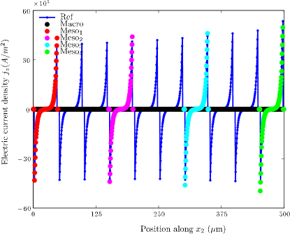
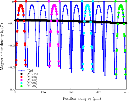
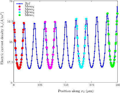
Figure 6: SMC problem, $\boldsymbol{b}$-conform formulations, hysteretic case. Spatial cuts of the $z$-component of the eddy currents $\boldsymbol{j}$ (top), of the $x$-component of the magnetic induction $\boldsymbol{b}$ (middle) and of the magnetic field $\boldsymbol{h}$ (bottom) along the line {$x=25,z=0$} $\mu$m. ($f=10$ kHz, $t=5\,10^{-7}$s for the curve of eddy currents and $t=25\,10^{-7}$s for the curve of the magnetic induction).

The spatial cuts of the magnetic induction $b$, the eddy currents $j$ and the magnetic field $bh$ are shown in Figure 6. The agreement between the reference solution and the mesoscale solution on a cell around certain Gauß  points in the computational domain proves excellent. As expected, small discrepancies are observed near the boundary of the domain (see Tables 2 and 3).

Table 2 displays the values of $\parallel\mbox{\boldmath$b$}\parallel$ obtained from the reference solution (Reference), the macroscale solution (Macro) and the mesoscale solution (Meso) and the corresponding relative pointwise errors (Error meso, Error macro) for $t=6\cdot 10^{-6}$ s. In this table, we observe that the mesoscale error increases with the proximity to the boundary of the computational domain. In the bulk, the error is around 1% and rises up to 14% at the boundary. Indeed, cells located near the boundary do not respect the periodicity assumption, they are not immersed in a periodic environment. The macroscale error is huge and almost independent of the location of the considered point.

Table 2: Soft magnetic composite problem – $\boldsymbol{b}$-conform formulations. Comparison of the reference and the computational (macroscale and mesoscale) magnetic flux density ($\|\boldsymbol{b}\|$ [T]) at different points of the macroscale domain {$t=6\cdot 10^{-6}$ s}.

Position ($\mu$m)	Reference	Meso	Macro	$\mathrm{Err}_{\mathrm{m}}^{\mbox{\boldmath$b$}}(\mbox{\boldmath$x$})(\%)$	$\mathrm{Err}_{\mathrm{M}}^{\mbox{\boldmath$b$}}(\mbox{\boldmath$x$})(\%)$
$(25,25,0)$	0.0157652	0.0158937	0.0347775	0.82	120.60
$(25,475,0)$	0.0186482	0.0181317	0.0403767	2.77	116.52
$(175,175,0)$	0.0158077	0.0158738	0.0346577	0.42	119.25
$(475,25,0)$	0.0156693	0.0158615	0.0345838	1.23	120.70
$(475,475,0)$	0.0184396	0.0158563	0.0417285	14.01	126.30

Table 3 provides the relative $L^{2}(0,T)$ error defined by (5.5). Results of Table 3 allow us to draw the same conclusions as those from Table 2, i.e. the error increases as the point gets closer to the boundary of the computational domain.

Table 3: Soft magnetic composite problem – $\boldsymbol{b}$-conform formulations. Relative $L^{2}(0,T)$ errors of the mesoscale and the macroscale magnetic flux density with regard to the reference, $\mathrm{Err}_{\mathrm{m}}^{\mbox{\boldmath$b$}}(\mbox{\boldmath$x$})$ and $\mathrm{Err}_{\mathrm{M}}^{\mbox{\boldmath$b$}}(\mbox{\boldmath$x$})$, respectively, at different points of the computational domain.

Position ($\mu m$)	$\mathrm{Err}_{\mathrm{m}}^{\mbox{\boldmath$b$}}(\mbox{\boldmath$x$})(\%)$	$\mathrm{Err}_{\mathrm{M}}^{\mbox{\boldmath$b$}}(\mbox{\boldmath$x$})(\%)$
$(25,25,0)$	3.27	11.49
$(25,475,0)$	4.93	15.13
$(175,175,0)$	3.01	11.88
$(475,25,0)$	3.04	12.27
$(475,475,0)$	15.46	22.91

Figure 7: SMC problem, $\boldsymbol{b}$-conform formulations, hysteretic case. Instantaneous Joule losses and absolute error between the reference (Ref) and the computational (Comp) solutions. Hysteretic case. Left: $f=50$ Hz. Right: $f=2500$ Hz.

Figure 7 depicts the evolution of the eddy currents losses for excitations at $50$ Hz and $2500$ Hz (which correspond to the case with enhanced skin effect). A good agreement between Joules losses is observed for both frequencies: a maximum error of $1.41\,\%$ and $6.69\,\%$ are observed for $f=50$ Hz and $f=2500$ Hz, respectively.

Table 4 contains the relative $L^{\infty}(0,T)$ error of the Joule losses defined by equation (5.4) as a function of frequency.

Table 4: Soft magnetic composite problem – $\boldsymbol{b}$-conform formulations. Relative $L^{\infty}(0,T)$ norm error on the total Joule losses as a function of the frequency.

Frequency (Hz)	$\mathrm{Err}_{\tau\textrm{P}}$ ($\%$)
$50$	$1.41$
$100$	$1.46$
$250$	$1.61$
$1000$	$3.42$
$2500$	$6.69$

Figure 8 shows the convergence of the residual resulting from the resolution by the Newton–Raphson method as a function of the number of nonlinear iteration. It can be seen that the macroscale problem converges quadratically while the mesoscale problems converge at an average rate of 1.33.

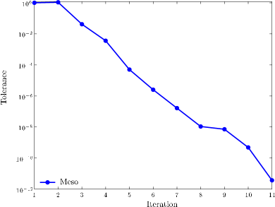
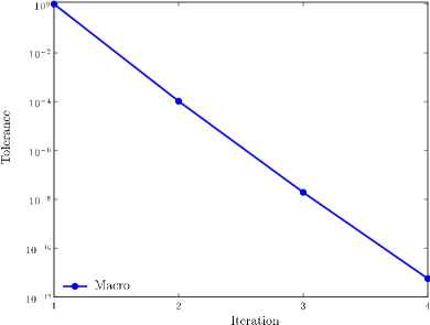
Figure 8: SMC problem, $\boldsymbol{b}$-conform formulations, hysteretic case. Convergence of the error as a function of nonlinear iterations. Top: mesoscale problem. Bottom: macroscale problem.

6 Conclusions

In this paper we have developed a computational multiscale method inspired by the HMM approach to solve nonlinear, possibly hysteretic magnetoquasistatic problems on multiscale domains (e.g. composite materials, lamination stacks, etc.). To construct the computational multiscale model, we combine theoretical results from two-scale convergence theory and asymptotic homogenization. The two-scale convergence and periodic unfolding methods are used for deriving the partial differential equations governing fields at both the macroscale and the mesoscale levels, valid in the nonlinear regime and in the presence of curl differential operators. Asymptotic homogenization is used for defining a mesoscale problem in the case of linear constitutive laws (e.g. the linear electric conductivity law).

Although the theoretical foundation is only valid in the case of linear and nonlinear problems governed by a maximal monotone operator, in practice, the resulting numerical multiscale scheme has been successfully applied to general magnetoquasistatic problems also exhibiting memory effects (hysteresis). The numerical tests were performed for magnetodynamic problems, using $b$-conform formulations. An excellent agreement has been obtained between the reference solutions (computed using a brute force approach) and the computational (mesoscale) solutions. We observed larger errors near the boundary of the computational domain as the cell problems defined near the boundary are not immersed in a periodic environment. The eddy current losses are also accurately evaluated. The error on these losses increases as a function of the frequency.

For the considered academic test case, the proposed computational multiscale method fulfills the original goals (Section 1): it allows to solve multiscale magnetoquasistatic problems, including the computation of local fields at the mesoscale and the accurate evaluation of electromagnetic losses. It naturally handles nonlinear or hysteretic materials and periodic mesoscale geometries. From an engineering point of view, the approach could be straightforwadly applied to deal with more complex multiscale geometries.

The main disadvantage of the method is its higher computational cost. However, since all the mesoscale problems are independent, the method is perfectly suited for modern massively parallel computers, and we thus believe that it has a lot of potential, even compared to brute force approaches, which do not scale well.

References

• [1] A. Abdulle, The finite element heterogeneous multiscale method: a computational strategy for multiscale PDEs, GAKUTO International Series Math. Sci. Appl., Multiple scales problems in Biomathematics, Mechanics, Physics and Numerics, 31 (2009), pp. 133–181.
• [2] A. Abdulle and W. E, Finite difference heterogeneous multi-scale method for homogenization problems, Journal of Computational Physics, 191 (2003), pp. 18–39, doi:10.1016/S0021-9991(03)00303-6.
• [3] R. Acevedo and G. Loaiza, A fully-discrete finite element approximation for the eddy currents problem, Ingeniería y Ciencia, 9 (2013), pp. 111–145.
• [4] F. Bachinger, U. Langer, and J. Schöberl, Numerical analysis of nonlinear multiharmonic eddy current problems, Numerische Mathematik, 100 (2005), pp. 593–616.
• [5] M. Belkadi, B. Ramdane, D. Trichet, and J. Fouladgar, Non linear homogenization for calculation of electromagnetic properties of soft magnetic composite materials, IEEE: Transaction on Magnetics, 45 (2009), pp. 4317–4320.
• [6] A. Benabou, S. Clénet, and F. Piriou, Comparison of Preisach and Jiles-Atherton models to take into account hysteresis phenomenon for finite element analysis, Journal of Magnetism and Magnetic Materials, 261 (2003), pp. 305–310.
• [7] A. Bensoussan, J.-L. Lions, and G. Papanicolaou, Asymptotic Analysis for Periodic Structures, American Mathematical Society, 2011.
• [8] A. Bossavit, Électromagnétisme, en vue de la modélisation, Springer-Verlag, 1993.
• [9] A. Bossavit, Effective penetration depth in spatially periodic grids: a novel approach to homogenization, in Proceedings, 1994, pp. 859–864.
• [10] A. Bossavit, Homogenizing spatially periodic materials with respect to maxwell equations: Chiral materials by mixing simple ones, in Proceedings, 1996, pp. 564–567.
• [11] A. Bossavit, Computational Electromagnetism. Variational Formulations, Edge Elements, Complementarity, Academic Press, 1998.
• [12] O. Bottauscio, V. Chiado Piat, M. Chiampi, M. Codegone, and A. Manzin, Nonlinear homogenization technique for saturable soft magnetic composites, IEEE Transactions on Magnetics, 44 (2008), pp. 2955–2958.
• [13] O. Bottauscio, M. Chiampi, and A. Manzin, Multiscale modeling of heterogeneous magnetic materials, International Journal of numerical modeling: electronic networks, devices and fields, 27 (2014), pp. 373–384.
• [14] O. Bottauscio and A. Manzin, Comparison of multiscale models for eddy current computation in granular magnetic materials, Journal of Computational Physics, 253 (2013), pp. 1–17.
• [15] A. Braides, $\Gamma$-convergence for Beginners, vol. 22, Clarendon Press, 2002.
• [16] L. Brassart, I. Doghri, and D. L., Homogenization of elasto-plastic composites coupled with a nonlinear finite element analysis of the equivalent inclusion problem, International Journal of Solids and Structures, 47 (2010), pp. 716–729.
• [17] F. Brezzi, L. P. Franca, T. J. R. Hughes, and A. Russo, $b=\int g$, Computer Methods in Applied Mechanics and Engineering, 145 (1997), pp. 329–339.
• [18] D. Cioranescu, A. Damlamian, and G. Griso, Periodic unfolding and homogenization, C.R. Acad. Sci. Paris, Ser. I, 335 (2002), pp. 99–104.
• [19] D. Cioranescu, P. Donato, and R. Zaki, The periodic unfolding method in homogenization, S.I.A.M. J. Math. Anal., 40 (2008), pp. 1585–1620.
• [20] R. Corcolle, Détermination de Lois de Comportment Couplé par des Techniques d’Homogénéisation: application aux Matériaux du Génie Electrique, PhD thesis, Universite Paris-Sud XI, 2009.
• [21] G. Dal Maso, Introduction to $\Gamma$-Convergence, Birkhauser, 1993.
• [22] E. De Giorgi, G-operators and $\Gamma$-convergence, In Proc. Int. Congr. Math., (1984), pp. 1175–1191.
• [23] F. Delincé, Modélisation des Régimes Transitoires dans les Systèmes Comportant des Matériaux Magnétiques Non-Linéaires et Hystérétiques, PhD thesis, Université de Liège, 1994.
• [24] E. Deriaz and V. Perrier, Orthogonal Helmholtz decomposition in arbitrary dimension using divergence-free and curl-free wavelets, Applied and Computational Harmonic Analysis, 26 (2009), pp. 249–269.
• [25] P. Dular, P. Kuo-Peng, C. Geuzaine, N. Sadowski, and J. P. A. Bastos, Dual magnetodynamic formulations and their source fields associated with massive and stranded inductors, IEEE Transactions on Magnetics, 36 (2000), pp. 1293–1299.
• [26] W. E, Analysis of the heterogeneous multiscale method for ordinary differential equations, Comm. Math. Sci., 1 (2003), pp. 423–436.
• [27] W. E, Principles of Multiscale Modeling, Cambridge, 2011.
• [28] W. E and B. Engquist, The heterogeneous multiscale methods, Comm. Math. Sci., 1 (2003), pp. 87–132.
• [29] W. E and B. Engquist, Multiscale modeling and computation, Notices Amer. Math. Soc., 50 (2003), pp. 1062–1070.
• [30] W. E, B. Engquist, and Z. Huang, Heterogeneous multiscale method: A general methodology for multiscale modeling, Physical Review B, 67 (2003), p. 092101, doi:10.1103/PhysRevB.67.092101.
• [31] W. E, B. Engquist, X. Li, W. Ren, and E. Vanden-Eijnden, Heterogeneous multiscale methods: A review, Communications in Computational Physics, 3 (2007), pp. 367–450.
• [32] Y. Efendiev, T. Hou, and V. Ginting, Multiscale finite element methods for nonlinear partial differential equations, Communications in Mathematical Sciences, 2 (2004), pp. 553–589.
• [33] I. Ekeland and R. Temam, Analyse convexe et problèmes variationnelles, Dunod, Paris, 1974.
• [34] M. El Feddi, Z. Ren, A. Razek, and A. Bossavit, Homogenization technique for Maxwell equations in periodic structure, IEEE Transactions on Magnetics, 33 (1997), pp. 1382–1385.
• [35] L. C. Evans, Partial Differential Equations, American Mathematical Society, Providence, Rhode Island, 2010.
• [36] M. G. D. Geers, V. G. Kouznetsova, and Brekelmans, Gradient-enhanced computational homogenization for the micro-macro scale transition, Journal de Physique IV, 11 (2001), pp. 5145–5152.
• [37] J. Gyselinck, Incorporation of a Jiles-Atherton vector hysteresis model in 2-D FE magnetic computations, COMPEL: The International Journal for Computation and Mathematics in Electrical and Electronic Engineering, 23 (2004), pp. 685–693.
• [38] J. Gyselinck and P. Dular, A time-domain homogenization technique for laminated iron cores in 3-D finite element models, IEEE: Transaction on Magnetics, 40 (2004), pp. 856–859.
• [39] J. Gyselinck, R. V. Sabariego, and P. Dular, A nonlinear time-domain homogenization technique for laminated iron cores in three-dimensional finite element models, IEEE: Transaction on Magnetics, 42 (2006), pp. 763–766.
• [40] S. K. Harouna and V. Perrier, Helmholtz-Hodge Decomposition on [0, 1]d by Divergence-free and Curl-free Wavelets, in International Conference on Curves and Surfaces, Springer, 2010, pp. 311–329.
• [41] T. Y. Hou and X. H. Wu, A multiscale finite element method for elliptic problems in composite materials and porous media, Journal of Computational Physics, 134 (1997), pp. 169–189.
• [42] J. D. Jackson, Classical electrodynamics, Wiley, 1999.
• [43] X. Jiang and W. Zheng, An efficient eddy current model for nonlinear maxwell equations with laminated conductors, SIAM Journal on Applied Mathematics, 72 (2012), pp. 1021–1040.
• [44] R. Juanes and T. W. Patzek, A variational multiscale finite element method for multiphase flow in porous media, Finite Elements in Analysis and Design, 41 (2005), pp. 763–777.
• [45] V. G. Kouznetsova, W. A. M. Brekelmans, and F. P. T. Baaijens, An approach to micro-macro modeling of heterogeneous materials, Computational Mechanics, 27 (2001), pp. 37–48.
• [46] P. Ledger and S. Zaglmayr, hp-finite element simulation of three-dimensional eddy current problems on multiply connected domains, Computer Methods in Applied Mechanics and Engineering, 199 (2010), pp. 3386–3401.
• [47] J. C. Maxwell Garnett, Colors in metal glasses and metal films, Phil. Trans. R. Soc. Lond. A, 203 (1904), pp. 385–420.
• [48] G. Meunier, Homogenization for periodical electromagnetic structure: Which formulation?, IEEE Transactions on Magnetics, 42 (2010), pp. 763–766.
• [49] P. Monk, Finite element methods for Maxwell’s equations, Oxford University Press, 2003.
• [50] F. Murat and L. Tartar, H-convergence. Séminaire d’analyse fonctionnelle et numérique de l’université d’Alger, 1977.
• [51] G. Nguetseng, A general convergence result for a functional related to the theory of homogenization, S.I.A.M. Journal of Mathematical Analysis, 20 (1989), pp. 608–623.
• [52] I. Niyonzima, C. Geuzaine, and S. Schöps, Waveform relaxation for the computational homogenization of multiscale magnetoquasistatic problems, Journal of Computational Physics, 327 (2016), pp. 416–433.
• [53] I. Niyonzima, R. V. Sabariego, P. Dular, and C. Geuzaine, Finite element computational homogenization of nonlinear multiscale materials in magnetostatics, IEEE Transactions on Magnetics, 48 (2012), pp. 587–590.
• [54] I. Niyonzima, R. V. Sabariego, P. Dular, and C. Geuzaine, Nonlinear computational homogenization method for the evaluation of eddy currents in soft magnetic composites, IEEE Transactions on Magnetics, 50 (2014), pp. 7001304, 1–4.
• [55] I. Niyonzima, R. V. Sabariego, P. Dular, F. Henrotte, and C. Geuzaine, Computational homogenization for laminated ferromagnetic cores in magnetodynamics, IEEE Transactions on Magnetics, 49 (2013), pp. 2049–2052.
• [56] I. Niyonzima, R. V. Sabariego, P. Dular, F. Henrotte, and C. Geuzaine, A computational homogenization method for the evaluation of eddy current in nonlinear soft magnetic composites, in Proceeding of the $9^{\text{th}}$ International Symposium on Electric and Magnetic Fields, (EMF2013), Bruges, Belgium, April 2013.
• [57] A. Pankov, G-convergence and homogenization of nonlinear partial differential operators, Kluwer academic publishers, 1997.
• [58] Z. Ren, F. Bouillault, A. Razek, A. Bossavit, and J.-C. Vérité, A new hybrid model using electric field formulation for 3D eddy current problems, IEEE Transactions on Magnetics, 26 (1990), pp. 470–473.
• [59] R. T. Rockafellar, Convex analysis, Princeton Univ. Press, Princeton, NJ, 1969.
• [60] A. A. Rodríguez and A. Valli, Eddy Current Approximation of Maxwell Equations: Theory, Algorithms and Applications, vol. 4, Springer Science & Business Media, 2010.
• [61] R. V. Sabariego, I. Niyonzima, C. Geuzaine, and J. Gyselinck, Time-domain finite-element modelling of laminated iron cores – Large skin effect homogenization considering the Jiles-Atherton hysteresis model, in Proceedings of the 15th Biennial IEEE Conference on Electromagnetic Field Computation (CEFC2012), Oita, Japan, November 11–14, 2012.
• [62] E. Sanchez-Palencia and A. Zaoui, Homogenization techniques for composite media, in Homogenization Techniques for Composite Media, vol. 272, 1987.
• [63] A. Sihvola, Electromagnetic mixing formulas and applications, IEEE Electromagnetic Waves Series, 47), 1999.
• [64] L. Tartar, The general theory of homogenization a personalized introduction, Springer Berlin Heidelberg, 2009.
• [65] A. Visintin, Homogenization of doubly-nonlinear equations, Rend. Lincei Mat. Appl., 17 (2006), pp. 211–222.
• [66] A. Visintin, Two-scale convergence of some integral functionals, Calc. Var., 29 (2007), pp. 239–265.
• [67] A. Visintin, Electromagnetic processes in doubly-nonlinear composites, Communications in Partial Differential Equations, 33 (2008), pp. 804–841.
• [68] A. Visintin, Homogenization of a parabolic model of ferromagnetism, Journal of Differential Equations, 250 (2011), pp. 1521–1552.