Search for heavy neutrino in $\displaystyle K^{+}\to\mu^{+}\nu_{H}$ decay

Abstract. A high statistics data sample of the $\displaystyle K^{+}\to\mu^{+}\nu_{\mu}$ decay was accumulated by the OKA experiment in 2012. The missing mass analysis was performed to search for the decay channel $\displaystyle K^{+}\to\mu^{+}\nu_{H}$ with a hypothetic stable heavy neutrino in the final state. The obtained missing mass spectrum does not show peaks which could be attributed to existence of stable heavy neutrinos in the mass range (220 $\displaystyle<m_{\nu_{H}}<$ 375) MeV$\displaystyle/c^{2}$. As a result, we obtain upper limits on the branching ratio and on the value of the mixing element $\displaystyle|U_{\mu H}|^{2}$.

1 Introduction

After the discovery of the Higgs boson there are no further guideline predictions from the Standard Model (SM) remained, hence, searches for a physics beyond the SM in a broad range of topics become an actual question. One of the promising research directions is inspired by observed neutrino oscillations [1, 2, 3, 4] which require non zero neutrino masses which, in turn, open possibility for existence of a set of heavy sterile neutrinos in one of the SM extensions – the Neutrino Minimal Standard Model ($\displaystyle\nu$MSM) [5, 6, 7]. Depending on the lifetime of those heavy neutrinos ($\displaystyle\nu_{H}$) experimental approaches can be divided into searches for possible decay products of $\displaystyle\nu_{H}$, as, for example, reported in [8] or more recently in [9] and into searches for $\displaystyle\nu_{H}$ with a long lifetime with the missing mass approach [10] and, recently, in two high statistics experiments [11], [12], which reported upper limits on branching for $\displaystyle\nu_{H}$ in a hundred MeV/c² range.

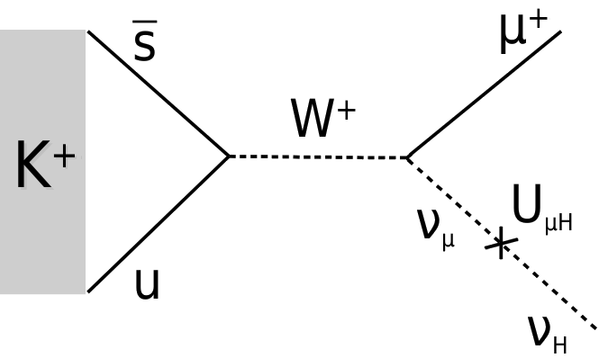
Figure 1: Production of a heavy sterile neutrino in the $\displaystyle K^{+}$ decay.

To contribute to the latter approach we analyzed a large data sample of $\displaystyle K^{+}\to\mu^{+}\nu$ recorded in 2012 by the OKA collaboration at IHEP-Protvino to search for a possible process $\displaystyle K^{+}\to\mu^{+}\nu_{H}$, see Fig. 1, where $\displaystyle\nu_{H}$ stands for one of the expected sterile $\displaystyle\nu_{H}$ according to the $\displaystyle\nu$MSM and $\displaystyle U_{\mu H}$ represents mixing element between SM muon neutrino and $\displaystyle\nu_{H}$.

2 Separated kaon beam and OKA experiment

The OKA experiment makes use of a secondary hadron beam of the U-70 Proton Synchrotron of NRC "Kurchatov Institute"-IHEP, Protvino, with enhanced fraction of kaons obtained by RF-separation with Panofsky scheme [13]. Corresponding deflectors are two superconducting Karlsruhe-CERN cavities used at SPS [14] and which were donated by CERN to IHEP in 1998. The cavities are cooled by superfluid He provided by the dedicated IHEP-build cryogenic system [15]. The design is optimized for the momentum of 12.5 and 17.7 GeV/c, the achieved fraction of kaons is up to 20% depending on the beam momentum, with the intensity of about $\displaystyle 5\times 10^{5}$ kaons per U-70 spill of 3 seconds duration. The r.m.s. width of the momentum distribution is estimated to be 1.5%.

The OKA setup, Fig. 2, is a magnetic spectrometer complemented by electromagnetic and hadron calorimeters and a Decay Volume. First magnet M₁ with surrounding 1 mm pitch PC’s (BPC_(1Y), BPC_(2Y,2X), BPC_(3X,3Y), BPC_(4X,4Y) of $\displaystyle\sim$1500 channels in total [16]) serves as a beam spectrometer.

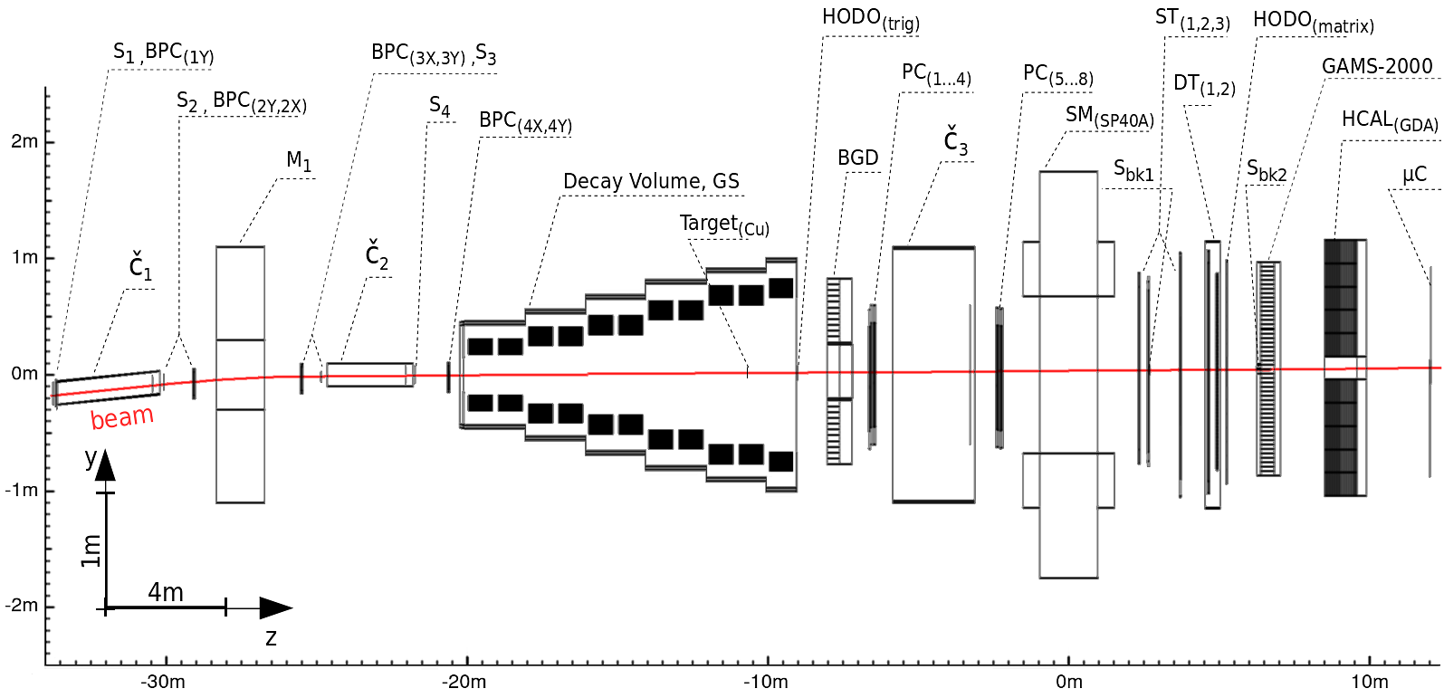
Figure 2: Schematic elevation view of the OKA setup, see text for details.

It is supplemented by two threshold Cherenkov counters Č₁, Č₂ for kaon selection and by beam trigger scintillation counters S₍₁₎, S₍₂₎, S₍₄₎, each of 200$\displaystyle\times$200$\displaystyle\times$1 mm³, and a thicker one, 60$\displaystyle\times$85$\displaystyle\times$6 mm³, delivering timing, S₍₃₎. The 11 m long Decay Volume (DV) filled with helium contains 11 rings of guard system (GS), which consists of 670 Lead-Scintillator sandwiches (20 layers of 1.5mm:5mm each) with WLS readout grouped in 300 ADC channels. To supplement GS, a gamma detector (BGD, made of $\displaystyle\sim$1050 5$\displaystyle\times$5$\displaystyle\times$42 cm³ lead glass blocks [17]), located behind the DV is used as a veto at large angles, while low angle particles pass through a central opening. The wide aperture 200$\displaystyle\times$140 cm² spectrometric magnet, SM_(SP40A), with a field integral of $\displaystyle\sim$1 Tm serves as a spectrometer for the charged decay products together with corresponding tracking chambers: 5k channels of 2 mm pitch PC’s (PC_1,…,8), 1k channels of 9 mm diameter straw tubes ST_(1,2,3) and 300 channels of 40 mm diameter drift tubes DT_1,2. The matrix hodoscope HODO_(matrix) is composed of 252 12$\displaystyle\times$12$\displaystyle\times$1.5 cm³ scintillator tiles with WLS+SiPM readout. It is used to improve time resolution and to link $\displaystyle x$–$\displaystyle y$ projections of a track. Two scintillator counters S_bk1, S_bk2 (80 mm and 90 mm in diameter with a thickness of 3.9 mm and 5 mm) serve to suppress undecayed beam particles. At the end of the OKA setup there are two calorimeters: electromagnetic (GAMS-2000 of $\displaystyle\sim$ 2300 3.8$\displaystyle\times$3.8$\displaystyle\times$45 cm³ lead glass blocks [18]) and a hadron one (HCAL_(GDA) of 100 20$\displaystyle\times$20$\displaystyle\times$108 cm³ iron-scintillator sandwiches with WLS plates readout [19]) and, finally, four partially overlapping muon counters $\displaystyle\mu$C (1$\displaystyle\times 1$ m² scintillators with WLS fibres readout) behind the HCAL.

3 Search for heavy neutrinos

A search for $\displaystyle K^{+}\to\mu^{+}\nu_{H}$ decay is done with the data set accumulated in November 2012 run with a 17.7 GeV/c beam momentum. Two prescaled triggers are used. The first one selects beam kaons which decay inside the OKA setup, $\displaystyle{\small\tt Tr_{Kdecay}=S_{1}\cdot S_{2}\cdot S_{3}\cdot S_{4}\cdot\check{C}_{1}\cdot\overline{\check{C}}_{2}\cdot\overline{S}_{bk}}$, prescale factor is 1/10, while the second one, $\displaystyle{\small\tt Tr_{K\to\mu X}=Tr_{Kdecay}\cdot{\mu}C}$, includes additionally muon counters $\displaystyle\mu$C and is prescaled by 1/4. The beam intensity (S${}_{1}\cdot$S${}_{2}\cdot$S${}_{3}\cdot$S₄) was $\displaystyle\sim 2\cdot 10^{6}$ per spill, the fraction of kaons in the beam is $\displaystyle\sim$ 12.5%, i.e. the kaon intensity is $\displaystyle\sim$250k/spill. The total number of $\displaystyle\sim 1.6\times 10^{10}$ events with kaon decays are logged.

3.1 Event selection

To select $\displaystyle K^{+}\to\mu^{+}$ $\displaystyle\nu$ decay channel in off-line analysis a set of requirements is applied:
– events with single beam track and single secondary track are selected;
– a single secondary track segment after the SM magnet is present in the event and it is well matched to showers of the muon type (i.e. one or two adjacent cells with the MIP energy deposition) in both GAMS-2000 and HCAL calorimeters;
– sufficient number of points on all the track segments is present to optimize the missing mass resolution;
– the momentum of kaon is consistent with that delivered by beam settings of $\displaystyle\approx 17.7$ GeV/c, while the required momentum of a secondary muon is below $\displaystyle 16.4$ GeV/c;
– to ensure good decay vertex reconstruction and also to suppress events in which kaon decays behind the DV, there is a requirement of 3 mrad minimal angle between the beam and the secondary track, and a requirement for the minimal distance between the beam and the secondary track to be $\displaystyle<1$ cm;
– the decay vertex is inside DV, and is further restricted to be 2$\displaystyle\sigma$ (of $\displaystyle z$-vertex resolution) from the DV entrance and the position of Cu-target;
– other decay channels are suppressed by requiring the total energy deposition in GS and BGD to be below 50 MeV/c² and 100 MeV/c², respectively;
– the total energy deposition in GAMS-2000 and HCAL should be consistent with that of a single muon.

After applying these cuts, $\displaystyle 26\times 10^{6}$ $\displaystyle K^{+}\to\mu^{+}\nu$ decays were selected for subsequent analysis.

3.2 Signal and background studies

A signal from heavy neutrino in $\displaystyle K^{+}\to\mu^{+}\nu_{H}$ may show up itself as a peak in the missing mass distribution, $\displaystyle m^{2}_{\nu}=m^{2}_{miss}=(p_{K}-p_{\mu})_{i}\cdot(p_{K}-p_{\mu})^{i}$, $\displaystyle i=1,2,3,4$. We assume that heavy sterile neutrinos are stable. The investigation of a possible signal decays and background contributions from kaon decays and from kaon scattering and interactions inside the OKA setup is done with detailed GEANT-3 simulation with the subsequent off-line reconstruction and analysis. Different decay channels simulated using Monte-Carlo are weighted according to corresponding matrix elements and branchings [20]. The experimental data and main backgrounds, which survived the selections cuts are shown in the $\displaystyle(m^{2}_{miss};p_{\mu})$ plots of Fig. 3.

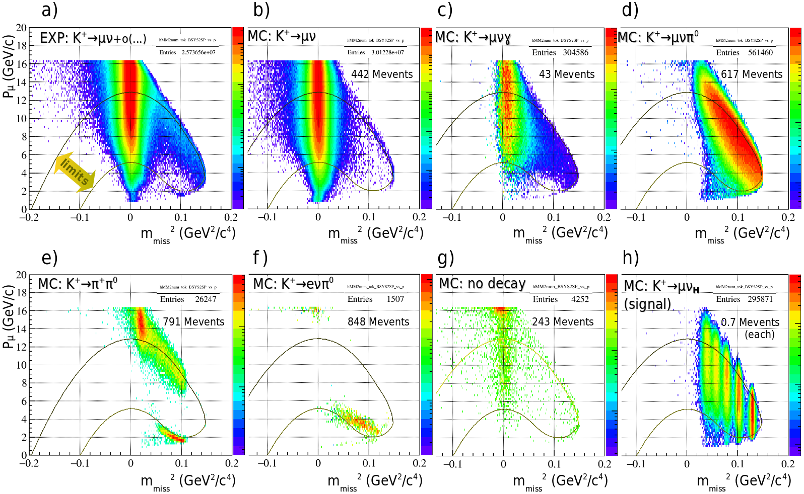
Figure 3: The distribution of $\displaystyle p_{\mu}$ vs. $\displaystyle m^{2}_{miss}$ obtained from the analysis of the experimental data (plot $\displaystyle a$) in comparison with Monte-Carlo simulation for the background channels (plots $\displaystyle b$, …, $\displaystyle g$) and for the set of signals (plot $\displaystyle h$) for $\displaystyle m_{\nu_{H}}=\{200,240,280,320,360\}$ MeV/c². Note logarithmic scale for the third dimension. Only events which passed the selection cuts are shown. In case of MC, the initial statistics is indicated.

In the region of low $\displaystyle m^{2}_{miss}$, both $\displaystyle K^{+}\to\mu^{+}\nu_{\mu}$ and $\displaystyle K^{+}\to\mu^{+}\nu_{\mu}\gamma$ dominate. In the region of $\displaystyle m^{2}_{miss}\gtrsim$ 0.05 GeV²/c⁴, the dominant contribution is given by $\displaystyle K^{+}\to\pi^{0}\mu^{+}\nu_{\mu}$ decay channel, which can not be excluded by kinematic cuts without significant loss in acceptance due to its rather flat distribution in the region of interest (see Fig. 3-d).

The $\displaystyle K^{+}\to\pi^{+}\pi^{0}$ decay channel is suppressed by four orders of magnitude, but it is responsible for a small peak at $\displaystyle m^{2}_{miss}$ around 0.1 GeV²/c⁴, which should be taken into account. Therefore we limit our acceptance (see Fig. 3-a) from the low muon momentum side by a smooth curve excluding the high event density spot from $\displaystyle K^{+}\to\pi^{+}\pi^{0}$ at low $\displaystyle p_{\mu}\approx 2$ GeV/c (see Fig. 3-e), while at high values of the muon momentum ($\displaystyle p_{\mu}$) we additionally introduce a smooth upper limit on $\displaystyle p_{\mu}$ to suppress a tail from badly reconstructed $\displaystyle K^{+}\to\mu^{+}\nu_{\mu}$ events. The contributions due to a misidentified electron from the $\displaystyle K^{+}\to e^{+}\nu_{e}\pi^{0}$ decay channel (Fig. 3-f) and from processes when kaon either scatters or interacts while passing the setup (Fig. 3-g) play a minor role.

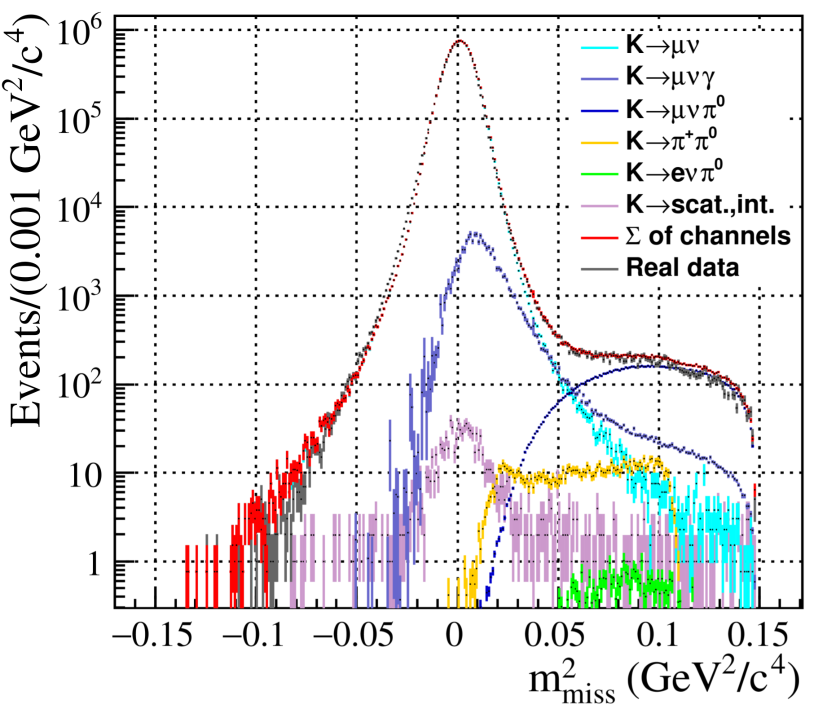
Figure 4: Missing mass distribution $\displaystyle m^{2}_{miss}$ for the data and MC events inside kinematic region, indicated in Fig. 3-a. Distribution for the experimental data is shown in gray, dominant decay channels, obtained from MC, are marked by different colors, while their sum is depicted in red. The normalization is relative to the experimental data.
 

Missing mass distribution $\displaystyle m^{2}_{miss}$ for the data and MC events inside kinematic region, indicated in Fig. 3-a, is shown in Fig. 4. The distribution for the experimental data is shown in gray, dominant decay channels, obtained from simulation, are marked by different colors with the explanation in the top-right corner, while their sum is depicted in red. The normalization is done to the experimental data at $\displaystyle m^{2}_{miss}=0$. The relative normalization of different channels is done in accordance with their branching ratios. As seen from Fig. 4, there is a reasonable agreement between the experimental and MC data with some discrepancy in the $\displaystyle m^{2}_{miss}>0.05$ GeV²/c⁴ region. Since contributions from different background sources are strongly suppressed (by orders of magnitude) by our selection criteria, one may expect that efficiencies obtained from MC simulations are reproduced not at the same level of accuracy as it is the case for the main decay channel, $\displaystyle K^{+}\to\mu\nu_{\mu}$. To account for that we do a fit, introducing an additional multiplication constant for each of the suppressed background sources. The fit is done within a region of $\displaystyle m^{2}_{miss}>0.05$ GeV²/c⁴, see Fig. 6.

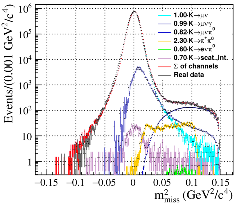
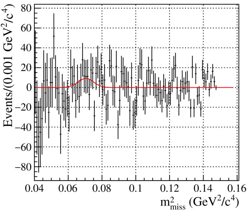
Figure 5: Same as Fig. 4, but magnitudes of individual MC-simulation terms are tuned by the fit procedure for the best agreement with the data in the region of $\displaystyle m^{2}_{miss}>0.05$ GeV²/c⁴. Multiplicative efficiency correction is indicated for each background term.

Figure 6: The residual signal distribution after subtraction of the fitted background (see Fig. 6) from the experimental data in the range of $\displaystyle m^{2}_{miss}>0.05$ GeV²/c⁴. An example of the fit for the signal with the certain $\displaystyle m_{\nu_{H}}$ and appropriate width is shown by the red curve.  

3.3 Signal search with a subtraction of the MC-simulated background

As a next step, the obtained background curve is subtracted (see Fig. 6) for the subsequent search for heavy neutrinos. For the signal search, a parametrization of the signal shape is essential. For that, a set of reconstructed heavy neutrino signals was produced by the MC simulation with a neutrino mass step of 20 MeV/c². The signal, as a function of $\displaystyle m^{2}_{miss}$, can be approximated by the Gaussian shape, with an integral error of $\displaystyle\sim$2%. Interpolation for the signal width between the generated set of masses is done with polynomial curves. The same method is used to produce a total efficiency curve $\displaystyle\varepsilon_{\nu_{H}}$, see Fig. 7.

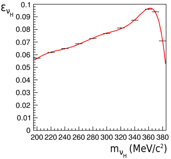
Figure 7: The $\displaystyle m_{\nu_{H}}$ dependence of the total efficiency of the signal obtained for the set of values of heavy neutrino mass. The interpolation curve is also shown.  

After that, we do series of fits of the residual distribution of Fig. 6 with a Gaussian shape signal at given mass with an appropriate width i.e. the only parameter of the fit is the signal integral which is not restricted by positive values. The obtained number of events $\displaystyle N_{\nu_{H}}$ is shown with corresponding errors for each fit in Fig. 9.

No indications of signal from $\displaystyle\nu_{H}$ is found in the mass region of interest. The signal significance does not exceed two standard deviations in the studied mass interval. Since the number of events in each bin in the considered $\displaystyle m^{2}_{miss}$-region is sufficiently high $\displaystyle\sim 10^{2}$ one can apply here the Wald approximation for the likelihood ratio method of upper limits calculation for single parameter of interest [21, 22] which leads to the following single-sided upper limit for the signal at 90% CL:

$\displaystyle N^{(Upp.Lim.)}_{\nu_{H}}=1.28\cdot\sigma+N^{(fit)}_{\nu_{H}}$,     for $\displaystyle N^{(fit)}_{\nu_{H}}\geq 0$,

$\displaystyle N^{(Upp.Lim.)}_{\nu_{H}}=1.28\cdot\sigma$,                for $\displaystyle N^{(fit)}_{\nu_{H}}<0$,

where $\displaystyle\sigma$ is the standard deviation estimated from the fit, while multiplier of 1.28 corresponds to one-sided estimate with 90% CL for the Gaussian case. The results are shown in Fig. 9.

From that, an upper limit on branching, see bold curve $\displaystyle(a)$ at Fig. 9, is obtained by normalization to the decay $\displaystyle K^{+}\to\mu\nu_{\mu}$:

$$Br(K^{+}\to\mu\nu_{H})=Br(K^{+}\to\mu\nu_{\mu})\cdot\frac{N_{\nu_{H}}}{\varepsilon_{\nu_{H}}}\cdot\frac{\varepsilon_{\nu_{\mu}}}{N_{\nu_{\mu}}},$$

where $\displaystyle\varepsilon_{\nu_{H}}$ is obtained from the interpolation function of $\displaystyle m_{miss}$, see Fig. 7, $\displaystyle N_{\nu_{\mu}}=12.6\times 10^{6}$ is a number of reconstructed $\displaystyle K^{+}\to\mu\nu_{\mu}$ events from the experimental data and its efficiency $\displaystyle\varepsilon_{\nu_{\mu}}=0.039$ is known from the simulation; efficiencies and absolute values mentioned here refer to the limited kinematic area (defined in Fig. 3-a).

It should be noted that the exclusion of background contributions from $\displaystyle K^{+}\to e^{+}\nu_{\mu}\pi^{0}$ (Fig. 3-f) and from undecayed kaon (Fig. 3-g) does not change the obtained results.

Figure 8: Number of signal-like heavy neutrino events $\displaystyle N_{\nu_{H}}$ obtained from the fit of the residual distribution for different values of $\displaystyle m^{2}_{\nu_{H}}$ (black points), vertical error bar stands for one standard deviation, $\displaystyle\sigma$. Solid curve corresponds to the upper limit for the number of signal events at 90% CL.

Figure 9: Upper limit for $\displaystyle Br(K^{+}\to\mu\nu_{H})$ at 90% CL as a function of a heavy neutrino mass for three procedures of fit: the bold curve $\displaystyle(a)$ represents procedure described in subsection 3.3, while curves $\displaystyle(b)$ and $\displaystyle(c)$ are obtained in subsection 3.4 within simultaneous signal and background fit procedures.

3.4 Upper limits with a common fit of signal and background

As an alternative we do a series of fits of the initial $\displaystyle m^{2}_{miss}$ distribution of Fig. 6 for $\displaystyle m^{2}_{miss}>0.05$ GeV${}^{2}/c^{4}$ with a sum of Gaussian signal for a given mass and all the MC background sources, again, with additional multiplication coefficients which now may vary from point to point. Such a procedure is more favorable for the signal amplitude as compared to that of subsection 3.3, where the background is estimated once before the subtraction and, hence, gives more conservative estimate for the upper limit. The remaining part for the calculation of upper limits is done in the same way and the result is indicated in Fig. 9 by a thin smooth curve $\displaystyle(b)$.

To confirm the obtained results we end up with a simplified approach, less dependent on MC, where the background contribution is taken from a 5-th order polynomial approximation of the $\displaystyle m^{2}_{miss}$ distribution of the experimental data within the range of $\displaystyle m^{2}_{miss}>0.05$ GeV${}^{2}/c^{4}$. Again we do a common fit for signal plus background, where we allow the tuning of the background parameters for each investigated position. In this case the obtained upper limit at 90% CL is shown with dashed curve $\displaystyle(c)$ in Fig. 9.

Finally we select the result obtained with the MC background model described in subsection 3.3 as the main one, while the difference between three curves in Fig. 9 can be treated as a systematic error of the method.

3.5 Evaluation of the $\displaystyle|U_{\mu H}|^{2}$ mixing parameter upper limit

Finally, we obtain an upper limit on the mixing parameter $\displaystyle|U_{\mu H}|^{2}$ between the muon neutrino and the heavy sterile neutrino $\displaystyle\nu_{H}$, see Fig. 10. The coupling strength (see Fig. 1) between muon neutrino and $\displaystyle\nu_{H}$ is obtained from the relation:

$$\frac{\Gamma(K\to\mu\nu_{H})}{\Gamma(K\to\mu\nu_{\mu})}=|U_{\mu H}|^{2}\cdot\lambda\cdot f_{\mathfrak{M}},$$

where $\displaystyle\lambda$ is a kinematic factor, $\displaystyle f_{\mathfrak{M}}$ is a helicity factor in the matrix element, both arising for the case of massive neutrino in the final state [23].

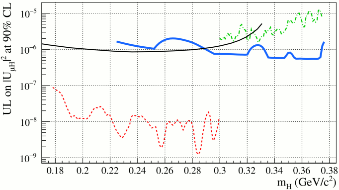
Figure 10: The OKA upper limit on the mixing matrix element $\displaystyle|U_{\mu H}|^{2}$ at 90% CL is shown with solid blue curve, in comparison with preceding experiments: the black curve represents the result from KEK-E-089 [10], the red dashed curve corresponds to the result from BNL-E949 [11] obtained with stopped kaons, while the dash-dotted green curve indicates the recent result from CERN-NA62 [12]

Since the obtained upper limit on $\displaystyle|U_{\mu H}|^{2}$ in the considered mass range does not exceed $\displaystyle 10^{-5}$, the $\displaystyle\nu_{H}$ mean life time is estimated to be greater than $\displaystyle 10^{-6}$ sec, assuming it decays to SM particles, [12]. The corresponding $\displaystyle\nu_{H}$ mean flight distance, estimated with a MC simulation for the $\displaystyle\nu_{H}$ masses considered, ranges between 5–25 km. Hence the heavy neutrino in our case, indeed, can be regarded as stable particle.

Conclusions

The OKA 2012 data set was analyzed to search for heavy sterile neutrinos. A peak search method in the missing mass spectrum was used in the analysis. No signal is seen and the upper limit on the mixing between muon neutrino and a heavy sterile neutrino is set in the mass range 300–375 MeV/c².

Our result improves the old limit from KEK [10] and the recent result from CERN NA62 [12] for the mass range $\displaystyle m_{H}>290$ MeV/c², while at lower masses we still do not reach sensitivity of BNL-E949 [11].

References

- [1] Y. Fukuda et al., Evidence for oscillation of atmospheric neutrinos, Phys. Rev. Lett. 81, 1562 (1998); arXiv:hep-ex/9807003.
- [2] Q. R. Ahmad et al., Direct Evidence for Neutrino Flavor Transformation from Neutral-Current Interactions in the Sudbury Neutrino Observatory, Phys. Rev. Lett. 89, 011301 (2002); arXiv:nucl-ex/0204008.
- [3] K. Eguchi et al., A High Sensitivity Search for ’s from the Sun and Other Sources at KamLAND, Phys. Rev. Lett. 92, 071301 (2004); arXiv:hep-ex/0310047.
- [4] M. H. Ahn et al., Measurement of Neutrino Oscillation by the K2K Experiment, Phys. Rev. D74 (2006) 072003; arXiv:hep-ex/0606032.
- [5] T. Asaka et al., The MSM, Dark Matter and Neutrino Masses, Phys. Lett. B631:151-156, 2005; arXiv:hep-ph/0503065.
- [6] L. Canetti et al., Dark Matter, Baryogenesis and Neutrino Oscillations from Right Handed Neutrinos; Phys. Rev. D 87, 093006 (2013); arXiv:1208.4607 (2012).
- [7] D. Gorbunov et al., How to find neutral leptons of the MSM?, JHEP 0710 (2007) 015 (2007), Erratum: JHEP 1311 (2013) 101.
- [8] G. Bernardi, et al., Search for Neutrino Decay, Phys.Lett. 166B (1986) 479-483.
- [9] V. Duk et al, Search for Heavy Neutrino in Decay at ISTRA+ Setup, Phys. Lett. B710 (2012) 307-317.
- [10] R. S. Hayano et al., Heavy-Neutrino Search Using K2 Decay, Phys. Rev. Lett. 49, 1305 (1982).
- [11] A. Artamonov et al., Search for heavy neutrinos in decays, Phys. Rev. D91 (2015) no.5, 052001.
-
[12]
C. Lazzeroni et al., Search for Heavy Neutrinos in Decays, Phys. Lett. B772 (2017) 712-718; arXive:1705.07510 (2017).
F. Newson, Kaon identification and the search for heavy neutrinos at NA62, Ph.D. thesis (2016), University of Birmingham. - [13] V. I. Garkusha et al., IHEP preprint, IHEP 2003-4.
- [14] A. Citron et al., The Karlsruhe-CERN Superconducting RF Separator, Nucl. Instrum. Meth. 164 (1979) 31-35.
- [15] A. Ageev et al., Proceedings of RUPAC-2008, p.282.
-
[16]
A. Yu. Petrus, B. Zh. Zalikhanov, Electro-mechanical properties of narrow-gap multiwire proportional chambers, Nucl. Instrum. Meth. A485 (2002) 399-410; JINR-E13-2001-113.
E. M. Gushchin et al., Fast beam chambers of the setup ISTRA-M, Nucl. Instrum. Meth. A351 (1994) 345-348. - [17] B. Powell et al., The EHS Lead Glass Calorimeters and Their Laser Based Monitoring System, Nucl. Instrum. Meth. 198 (1982) 217.
- [18] F. G. Binon et al., Hodoscope Multi-Photon Spectrometer Gams-2000, Nucl. Instrum. Meth. A248 (1986) 86; IFVE-85-62.
- [19] F. G. Binon et al., Modular Hadron Calorimeter (In Russian), Preprint IHEP, Protvino 1986, 86-109, IFVE-86-109.
- [20] C. Patrignani et al., (Particle Data Group), Chin. Phys. C, 40, 100001 (2016).
- [21] G. Cowan et al. Asymptotic formulae for likelihood-based tests of new physics, Eur. Phys. J. C71, 1554 (2011); arXiv:1007.1727.
- [22] A. Wald, Tests of Statistical Hypotheses Concerning Several Parameters When the Number of Observations is Large, Transactions of the American Mathematical Society, Vol. 54, No. 3 (1943) pp. 426-482.
- [23] R. E. Shrock, General theory of weak processes involving neutrinos. I. Leptonic pseudoscalar-meson decays, with associated tests for, and bounds on, neutrino masses and lepton mixing, Phys. Rev. D24, 1232 (1981).