Subspace Segmentation by Successive Approximations: A Method for Low-Rank and High-Rank Data with Missing Entries

Abstract

We propose a method to reconstruct and cluster incomplete high-dimensional data lying in a union of low-dimensional subspaces. Exploring the sparse representation model, we jointly estimate the missing data while imposing the intrinsic subspace structure. Since we have a non-convex problem, we propose an iterative method to reconstruct the data and provide a sparse similarity affinity matrix. This method is robust to initialization and achieves greater reconstruction accuracy than current methods, which dramatically improves clustering performance. Extensive experiments with synthetic and real data show that our approach leads to significant improvements in the reconstruction and segmentation, outperforming current state of the art for both low and high-rank data.

1 Introduction

Linear Subspaces are one of the most powerful mathematical objects to represent and model high-dimensional data. Machine Learning and especially Computer Vision communities use these tools in a wide variety of algorithms in domains such as classification, structure-from-motion, object recognition and image-segmentation. However, in all the above areas, observations in real scenarios are incomplete due to self-occlusion, sensor failure or data corruption, to name a few.

In this paper specifically, we address the problem of subspace clustering with missing data by simultaneously completing the data and enforcing a subspace structure. So, given a set of incomplete high-dimensional points drawn from a union of linear subspaces, we aim to estimate the unknown data and segment the reconstructed data points. For example, in Figure LABEL:fig:cars_frames, we focus on the long standing problem of motion segmentation in a scenario with strong occlusion and unreliable feature tracking. The task is to compute the complete feature point trajectories and cluster them according to the motion of the multiple rigid objects in the scene (e.g., cars, background).

The problem stated above boils down to answering two fundamental questions: 1) how to reconstruct the data from the observed entries and; 2) how to aggregate data such that each cluster lies on a linear subspace. Some recent developments attempt to tackle both problems jointly, however, the bulk of published work approaches each of the subproblems separately. For simplicity, we categorize prior work in two main classes: 1) methods that do subspace clustering considering only observed data (e.g., [31]) and; 2) methods that reconstruct the data assuming it lies on one single subspace and then proceed with the segmentation (e.g., [27]).

We propose a method called Subspace Segmentation by Successive Approximations (SSSA), that unifies the reconstruction of the data and the subspace structure of the clusters. Using a sparse representation of the data [7, 5], we achieved greater accuracy on the estimates of the missing data, that greatly improved the segmentation. Extensive experiments prove that this strategy significantly outperforms current state of the art, being able to achieve zero clustering error with up to $70\%$ of data missing in low and high-rank data.

2 Related Work

Most of the state of the art methods for subspace recovery approach the problem without considering the recovery of the missing data, leading to biased and skewed estimates of the subspaces. Thresholding-based Subspace Clustering (TSC), builds an affinity matrix based on the inner product between incomplete (zero-filled) data points [15], severely impacting the affinity as the fraction of missing data increases. Recently, [31] proposes the Sparse Subspace Clustering by Entry-Wise-Zero-Fill (SSC-EWZF), generalizing Sparse Subspace Clustering (SSC) [10] by filling the data matrix with zeros in the missing entries and evaluating the error only in the known entries. Also in [31], the authors propose the SSC by Column-wise Expectation-based Completion (SSC-CEC), which solves the SSC with an estimated kernel matrix in place of the incomplete data matrix. Within this group, several methods assume the rank of the subspaces is known a priori. In [1], the authors initialize $k$ subspaces of known dimensions with the probabilistic farthest insertion and iteratively update the subspaces by minimizing the data projection residuals. Based on subset selection, [12] estimates and refines the subspaces of maximum known rank. Missing entries are then estimated by projecting the data onto the assigned subspace. Group-sparse subspace clustering (GSSC), proposed in [20], estimates the subspace bases that best fit the known entries in the data.

An alternative approach is to first estimate the missing data with low-rank matrix completion methods [6], [4], [30] and then segment the data with SSC [10] or low-rank subspace clustering [26]. Also, in the context of motion segmentation, [27] applies the PowerFactorization method to estimate missing entries after projecting the points onto a low-dimensional space. GPCA is then used to fit linear subspaces to the data [28].

Finally, the other approaches jointly recover the missing data and the subspaces. In [13], the problem is formulated as one of factor analysis, using a mixture of probabilistic PCA to model the data. Mixture models are also proposed in [19] and [20]. The first considers the usual framework of mixture of Gaussians, extending the mixture probabilistic principal component analysers [25] to missing data. The second proposes the Mixture Subspace Clustering (MSC), which finds the mixture of data projections (onto each subspace) that best fits the known entries of the data, while minimizing the rank of these projections. [29] proposes a solution specially tailored for recovering and clustering incomplete images, using total variation regularization for the image restoration. More recently, [9] proposed an extension to SSC where the missing data and coefficients are jointly estimated. Noting that the outer product of a subset of missing entries and coefficients is a rank $1$ matrix, the author proposes the nuclear norm as regularizer. However, it is known that using the nuclear norm to impose a desired rank $r$ may severely distort the $r$ highest singular values, resulting in poor solutions [3], [16].

In summary, state of the art methods either use only the observed data, providing biased estimates of the subspaces [15], [31], [1], [12], [20], or impose global constraints that assume the data lies on one single subspace, failing to impose the subspace model when reconstructing the data [6], [4], [30], [27], or impose inadequate models, failing to jointly recover data and subspaces [13], [19], [20], [9].

3 Subspace Segmentation by Successive Approximations

In this section, we propose a method to estimate the missing entries of a partially prescribed matrix and to segment the reconstructed data into clusters corresponding to the underlying subspaces. We build upon the work Sparse Subspace Clustering [10] and explicitly represent the missing data.

Consider $K$ subspaces $\{\mathcal{S}_{k}\subset\mathbb{R}^{D}\}_{k=1}^{K}$, with dimensions $\{d_{k}<D\}_{k=1}^{K}$, and let $\{\mathbf{x}_{j}\in\mathbb{R}^{D}\}_{j=1}^{N}$ be the set of $N$ data points lying in the union of the $K$ subspaces (see footnote for notation). Denote the data matrix as $\mathbf{X}=[\mathbf{x}_{1}\,\mathbf{x}_{2}\dots\mathbf{x}_{N}]\in\mathbb{R}^{D\times N}$, where each $\mathbf{x}_{j}$ is a data point. Since only a subset of the entries is observed, we can define $\mathbf{X}$ as

$$\mathbf{X}=\mathbf{X}_{\Omega}+\mathbf{X}_{\Omega^{\complement}},$$ (1)

where $\mathbf{X}_{\Omega}$ is a matrix with the known entries at $(i,j)\in\Omega$, and zero otherwise. $\mathbf{X}_{\Omega^{\complement}}$ is the matrix with the missing entries in the complementary positions, $(i,j)\in\Omega^{\complement}$, and zero otherwise. To recover the original subspaces, we first estimate the unknown $\mathbf{X}_{\Omega^{\complement}}$ by imposing the subspace model and then cluster the recovered data points. The missing data is estimated by solving the following optimization problem

$$\min_{\mathbf{X}_{\Omega^{\complement}},\mathbf{C},\mathbf{E},\mathbf{Z}}\quad \left\lVert\mathbf{C}\right\rVert_{1}+\lambda_{e}\left\lVert\mathbf{E}_{\Omega}\right\rVert_{1}+\frac{\lambda_{z}}{2}\left\lVert\mathbf{Z}_{\Omega}\right\rVert_{F}^{2}$$ (2)

s.t. $$\mathbf{X}_{\Omega}+\mathbf{X}_{\Omega^{\complement}}=\left(\mathbf{X}_{\Omega}+\mathbf{X}_{\Omega^{\complement}}\right)\mathbf{C}+\mathbf{E}+\mathbf{Z}$$

$$diag(\mathbf{C})=0.$$

The first constraint of (2), translates the self-expressiveness property, which exploits the fact that each data point in a union of subspaces can be represented as a linear or affine combination of other points. By minimizing the $\ell_{1}\text{-norm}$ of the coefficients matrix, $\mathbf{C}$, we favor a sparse representation of the data, in which, ideally, a point is represented by a linear combination of few points from its own subspace [7, 5]. The second and third terms in the cost function account for the sparse error, $\mathbf{E}$, and noise, $\mathbf{Z}$, in the known entries, respectively. For complete data, this model is guaranteed to recover the desired representation when the subspaces are sufficiently separated and data points are well distributed inside the subspaces [11, 22, 23].

We depart from [31] by imposing the model to both complete and incomplete data and dealing with outliers, we dramatically improve the recovery of the underlying subspaces, providing a better fit to the known entries of the data. The problem becomes non-convex because of the product between $\mathbf{X}_{\Omega^{\complement}}$ and $\mathbf{C}$, so, in the next section, we propose an iterative algorithm to solve (2). Finally, after solving the optimization problem, we build an affinity matrix from $\mathbf{C}$ and apply spectral clustering to segment the data in $K$ clusters.

3.1 Solving the Optimization Problem

First, we note that (2) is convex when one of the variables, $\mathbf{X}_{\Omega^{\complement}}$ or $\mathbf{C}$, is fixed. So, similar to [14], we propose a two step iterative algorithm, in a Expectation-Maximization (EM) approach [8]. On the E-step we estimate the missing data given the current model (subspaces). On the M-step we estimate the subspaces given the current missing data. This procedure is outlined in Algorithm 1.

Algorithm 1 Subspace Segmentation by Successive Approximations

1:Input: $\mathbf{X}$ - Incomplete data matrix

2:   $\Omega$ - Set of indexes of known entries

3:   $\lambda_{e}$, $\lambda_{z}$ - Error trade off parameters

4:   $K$ - Number of subspaces

5:Output: $\hat{\mathbf{X}}$ - Estimated data matrix

6:    ​$\mathbf{C}$ - Coefficients

7:    ​​$labels$ - Point labels

8:

9:

10:

11:$\mathbf{X}_{\Omega^{\complement}}^{(0)}\leftarrow$ Initialize

12:$\mathbf{C}^{(0)}\leftarrow$ Fixing $\mathbf{X}_{\Omega^{\complement}}$ as $\mathbf{X}_{\Omega^{\complement}}^{(0)}$, solve (2)

13:while not convergence do

14:      E-Step

15:     $\mathbf{X}_{\Omega^{\complement}}^{(i+1)}\leftarrow$ $(\mathbf{X}^{(i)}\mathbf{C}^{(i)})_{\Omega^{\complement}}$

16:      M-Step

17:     $\mathbf{C}^{(i+1)}\leftarrow$ Fixing $\mathbf{X}_{\Omega^{\complement}}$ as $\mathbf{X}_{\Omega^{\complement}}^{(i+1)}$,

18:                  solve (2)

19:$labels\leftarrow$ SpectralClustering($K$,$\mathbf{C}$)

The initialization step in line 11 provides an initial guess for the missing entries, like zeros in all entries, the (feature-wise) mean of the known entries or random initialization. In line 15, we update the unknown entries with its current estimates, $\mathbf{X}_{\Omega^{\complement}}^{(i+1)}=(\mathbf{X}^{(i)}\mathbf{C}^{(i)})_{\Omega^{\complement}}$. In the M-step, line 17, we solve (2) but with fixed $\mathbf{X}_{\Omega^{\complement}}=\mathbf{X}^{(i+1)}_{\Omega^{\complement}}$. Finally, in line 19, we use the spectral clustering algorithm.

4 Experiments

In this section, we assess the performance of our method and compare it to state of the art methods. We consider two metrics: clustering error and reconstruction error, defined as

$$e_{c}=\frac{\#\text{missclassified points}}{\#\text{points}}, e_{r}=\frac{||\hat{\mathbf{X}}-\mathbf{X}||_{F}}{\left\lVert\mathbf{X}\right\rVert_{F}},$$ (3)

where $\hat{\mathbf{X}}$ and $\mathbf{X}$ are the estimated and true data matrices, respectively, and $\left\lVert.\right\rVert_{F}$ the Frobenius norm.

We compare our algorithm with SSC-EWZF [31], MSC [20], SSC-Lifting [9], TSC [15], the EM algorithm for subspace clustering (EMSC) [19] and matrix completion [4] followed by SSC (MC-SSC). The parameters of each algorithm were set according to the authors suggestions and in order to minimize the clustering error in a test set.

In our experiments, we initialized the missing entries with the mean or zeros and use spectral clustering [18] with affinity matrix $|\mathbf{C}|+|\mathbf{C}|^{T}$. We solve (2) with Algorithm 1. The M-step of the algorithm can be solved with the alternating direction method of multipliers (ADMM) [2].

4.1 Synthetic Data

We draw $N_{k}$ points per subspace from a union of $K$ random subspaces of dimension $d\ll D$ in $\mathbb{R}^{D}$. For simplicity, we draw the same number of points $N_{k}$ per subspace $k\in\{1,\dots,K\}$ and assume all subspaces have dimension $d\leq N_{k}$. The missing data is generated by selecting uniformly at random, with probability $\rho$, the set of entries corresponding to missing values, $\Omega^{\complement}$.

To benchmark the performance of the methods, we evaluate the impact of the rank of the data matrix by running the methods with low-rank and high-rank data. In the low-rank (LR) case we have: $K=3$, $D=50$, $d_{k}=5$, $N_{k}=20$. Unless stated otherwise, in the high-rank (HR) case we have $K=10$, $D=80$, $d_{k}=10$, $N_{k}=50$. Moreover, we study the impact of the missing rate, ambient space dimension and number of points per subspace in the reconstruction and clustering errors. Finally, we assess the performance of our method when the data is corrupted with noise or outlying entries.

4.1.1 Reconstruction Error

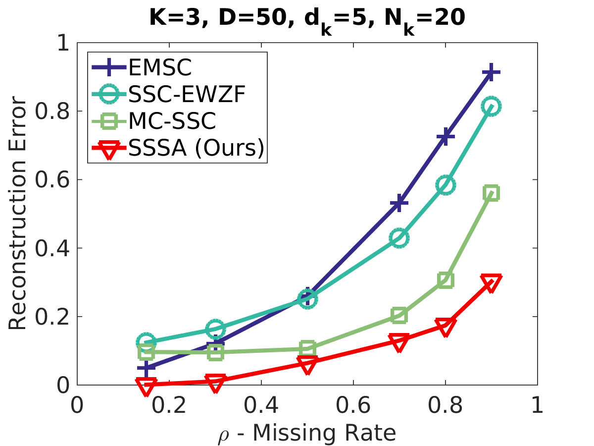
(a) Varying $\rho$ in low-rank.

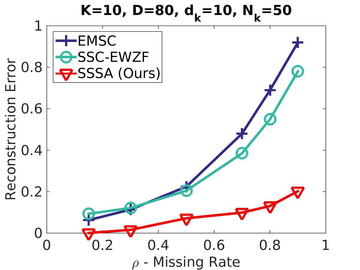
(b) Varying $\rho$ in high-rank.

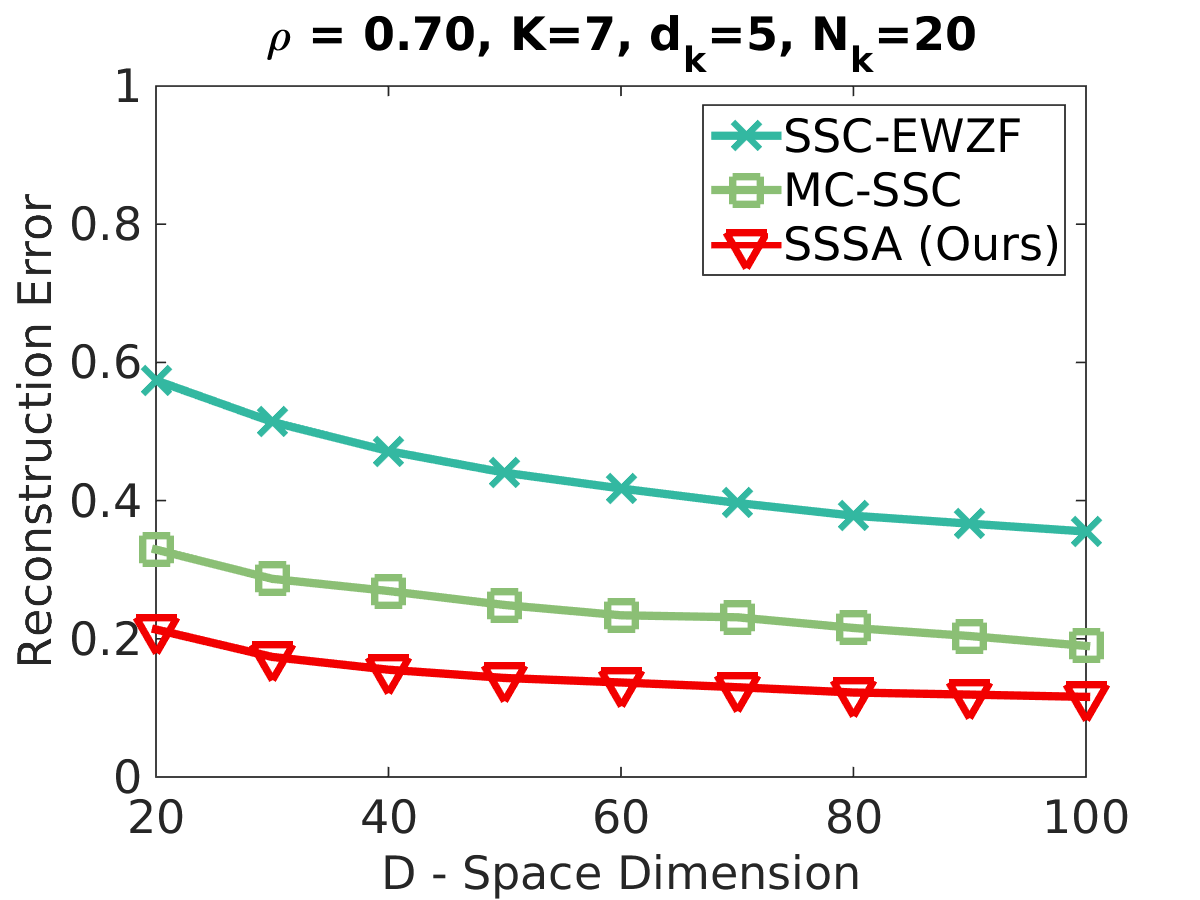
(c) Varying $D$.

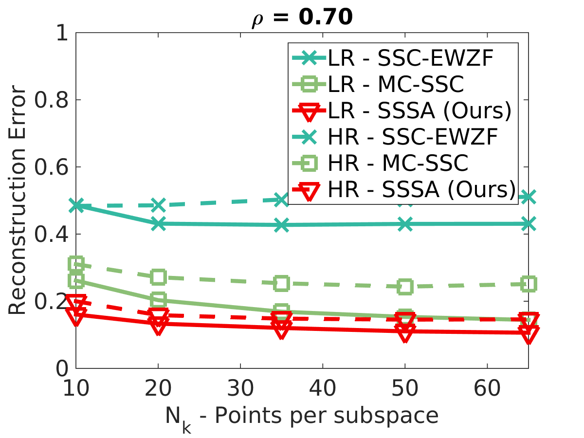
(d) Varying $N_{k}$.

Figure 1: Reconstruction error: (a) as a function of missing rate, $\rho$, for LR case; (b) as a function of missing rate, $\rho$, HR case; (c) as a function of the ambient space dimension, $D$, with $\rho=0.70$, $N_{k}=20$, $K=7$ and $d=5$; (d) as a function of the number of points per subspace, $N_{k}$, with $\rho=0.70$ for low-rank ($K=3$, $d=5$, $D=50$) and high-rank ($K=7$, $d=5$, $D=35$).

Figures 1a-1b show the reconstruction error as a function of the missing probability, $\rho$, for LR and HR cases, respectively. In both cases, SSSA outperforms other methods. This is specially noticeable for higher missing rates, where only MC-SSC comes close in low-rank. However, this method is intrinsically inadequate for high-rank data.

Figure 1c shows the error versus the ambient space dimension $D$, going from high to low-rank. In this experiment we have $\rho=0.70$, $N_{k}=20$, $K=7$ and $d=5$. As before, SSSA has significantly lower error, which is crucial in achieving a good subspace segmentation, as we will see in the next section. With a more favorable case ($\rho=0.30$ and $N_{k}=100$), SSC-Lifting has higher reconstruction errors, as reported by the author in [9]. With $D=20$, it reports $e_{r}\approx 0.495$ and with $D=30$, $e_{r}\approx 0.36$. Moreover, this method is computationally expensive, as for each missing entry it introduces $N$ new variables, with $N=\sum_{k}^{K}N_{k}$, exponentially increasing the size of the problem as $\rho$ or $N_{k}$ increase.

Figure 1d shows the reconstruction error as a function of the number of points per subspace for low-rank ($K=3$, $d=5$, $D=50$) and high-rank ($K=7$, $d=5$, $D=35$) cases, with $\rho=0.70$. Although all methods have approximately constant error as $N_{k}$ increases, SSSA has lower error in both low and high-rank, with very similar results in both cases.

4.1.2 Clustering Error

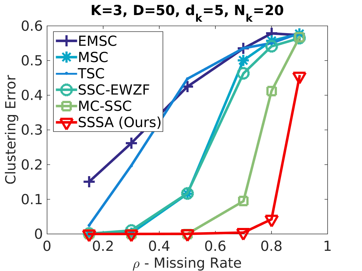
(a) Varying $\rho$ in low-rank.

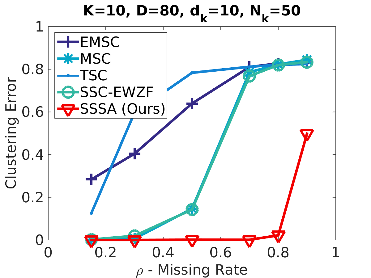
(b) Varying $\rho$ in high-rank.

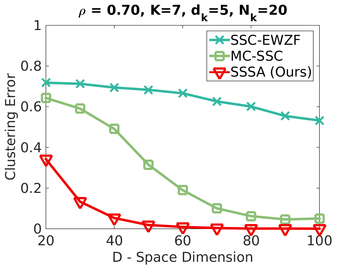
(c) Varying $D$.

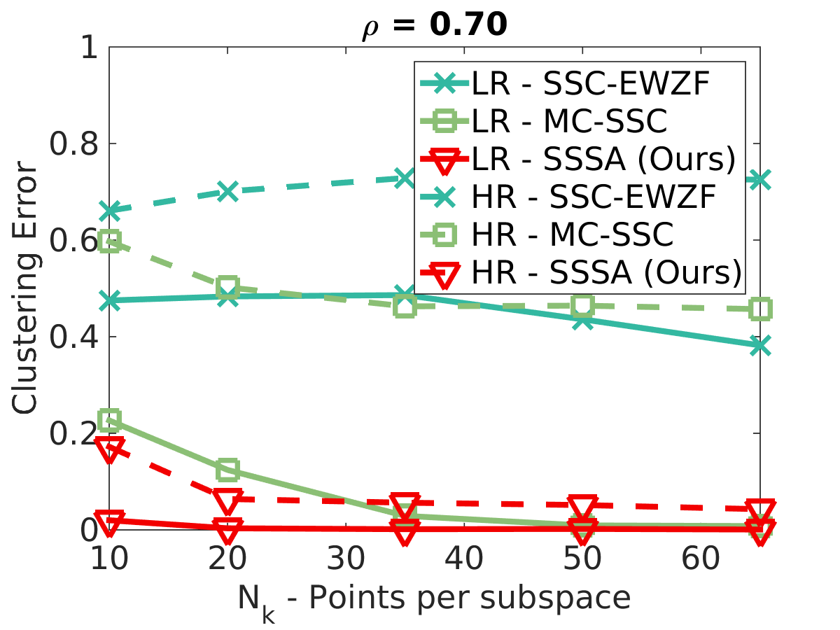
(d) Varying $N_{k}$.

Figure 2: Reconstruction error: (a) as a function of missing rate, $\rho$, for LR case; (b) as a function of missing rate, $\rho$, HR case; (c) as a function of the ambient space dimension, $D$, with $\rho=0.70$, $N_{k}=20$, $K=7$ and $d=5$; (d) as a function of the number of points per subspace, $N_{k}$, with $\rho=0.70$ for low-rank ($K=3$, $d=5$, $D=50$) and high-rank ($K=7$, $d=5$, $D=35$).

Figures 2a and 2b show the clustering error as a function of $\rho$ for LR and HR. SSSA has significantly lower errors in the harder cases, with high missing rates. We should note that SSC-EWZF is equivalent to SSSA first iteration if we initialize the missing entries with zeros and there are no outliers in the data. However, the difference in performance between SSSA and SSC-EWZF highlights the improvement achieved by the iterative approach we propose for the subspace recovery.

Figure 2c shows the clustering error as a function of $D$ for $\rho=0.70$, $N_{k}=20$, $K=7$ and $d=5$. The gap between SSSA and other methods reinforces, once again, the dramatic improvement that our method brings over the state of the art methods in the harder cases, i.e., high-rank data and high missing rates.

Finally, Figure 2d shows the clustering error versus $N_{k}$ for the same cases as Figure 1d. With $70\%$ missing data, in any scenario, our method has meaningful gains in the clustering performance. MC-SSC error decreases as $N_{k}$ increases but it still has large errors in the high-rank case.

4.1.3 Noise and Outliers

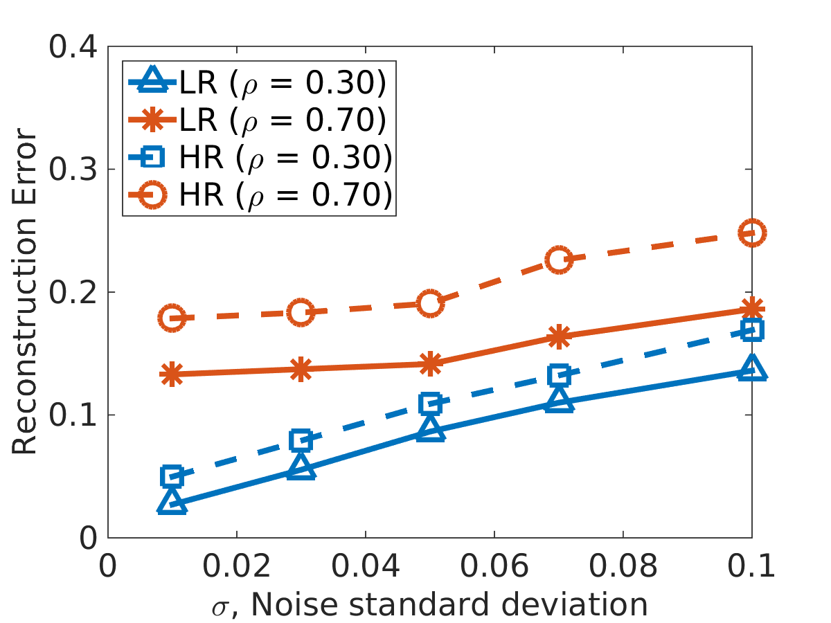
(a)

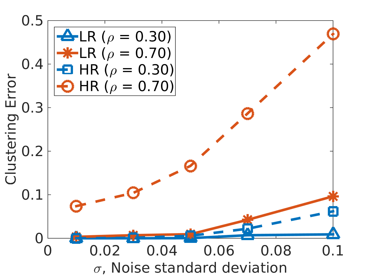
(b)

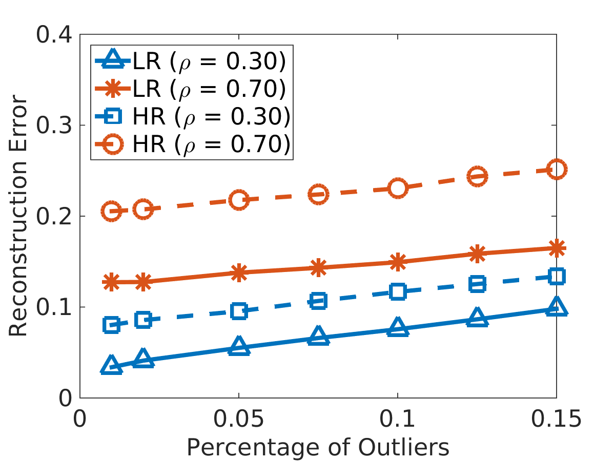
(c)

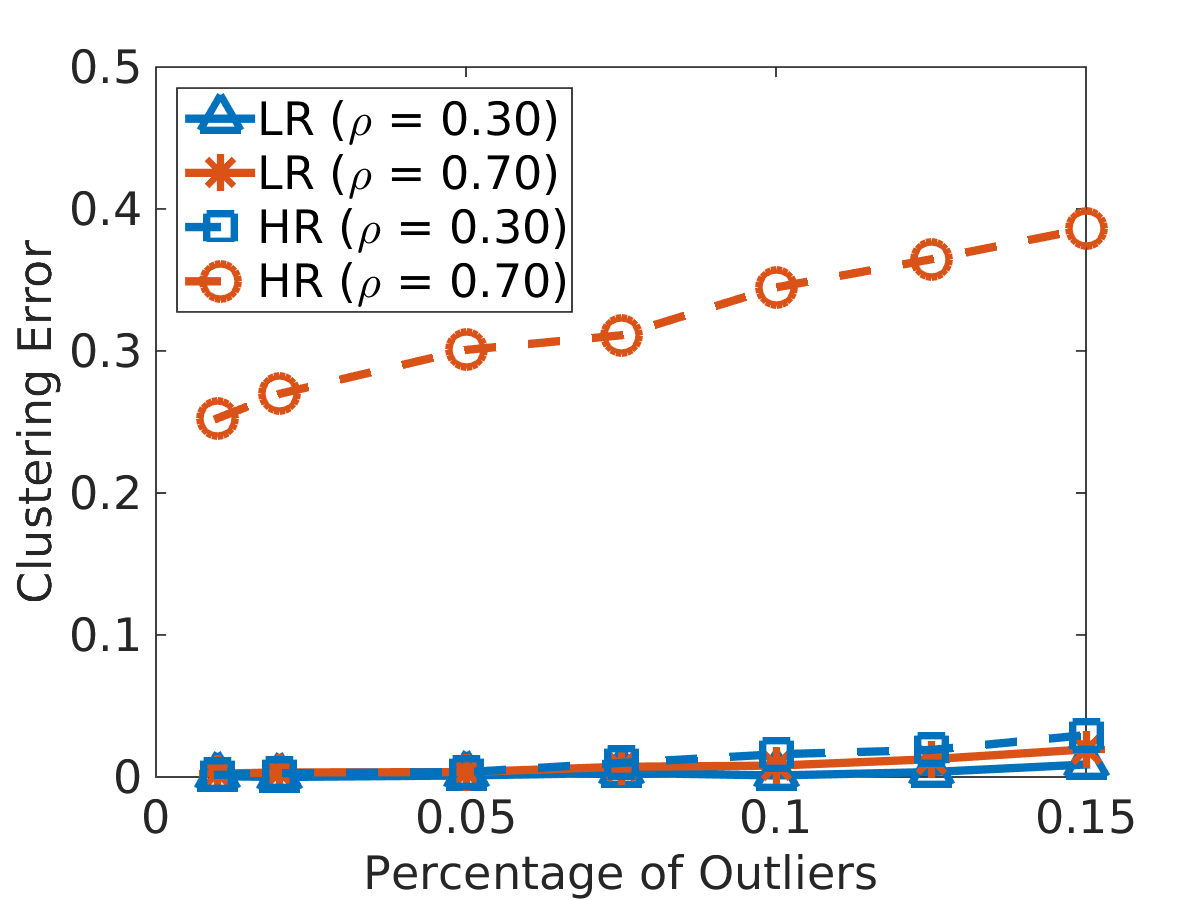
(d)

Figure 3: Noise and outliers’ impact in low-rank (LR) and high-rank (HR) data: (a) and (c) reconstruction error with added noise and outliers, respectively; (b) and (d) clustering error with added noise and outliers, respectively. LR: $K=3$, $d_{k}=5$,$D=50$, $N_{k}=50$; HR: $K=7$, $d_{k}=5$,$D=35$, $N_{k}=30$; $\rho\in\{0.30,0.70\}$.

To assess the robustness of our method to noise and corrupted entries, we generate low-rank and high-rank data (with range $[0,1]$) and add noise or outliers. We add gaussian noise with zero mean and standard deviation $\sigma$. To create outlying entries, we generate random values with uniform distribution, amplitude in $[0.2,1]$ and add them to a percentage of entries selected uniformly at random.

Figures 3a and 3b show, respectively, the reconstruction and clustering errors for added noise, as $\sigma$ increases in $[0.01,0.10]$. In the low-rank case, noise has no significant impact in the clustering performance up to $\sigma=0.10$. For high-rank with $30\%$ missing, the noise effect becomes evident after $\sigma=0.05$, while for $\rho=0.70$ the effect is much more meaningful. Figures 3c and 3d show the results for data corrupted with outliers in a percentage of entries going from $1\%$ to $15\%$. Although the reconstruction error evolves linearly with the percentage of outliers, its impact is significant. However, despite failing to recover the original data points, the clusters remain the same (even if the subspaces are different). Outliers only have a greater impact in the high-rank case with $\rho=0.70$.

4.2 Applications

In this section, we evaluate our method when applied to motion segmentation and motion capture problems. We show both qualitative and quantitative results.

4.2.1 Motion Segmentation

We consider the problem of motion segmentation, where we aim to cluster trajectories of feature points belonging to multiple objects in $F$ frames of a video sequence. Missing data in this context is frequent due to occlusion and failure in feature detection.

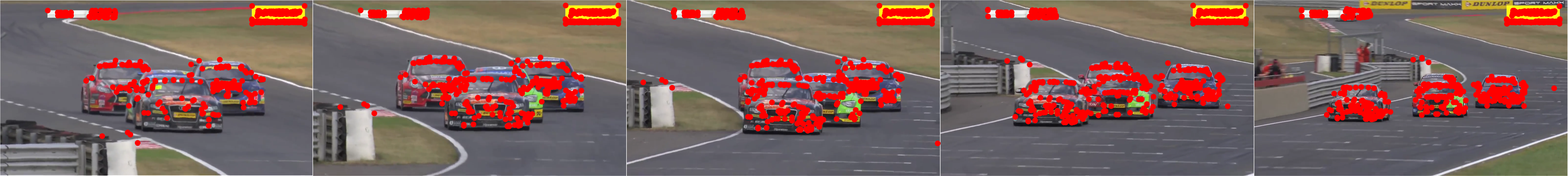
(a) Feature points.

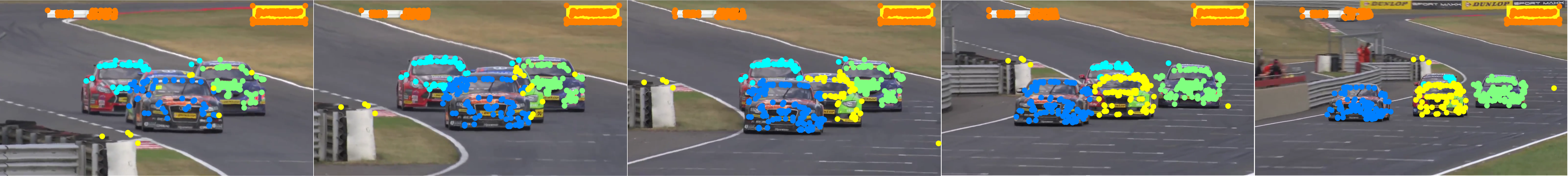
(b) Classified feature points.

Figure 4: Video sequence with 4 racing cars: (a) all feature points in red; (b) classified points, with one color per cluster.

First, we consider a sequence of 112 frames with 4 racing cars, from which we show 5 frames in Figure 4a. In this scenario, all cars aim to ride along the optimal path, having very similar motions (identical to a single object). However, in this sequence, after the curve and going for a long straight segment, they also change motion to try to overtake opponents, leading to occlusions. Moreover, feature point trackers are prone to errors and misdetections. For this experiment we use the Kanade-Lucas-Tomasi (KLT) algorithm [17, 21]. Despite these challenges, our method succeeds in grouping features from each car, Figure 4b. This experiment shows that our method is able to deal with similar subspaces (motion), occlusions and incomplete feature trajectories.

Next, we assess SSSA with the Hopkins 155 dataset, containing 155 sequences with 2 or 3 objects each. Since this dataset contains only complete trajectories, we add missing data as before, selecting uniformly at random with probability $\rho$ the set of entries corresponding to missing values. In this dataset the subspaces are affine, therefore, we add the constraint $\mathbf{1^{T}C=1^{T}}$ to problem (2).

Table 1: Reconstruction error for all the sequences in Hopkins 155 dataset. For each sequence in the dataset, we generate missing data at random for several $\rho$ with 20 trials each.

$\rho$	0.10	0.20	0.30	0.40	0.50	0.60	0.70	0.80
SSC-EWZF	0.070	0.101	0.133	0.183	0.253	0.351	0.481	0.654
SSSA	0.005	0.005	0.005	0.006	0.011	0.021	0.039	0.119

Table 2: Clustering error for all the sequences in Hopkins 155 dataset as a function of $\rho$. The results for the SSC-Lifting and MC-SSC are as reported in [9] and [31], respectively.

$\rho$	0.10	0.20	0.30	0.40	0.50	0.60	0.70	0.80
SSC-EWZF	0.180	0.204	0.226	0.245	0.257	0.275	0.296	0.318
MC-SSC	0.049	0.049	0.049	0.049	0.049	-	-	-
SSC-Lifting	0.024	0.025	0.022	0.023	0.028	0.033	0.033	-
SSSA	0.016	0.016	0.016	0.018	0.018	0.022	0.033	0.086

Table 1 shows the average reconstruction error in the 155 sequences for SSSA and SSC-EWZF. Table 2 shows the average clustering error for the same sequences. Here, we include SSC-Lifting, as reported by the author in [9]. In our experiments with the Hopkins data set, the MC algorithm did not converge with the parameters suggested by the authors. Thus, the results presented here for MC-SSC are the ones reported in [31]. For all levels of $\rho$, our method achieves the lowest errors.

The data of these sequences are low-rank, since we have 2 or 3 rigid objects and the dimension of each subspaces is at most $d=4$ in $D=2F\geq 28$. Therefore, to assess the performance in high-rank, we merge 6 sequences in one data matrix, with a total of 12 objects. Since each sequence has a different number of frames, we subsample the sequences into 10 frames ($D=20$), selecting frames from the original sequence as spread apart as possible. Figure 5 shows the first frame of each of these sequences and all the feature points from the $F$ frames.

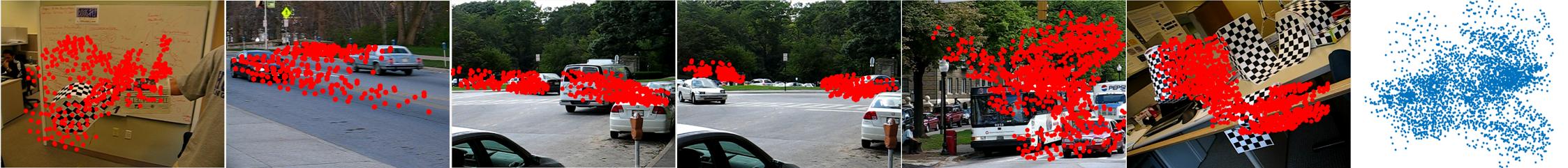
Figure 5: First frame of 6 sequences from the Hopkins 155 dataset. We build a data matrix with the trajectories of the objects from these sequences, in a total of 15 objects. The image on the right shows the points from the 15 objects in the same frame.

The right image plots all points in the same reference frame. Tables 3 and 4 show the errors for this high-rank case, where SSSA outperforms, as expected, the SSC-EWZF algorithm.

Table 3: Reconstruction error as a function of the missing rate, $\rho$, for a data matrix with 12 objects from 6 sequences from the Hopkins 155 dataset. We report the mean error of 20 trials for each $\rho$.

$\rho$	0.10	0.20	0.30	0.40	0.50	0.60	0.70	0.80
SSC-EWZF	0.065	0.145	0.223	0.313	0.415	0.537	0.663	0.791
SSSA	0.007	0.009	0.013	0.024	0.064	0.136	0.256	0.427

Table 4: Clustering error as a function of the missing rate, $\rho$, for a data matrix with 12 objects from 6 sequences from the Hopkins 155 dataset. We report the mean error of 20 trials for each level of $\rho$.

$\rho$	0.10	0.20	0.30	0.40	0.50	0.60	0.70	0.80
SSC-EWZF	0.236	0.301	0.343	0.430	0.505	0.601	0.680	0.769
SSSA	0.008	0.007	0.023	0.090	0.195	0.247	0.334	0.484

4.2.2 Motion Capture

We consider the motion capture problem, with the CMU Mocap dataset, where several sensors capture the motion of a human performing various activities. Each point in this dataset corresponds to the measurements of a sensor for a given frame. Here, we consider the completion and clustering for a sequence with 7 different activities. Similar to the Hopkins dataset and synthetic experiments, we generate missing data uniformly at random with probability $\rho$.

Table 5 shows the completion error. The results for SSC-Lifting are as reported by the author for the same sequence [9]. As before, the improvement achieved by SSSA is specially significant for higher values of $\rho$, where it achieves an error around three times lower than the other methods.

Since the sequence contains smooth transitions between the activities, the labeling is not unique. Therefore, we evaluate the clustering performance qualitatively. Figure 6a shows the labels for SSC (without missing data) and a set of frames from each activity. Without imposing any continuity constraint, as in [24], the clusters are temporally well defined. With $50\%$ missing data, using our method, there are small jumps in some clusters, see Figure 6b. Colored stars in Figure 6a highlight similar poses in different clusters. For example, red stars indicate frames from the drink class which are identical to frames in punch.

Table 5: Reconstruction error for a sequence of 7 activities (walk, squats, run, stretch, jumps, punches, and drinking) from the CMU Mocap dataset. The results for SSC-Lifting are as reported in [9]

$\rho$	0.10	0.20	0.30	0.40	0.50	0.60	0.70
SSC-EWZF	0.098	0.131	0.180	0.240	0.321	0.420	0.546
SSC-Lifting	0.089	0.125	0.170	0.213	0.285	0.430	0.590
SSSA	0.032	0.050	0.068	0.087	0.113	0.148	0.189

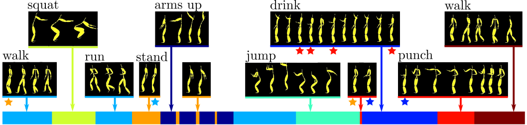
(a) Without missing data (SSC).

(b) SSSA with $50\%$ missing entries.

Figure 6: Clustering labels (one color per cluster) for the CMU Mocap dataset (subject 86, trial 2) and a subset of frames per activity: (a) without missing data (SSC); (b) with $\rho=0.50$ (SSSA).

5 Conclusions

We proposed a method for subspace segmentation with incomplete data lying in a union of affine subspaces. Subspace Segmentation by Successive Approximations is a method that recovers missing entries by exploiting the sparse representation of the data (for both observed and unobserved entries), constraining it to lie in the respective subspace. Using an iterative approach, we significantly improve the reconstruction and clustering performance. Extensive synthetic and real data experiments showed that our method dramatically outperforms current state of the art methods for both low and high-rank problems.

References

- [1] L. Balzano, A. Szlam, B. Recht, and R. Nowak. K-subspaces with missing data. In Statistical Signal Processing Workshop (SSP), 2012 IEEE, pages 612–615. IEEE, 2012.
- [2] S. Boyd, N. Parikh, E. Chu, B. Peleato, and J. Eckstein. Distributed optimization and statistical learning via the alternating direction method of multipliers. Foundations and Trends® in Machine Learning, 3(1):1–122, 2011.
- [3] R. Cabral, F. De la Torre, J. P. Costeira, and A. Bernardino. Unifying nuclear norm and bilinear factorization approaches for low-rank matrix decomposition. In Proceedings of the IEEE International Conference on Computer Vision, pages 2488–2495, 2013.
- [4] J.-F. Cai, E. J. Candès, and Z. Shen. A singular value thresholding algorithm for matrix completion. SIAM Journal on Optimization, 20(4):1956–1982, 2010.
- [5] E. J. Candes. The restricted isometry property and its implications for compressed sensing. Comptes Rendus Mathematique, 346(9-10):589–592, 2008.
- [6] E. J. Candes and Y. Plan. Matrix completion with noise. Proceedings of the IEEE, 98(6):925–936, 2010.
- [7] E. J. Candes, J. K. Romberg, and T. Tao. Stable signal recovery from incomplete and inaccurate measurements. Communications on pure and applied mathematics, 59(8):1207–1223, 2006.
- [8] A. P. Dempster, N. M. Laird, and D. B. Rubin. Maximum likelihood from incomplete data via the em algorithm. Journal of the royal statistical society. Series B (methodological), pages 1–38, 1977.
- [9] E. Elhamifar. High-rank matrix completion and clustering under self-expressive models. In Advances in Neural Information Processing Systems, pages 73–81, 2016.
- [10] E. Elhamifar and R. Vidal. Sparse subspace clustering. In Computer Vision and Pattern Recognition, 2009. CVPR 2009. IEEE Conference on, pages 2790–2797. IEEE, 2009.
- [11] E. Elhamifar and R. Vidal. Sparse subspace clustering: Algorithm, theory, and applications. IEEE transactions on pattern analysis and machine intelligence, 35(11):2765–2781, 2013.
- [12] B. Eriksson, L. Balzano, and R. D. Nowak. High-rank matrix completion. In AISTATS, pages 373–381, 2012.
- [13] A. Gruber and Y. Weiss. Multibody factorization with uncertainty and missing data using the em algorithm. In Computer Vision and Pattern Recognition, 2004. CVPR 2004. Proceedings of the 2004 IEEE Computer Society Conference on, volume 1, pages I–I. IEEE, 2004.
- [14] R. F. Guerreiro and P. M. Aguiar. Estimation of rank deficient matrices from partial observations: two-step iterative algorithms. In International Workshop on Energy Minimization Methods in Computer Vision and Pattern Recognition, pages 450–466. Springer, 2003.
- [15] R. Heckel and H. Bölcskei. Robust subspace clustering via thresholding. IEEE Transactions on Information Theory, 61(11):6320–6342, 2015.
- [16] W. Jiang, J. Liu, H. Qi, and Q. Dai. Robust subspace segmentation via nonconvex low rank representation. Information Sciences, 340:144–158, 2016.
- [17] B. D. Lucas, T. Kanade, et al. An iterative image registration technique with an application to stereo vision. 1981.
- [18] A. Y. Ng, M. I. Jordan, Y. Weiss, et al. On spectral clustering: Analysis and an algorithm. In NIPS, volume 14, pages 849–856, 2001.
- [19] D. Pimentel, R. Nowak, and L. Balzano. On the sample complexity of subspace clustering with missing data. In Statistical Signal Processing (SSP), 2014 IEEE Workshop on, pages 280–283. IEEE, 2014.
- [20] D. Pimentel-Alarcón, L. Balzano, R. Marcia, R. Nowak, and R. Willett. Group-sparse subspace clustering with missing data. In Statistical Signal Processing Workshop (SSP), 2016 IEEE, pages 1–5. IEEE, 2016.
- [21] J. Shi et al. Good features to track. In Computer Vision and Pattern Recognition, 1994. Proceedings CVPR’94., 1994 IEEE Computer Society Conference on, pages 593–600. IEEE, 1994.
- [22] M. Soltanolkotabi, E. J. Candes, et al. A geometric analysis of subspace clustering with outliers. The Annals of Statistics, 40(4):2195–2238, 2012.
- [23] M. Soltanolkotabi, E. Elhamifar, E. J. Candes, et al. Robust subspace clustering. The Annals of Statistics, 42(2):669–699, 2014.
- [24] S. Tierney, Y. Guo, and J. Gao. Segmentation of subspaces in sequential data. arXiv preprint arXiv:1504.04090, 2015.
- [25] M. E. Tipping and C. M. Bishop. Mixtures of probabilistic principal component analyzers. Neural computation, 11(2):443–482, 1999.
- [26] R. Vidal and P. Favaro. Low rank subspace clustering (lrsc). Pattern Recognition Letters, 43:47–61, 2014.
- [27] R. Vidal and R. Hartley. Motion segmentation with missing data using powerfactorization and gpca. In Computer Vision and Pattern Recognition, 2004. CVPR 2004. Proceedings of the 2004 IEEE Computer Society Conference on, volume 2, pages II–II. IEEE, 2004.
- [28] R. Vidal, Y. Ma, and S. Sastry. Generalized principal component analysis (gpca). IEEE Transactions on Pattern Analysis and Machine Intelligence, 27(12):1945–1959, 2005.
- [29] X. Wen, L. Qiao, S. Ma, W. Liu, and H. Cheng. Sparse subspace clustering for incomplete images. In Proceedings of the IEEE International Conference on Computer Vision Workshops, pages 19–27, 2015.
- [30] Z. Wen, W. Yin, and Y. Zhang. Solving a low-rank factorization model for matrix completion by a nonlinear successive over-relaxation algorithm. Mathematical Programming Computation, pages 1–29, 2012.
- [31] C. Yang, D. Robinson, and R. Vidal. Sparse subspace clustering with missing entries. In Proceedings of the 32nd International Conference on Machine Learning (ICML-15), pages 2463–2472, 2015.