Disordered Quantum Spin Chains with Long-Range Antiferromagnetic Interactions

Abstract

We investigate the magnetic susceptibility $\chi(T)$ of quantum spin chains of $N=1280$ spins with power-law long-range antiferromagnetic couplings as a function of their spatial decay exponent $\alpha$ and cutoff length $\xi$. The calculations are based on the strong disorder renormalization method which is used to obtain the temperature dependence of $\chi(T)$ and distribution functions of couplings at each renormalization step. For the case with only algebraic decay ($\xi=\infty$) we find a crossover at $\alpha^{*}=1.066$ between a phase with a divergent low-temperature susceptibility $\chi(T\rightarrow 0)$ for $\alpha>\alpha^{*}$ to a phase with a vanishing $\chi(T\rightarrow 0)$ for $\alpha<\alpha^{*}$. For finite cutoff lengths $\xi$, this crossover occurs at a smaller $\alpha^{*}(\xi)$. Additionally we study the localization of spin excitations for $\xi=\infty$ by evaluating the distribution function of excitation energies and we find a delocalization transition that coincides with the opening of the pseudo-gap at $\alpha_{c}=\alpha^{*}$.

The magnetic susceptibility of doped semiconductors such as P-doped Si is known to diverge at low temperature with an anomalous power lawloehneysen . This can be taken as evidence for local magnetic moments, formed in localized states due to interactions pwanderson0 ; pwanderson ; mott ; finkelsteinesr , that are positioned randomly, and coupled by exchange interactions andres ; bhattlee ; bhattreview ; milovanovic , as illustrated in Fig. 1. At low dopant density $n_{\rm D}$ these magnetic moments are coupled weakly by the antiferromagnetic exchange interaction $J$ between the hydrogen-like dopant levels andres ; bps . For $n_{\rm D}\ll 1/a_{B}^{3},$ where $a_{B}$ is the Bohr radius of the dopants, the magnetic susceptibility is observed to follow the Curie law $\chi\sim 1/T$ of free magnetic momentsandres ; sarachik ; lakner . However, as the density of dopants is increased, the magnetic susceptibility diverges like $\chi\sim T^{-\alpha_{m}}$ with a decreasing anomalous power $\alpha_{m}<1.$ This has been indentified as being a consequence of a random distribution of exchange couplings due to the random positions of dopants bhattrice ; rosso . Indeed, in Ref. bhattlee, it was argued that such random antiferromagnetically coupled $S=1/2$ spins form a ground state of hierarchically coupled singlets, the random singlet phase. The random distribution of excitation energies leads to a temperature dependent concentration of free magnetic moments $n_{\rm FM}(T),$ resulting in an anomalous power $\alpha_{m}<1$.

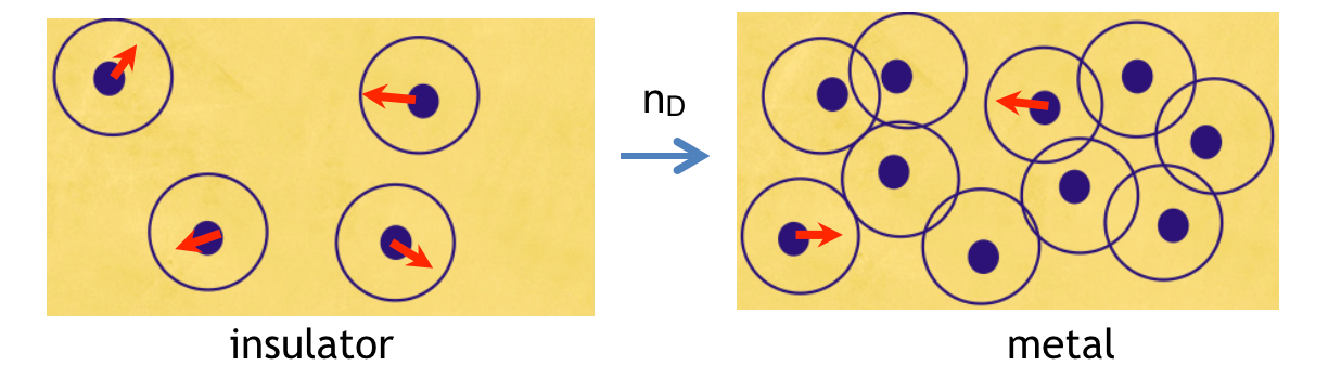
Figure 1: Left: Sketch of electronic orbitals at low doping concentration $n_{\rm D}$. All states are localized and magnetic, as indicated by red arrows. Right: At larger $n_{\rm D}$ states at Fermi energy are delocalized, coexisting with localized magnetic states.

With increasing doping concentration the density of magnetic moments is observed to decrease. Surprisingly, both magnetic susceptibility and specific heat measurements indicate that there remains a finite density of magnetic moments at the metal-insulator transition loehneysen . In P:Si about 10% of all dopants are magnetic at the metal-insulator transition (MIT) loehneysen . These moments can be created from localized states in the tail of the band with onsite interactions mott ; milovanovic , or they may be created due to an instability of the disordered Fermi liquid with long-range interactions finkelsteinesr . At the same time, the power $\alpha_{m}$ of the divergence of the magnetic susceptibility is experimentally observed to converge to a constant value as the doping concentration is increased beyond the MIT (in Si:P $\alpha_{m}\rightarrow.64$ sarachik , $\alpha_{m}\rightarrow.62$ bps and $\alpha_{m}\rightarrow.5$ lakner ; loehneysen ). This situation has been modeled by a phenomenological two-fluid model andres ; bhattlee ; paalanen ; sachdev . It presumes that the antiferromagnetic interaction between localized magnetic moments is dominant even in the metallic phase, leading to the formation of a random singlet phase.

On the metallic side of the transition the indirect exchange interaction $J_{ij}$ becomes long-ranged, mediated by the itinerant electrons RKKY . The typical value of this RKKY coupling $J_{ij}$ decays with a power law with exponent $\alpha=d$, oscillating in sign with a period equal to the Fermi wavelength $\lambda_{F}$. Its amplitude is widely, log-normally distributed lerner .

Thus, aiming to get a better understanding of the magnetic properties of doped semiconductors, we consider the Hamiltonian of $N$ long range interacting $S=1/2$ spins,

$$H=\sum_{i\neq j,\beta}J_{ij}^{\beta}S_{i}^{\beta}\,S_{j}^{\beta},$$ (1)

randomly placed on a periodic lattice of length $L$ and lattice spacing $a$. We assume that the couplings between all pairs of sites $i,j,$ are antiferromagnetic decaying as

$$J_{ij}^{\beta}=J|({\bf r}_{i}-{\bf r}_{j})/a|^{-\alpha}\exp(-|{\bf r}_{i}-{\bf r}_{j}|/\xi),$$ (2)

which is cut off exponentially by the length scale $\xi$, allowing us to tune between the limit of short-ranged coupled spins for small $\xi\rightarrow L/N^{1/d},$ and the long-range RKKY-type coupling as $\xi\rightarrow\infty$ footnote1 .

Random Spin Chains.–

While the situation in three-dimensional systems for experimentally accessible temperatures has been at least semi-quantitatively explained, the generation of ferromagnetic bonds at intermediate stages in three-dimensions bhattlee has made understanding the asymptotic low-energy (low-temperature) behavior not feasible.

Therefore, we focus here on the study of random spin chains with long range interactions modeled by Eq. (1). From a numerical perspective, the one-dimensional models offer the possibility of exploring larger length scales, and hopefully clearer asymptotic behavior. It is well known that in one-dimensional models with power-law hopping fyodorov1996 ; zhou , as well as power-law correlated disorder moura ; izraelev , an Anderson localization-delocalization transition is found for non-interacting electrons which has critical properties similar to the ones observed in the three dimensional Anderson model leeramak ; eversmirlin . Thus, one expects also a delocalization transition in random spin chains with long range interactions, as recently observed in Ref. ours, . Moreover, it is well known that many aspects of higher dimensional short ranged models can be captured in one-dimension by considering longer ranged interactions. Consequently, e.g., in classical spin models of ferromagnets as well as spin glasses with random ferromagnetic and antiferromagnetic bonds KotliarAndersonStein ; bhattyoung , there is a clear correspondence between the power law exponent ($\alpha$) of the one-dimensional model with the dimensionality of the higher dimensional system regarding their critical behavior.

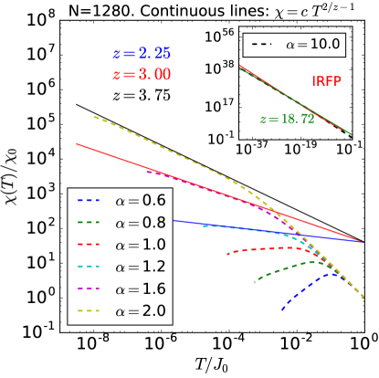
Figure 2: Magnetic susceptibility of a chain with $N=1280$ randomly placed spins, interacting via antiferromagnetic long-range couplings $J_{ij}^{x}$, given by Eq. (2), with chain length $L/a=100N$, and $\alpha=0.6,\dots,2.0$. The cutoff length is set to $\xi=\infty$.The susceptibility is normalized to its value at $T=J_{0}$. The continuous lines represent fits to $\chi\sim T^{2/z-1}$ with finite $z$ at low temperatures and support our argument that our model does not flow to the IRFP. The inset shows the susceptibility for $\alpha=10.0$ along with the power law with $z=18.72$ (green line) and the IRFP result (red line).

The magnetic susceptibility at low temperatures is determined by the concentration of free paramagnetic moments $n_{FM}(T)$ (we set $k_{B}=1$) bhattlee ,

$$\chi(T)\propto\frac{n_{FM}(T)}{T}=\frac{n_{M}}{T}\,\int_{0}^{T}d\epsilon\,\rho(\epsilon),$$ (3)

where $n_{M}$ is the total density of magnetic moments in the chain, and $\rho(\epsilon)$ the density of states of spin excitations with energy $\epsilon$.

In order to compute $n_{FM}(T)$ numerically, we apply the strong-disorder renormalization group (SDRG) procedure bhattlee ; dasguptama ; fisher2 , choosing the pair with largest coupling $(l,m)$ which in its ground state forms a singlet. Taking the expectation value of the Hamiltonian in that singlet state and performing second-order perturbation theory in the coupling between all spins and the spins of that singlet pair bhattlee ; dasguptama ; fisher ; fisher2 ; sigrist ; monthus , we obtain renormalized couplings between spins $(i,j)$ ours ,

$$(J^{x}_{ij})^{\prime} = J_{ij}^{x}-\frac{(J^{x}_{il}-J^{x}_{im})(J^{x}_{lj}-J^{x}_{mj})}{J^{x}_{lm}+J^{z}_{lm}},$$

$$(J_{ij}^{z})^{\prime} = J^{z}_{ij}-\frac{(J^{z}_{il}-J^{z}_{im})(J^{z}_{lj}-J^{z}_{mj})}{2J^{x}_{lm}}.$$ (4)

We implement the SDRG monthus by iterating these RG rules for each realization of bare coupling parameters until the system has reached the energy $\Omega=T$. We then record the number of remaining spins which have not yet formed a singlet, obtaining the density $n_{FM}(T)$ bhattlee . We resort to numerical iteration with a large number ($\sim$20 000) of random realizations needed for reliable statistics.

In Fig. 2 we show numerical results for the susceptibility of the long-ranged, $\xi=\infty$, XX-spin chain. Note that the lowest temperature scale that can be reached for the finite system size $L$ is of the order of $T_{min}=J_{min}/k_{\rm B}=J_{0}(L/2a)^{-\alpha}$, which is why the data for different values of $\alpha$ terminate at different values of $T/J_{0}$. At low temperatures, we can see a power law behavior, which appears linear on a double logarithmic scale, consistent with a finite dynamical exponent $z$. We note that in each RG step, a fraction $dn_{FM}/n_{FM}(\Omega)$ of the remaining spins at renormalization energy $\Omega=\text{max}(J)$ are taken away. Since this is due to the formation of a singlet with coupling $J=\Omega$, this fraction should equal $2P(J=\Omega,\Omega)d\Omega$, leading to the differential equation

$$\frac{dn_{FM}}{d\Omega}=2\,P(J=\Omega,\Omega)\,n_{FM}(\Omega),$$ (5)

where $P(J,\Omega)$ is the probability distribution of couplings $J$ at a given renormalization energy $\Omega$ fisher2 . At the IRFP this distribution is known to be given by

$$P(J,\Omega)=(J/\Omega)^{1/z-1}/(z\Omega),$$ (6)

with the dynamical exponent $z=\ln(\Omega_{0}/\Omega)$ for initial renormalization energy $\Omega_{0}$. Then, the solution of Eq. (5) is $n_{FM}(\Omega)=1/\ln^{2}(\Omega_{0}/\Omega),$ which yields the IRFP magnetic susceptibility $\chi(T)\sim 1/(T\ln^{2}(T))$ via Eq. (3) fisher2 . However, if the dynamical exponent $z$ is finite and fixed, the solution of Eq. (5) in conjunction with Eq. (3), gives rise to a power law behavior for the low temperature susceptibility of the form

$$\chi(T)\sim T^{2/z-1},$$ (7)

consistent with our numerical results shown in Fig. 2 for $z=z(\alpha)$, a monotonically increasing function of $\alpha$ that can be extracted by linear regression fits of the susceptibility in a logarithmic scale (continuous lines). If $z>2$, the magnetic susceptibility diverges as $T\rightarrow 0,$ with an anomalous power $\alpha_{m}=1-2/z<1$ that also grows with $\alpha$. In the region $z<2$, this power becomes negative and we have a vanishing susceptibility at zero temperature, consistent with the formation of a pseudo-gap in the density of sates. A similar behavior has been observed previously in Refs. bhattlee, and bhattdiscussions, . The crossover value $z=2$, where the susceptibility saturates to a constant, occurs at a given $\alpha=\alpha^{*}$, which from Fig. 2 can be concluded to be somewhere between $1.0$ and $1.2$. Assuming a linear dependence on $\alpha$ of the form

$$z=\frac{2-b}{\alpha*}\alpha+b,$$ (8)

we find this crossover value to be $\alpha^{*}=1.066\pm 0.002$ by a linear regression fit of $z(\alpha)$ as shown in Fig. 3 (dashed black line), where the error only includes the fitting uncertainty. All values of $z$ used for the fit are found by fitting the low temperature susceptibility curves to Eq. (7) as it is done in Fig. 2 for $\alpha=1.2,1.6$, and $2.0$.

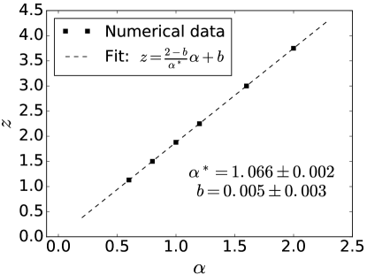
Figure 3: Dynamical exponent $z$ extracted by fitting the low-temperature susceptibility in Fig. 2 to Eq. (7) as a function of the power $\alpha$ (squares). These numerical results are then fit to Eq. (8) (dashed line), which allows us to extract the crossover value $\alpha^{*}=1.066\pm 0.002$.

The inset in Fig. 2 displays the susceptibility for $\alpha=10.0$, along with the curve given by Eq. (7) with the value $z=18.72$ predicted by Eq. (8), together with the IRFP magnetic susceptibility. We can see clearly a better agreement of the numerical results with the finite $z$ curve, indicating the flow to a finite $z$ fixed point and not to the IRFP, as it occurs for nearest neighbor interactions.

We note that at very large $\alpha\gg 10$ we find a finite number of free moments even at the smallest renormalization energies which are accessible in the finite spin chain. In our model, spins are randomly placed in a very diluted lattice, a situation in which nearest neighbor distances bigger than one lattice spacing $a$ is highly probable. Therefore, at very large values of $\alpha$, given the power law nature of the coupling stregths, one starts with an initial distribution $P(J)$ heavily wighted near $J=0$, which might explain the above mentioned residual free moments. A thorough exploration of this important $\alpha\gg 10$ limit is left for future studies.

Another way to investigate whether or not there is at finite $\alpha$ a strong disorder fixed point with a finite dynamical exponent $z(\alpha)$ or a transition to the IRFP at a specific finite power $\alpha_{IR}$ is to numerically inspect the evolution of the width of the couplings probability distribution with the RG flow. At the IRFP, this distribution, according to Eq. (6), gets wider at every RG step, i.e., $W=(\langle\ln(J/\Omega_{0})^{2}\rangle-\langle\ln(J/\Omega_{0})\rangle^{2})^{1/2}=z(\Omega)=\ln(\Omega_{0}/\Omega)$ increasing monotonically as $\Omega$ is lowered during the RG flow. However, as shown in Fig. 4, our system does not follow this trend for $\alpha\gg 1$ (see inset). Instead, the width is found to saturate to a constant value after a non-monotonic transient behavior, which is a strong indication of a finite $z$ fixed point. It is worth noting, that given the large number of couplings present in our system ($N(N-1)/2$ before any renormalization is performed), we have only picked the largest coupling to every spin $J_{1}$ in order to calculate $P(J),$ denoting the width of this approximate distribution by $W_{1}$.

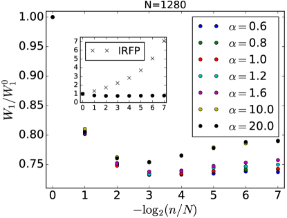
Figure 4: Width $W_{1}$ of the distribution function of nearest-neighbor couplings as a function of the fraction of remaining spins. The negative logarithmic in base two is used to have an equally spaced horizontal variable that grows as the number of spins decreases. All values have been normalized by the width $W_{1}^{0}(\alpha)$ of the initial distribution and the parameters are kept as in Fig. 2. Inset: $W_{1}/W_{1}^{0}$ for a simple nearest neighbor model with uniformly distributed couplings (crosses) know to flow to the IRFP. The numerical results for $\alpha=20.0$ (black circles) are included for comparison purposes.

In a previous study of the $\xi=\infty$ limit, we found evidence for a delocalization transition of spin excitations at a critical power $\alpha_{c}$ by examining the distribution function of the lowest excitation energy from the ground state of long-range coupled random spin chains (N=128) ours . At $\alpha=\alpha_{c}$, this gap distribution was observed to coincide with a critical function, separating a phase with localized excitations at large $\alpha>\alpha_{c}$, where the distribution is Poissonian, from a phase with extended excitations at small $\alpha<\alpha_{c}$, where the gap distribution follows the Wigner surmise footnote2 . Since in our present study we find strong evidence in $\chi(T)$ that the density of states of spin excitations presents a pseudogap for $\alpha<\alpha^{*}$, we revisit the gap distribution function to check if the delocalization of spin excitations at $\alpha_{c}$ coincides with $\alpha^{*}$. Following the procedure carried out in Ref. ours, , we now place spins randomly on the sites of a lattice with lattice constant $a$, as done in the calculation of the susceptibility above, and study the distribution of excitation energies.

Before proceeding, it is worthwhile to recall the results of Refs. fisheryoung, ; juhasz, , where the distribution of excitation gaps $\epsilon_{1}$ from the ground state was derived for the random transverse Ising model. Since the probability to find a gap $\epsilon_{1}$ is proportional to the number of remaining spins $N_{FM}=n_{FM}(\Omega)L$, at RG energy $\Omega$, the distribution function of the lowest excitation energy $\epsilon_{1}$ equal to the energy scale of the last RG step was derived by a scaling argument. Using the same argument for our model we obtain that the distribution of the excitation energies $\epsilon_{1}$ should have the form of a Weibull function juhasz ; weibull ,

$$P_{W}(\epsilon_{1})=\frac{2u_{0}^{2/z}L}{z}\epsilon_{1}^{2/z-1}\exp(-(u_{0}\epsilon_{1})^{2/z}L),$$ (9)

where $u_{0}$ is a constant. The average excitation energy scales with system size $L$ as $\langle\epsilon_{1}\rangle=\frac{\Gamma(1+z/2)}{u_{0}}L^{-z/2}.$ Since delocalization causes level repulsion, Eq. (9) yields a delocalization transition when $z(\alpha)<z_{c}=2.$ Thus, if this scaling scheme of the strong disorder RG holds at the delocalization transitions, we conclude that $z_{c}=2=z^{*}$ which means that the first appearance of a pseudogap coincides with the delocalization transition.

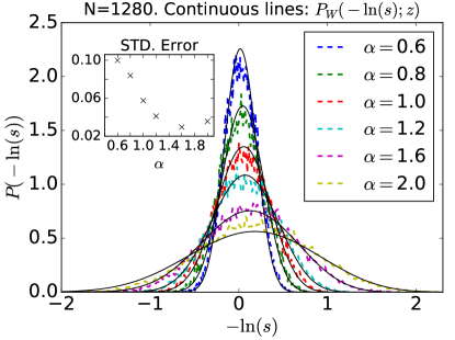
Figure 5: Distribution of the lowest excitation gap $\epsilon_{1}$ scaled by its mean value, $s=\epsilon_{1}/\langle\epsilon_{1}\rangle$, for $\xi=\infty$ and $\alpha=0.6,0.8,\dots,2.0$. The remaining parameters are as in Fig. 2.

In Fig. 5 we show the distribution function of the lowest excitation energy $\epsilon_{1}$ using the logarithmic variable $x=-\ln\left(\epsilon_{1}/\langle\epsilon_{1}\rangle\right)$ in the limit of long-range interaction, i.e., $\xi=\infty$. The continuous black curves correspond to the fits to the Weibull distribution in Eq. (9) multiplied by the cutoff function introduced in Ref. ours, , $\exp(c/(x-x_{max}))$, which is introduced in order to account for the fact that at finite size $L$ with periodic boundary conditions we have a maximum value $x_{max}=-\ln(\epsilon_{min}/\Delta(\alpha))$ arising from the minimal energy scale $\epsilon_{min}=(1/2)\,J_{0}\,(L/6a)^{-\alpha}$. Here, the factor 6 is included since the numerical data is obtained in the third to last RG step. That way we tried to minimize the effect of that sharp cutoff due to the finite size of the system. We found $c=16$ to work for all fits independent of the value of $\alpha$, while $u_{0}$ was freely changed for each curve. Given the good quality of the fits and the fact that we used the values of $z(\alpha)$ obtained from the fitting of the susceptibility data as plotted in Fig. 3, we can conclude that indeed, the delocalization transition occurs at the same value at which the pseudogap appears, i.e., $\alpha_{c}=\alpha^{*}=1.066\pm 0.002$.

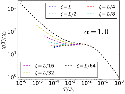
Figure 6: Log-Log plot of the magnetic susceptibility for $\alpha=d=1$ and $\xi/L=1,1/2,\dots,1/64$. The remaining parameters are kept as in Fig. 2, and the susceptibility is rescaled in the same manner.

As the power $\alpha=d=1$ corresponds to the typical decay of the RKKY coupling in a 1D electron system in the metallic regime, we may conclude from the results in Fig. 2 that the magnetic susceptibility due to the randomly coupled magnetic moments decays to zero in the metallic regime. Turning on a finite cutoff $\xi,$ as caused by the finite electron localization length when the magnetic moments are surrounded by an electronic system, we see in Fig. 6 that the magnetic susceptibility diverges for $\xi<L/4.$ At low temperatures we observe a power law behavior indicating a finite $z$ fixed point. Increasing the cutoff to $\xi>L/4$ we observe in Fig. 6 a low-temperature suppression of the magnetic susceptibility, clearly demonstrating the opening of a pseudogap as the range of the interaction increases.

For fixed small $\xi=L/32$ we observe in Fig. 7 that at sufficiently low temperatures the magnetic susceptibility recovers the power law divergence consistent with finite $z>2$, after some transient behavior. As expected, due to the presence of a finite $\xi$, this divergence is faster for every $\alpha$ when compared to the pure power-law couplings model, i.e., $z(\alpha,\xi=L/32)>z(\alpha,\xi=\infty)$. In fact, for $\alpha=0.6,0.8,$ and $1.0$, we still observe for finite $\xi$ a divergence in $\chi(T)$, in contrast with the results shown in Fig. 2 for $\xi=\infty$, where for these values of $\alpha$ we find $z(\alpha)<2$ corresponding to a pseudogap.

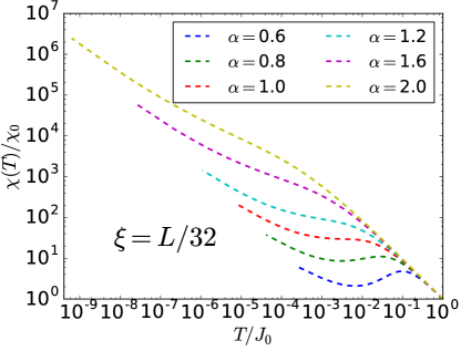
Figure 7: Logarithmic plot of the susceptibility for a fixed and finite cutoff length $\xi=L/32$ and $\alpha=0.6,0.8,\dots,2.0$. The remaining parameters are kept as in Fig. 2.

In conclusion, we derived the temperature dependence of the magnetic susceptibility of quantum spin chains with power-law long-range antiferromagnetic couplings as function of the exponent $\alpha$ and the cutoff length $\xi$. We identified a crossover between a phase with a divergent low-temperature magnetic susceptibility to a phase with a vanishing low-temperature susceptibility at a critical $\alpha^{*}$. For finite cutoff lengths $\xi$, this crossover occurs at smaller values $\alpha^{*}(\xi)<\alpha^{*}$. We also explored the localization of spin excitations in the limit $\xi=\infty$, by computing the distribution functions of renormalized couplings and identified a delocalization transition at $\alpha_{c}$, which turns out to coincide with $\alpha^{*}$.

In order to analyze experimental results in doped bulk semiconductors the study of higher-dimensional random spin systems with long-range couplings is needed. However, in higher dimensions it is known that even if the initial distribution is purely antiferromagnetic, ferromagnetic couplings can be generated upon renormalization sigrist . This is expected to modify strongly the temperature dependence of the magnetic susceptibility. Furthermore, as the density of itinerant electrons increases with the doping concentration the indirect exchange coupling competes with the Kondo effect which screens the local moments with the itinerant electron spins. Indeed, on the metallic side of the transition in P:Si there are indications of Kondo correlations in thermopower measurements schlager . It has been shown that the Kondo temperature $T_{K}$ is widely distributed in the vicinity of the AMIT, which results in a power law divergence of the magnetic susceptibility bhatt92 ; langenfeld ; dobros ; cornaglia ; kats . Its power $\alpha$ has been related to multifractal correlations, yielding in $d=3$ dimensions with the multifractality parameter $\alpha_{0}$, $\alpha=2-\alpha_{0}/3=.651(.652,.650)$ kats , which happens to be close to the experimentally observed value lakner ; bps ; sarachik ; loehneysen . It remains a challenge to study the effect of the interplay of both the long range exchange couplings and the Kondo couplings on the low temperature magnetic properties.

This research has been supported by DFG KE-15 Collaboration grant. H.Y. Lee acknowledges support from MEXT as Exploratory Challenge on Post-K computer (Frontiers of Basic Science: Challenging the Limits). S. Haas acknowledges funding by DOE Grant Number DE-FG02-05ER46240 and would also like to thank the Humboldt Foundation for support. R. N. Bhatt acknowledges support from DOE Grant No. DE-SC0002140, and during the writing of the manuscript, the hospitality of the Aspen Center for Physics.

Computation for the work described in this paper was supported by the University of Southern California’s Center for High-Performance Computing (hpc.usc.edu).

References

- (1) *
- (2) H. v. Löhneysen, Adv. in Solid State Phys. 40, 143 (2000).
- (3) P. W. Anderson, Phys. Rev. 109, 1492 (1958).
- (4) P. W. Anderson, Nobel Lectures in Physics 1980, 376 (1977).
- (5) N. F. Mott, J. Phys. Colloques 37, C4 (1976).
- (6) A. M. Finkel’shtein, JETP Lett. 46, 513 (1987).
- (7) R. N. Bhatt, P. A. Lee, Phys. Rev. Lett. 48, 344 (1982).
- (8) R. N. Bhatt, Physica Scripta T14, 7 (1986).
- (9) M. Milovanovic, S. Sachdev, and R. N. Bhatt, Phys. Rev. Lett. 63, 82 (1989).
- (10) K. Andres, R. N. Bhatt, P. Goalwin, T. M. Rice, and R. E. Walstedt, Phys. Rev. B 24, 244260 (1981) .
- (11) R. N. Bhatt, M. Paalanen, S. Sachdev, J. de Phys. Coll. C8, 49 (1988).
- (12) M. P. Sarachik, A. Roy, M. Turner, M. Levy, D. He, I. L. Isaacs and R. N. Bhatt, Phys. Rev. B 34, 387 (1986).
- (13) M. Lakner and H. v. Löhneysen, Phys. Rev. Lett. 70, 3475 (1993).
- (14) R. N. Bhatt and T. M. Rice, Philos. Nag. 8 42, 859 (1980).
- (15) S.M. Rosso, Phys. Rev. Lett. 44, 1541 (1980).
- (16) M. A. Paalanen, J. E. Graebner, R. N. Bhatt, and S. Sachdev, Phys. Rev. Lett. 61, 597 (1988).
- (17) S. Sachdev, Phys. Rev. B 39, 5297 (1989).
- (18) M. A. Ruderman and C. Kittel, Phys. Rev. 96, 99 (1954); T. Kasuya, Prog. Theor. Phys. 16, 45 (1956); K. Yosida, Phys. Rev. 106, 893 (1957).
- (19) I. V. Lerner, Phys. Rev. B 48, 9462 (1993).
- (20) In this work we restrict ourselves to the case of power-law decaying couplings without alternating sign. Inclusion of the sign alternation will likely lead to different fixed points of mixed character, such as discussed in E. Westerberg, A. Furusaki, M. Sigrist, and P. A. Lee, Phys. Rev. B 55, 12578 (1997).
- (21) A. D. Mirlin, Y. V. Fyodorov, F.-M. Dittes, J. Quezada, T. H. Seligman, Phys. Rev. E 54, 3221 (1996).
- (22) C. Zhou and R. N. Bhatt, Phys. Rev. B 68, 045101 (2003).
- (23) F. de Moura and M. L. Lyra, Phys. Rev. Lett. 81, 3735 (1998); Physica A 266, 465 (1999).
- (24) F. M. Izraelev and A. A. Krokhin, Phys. Rev. Lett. 82, 4062 (1999).
- (25) P. A. Lee and T. V. Ramakrishnan, Rev. Mod. Phys. 57, 287 (1985).
- (26) F. Evers and A. Mirlin, Rev. Mod. Phys. 80, 1355 (2008).
- (27) N. Moure, S. Haas and S. Kettemann, Europhys. Lett. 111, 27003 (2015).
- (28) G. Kotliar, P. W. Anderson, and D. L. Stein, Phys. Rev. B 27, 602(R) (1983).
- (29) R. N. Bhatt and A. P. Young, Journal of Magnetism and Magnetic Materials 54-57, 191 (1986).
- (30) C. Dasgupta, S.-K. Ma, Phys. Rev. B 22, 1305 (1980).
- (31) D. S. Fisher, Phys. Rev. B 50, 3799 (1994).
- (32) D. S. Fisher, Phys. Rev. Lett. 69, 534 (1992).
- (33) E. Westerberg, et al., Phys. Rev. B 55, 12578 (1997); Phys. Rev. Lett. 75, 4302 (1995).
- (34) F. Igloi, C. Monthus, Phys. Rep. 412, 277 (2005).
- (35) R. Bhatt, unpublished (1982).
- (36) We note that these fitting functions had to be multiplied by a cutoff distribution of the form (), where , to account for the finite size of the system giving rise to a minimum excitation energy of the order of (), where is the average excitation gap.
- (37) D. S. Fisher, A. P. Young, Phys. Rev. B 58, 9131 (1998).
- (38) R. Juhasz and Y.-C. Lin, F. Igloi, Phys. Rev. B 73, 224206 (2006).
- (39) Papoulis, Athanasios Papoulis; Pillai, S. Unnikrishna. Probability, Random Variables, and Stochastic Processes (4th ed.). Boston: McGraw-Hill (2002).
- (40) H. Schlager, and H. Löhneysen, Europhys. Lett. 661 (1997).
- (41) R. N. Bhatt and D. S. Fisher, Phys. Rev. Lett. 68, 3072 (1992).
- (42) A. Langenfeld and P. Wölfle, Ann. Physik 4, 43 (1995).
- (43) V. Dobrosavljevic, T. R. Kirkpatrick, and G. Kotliar, Phys. Rev. Lett. 69, 1113 (1992); E. Miranda, V. Dobrosavljevic, and G. Kotliar, ibid. 78, 290 (1997).
- (44) P. S. Cornaglia, D. R. Grempel, and C. A. Balseiro, Phys. Rev. Lett. 96, 117209 (2006).
- (45) S. Kettemann, E. R. Mucciolo, and I. Varga, Phys. Rev. Lett.103, 126401, (2009); S. Kettemann, E. R. Mucciolo, I. Varga, K. Slevin, Phys. Rev. B 85, 115112 (2012).