Common factors, trends, and cycles
in large datasets

Abstract

This paper considers a non-stationary dynamic factor model for large datasets to disentangle long-run from short-run co-movements. We first propose a new Quasi Maximum Likelihood estimator of the model based on the Kalman Smoother and the Expectation Maximisation algorithm. The asymptotic properties of the estimator are discussed. Then, we show how to separate trends and cycles in the factors by mean of eigenanalysis of the estimated non-stationary factors. Finally, we employ our methodology on a panel of US quarterly macroeconomic indicators to estimate aggregate real output, or Gross Domestic Output, and the output gap.

JEL classification: C32, C38, C55, E0.

Keywords: Non-stationary Approximate Dynamic Factor Model; Trend-Cycle Decomposition; Quasi Maximum Likelihood; EM Algorithm; Kalman Smoother; Gross Domestic Output; Output Gap.

1 Introduction

This paper is about two stylized facts of macroeconomic time series: co-movements and non-stationarity (Lippi and Reichlin, 1994a). More precisely, this paper is about disentangling long-run co-movements (common trends) from short-run co-movements (common cycles) in a large dataset of non-stationary US macroeconomic indicators.

Since the seminal work of Beveridge and Nelson (1981), the issue of decomposing GDP into a trend and a cycle has been a central question in both time series econometrics and policy analysis. This is not surprising, as long-run trends are mainly influenced by supply-side factors, while short-run cycles are mainly associated with demand-side factors, and therefore different estimates of the trend and of the cycle can lead to different policy recommendations. Given the relevance of the issue, in the last 30 years, many papers have suggested different ways to obtain a Trend-Cycle (TC) decomposition of GDP. Roughly speaking, those works can be grouped under two main approaches: one based on univariate methods (e.g. Watson, 1986; Lippi and Reichlin, 1994b; Morley et al., 2003; Dungey et al., 2015), and another using multivariate, but low-dimensional, time series techniques (e.g. Stock and Watson, 1988; Lippi and Reichlin, 1994a; Gonzalo and Granger, 1995; Garratt et al., 2006; Creal et al., 2010).

In this paper we use a novel approach to decompose GDP into a trend and cycle based on large datasets. We first disentangle common and idiosyncratic dynamics by using a Non-Stationary Approximate Dynamic Factor Model (DFM), and then we disentangle common trends from common cycles by applying a non-parametric TC decomposition to the latent common factors. Our methodology builds on four points: first, focusing on a high-dimensional setting is crucial, as only in a high-dimensional setting it is possible to disentangle common from idiosyncratic dynamics in a consistent way (Forni et al., 2000; Bai and Ng, 2002; Stock and Watson, 2002) — i.e., we can separate macroeconomic fluctuations from sectoral dynamics and measurement error only in a high-dimensional setting. Second, assuming the existence of a factor structure is a realistic and convenient way to represent co-movements in large macroeconomic datasets. Third, considering non-stationary data is necessary to account for the presence of common trends or, equivalently, cointegration (Bai, 2004; Bai and Ng, 2004; Barigozzi et al., 2016a, b). And fourth, by using a non-parametric TC decomposition we do not have to make assumptions on the law of motion of either the trend, or the cycle. Our approach is deliberately reduced form, and therefore our empirical analysis is conducted “without pretending to have too much a priori economic theory” (Sargent and Sims, 1977), thus letting the data speak as freely as possible.

The first contribution of this paper is methodological. Namely, we propose a Quasi Maximum Likelihood estimator of the non-stationary DFM based on the Expectation Maximisation (EM) algorithm combined with the Kalman Filter and the Kalman Smoother estimators of the factors. The theoretical properties of this approach in the large stationary DFM case have been studied in Doz et al. (2011, 2012), and here we extend their results to the non-stationary case by proving consistency and by providing rates of convergence for the factors and the parameters of the model. Compared to the non-stationary principal component estimator (Bai and Ng, 2004), the estimator proposed in this paper is more efficient, and it is more flexible in that, thanks to the use of the Kalman Filter, it allows us to explicitly model the idiosyncratic dynamics, and to impose economically meaningful restrictions.

The second contribution of this paper is to show how to isolate common trends and common cycles in large macroeconomic datasets. In detail, we use a non-parametric approach that identifies the common trends as those linear combinations of the factors obtained by the leading eigenvectors of the long-run covariance matrix (Bai, 2004; Peña and Poncela, 2006), and the common cycles as deviations from the long-run equilibria, which coincide with the space orthogonal to that of the common trends — i.e., the cointegration space (Zhang et al., 2016). Because our approach is non-parametric, we are not imposing any particular form to the trend, which is not constrained to be a random walk, or to the cycle. This is what differentiates our approach from the standard state-space, which normally is applied on a handful of variables and where the trend and the cycle dynamics are explicitly specified and jointly estimated with the parameters of the model (Harvey, 1990).

Our final contributions are empirical. Specifically, we employ our methodology to analyse a large panel of US quarterly macroeconomic time series with the goal of estimating the cyclical position of the economy and the observation error. With the expression “estimating the observation error,” we mean estimating aggregate real output. With the expression “estimating the cyclical position of the economy,” we mean decomposing aggregate real output into potential output and output gap. To the best of our knowledge, Fleischman and Roberts (2011) and Aruoba et al. (2016) are the only works that, so far, have used (small) factor models to estimate aggregate real output. On the other hand, a few papers have used low-dimensional factor models to estimate the cyclical position of the economy (e.g. Fleischman and Roberts, 2011; Jarociński and Lenza, 2016), and a few more to estimate long-run trends (e.g. Antolin-Diaz et al., 2016). Finally, Aastveit and Trovik (2014) and Morley and Wong (2017) have used a high-dimensional setting for estimating the output gap by means of a factor model and a large Bayesian VAR, respectively. However, in both works the variables are transformed to stationarity prior to model estimation.

The first part of our empirical analysis is about estimating aggregate real output, to which we refer as Gross Domestic Output (GDO). We first show that our model naturally produces an estimate of GDO as that part of GDP/GDI that is driven by the macroeconomic (common) shocks. We then compare our estimate of GDO with “the average of GDP and GDI” released by the Bureau of Economic Analysis, and with “GDPplus” proposed by Aruoba et al. (2016) and released by the Philadelphia Fed. Our results show that these three measures are very similar, which is not surprising, as they are attempting to estimate the same thing. However, we estimate that since 2010 quarterly annualized GDO growth was on average $\nicefrac{{1}}{{2}}$ of a percentage point higher than estimated by the BEA or the Philadelphia Fed, thus pointing out that — based on the commonality in the data — the US economy grew at a faster pace than measured by national account statistics.

The second part of our empirical analysis is about estimating the output gap. To this end, we use the above-mentioned TC decomposition in order to separate long-run from short-run co-movements, and in particular we focus on the decomposition derived for GDO. We compare our estimate with the one produced by the Congressional Budget Office (CBO), which estimates potential output as that level of output consistent with current technologies and normal utilisation of capital and labour, and the output gap as the residual part of output. Although these two estimates are obtained in completely different ways, in practice they look very similar. The two estimates are comparable for most of the sample considered, but from the late nineties to the financial crisis, when our measure suggests that a greater part of the produced output was driven by transitory factors. In particular, according to our estimate between 2001:Q1 and 2005:Q4 the output gap was on average 2$\nicefrac{{1}}{{2}}$ percentage points higher than estimated by the CBO.

The rest of this paper is structured as follows. In Section 2 we discuss representation of large non-stationary panels of time series. In this section we first present the non-stationary dynamic factor model, and we define the concepts of commonality — i.e., the common factors. Then we discuss how to disentangle long-run co-movements from short-run co-movements — i.e., we define what common trends and common cycles are. In Section 3 we discuss estimation. We first introduce in Section 3.1 the static representation of the DFM, which is just a convenient way to approach estimation of the dynamic model presented in Section 2. We then present in Section 3.2 our estimator, we discuss its properties, and we compare it with existing methods. Finally, in Section 3.3 we present the non-parametric TC decomposition that we use in the empirical section. Then, Section 4 presents the empirical analysis. This section is split in two, with the first part presenting our estimate of GDO (Section 4.1), and the second part presenting our estimate of the output gap (Section 4.2). To conclude, in Section 5 we discuss our findings and the advantages and limitations of our methodology, and we propose directions for further research. In the Appendix we report all technical proofs and the description of the data used and their transformation.

Notation

A vector $\mathbf{z}_{t}$ is $I(1)$ if the higher-order of integration among all its components is 1, thus under this definition some components of $\mathbf{z}_{t}$ can be stationary. Eigenvalues are always considered as ordered from the largest to the smallest, so for a given set of eigenvalues $\{\mu_{j}\}_{j=1}^{m}$, we have $\mu_{1}\geq\mu_{2}\geq\ldots\geq\mu_{m-1}\geq\mu_{m}$. Therefore, the spectral norm of $\bm{A}$ is defined as $\|\bm{A}\|^{2}=\mu_{1}^{A^{\prime}A}$. The $j$-th largest eigenvalue of a spectral density matrix at frequency $\omega$ is denoted as $\mu_{j}(\omega)$. The generic $(i,j)$-th entry of a matrix $\bm{A}$ is denoted as $[\bm{A}]_{ij}$. We denote by $L$ the lag operator, such that $L^{k}y_{t}=y_{t-k}$, for any $k\in\mathbb{Z}$ and we use the notation $\Delta y_{t}:=(1-L)y_{t}$. Finally, we let $M,M_{0},M_{1}\ldots$ denote generic positive and finite constants that do not depend on the panel dimensions $n$ or $T$, and whose value may change from line to line.

2 Representation of non-stationary panels of time series

Let us assume to observe a vector of $n$ time series $\{\mathbf{y}_{t}=(y_{1t}\cdots y_{nt})^{\prime}:t=1,\ldots,T\}$ such that

$$y_{it}=\mathcal{D}_{it}+x_{it},$$ (1)

where $\mathcal{D}_{it}$ is a deterministic component — e.g., a linear trend — and $\mathbf{x}_{t}=(x_{1t}\cdots x_{nt})^{\prime}$ is such that $\mathbf{x}_{t}\sim I(1)$. We also assume that $\mathsf{E}[x_{it}]=0$, for any $i$ and $t$, therefore, $\mathbf{x}_{t}$ contains all the stochastic trends but no deterministic component. Throughout, the spectral density matrix of $\Delta\mathbf{x}_{t}$ is assumed to exist.

In a high-dimensional setting, it is reasonable to assume that there are common trends and common cycles, but also idiosyncratic terms. Thus, for each variable $x_{it}$ we write

$$x_{it}={\mathcal{T}}_{it}+{\mathcal{C}}_{it}+\xi_{it},$$ (2)

where $\mathcal{T}_{it}\sim I(1)$ is the trend component, $\mathcal{C}_{it}\sim I(0)$ is the cycle component, and $\xi_{it}$ is the idiosyncratic component, which is allowed to be either $I(1)$ (in presence of idiosyncratic trends) or $I(0)$ (e.g. measurement errors). The trend and the cycle are capturing the common dynamics across series, and thus constitute the common component defined as $\chi_{it}={\mathcal{T}}_{it}+{\mathcal{C}}_{it}$. Hence, (2) is also written as

$$x_{it}=\chi_{it}+\xi_{it}.$$ (3)

We define the vectors of common and idiosyncratic components as $\bm{\chi}_{t}=(\chi_{1t}\cdots\chi_{nt})^{\prime}$ and $\bm{\xi}_{t}=(\xi_{1t}\cdots\xi_{nt})^{\prime}$, respectively. Finally, notice that consistently with the data considered in this paper: (i) some (but not all) components of $\mathbf{x}_{t}$ are allowed to be stationary, and (ii) the deterministic components $\mathcal{D}_{it}$ are not common to all series — i.e., there are no common deterministic trends.

We assume that the co-movements in $\bm{\chi}_{t}$ are driven by $q$ “structural” shocks, with $q\ll n$, which are collected in a weak white noise vector process $\mathbf{u}_{t}=(u_{1t}\cdots u_{qt})^{\prime}$. Then, for a given $q$, we decompose each element of $\mathbf{x}_{t}$ as

$$x_{it} =\bm{b}_{i}^{\prime}(L)\bm{f}_{t}+\xi_{it},$$ (4)

$$\Delta\bm{f}_{t} =\mathbf{C}(L)\mathbf{u}_{t},$$ (5)

where from (3) the common component is given by $\chi_{it}=\bm{b}_{i}^{\prime}(L)\bm{f}_{t}$ and the following properties hold:

1. $\mathbf{u}_{t}\stackrel{{\scriptstyle w.n.}}{{\sim}}(\mathbf{0}_{q},\mathbf{I}_{q})$, with $q$ is independent of $n$;

2. $\mathsf{E}[u_{jt}\xi_{is}]=0$, for any $j=1,\ldots q$, $i=1,\ldots,n$, and $s,t=1,\ldots,T$;

3. $\mathbf{B}(L)=(\bm{b}_{1}^{\prime}(L)\cdots\bm{b}_{n}^{\prime}(L))^{\prime}$ is an $n\times q$ one-sided, matrix polynomial matrix of finite order $s$, $\bm{f}_{t}\sim I(1)$ of dimension $q$;

4. $\mathbf{C}(L)=(\bm{c}_{1}^{\prime}(L)\cdots\bm{c}_{q}^{\prime}(L))^{\prime}$ is a $q\times q$ one-sided, infinite matrix polynomial with square-summable coefficients and such that $\mathsf{rk}(\mathbf{C}(1))=(q-d)$ with $0<d<q$;

5. the $q$-th largest eigenvalue $\mu_{q}^{\Delta\chi}(\omega)$ of the spectral density matrix of $\Delta\bm{\chi}_{t}$ is such that

   $$M_{1}\leq\lim\!\!\!\inf_{n\to\infty}n^{-1}{\mu_{q}^{\Delta\chi}(\omega)}\leq\lim\!\!\sup_{n\to\infty}n^{-1}{\mu_{q}^{\Delta\chi}(\omega)}\leq M_{2},\qquad\omega\mbox{-a.e.}\in[-\pi,\pi],$$

   while the largest eigenvalue $\mu_{1}^{\Delta\xi}(\omega)$ of the spectral density matrix of $\Delta\bm{\xi}_{t}$ is such that

   $$M_{3}\leq\lim\!\!\!\inf_{n\to\infty}\mu_{1}^{\Delta\xi}(\omega)\leq\lim\!\!\sup_{n\to\infty}\mu_{1}^{\Delta\xi}(\omega)\leq M_{4},\qquad\omega\mbox{-a.e.}\in[-\pi,\pi].$$

Equations (4) and (5) together with properties A1-A5 define a Non-Stationary Approximate Dynamic Factor Model (DFM). In the case of stationary time series our model is a special case of the Generalised Dynamic Factor Model originally proposed by Forni et al. (2000).

Condition A5 is crucial and it allows for identification of the common component by defining it according to its spectral properties. An explanation for A5 in the time domain is provided by Hallin and Lippi (2013) who show that this condition is equivalent to defining the common and idiosyncratic component by asking that for any dynamic aggregation scheme given by an $n$-dimensional vector of weights $\mathbf{a}_{k}$ such that $\sum_{k\in\mathbb{Z}}\mathbf{a}_{k}^{\prime}\mathbf{a}_{k}=1$, the following holds

$$0<\lim_{n\to\infty}\mathsf{Var}\left(\frac{1}{n}\sum_{k=-\infty}^{\infty}\mathbf{a}_{k}^{\prime}\Delta\bm{\chi}_{t-k}\right)\leq M\;\mbox{ and }\;\lim_{n\to\infty}\mathsf{Var}\left(\frac{1}{n}\sum_{k=-\infty}^{\infty}\mathbf{a}_{k}^{\prime}\Delta\bm{\xi}_{t-k}\right)=0.$$ (6)

The following asymptotic conditions for the eigenvalues $\mu_{i}(\omega)$ of the spectral density of $\Delta\mathbf{x}_{t}$ are a direct consequence of A4, A5, and Weyl’s inequality:

1. for $\omega\mbox{-a.e.}\in[-\pi,\pi]$ the following holds:
   $M_{1}\leq\lim\inf_{n\to\infty}n^{-1}{\mu_{q}(\omega)}\leq\lim\sup_{n\to\infty}n^{-1}{\mu_{q}(\omega)}\leq M_{2}$,
   $M_{3}\leq\lim\inf_{n\to\infty}\mu_{q+1}(\omega)\leq\lim\sup_{n\to\infty}\mu_{q+1}(\omega)\leq M_{4}$;

2. for $\omega=0$ the following holds:
   $M_{1}\leq\lim\inf_{n\to\infty}n^{-1}{\mu_{q-d}(0)}\leq\lim\sup_{n\to\infty}n^{-1}{\mu_{q-d}(0)}\leq M_{2}$,
   $M_{3}\leq\lim\inf_{n\to\infty}\mu_{q-d+1}(0)\leq\lim\sup_{n\to\infty}\mu_{q-d+1}(0)\leq M_{4}$.

By means of B1 the number of shocks $q$ can then be identified (Hallin and Liška, 2007, Onatski, 2009). Similarly, by means of B2 the number of common trends, $(q-d)$, can be identified (Barigozzi et al., 2016b). In particular, from the intuition given in (6) and because of B1 and B2, it is clear that the DFM is identifiable only in the limit $n\to\infty$.

Condition A4 allows for the presence of $(q-d)$ common trends in the factors $\bm{f}_{t}$. In line with our empirical results in Section 4 we rule out the degenerate cases $d=0$ or $d=q$. This implies that the vector $\bm{f}_{t}$ admits a VECM representation with $d$ cointegration relations (Engle and Granger, 1987), as well as the factor representation (Escribano and Peña, 1994):

$$\bm{f}_{t}=\bm{\Psi}\bm{\tau}_{t}+\bm{\gamma}_{t},$$ (7)

where $\bm{\Psi}$ is $q\times(q-d)$ and $\bm{\tau}_{t}$ is the vector of $(q-d)$ common trends with components $\tau_{jt}\sim I(1)$ for $j=1,\ldots,(q-d)$, while $\bm{\gamma}_{t}$ is a $q$-dimensional stationary vector. Notice that (7) is different from the common trends representation (or multivariate Beveridge-Nelson decomposition) of Stock and Watson (1988) in that the trend $\bm{\tau}_{t}$ is not constrained to be a vector random walk, a property advocated for by many authors (e.g. Lippi and Reichlin, 1994a).

For a given choice of $\bm{\Psi}$, the $(q-d)$ common trends can then be obtained by linear projection onto the space spanned by the columns of $\bm{\Psi}$:

$$\bm{\tau}_{t}=(\bm{\Psi}^{\prime}\bm{\Psi})^{-1}\bm{\Psi}^{\prime}\bm{f}_{t}=\bm{\Psi}^{\prime}\bm{f}_{t}.$$

where the second equality holds because, without loss of generality, we can always assume the identifying constraint $\bm{\Psi}^{\prime}\bm{\Psi}=\mathbf{I}_{(q-d)}$.

Different choices of $\bm{\Psi}$ lead to different definitions of common trends. Here we opt for a non-parametric approach and we identify the elements of $\bm{\tau}_{t}$ as the first $(q-d)$ principal components of $\bm{f}_{t}$, as proposed by Bai (2004) and Peña and Poncela (2006) (see Section 3.3 for details on estimation). Given this definition, the columns of $\bm{\Psi}$ are orthonormal and therefore there exists a $q\times d$ matrix $\bm{\Psi}_{\perp}$ such that $\bm{\Psi}_{\perp}^{\prime}\bm{\Psi}_{\perp}=\mathbf{I}_{d}$ and $\bm{\Psi}_{\perp}^{\prime}\bm{\Psi}=\mathbf{0}_{d\times(q-d)}$. Now, consider the $d$-dimensional process obtained by projecting $\bm{f}_{t}$ onto the space orthogonal to the common trends

$$\bm{c}_{t}=(\bm{\Psi}_{\perp}^{\prime}\bm{\Psi}_{\perp})^{-1}\bm{\Psi}_{\perp}^{\prime}\bm{f}_{t}=\bm{\Psi}_{\perp}^{\prime}\bm{f}_{t}=\bm{\Psi}_{\perp}^{\prime}\bm{\gamma}_{t}.$$

It is straightforward to see that ${\bm{c}}_{t}\sim I(0)$, that its components are $d$ common cycles in the sense of Vahid and Engle (1993), and that the columns of $\bm{\Psi}_{\perp}$ are a basis of the cointegration space of $\bm{f}_{t}$, thus these common cycles represent deviations from long-run equilibria — see also e.g. Johansen (1991) and Kasa (1992) for similar definitions.

According to our definition, common trends and common cycles are orthogonal by construction, and we have the TC decomposition of the factors:

$$\bm{f}_{t}=\bm{\Psi}\bm{\Psi}^{\prime}\bm{f}_{t}+\bm{\Psi}_{\perp}\bm{\Psi}_{\perp}^{\prime}\bm{f}_{t}=\bm{\Psi}\bm{\tau}_{t}+\bm{\Psi}_{\perp}\bm{c}_{t},$$ (8)

and therefore, by combining (1), (4) and (8), we have the TC decomposition of the data:

$$y_{it}=\mathcal{D}_{it}+\bm{b}_{i}^{\prime}(L)\bm{\Psi}\bm{\tau}_{t}+\bm{b}_{i}^{\prime}(L)\bm{\Psi}_{\perp}\bm{c}_{t}+\xi_{it}=\mathcal{D}_{it}+\mathcal{T}_{it}+\mathcal{C}_{it}+\xi_{it}.$$ (9)

3 Estimation

In order to estimate (9), we need to estimate the factors, $\bm{f}_{t}$ and their TC decomposition. We opt for a two-step approach, where we first extract the common factors and then we estimate their TC decomposition. In particular, we first introduce a convenient re-parametrization of the DFM based on its static state-space representation (Section 3.1), which is then used for retrieving the factors space by means of the EM algorithm (Section 3.2). Then, in a second step we use principal component analysis for extracting common trends and cycles (Section 3.3). Notice that compared to the classical state-space approach (e.g. Fleischman and Roberts, 2011) or from the Bayesian approach (e.g. Jarociński and Lenza, 2016) in which the trend and the cycle are estimated in one-step together with the parameters of the models, our approach has the advantage that it does not require us to specify a law of motion for the trend and the cycles.

For simplicity of exposition we assume in this section that there is no deterministic component and we refer to Section 4 and to Appendix D for the treatment of these terms in practice.

3.1 The static representation of dynamic factor models

Consider the state-space form of the DFM in (4)-(5) (Stock and Watson, 2005; Forni et al., 2009):

$$x_{it} =\bm{\lambda}_{i}^{\prime}\mathbf{F}_{t}+\xi_{it},$$ (10)

$$\Delta\mathbf{F}_{t} =\mathbf{D}(L)\mathbf{u}_{t},$$ (11)

where from (3) the common component is now given by $\chi_{it}=\bm{\lambda}_{i}^{\prime}\mathbf{F}_{t}$ and $\mathbf{u}_{t}$ is the same as in (5). We assume that A1, A2 and A5 still hold and in addition we require:

1. $\mathbf{D}(L)=(\bm{d}_{1}^{\prime}(L)\cdots\bm{d}_{r}^{\prime}(L))^{\prime}$ is an $r\times q$ one-sided, infinite matrix polynomial with square-summable coefficients and such that $\mathsf{rk}(\mathbf{D}(1))=(q-d)$ with $0<d<q$;

2. $\bm{\Lambda}=(\bm{\lambda}_{1}\cdots\bm{\lambda}_{n})^{\prime}$ is an $n\times r$ loadings matrix such that $\lim_{n\to\infty}\|n^{-1}\bm{\Lambda}^{\prime}\bm{\Lambda}-\mathbf{I}_{r}\|=0$ and $|[\bm{\Lambda}]_{ij}|<M$, for any $i=1,\ldots,n$ and $j=1,\ldots,r$;

3. $\mathbf{F}_{t}\sim I(1)$ of dimension $r$, with $\mathsf{E}[\Delta\mathbf{F}_{t}\Delta\mathbf{F}_{t}^{\prime}]$ positive definite.

Condition C1 is equivalent to A4 in that it requires the existence of $(q-d)$ common trends driving the common component. Conditions C2 and C3 are standard in the literature and imply that the eigenvalues of the covariance of $\Delta\bm{\chi}_{t}$ diverge as $n\to\infty$ at a rate $n$ (Stock and Watson, 2002; Bai and Ng, 2002; Fan et al., 2013). Finally, from A5 we immediately have that the largest eigenvalue of the covariance of $\Delta\bm{\xi}_{t}$ is finite for any $n$. Given the way $\mathbf{F}_{t}$ and $\bm{f}_{t}$ are loaded by the data, hereafter we call $\mathbf{F}_{t}$ static factors and $\bm{f}_{t}$ dynamic factors.

Let us stress once more the fact that here the DFM and the related TC decomposition are our focus, while the static representation is just a convenient way to approach estimation of the dynamic model. In particular, for (10)-(11) to be equivalent to (4)-(5) we need the following restrictions to hold:

1. there exists an invertible $r\times r$ matrix $\mathbf{K}$ such that $\mathbf{F}_{t}=\mathbf{K}(\bm{f}_{t}^{\prime}\cdots\bm{f}_{t-s}^{\prime})^{\prime}$ and $\bm{\lambda}_{i}^{\prime}=(\bm{b}_{i0}^{\prime}\cdots\bm{b}_{is}^{\prime})\mathbf{K}^{-1}$, for any $i=1,\ldots,n$, where $\bm{b}_{ik}$, for $k=0,\ldots,s$, are the coefficients of $\bm{b}_{i}(L)$ defined in A3;

2. the dimension of $\mathbf{F}_{t}$ is $r=q(s+1)$;

3. the cointegration rank of $\mathbf{F}_{t}$ is $d$.

Let us consider each restriction in detail. Restriction R1 implies that the spectral density of $\Delta\mathbf{F}_{t}$ has reduced rank $q$. In the following, we impose this restriction when estimating the model but we do not attempt to identify $\mathbf{K}$.

Restriction R2 offers an alternative way to determine $r$ with respect to the typical methods available in the literature based on the behavior of the eigenvalues of the covariance matrix of $\Delta\mathbf{x}_{t}$ and therefore on C2, C3, and A5 (e.g. Bai and Ng, 2002). Specifically, by virtue of restriction R2, once we set $q$ using B1, we can choose $r$ such that the share of variance explained by the static factors $\mathbf{F}_{t}$ coincides with the share of variance explained by the $q$ dynamic factors $\bm{f}_{t}$ — see also D’Agostino and Giannone (2012).

Finally, restriction R3 tells us that the autoregressive representation for (11) is a VECM with $d$ cointegration relations (a proof is in Appendix A). Moreover, since the vector $\mathbf{F}_{t}$ is singular, the autoregressive representation has a finite order (Barigozzi et al., 2016a). However, in the next section we do not estimate a VECM, rather we estimate an unrestricted VAR in the levels (Sims et al., 1990). We use the knowledge of the cointegration rank to determine the dimension of the common cycles space (see Section 3.3).

Summing up, by not fully imposing R1 and R3 when estimating the factors, we opt for simplicity of estimation versus complexity of a more realistic representation, which implies that the model considered is deliberately mis-specified. The effects of such mis-specification will appear clear in Section 3.3, when we consider TC decompositions of $\mathbf{F}_{t}$ as opposed to those of $\bm{f}_{t}$.

3.2 Estimating the space of factors and loadings

We consider the following state-space form of (10)-(11) in which we assume a VAR(2) for the static factors as in the empirical analysis of Section 4:

$$x_{it} =\bm{\lambda}_{i}^{\prime}\mathbf{F}_{t}+\xi_{it},$$ (12)

$$\mathbf{F}_{t} =\mathbf{A}_{1}\mathbf{F}_{t-1}+\mathbf{A}_{2}\mathbf{F}_{t-2}+\mathbf{H}\mathbf{u}_{t},$$ (13)

$$\xi_{it} =\rho_{i}\xi_{it-1}+e_{it}.$$ (14)

We estimate (12)-(14) via the EM algorithm (Dempster et al., 1977), combined with the Kalman Filter (KF) and the Kalman Smoother (KS) estimators of the factors (Anderson and Moore, 1979; Harvey, 1990). In the stationary, low-dimensional — i.e., finite $n$ — setting, estimation of a factor model by means of the EM algorithm can be found in Shumway and Stoffer (1982) and Watson and Engle (1983), while the asymptotic properties of this factors’ estimator are studied by Doz et al. (2011, 2012) under the joint limit $n,T\to\infty$. In the non-stationary case, applications of the EM algorithm can be found in Quah and Sargent (1993) and Seong et al. (2013) in a low-dimensional setting. Here, we study the theoretical properties in the non-stationary case when $n,T\to\infty$.

In order to run the KF-KS it is necessary to make some additional assumptions on the idiosyncratic component. Let $\mathbf{R}$ be the covariance matrix of the vector $\bm{e}_{t}=(e_{1t}\cdots e_{nt})^{\prime}$ of the idiosyncratic innovations in (14), then we assume:

1. $\rho_{i}=1$ if $\xi_{it}\sim I(1)$ or $\rho_{i}=0$ if $\xi_{it}\sim I(0)$;

2. $\bm{e}_{t}\stackrel{{\scriptstyle w.n.}}{{\sim}}\mathcal{N}(\mathbf{0}_{n},\mathbf{R})$, with $[\mathbf{R}]_{ii}>0$ and $[\mathbf{R}]_{ij}=0$ for any $i\neq j$ and $i,j=1,\ldots,n$;

3. $\mathbf{u}_{t}\stackrel{{\scriptstyle w.n.}}{{\sim}}\mathcal{N}(\mathbf{0}_{q},\mathbf{I}_{q})$.

It is clear from D1, D2 and (14) that if some idiosyncratic components are $I(1)$, we can still consider a factor model for $\mathbf{x}_{t}$ with stationary errors in (12) by adding additional latent states with unit loadings and evolving as random walks. Notice that the dimension of the parameter space does not increase by increasing the number of $I(1)$ idiosyncratic components. On the other hand modeling the dynamics of $I(0)$ idiosyncratic components would increase the complexity of the estimation problem. For this reason, in D1 we choose to leave the dynamics of the stationary idiosyncratic components unspecified — see Section 4 for practical implementation of this assumption. Assumptions D1-D3 define a mis-specified approximating model of the true DFM and in this sense our EM approach delivers Quasi Maximum Likelihood (QML) estimators. The effect of these mis-specifications are discussed at the end of this section, but before discussing them we present the asymptotic properties of the estimated factors and loadings.

We collect all unknown parameters of the model into the vector

$$\bm{\Theta}:=(\mbox{vec}(\bm{\Lambda})^{\prime}\;\mbox{vec}(\mathbf{A}_{1})^{\prime}\;\mbox{vec}(\mathbf{A}_{2})^{\prime}\;\mbox{vec}(\mathbf{H})^{\prime}\;\mbox{diag}(\mathbf{R})^{\prime})^{\prime}.$$

We denote by $Q$ the dimension of ${\bm{\Theta}}$, then we assume that the true values of the parameters satisfy:

1. $\bm{\Theta}\in\mbox{int}(\Omega)$, with $\Omega\subseteq\mathbb{R}^{Q}$ and compact.

This condition is standard in QML theory and ensures existence of the true values of the parameters.

The EM algorithm is based on the iteration of two steps. In the E-step, for a given estimator of the parameters $\widehat{\bm{\Theta}}_{k}$, we compute the expected likelihood conditional on all observed data $\{\mathbf{x}_{1},\ldots,\mathbf{x}_{T}\}$. This is in turn a function of the first and second conditional moments of the static factors, which are computed by means of the KS when using $\widehat{\bm{\Theta}}_{k}$.

Note that, under the assumption of normality, as in D2 and D3, and for a given value of the parameters $\bm{\Theta}$, the KF-KS give the conditional expectations:

$${\mathbf{F}}_{t|t-1}:=\mathsf{E}_{{\bm{\Theta}}}[\mathbf{F}_{t}|\mathbf{x}_{1},\ldots,\mathbf{x}_{t-1}],\qquad{\mathbf{F}}_{t|t}:=\mathsf{E}_{{\bm{\Theta}}}[\mathbf{F}_{t}|\mathbf{x}_{1},\ldots,\mathbf{x}_{t}],\qquad {\mathbf{F}}_{t|T}:=\mathsf{E}_{{\bm{\Theta}}}[\mathbf{F}_{t}|\mathbf{x}_{1},\ldots,\mathbf{x}_{T}],$$

with the associated covariance matrices denoted as ${\mathbf{P}}_{t|t-1}$, ${\mathbf{P}}_{t|t}$, and ${\mathbf{P}}_{t|T}$, respectively. These are therefore optimal estimators of the static factors since they minimize the associated Mean-Square-Error (MSE) for a given value of the parameters.

In the M-step a new estimator of the parameters $\widehat{\bm{\Theta}}_{k+1}$ is computed by maximizing the expected likelihood. At convergence of the EM algorithm, say at iteration $k^{*}$, we obtain the estimator of the parameters, which we denote by $\widehat{\bm{\Theta}}:=\widehat{\bm{\Theta}}_{k^{*}}$. The estimator of the factors is then obtained by running the KS a last times using $\widehat{\bm{\Theta}}$ and it is denoted by $\widehat{\mathbf{F}}_{t}:=\mathsf{E}_{\widehat{\bm{\Theta}}}[\mathbf{F}_{t}|\mathbf{x}_{1},\ldots,\mathbf{x}_{T}]$. The estimated common and idiosyncratic components are then given by $\widehat{\chi}_{it}=\widehat{\bm{\lambda}}_{i}^{\prime}\widehat{\mathbf{F}}_{t}$ and $\widehat{\xi}_{it}=x_{it}-\widehat{\chi}_{it}$. Details of the EM algorithm, as well as closed form expressions for all the estimators, are in Appendix B.

To initialise the EM algorithm we use as initial estimator of the loadings the $r$ leading eigenvectors of the covariance of $\Delta\mathbf{x}_{t}$, from which we have an estimator of the static factors as the integrated principal components of $\Delta\mathbf{x}_{t}$ (Bai and Ng, 2004). This factors’ estimator is in turn used to: (i) initialize the KF, together with a diffuse prior for the factors’ covariance (Koopman, 1997; Koopman and Durbin, 2000) and (ii) estimate the VAR parameters (Barigozzi et al., 2016b). Define as $\mathbf{V}$ the $n\times r$ matrix having as columns the $r$ leading normalised eigenvectors of the covariance of $\Delta\bm{\chi}_{t}$, then the following identifying assumptions are convenient for proving consistency:

1. $\bm{\Lambda}=\sqrt{n}\,\mathbf{V}$ with $[\bm{\Lambda}]_{1j}>0$ for all $j=1,\ldots,r$;

2. $\mathbf{F}_{t}=n^{-1/2}\,\mathbf{V}^{\prime}\bm{\chi}_{t}$ with $\mathbf{F}_{0}=\mathbf{0}_{r}$.

Since the static factors have no economic meaning, these identifying assumptions are perfectly valid and — together with assumption C2 on the loadings scale — they rule out any indeterminacy in the estimators used to initialize the EM algorithm — see Doz et al. (2011) for similar assumptions.

We have the following consistency result.

Proposition 1.

Let A1, A2, A5, C1, C2, C3, D1, D2, D3, D4, E1, and E2 hold and let $\bar{t}(T)>0$ be such that

$$\lim\!\!\sup_{T\to\infty}Te^{-\bar{t}(T)}\leq M.$$ (15)

Define $\mathbf{F}_{t}^{\dagger}:=(\bm{f}_{t}^{\prime}\cdots\bm{f}_{t-s}^{\prime})^{\prime}$ and $\bm{\lambda}_{i}^{\dagger}:=(\bm{b}_{i0}^{\prime}\cdots\bm{b}_{is}^{\prime})^{\prime}$. Then, there exists an invertible $r\times r$ matrix $\mathbf{K}$ such that, as $n,T\to\infty$, for all $\,\bar{t}(T)\leq t\leq T$ and any given $i=1,\ldots n$,

$$\sqrt{T}\,\|\widehat{\bm{\lambda}}_{i}-\mathbf{K}^{-1^{\prime}}{\bm{\lambda}_{i}^{\dagger}}\|=O_{p}(1),$$ (16)

$$\min(\sqrt{n},\sqrt{T})\,\|\widehat{\mathbf{F}}_{t}-\mathbf{K}\mathbf{F}_{t}^{\dagger}\|=O_{p}(1),$$ (17)

$$\min(\sqrt{n},\sqrt{T})\,|\widehat{\chi}_{it}-\chi_{it}|=O_{p}(1).$$ (18)

Proposition 1 states that under the assumptions presented before, we can consistently estimate the common component, as well as the spaces spanned by the dynamic factors $\bm{f}_{t}$ and the corresponding dynamic loadings which are the coefficients of $\bm{b}_{i}(L)$ defined A3.

Our proof, which is presented in detail in Appendix C, is based on the same approach followed by Poncela and Ruiz (2015) in the one-factor case, and it is made of two main parts which we summarize here.

Population results. We first show that, when the parameters are known the one-step-ahead factors’ MSE, $\mathbf{P}_{t|t-1}$, converges to a steady state, while both the MSEs of the KF, $\mathbf{P}_{t|t}$, and of the KS, $\mathbf{P}_{t|T}$, tend to zero as $n\to\infty$ (Lemmas 4 and 5). Notice that this is true also when initializing with a diffuse prior since this has an effect only for a finite number of initial periods, say $t_{0}$ (Koopman, 1997). In particular, convergence to the steady state is exponentially fast (Anderson and Moore, 1979), hence our result holds for any $t\geq\bar{t}(T)>t_{0}$, where $\bar{t}(T)$ satisfies condition (15), which asymptotically requires $\bar{t}(T)=O(\log T)$. In practice, though, the steady state is reached very quickly as shown in Figure 1, where we report the trace of $\mathbf{P}_{t|t-1}$ (solid line), $\mathbf{P}_{t|t}$ (dashed line) and $\mathbf{P}_{t|T}$ (dashed-dotted line), computed for the data analysed in Section 4.

Estimation results. In the second step of the proof, consistency of the KF and KS estimators of the static factors when using estimated parameters is proved (Lemma 7). This is done by taking into account an additional parameter estimation error which has two components: (i) the error of the QML estimator of the parameters for the case of known factors, say $\widehat{\bm{\Theta}}^{*}$ (Lemma 6) and (ii) the error due to the numerical approximation of $\widehat{\bm{\Theta}}$ to $\widehat{\bm{\Theta}}^{*}$ which is related to the stopping rule of the EM algorithm (Meng and Rubin, 1994, and Lemma 9). In particular, the latter error is shown to be negligible with respect to the former one. Therefore the rate of convergence of the loadings estimated via the EM algorithm is the same that one would obtain by QML estimation, were the true factors observable, and moreover, because of assumption D2 the loadings are estimated equation by equation, thus such error depends only on $T$. Results similar to (16) hold also for all other estimated parameters in $\widehat{\bm{\Theta}}$. On the other hand the rate of convergence for the estimated static factors is standard in the literature.

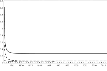
Figure 1: Conditional Mean Squared Errors

This figure reports $\mathsf{tr}(\mathbf{P}_{t|s})$ when using $\widehat{\bm{\Theta}}$, computed for the data analyzed in Section 4, where: $s=t-1$ is the one-step-ahead conditional MSE (solid line); $s=t$ is KF conditional MSE (dashed line); $s=T$ is the KS conditional MSE (dashed-dotted line).

The results in Proposition 1 extend those by Doz et al. (2011, 2012) to the non-stationary case. A major difference between the EM algorithm in levels proposed in this paper, and the EM algorithm in first differences proposed by Doz et al. (2012), is relative to the way idiosyncratic components are modelled. Indeed, while by considering first differences it is implicitly assumed that all idiosyncratic components have a unit root, in our case we can distinguish between stationary and non-stationary idiosyncratic components — i.e., we can allow for idiosyncratic trends only in some variables. This is not a minor difference, as it has substantial implications for the properties of the estimators.

First of all we model non-stationary idiosyncratic components as additional latent states rather than differencing them, thus improving efficiency (see also Remark 2 below). Second, when $\xi_{it}\sim I(0)$, under D1 and D2 the QML estimator of the loadings of the $i$-th variable is obtained by minimizing the sample variance of $\xi_{it}$. In this case this is not the same as differencing before estimation, since in that case the loadings would be estimated by minimizing the sample variance of $\Delta\xi_{it}$. The resulting common component of the $i$-th variable has therefore different empirical properties: compared to our non-stationary approach, the common component estimated in first differences is likely to provide a better fit of the first differenced data, but not necessarily of the levels. Conversely, the common component obtained with our approach is likely to provide a better fit of the levels thus capturing better the lower frequencies — and so the long-run trends — and resulting in a smoother estimator, which however might have a worse fit of the differenced data.

We conclude this section by briefly discussing the possible mis-specifications introduced by assumptions D1, D2 and D3. In particular, we assume the vector of idiosyncratic shocks $\bm{e}_{t}$ to be i.i.d. Gaussian, thus imposing four restrictions on: (1) the cross-sectional dependence; (2) the variances; (3) the serial dependence; (4) the distribution. Let us consider the implications for the properties of the estimators of each of these restrictions — see also Doz et al. (2011) for a similar discussion.

Remark 1.

If the idiosyncratic components have some cross-sectional dependence, as allowed by A5, then the state-space form of the model is mis-specified, however by inspecting the proofs we see that, as long as we use an invertible estimator of $\mathbf{R}$, consistency is not affected as long as $n\to\infty$. As a consequence of this asymptotic argument, we do not attempt here to model the off-diagonal terms of $\mathbf{R}$.

This is better illustrated by a simple example showing the properties of the KF (an analogous argument holds for the KS). Denote as $\mathbf{P}$ the steady state of $\mathbf{P}_{t|t-1}$ then it can be shown that $\mathbf{P}=\mathbf{H}\mathbf{H}^{\prime}$ (Lemma 4). Consider the case in which the parameters are given, $\bm{\xi}_{t}\sim I(0)$, and $r=q$, so that $\mathbf{P}$ is invertible, then for $t\geq\bar{t}(T)$ the KF estimator is such that

$$\mathbf{F}_{t|t} =\mathbf{F}_{t|t-1}+\mathbf{P}\bm{\Lambda}^{\prime}(\bm{\Lambda}\mathbf{P}\bm{\Lambda}^{\prime}+\mathbf{R})^{-1}(\mathbf{x}_{t}-\bm{\Lambda}\mathbf{F}_{t|t-1})$$

$$=\mathbf{F}_{t|t-1}+(\bm{\Lambda}^{\prime}\mathbf{R}^{-1}\bm{\Lambda}+\mathbf{P}^{-1})^{-1}\bm{\Lambda}^{\prime}\mathbf{R}^{-1}(\mathbf{x}_{t}-\bm{\Lambda}\mathbf{F}_{t|t-1})$$

$$=(\bm{\Lambda}^{\prime}\mathbf{R}^{-1}\bm{\Lambda})^{-1}\bm{\Lambda}^{\prime}\mathbf{R}^{-1}\mathbf{x}_{t}+O(n^{-1})$$

$$=\mathbf{F}_{t}+(\bm{\Lambda}^{\prime}\mathbf{R}^{-1}\bm{\Lambda})^{-1}\bm{\Lambda}^{\prime}\mathbf{R}^{-1}\bm{\xi}_{t}+O(n^{-1})$$

$$=\mathbf{F}_{t}+O_{p}(n^{-1/2}),$$

where we used (in order) the Woodbury formula, assumption C2, the definition of $\mathbf{x}_{t}$ in (12), and assumption A5. Clearly consistency of the KF does not depend on the specific assumption for $\mathbf{R}$, as long as it is invertible. However for finite $n$ the KF depends on $\mathbf{R}$ and modeling also its out of diagonal terms could in principle improve its efficiency (e.g. Bai and Liao, 2016).

Remark 2.

From the example in Remark 1 it is clear that for finite $n$ the KF estimator is a weighted average of the data where the heteroskedasticity of the idiosyncratic components is accounted for. Again the same argument holds also for the KS. In this respect the KF-KS approach is analogous to the generalized principal component estimator, which is however derived in a stationary setting and without explicitly addressing the dynamics of the data (Choi, 2012).

Remark 3.

If the idiosyncratic components are autocorrelated, then, unless we model them explicitly as additional latent states, optimality is lost, in particular the loadings’ estimators are still consistent but not efficient. By means of D1 we partially solve the problem at least for the series with $I(1)$ idiosyncratic components.

Remark 4.

If the idiosyncratic components are non-Gaussian then the estimator is not optimal being only the best linear estimator. Nevertheless, it has to be noticed that typical macroeconomic data show little deviations from normality, so we are minimally concerned by the restrictions imposed by this assumption.

Summing up, regardless of these mis-specifications even though we might not have the most efficient estimator, we are likely to have gains in efficiency with respect to those estimators obtained by integrating the principal components of first differences of the data (Bai and Ng, 2004). Indeed, principal components are optimal only in the case of serially and cross-sectionally i.i.d. Gaussian idiosyncratic components (Lawley and Maxwell, 1971; Tipping and Bishop, 1999), and such conditions clearly do not hold in a time series context, especially when non-stationarities are present and the cross-sectional dimension is large. On the contrary, our approach explicitly takes into account the autocorrelation in the factors and in the idiosyncratic components as well as their heteroscedasticity, and, as discussed above, it delivers consistent estimates even when some degree of cross-sectional dependence is present but not modelled.

3.3 Trend and cycles

We now turn to estimation of common trends and common cycles. Notice that since we do not fully impose R1, the dynamic factors $\bm{f}_{t}$ are not identified and instead we have to deal with a TC decomposition of the static factors $\mathbf{F}_{t}$, which can be carried out analogously to the one described in Section 2 for $\bm{f}_{t}$. Because of assumption C1 and restriction R3, for given values of $q$ and $d$, the vector $\mathbf{F}_{t}$ admits the factor representation:

$${\mathbf{F}}_{t} =\bm{\Phi}_{1}\mathbf{T}_{t}+\bm{\Gamma}_{t},$$

where $\bm{\Gamma}_{t}\sim I(0)$, $\bm{\Phi}_{1}$ is $r\times(q-d)$ and $\mathbf{T}_{t}$ is the vector of $(q-d)$ common trends with components $T_{jt}\sim I(1)$ for $j=1,\ldots,(q-d)$. Hence, in general the common trends admit the MA representation:

$$\Delta\mathbf{T}_{t}=\bm{\mathcal{B}}(L)\bm{\eta}_{t},$$

where $\bm{\eta}_{t}\stackrel{{\scriptstyle w.n.}}{{\sim}}(\mathbf{0}_{q-d},\bm{\Sigma}_{\eta})$ with $\bm{\Sigma}_{\eta}$ positive definite and $\bm{\mathcal{B}}(L)$ is a $(q-d)\times(q-d)$ one-sided, infinite matrix polynomial with square-summable coefficients and $\mathsf{rk}(\bm{\mathcal{B}}(1))=(q-d)$.

As a consequence of the results by Peña and Poncela (1997) and Proposition 1 above, given the estimated factors $\widehat{\mathbf{F}}_{t}$, it is clear that, as $n,T\to\infty$,

$$\widehat{\mathbf{S}}:=\frac{1}{T^{2}}\sum_{t=1}^{T}\widehat{\mathbf{F}}_{t}\widehat{\mathbf{F}}_{t}^{\prime}\stackrel{{\scriptstyle}}{{\Rightarrow}}\bm{\Phi}_{1}\,\bm{\mathcal{B}}(1)\,\bm{\Sigma}_{\eta}^{1/2}\left(\int_{0}^{1}\bm{\mathcal{W}}(u)\bm{\mathcal{W}}(u)^{\prime}\mathrm{d}u\right)\bm{\Sigma}_{\eta}^{1/2}\,\bm{\mathcal{B}}(1)^{\prime}\,\bm{\Phi}_{1}^{\prime},$$ (19)

where convergence is in the sense of weak convergence of the associated probability measures and $\{\bm{\mathcal{W}}(u),\ 0\leq u\leq 1\}$ is a $(q-d)$-dimensional standard Wiener process. Hence, by virtue of (19), we can estimate the common trends $\mathbf{T}_{t}$ as the first $(q-d)$ principal components of the estimated static factors $\widehat{\mathbf{F}}_{t}$ (Bai, 2004; Peña and Poncela, 2006). Specifically, we denote by $(\widehat{\bm{\Phi}}_{1}\;\widehat{\bm{\Phi}}_{0})$ the $r\times r$ matrix with columns given by the normalized eigenvectors of $\widehat{\mathbf{S}}$, ordered according to the decreasing value of the corresponding eigenvalues, and such that $\widehat{\bm{\Phi}}_{1}$ is $r\times(q-d)$ and $\widehat{\bm{\Phi}}_{0}$ is $r\times(r-q+d)$. This leads to the estimator of common trends as the projection:

$$\widehat{\mathbf{T}}_{t}=\widehat{\bm{\Phi}}_{1}^{\prime}\widehat{\mathbf{F}}_{t}.$$

As for the common cycles, notice first that, by projecting $\widehat{\mathbf{F}}_{t}$ onto the columns of $\widehat{\bm{\Phi}}_{0}$, we obtain the $(r-q+d)$-dimensional process

$$\widehat{\mathbf{G}}_{t}=\widehat{\bm{\Phi}}_{0}^{\prime}\widehat{\mathbf{F}}_{t},$$

which, by construction, is orthogonal to $\widehat{\mathbf{T}}_{t}$. Moreover, $\widehat{\mathbf{G}}_{t}$ is stationary since it belongs to the cointegration space of $\widehat{\mathbf{F}}_{t}$ (Zhang et al., 2016). However, by R3 we know that the cointegration space must have dimension $d$, but we do not impose R3 when estimating the static factors. Thus, we face the problem of identifying $d$ cycles from the higher-dimensional stationary process $\widehat{\mathbf{G}}_{t}$.

In order to identify the common cycles we then look for the $d$-dimensional projection of $\widehat{\mathbf{G}}_{t}$ with maximum spectral density. In the empirical analysis of Section 4, we consider the VAR(2):

$$\widehat{\mathbf{G}}_{t}=\bm{\mathcal{A}}_{1}\widehat{\mathbf{G}}_{t-1}+\bm{\mathcal{A}}_{2}\widehat{\mathbf{G}}_{t-2}+\bm{v}_{t},$$ (20)

where $\bm{v}_{t}\stackrel{{\scriptstyle w.n.}}{{\sim}}(\mathbf{0}_{r-q+d},\bm{\Sigma}_{v})$ and $\det(\mathbf{I}_{r-q+d}-\bm{\mathcal{A}}_{1}z-\bm{\mathcal{A}}_{2}z^{2})\neq 0$ for $|z|\leq 1$. Once we estimate (20) we have its residuals $\widehat{\bm{v}}_{t}$ and their covariance matrix $\widehat{\bm{\Sigma}}_{v}$. Denote as $\widehat{\bm{\mathcal{H}}}$ the $(r-q+d)\times d$ matrix having as columns the leading $d$ normalized eigenvectors of $\widehat{\bm{\Sigma}}_{v}$. We then define the estimated cycle component as the $d$-dimensional projection:

$$\widehat{\mathbf{C}}_{t}=\widehat{\bm{\mathcal{H}}}^{\prime}\widehat{\mathbf{G}}_{t}.$$

The estimated TC decomposition is then given by

$$\widehat{\mathbf{F}}_{t} =\widehat{\bm{\Phi}}_{1}\widehat{\bm{\Phi}}_{1}^{\prime}\widehat{\mathbf{F}}_{t}+\widehat{\bm{\Phi}}_{0}\widehat{\bm{\Phi}}_{0}^{\prime}\widehat{\mathbf{F}}_{t}$$

$$=\widehat{\bm{\Phi}}_{1}\widehat{\mathbf{T}}_{t}+\widehat{\bm{\Phi}}_{0}\widehat{\mathbf{G}}_{t}$$

$$=\widehat{\bm{\Phi}}_{1}\widehat{\mathbf{T}}_{t}+\widehat{\bm{\Phi}}_{0}\widehat{\bm{\mathcal{H}}}\widehat{\bm{\mathcal{H}}}^{\prime}\widehat{\mathbf{G}}_{t}+\widehat{\bm{\Phi}}_{0}\widehat{\bm{\mathcal{H}}}_{\perp}\widehat{\bm{\mathcal{H}}}^{\prime}_{\perp}\widehat{\mathbf{G}}_{t}$$

$$=\widehat{\bm{\Phi}}_{1}\widehat{\mathbf{T}}_{t}+\widehat{\bm{\Phi}}_{0}\widehat{\bm{\mathcal{H}}}\widehat{\mathbf{C}}_{t}+\widehat{\bm{\Phi}}_{0}(\widehat{\mathbf{G}}_{t}-\widehat{\bm{\mathcal{H}}}\widehat{\mathbf{C}}_{t}),$$ (21)

where $\widehat{\bm{\mathcal{H}}}_{\perp}$ is $(r-q+d)\times(r-q)$ and such that $\widehat{\bm{\mathcal{H}}}_{\perp}^{\prime}\widehat{\bm{\mathcal{H}}}=\mathbf{0}_{(r-q)\times d}$. The last term on the right-hand-side of (21) appears due to the mis-specification caused by not fully imposing R1 and R3 and in particular it has covariance of rank $(r-q)$ and since $r>q$ it is in general not zero.

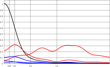
Figure 2: Spectral Densities of Common Trends and Common Cycles

This figure reports for the data analyzed in Section 4 the spectral densities of the common trend $\Delta\widehat{\mathbf{T}}_{t}$ (black line), the common cycles $\Delta\widehat{\mathbf{C}}_{t}$ (red lines), and the residual cycles $(\Delta\widehat{\mathbf{G}}_{t}-\widehat{\bm{\mathcal{H}}}\Delta\widehat{\mathbf{C}}_{t})$ (blue lines). On the horizontal axis we report periods $\tau_{j}$ measured in years and corresponding to frequencies $\omega_{j}=\frac{2\pi}{4\tau_{j}}$ (the data considered is quarterly).

To appreciate the meaning and the appropriateness of decomposition (21), in Figure 2 we show the spectral densities of the first differences of the three components of $\widehat{\mathbf{F}}_{t}$ for the data analyzed in Section 4, where $r=6$, $q=3$, and $d=2$. As expected the estimated common trend $\widehat{\mathbf{T}}_{t}$ (black line) contributes most at the lowest frequencies — i.e., lower than $\frac{\pi}{10}$ — which correspond to periods higher than five years. Once we remove the common trend, of the remaining five processes $\widehat{\mathbf{G}}_{t}$, the two estimated common cycles $\widehat{\mathbf{C}}_{t}$ (red lines) capture most of the variation for almost all frequencies: one cycle dominates at periods longer than two years — i.e., frequencies lower than $\frac{\pi}{4}$ — and the other cycle dominates at periods shorter than two years — i.e., frequencies higher than $\frac{\pi}{4}$. With respect to those two cycles, the residual three cycles $(\widehat{\mathbf{G}}_{t}-\widehat{\bm{\mathcal{H}}}\widehat{\mathbf{C}}_{t})$ (blue lines) give a negligible contributions to the total variation. Given this empirical result, the extra term in (21) can be neglected and treated as a mis-specification error.

Finally, from (21), the estimated TC decomposition of the data immediately follows:

$$x_{it} =\widehat{\bm{\lambda}}_{i}^{\prime}\widehat{\bm{\Phi}}_{1}\widehat{\mathbf{T}}_{t}+\widehat{\bm{\lambda}}_{i}^{\prime}\widehat{\bm{\Phi}}_{0}\widehat{\bm{\mathcal{H}}}\widehat{\mathbf{C}}_{t}+\widehat{\bm{\lambda}}_{i}^{\prime}\widehat{\bm{\Phi}}_{0}(\widehat{\mathbf{G}}_{t}-\widehat{\bm{\mathcal{H}}}\widehat{\mathbf{C}}_{t})+\widehat{\xi}_{it},$$

which is the estimated counterpart of the representation given in (9).

4 Estimating the cyclical position of the economy
and the observation error

We now use our model to estimate the cyclical position of the US economy and the observation error. In particular, in Section 4.1 we will estimate “the observation error” by estimating the non-stationary approximate DFM as explained in Section 3.2. And, in Section 4.2 we will estimate “the cyclical position of the economy” by decomposing the common factors into common trends and common cycles using the TC decomposition discussed in Sections 2 and 3.3.

The following analysis is carried out on a large macroeconomic dataset comprising $n=103$ quarterly series from 1960:Q1 to 2017:Q1 describing the US economy. The complete list of variables and transformations is reported in Appendix D.

Compared to the papers that use small DFMs to estimate the cyclical position of the economy, which typically estimate the output gap using only high level variables such as GDP, the unemployment rate, and PCE price inflation, we include several other indicators, thus being able to capture information coming from a wider spectrum of the economy. Specifically, our datasets includes national account statistics, industrial production indexes, various price indexes including CPIs, PPIs, and PCE price indexes, various labor market indicators including indicators from both the household survey and the establishment survey as well as labor cost and compensation indexes, monetary aggregates, credit and loans indicators, housing market indicators, interest rates, the oil price, and the S&P500 index. Broadly speaking, all the variables that are $I(1)$ are not transformed, while all the variables that are $I(2)$ are differenced once. Notice that some variables should from a theoretical economic point of view always be considered as $I(0)$ (e.g. inflation rates, unemployment rate, and interest rates) but since they exhibit a great deal of persistence are here treated as $I(1)$. Finally, a linear trend is estimated where necessary before applying our methodology, thus accounting for the deterministic component in (1).

A thorough empirical analysis requires tackling two main preliminary problems. First, we need to determine the number of common trends $(q-d)$, of common shocks $q$, and of static factors $r$. To determine the number of common trends $(q-d)$ we use the criterion by Barigozzi et al. (2016b), which exploits the behaviour of the eigenvalues described in condition B2. This criterion indicates the presence of $(q-d)=1$ common trend, which is in line with many theoretical models assuming a common productivity trend as the sole driver of long-run dynamics (e.g. Del Negro et al., 2007). To determine the number of common shocks $q$ we use the test by Onatski (2009) and the criterion by Hallin and Liška (2007), which exploit the behaviour of the eigenvalues described in condition B1. Both methods indicate the presence of $q=3$ common shocks. Having determined $q$, as we explained in Section 3.1 by virtue of R2 we can set the number of static factors $r$ according to their explained variance. By looking at Table 1 we can clearly see that $r\simeq 2q$, and therefore in our benchmark specification we set $q=3$ and $r=6$.

Table 1: Percentage of explained variance

	1	2	3	4	5	6	7	8	9	10
$q$	33.4	45.8	53.3	58.9	63.6	67.4	70.6	73.4	75.8	77.9
$r$	23.4	33.9	42.1	47.9	51.8	55.3	58.2	60.6	62.7	64.9

This table reports the percentage of total variance explained by the $q$ largest eigenvalues of the spectral density matrix of $\Delta\mathbf{x}_{t}$ and by the $r$ largest eigenvalues of the covariance matrix of $\Delta\mathbf{x}_{t}$.

Second, we need to choose which idiosyncratic components to model as random walk, and which as white noises. Following the methodology proposed by Bai and Ng (2004), we can explicitly test the null-hypothesis $H_{0}$: ${\rho}_{i}=1$, and if we do not reject $H_{0}$, we set $\rho_{i}=1$, while if we reject $H_{0}$, we set $\rho_{i}=0$. This approach is applied to all variables in the dataset except GDP, GDI, unemployment rate, Federal funds rate, and CPI, core CPI, PCE, and core PCE inflation, for which we impose a priori $\rho_{i}=0$. That is, while for most of the variables in the dataset we let the data determine what is driving their long run dynamics, we impose that the long-run dynamics of GDP, GDI, unemployment rate, Federal funds rate, and CPI, core CPI, PCE, and core PCE inflation are driven exclusively by macroeconomic shocks, with the idiosyncratic shocks accounting only for short-run movement.

4.1 Measuring Gross Domestic Output

A fundamental issue in economics is the measurement of aggregate real output, henceforth Gross Domestic Output (GDO). Historically, GDO has been measured mainly by the Gross Domestic Product (GDP), but GDP, which tracks all expenditures on final goods and services produced, is just an estimate of GDO. An equally acceptable estimate of the concept of GDO is represented by the Gross Domestic Income (GDI), which tracks all income received by those who produced the output. GDP is almost always preferred to GDI, the main reason being that it is released before GDI. However it has been shown that GDI reflects the business cycle fluctuations in true output growth better than GDP and moreover GDI is better than GDP in recognising the start of a recession (Nalewaik, 2010, 2012).

In recent years, there has been interest in combining GDP and GDI to come up with a better estimate of GDO, where the rationale for doing so is that the difference between GDP and GDI is exclusively the result of measurement error — using the NIPA table definition “statistical discrepancy” — as these two statistics are in fact measuring the same thing. For example, starting from November 4, 2013, the Philadelphia Fed releases an estimate of GDO, called “GDPplus” proposed by Aruoba et al. (2016), which is defined as the common component of a bivariate one-factor model built with GDP and GDI growth rates. Similarly, and starting from July 30, 2015, the Bureau of Economic Analysis (BEA) releases “the average of GDP and GDI”, which the Council of Economic Advisers refers to as GDO (Council of Economic Advisers, 2015).

Our approach differs from those mentioned above in that our estimate of GDO is not obtained by combining GDP and GDI, rather it is obtained by using all the 103 variables included in our dataset. In detail, we define GDO as that part of GDP/GDI that is driven by the macroeconomic (common) shocks, i.e., $\textrm{GDO}_{t}=\chi_{t}^{\textrm{GDP}}=\chi_{t}^{\textrm{GDI}}$. To estimate GDO in this way, we estimate a constrained version of model (12)-(13), where we impose the restriction of equal common components: $\chi_{t}^{\textrm{GDP}}=\chi_{t}^{\textrm{GDI}}$. This restriction is indeed corroborated by the data, as even if we do not impose it, the estimated $\chi_{t}^{\textrm{GDP}}$ and $\chi_{t}^{\textrm{GDI}}$ are nearly identical. In numbers, the standard deviation of $(\Delta y_{t}^{\textrm{GDP}}-\Delta y_{t}^{\textrm{GDI}})$ is 1.93, while the standard deviation of $(\Delta\chi_{t}^{\textrm{GDP}}-\Delta\chi_{t}^{\textrm{GDI}})$ is reduced to 0.28.

Figure 3: Gross Domestic Output

Quarterly annualised percentage change	4-quarter percentage change

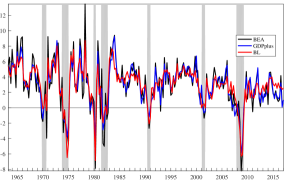
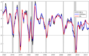
This figure reports different estimates of GDO. Black line: “the average of GDP and GDI” released by the BEA; blue line: “GDPplus” released by the Philadelphia Fed; red line: our estimate.

Figure 3 shows our proposed estimate of GDO (red line) together with “GDPplus” (blue line) and the “the average of GDP and GDI” released by the BEA (black line). Overall, the three measures are very similar, which is not surprising, as they are attempting to estimate the same quantity. However, three important differences emerges.

First, our estimate of GDO is smoother than the other two. This is not surprising. Compared to “GDPplus” and “the average of GDP and GDI”, our estimate of GDO is constructed to contain a larger low frequency component, because it is estimated on data in levels rather than on growth rates. Moreover, because it is derived under the assumption that the idiosyncratic components of GDP and GDI are stationary, by construction our estimate of GDO captures all the low frequency movements of GDP and GDI.

Second, our estimate of GDO does not show any kind of residual seasonality in the last fifteen years, where the term “residual seasonality” refers to the presence of “lingering seasonal effects even after seasonal adjustment processes have been applied to the data” (Moulton and Cowan, 2016). Mainly motivated by the fact that since 2010 GDP growth in Q1 has been on average more than 1 percentage point lower than in the other quarters (NW plot of Figure 4), in recent years there has been lots of discussion on whether US GDP exhibit residual seasonality or not. The profession is not in agreement on this issue, as some authors (e.g. ; , ) conclude that US GDP does not exhibit residual seasonality, while others (e.g. Rudebusch et al., 2015; Lunsford, 2017) find evidence of residual seasonality — see Moulton and Cowan (2016) for a technical discussion on causes and remedies for residual seasonality in US GDP. Figure 4 shows average real GDO growth by quarter for our estimate of GDO (SE plot), “GDPplus” (SW plot), and “the average of GDP and GDI” (NE plot). As can be clearly seen, our estimate of GDO exhibits no residual seasonality whatsoever in the last 15 years.

Figure 4: Residual Seasonality

GDP	BEA
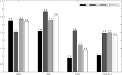
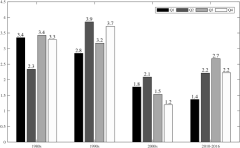
GDPplus	BL

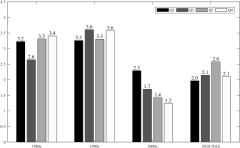
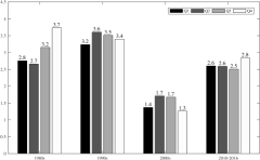
This figure reports average growth at an annual rate by quarter for GDP, “the average of GDP and GDI” released by the BEA, the Philadelphia Fed estimate of GDO (GDPplus), and our estimate of GDO (BL).

Third, our estimate of GDO in the recent years gives a different signal about the economy than the one given by ‘GDPplus” and “the average of GDP and GDI”. According to our estimate, since 2010 quarterly annualized GDO growth was on average $\nicefrac{{1}}{{2}}$ of a percentage point higher than estimated by the BEA or the Philadelphia Fed, where this difference comes mainly from our estimate of GDO growth in the first quarter (see Figure 4), and therefore from the fact that our measure do not suffer of residual seasonality. In other words, based on the commonality in the data, the US economy grew at a faster pace than measured by national account statistics.

4.2 Measuring the output gap

Decomposing aggregate real output into potential output and output gap is a critical task for both monetary and fiscal policy, as the former is a key input for long-term projections, and the latter can be an important gauge of inflationary pressure. There exist many definitions of potential output and of output gap — see Kiley, 2013, for a survey of different methods and definitions. Here we use the definition implied by the TC decomposition discussed in Sections 2 and 3.3. Among the many existing approaches the most similar to ours are Fleischman and Roberts (2011) and Jarociński and Lenza (2016), who use small dynamic factor models, Aastveit and Trovik (2014), who use a large stationary dynamic factor model combined with the Hodrick Prescott filter, and Morley and Wong (2017), who use a large stationary BVAR combined with the Beveridge and Nelson decomposition.

We compare our output gap estimate with the one produced by the Congressional Budget Office (CBO). The CBO estimates potential output and the output gap by using the so-called “production function approach” according to which potential output is that level of output consistent with current technologies and normal utilisation of capital and labour, and the output gap is the residual part of output. Specifically, the CBO model is based upon a textbook Solow growth model, with a neoclassical production function. Labour and productivity trends are estimated by using a variant of the Okun’s law, so that actual output is above its potential (the output gap is positive), when the unemployment rate is below the natural rate of unemployment, which is in turn defined as the non-accelerating inflation rate of unemployment (NAIRU), i.e., that level of unemployment consistent with a stable inflation — for further details see Congressional Budget Office (2001).

In Figure 5, we compare our measure of the output gap (red line) with the one produced by the CBO (blue line), where the left plot shows the level of the output gap, while the right plot shows the 4-quarter percentage change of the output gap. The main result emerging from Figure 5 is that our estimate of the output gap is remarkably similar to that of the CBO. However, there are a few periods in which the two estimates diverge, among which the main one is from the late nineties to the financial crisis. In particular, while according to the CBO the level of the output gap was negative between 2001:Q1 and 2005:Q4, according to our estimate in that same period the output gap was positive — on average 2$\nicefrac{{1}}{{2}}$ percentage points higher than estimated by the CBO. Therefore, according to our estimate the level of the output gap right before the great financial crisis in 2007:Q4 was 1.3%, while according to the CBO was -0.7%, and hence we estimate that the level of slack in the economy at the trough of the crisis in 2009:Q2 was -4.5%, approximately 1$\nicefrac{{3}}{{4}}$ percentage points higher than estimated by the CBO.

Figure 5: Output gap

Level	4-quarter percentage change

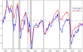
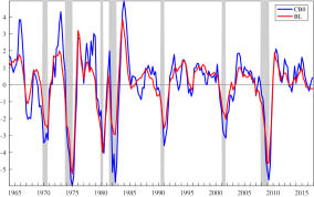
The left plot shows the level of the output gap estimated by the CBO (blue line) together with our estimate (red line). The right plot shows the 4-quarter percentage change of the output gap.

To conclude, let us emphasize that the fact that our estimate of the output gap is close to that of the CBO is a remarkable result, particularly so because our estimate of the output gap is very different from that of the CBO from both a technical and an interpretational point of view. Indeed, while the CBO constructs the output gap so that its level has a specific economic meaning, our measure of the output gap is simply the transitory/stationary part of the common component of output — i.e., that part of aggregate real output that will disappear in the long-run. Therefore, our output gap estimate provides different and complementary information on the cyclical position of the economy than that contained in the CBO estimate. In particular, our estimate of the output gap seems more suitable to answer the question “which part of current growth is due to temporary factors?”, while the measure of the CBO is certainly more suitable as a gauge of inflation pressure. This can explain in part the divergence of the two estimates in the 2000s. This period is characterized by stable and low inflation — on average core CPI inflation between 2001:Q1 and 2007:Q4 was approximately 2.1%. Accordingly, the CBO estimates that slack is positive (i.e., the output gap negative). By contrast, our measure, which is not specifically affected by inflation, but it is more broadly influenced by the co-movement in the data, estimates that a part of the aggregate real output was transitory. This makes sense given that the years before the crisis were characterized by several factors that proved indeed transitory, such as the housing boom, a historically high share of sub-prime loan origination (Haughwout and Okah, 2009), and a large amount of equity withdrawal from housing (Fuster et al., 2017). And, since our model includes a large number of variables, including housing indicators as well as loan and credit indicators, these transitory factors are captured by our model.

5 Discussion and conclusions

In this paper we disentangle long-run co-movements (common trends) from short-run co-movements (common cycles) in large datasets. To this end, we first estimate a non-stationary dynamic factor model by means of a Quasi Maximum Likelihood estimator based on the Expectation Maximisation algorithm, combined with the Kalman Filter and the Kalman Smoother estimators of the factors. We then disentangle common trends from common cycles by applying a non-parametric Trend-Cycle decomposition to the latent common factors and based on eigenanalysis of their long-run covariance. The asymptotic properties of this estimator are derived and discussed in the paper.

We estimate our model on a large panel of US quarterly macroeconomic time series with the goal of estimating the cyclical position of the economy and the observation error. After backing out the observation error, we show that our model naturally produces an estimate of aggregate real output, which we refer to as Gross Domestic Output (GDO). According to our estimate of GDO, since 2010 the US economy grew at a faster pace than measured by national account statistics.

We then use a Trend-Cycle decomposition to estimate the output gap. We compare our estimate of the output gap, which is entirely data-driven, with that produced by the Congressional Budget Office (CBO), which is instead based on theoretical economic models. It turns out that our estimate of the output gap is remarkably similar to that of the CBO except from the late nineties to the financial crisis, when our measure suggests that a greater part of the produced output was driven by transitory factors.

There are a number of aspects of our model that we have not fully developed in our empirical analysis and that are left for future research. First, due to the use of the Kalman Filter, our factor estimator is in principle able to handle both mixed frequency and missing data (e.g. Mariano and Murasawa, 2003; Jungbacker et al., 2011; Bańbura and Modugno, 2014) and, therefore, it can be used for real-time analysis (Giannone et al., 2008). This aspect is well-known to be particularly relevant when estimating the output gap, since as shown by Orphanides and van Norden (2002), end-of-sample revisions of GDP are of the same order of magnitude as the gap itself. Second, the use of the Kalman Filter makes our model suitable for scenario and counterfactual analysis based on conditional forecasts (Bańbura et al., 2015). Third, as shown in equation (21), our model naturally produces a Trend-Cycle decomposition for each variable in the dataset, and therefore it is possible to estimate other policy-relevant indicators, such as the unemployment gap (in our framework, the cycle component of the unemployment rate) or trend inflation (in our framework, the trend component of core CPI or the core PCE price indexes).

Our approach has been so far deliberately entirely data driven, and we have been careful in imposing the least possible amount of restrictions to let the data speak freely. This approach has undeniably some important merits, as estimation of GDO seems to fit naturally in our framework, and the Trend-Cycle decomposition that we obtain for GDO is economically sensible. However, we believe that imposing the statistical restrictions described in Section 3.1, thus eliminating the miss-specification error when computing the Trend-Cycle decomposition, as well as imposing economically meaningful constraints, seems to be an essential step forward. Our view is that one way to proceed is to consider Bayesian estimation of the model, so that our economic and statistical knowledge of the data can be included by means of suitable priors. All this is the subject of our current research.

Appendix A Representation results

Hereafter, and throughout all appendices, we consider restriction R2 when $s=1$ as found empirically in Section 4. Therefore, $r=2q$.

A.1 Proof of restriction R3

For the dynamic factors consider the VECM(2)

$$\Delta\bm{f}_{t}=-\mathbf{a}\mathbf{b}^{\prime}\bm{f}_{t-3}+\bm{\Gamma}_{1}\Delta\bm{f}_{t-1}+\bm{\Gamma}_{2}\Delta\bm{f}_{t-2}+\mathbf{u}_{t},$$ (A1)

where $\mathbf{a}$ and $\mathbf{b}$ are $q\times d$ and for simplicity we consider just the case of two lags since this will imply a VECM(1) and therefore a VAR(2) for the static factors as implemented in (13).

First assume that in R1 we have $\mathbf{K}=\mathbf{I}_{r}$. Our aim is then to find the correct VECM representation for $\mathbf{F}_{t}=(\bm{f}_{t}^{\prime}\;\bm{f}_{t-1}^{\prime})^{\prime}$ when the VECM in (A1), and restrictions R1 and R2 hold. Since we model $\mathbf{F}_{t}$ as a VAR(2) we know that we must have a VECM(1) with reduced rank innovations by R1, hence

$$\Delta\mathbf{F}_{t}=-\bm{\alpha}\bm{\beta}^{\prime}\mathbf{F}_{t}+\mathbf{M}\Delta\mathbf{F}_{t-1}+\mathbf{H}\mathbf{u}_{t},$$ (A2)

where $\bm{\alpha}$ and $\bm{\beta}$ are $r\times c$ with $c<r$ and $\mathbf{H}$ is $r\times q$. Moreover, from Barigozzi et al. (2016a) we have $d\leq c\leq(r-q+d)$. We are then interested in finding $c$, and the expressions of $\mathbf{M}$, $\bm{\alpha}$, $\bm{\beta}$, and $\mathbf{H}$ as functions of the parameters $\mathbf{a}$, $\mathbf{b}$, $\bm{\Gamma}_{1}$, and $\bm{\Gamma}_{2}$ in (A1). Let us write $\bm{\alpha}=(\bm{\alpha}_{1}^{\prime}\;\bm{\alpha}_{2}^{\prime})^{\prime}$ and $\bm{\beta}=(\bm{\beta}_{1}^{\prime}\;\bm{\beta}_{2}^{\prime})^{\prime}$ where $\bm{\alpha}_{1}$, $\bm{\alpha}_{2}$, $\bm{\beta}_{1}$, $\bm{\beta}_{2}$ are all $q\times c$. We also denote as $\mathbf{M}_{ij}$ for $i,j=1,2$ the four $q\times q$ blocks of $\mathbf{M}$ and as $\mathbf{H}_{1}$ and $\mathbf{H}_{2}$ the two $q\times q$ blocks of $\mathbf{H}$. Following Proietti (1997), we define the $(2r+c)$-dimensional vector

$$\mathbf{G}_{t}=\left(\begin{array}[]{l}\Delta\mathbf{F}_{t}\\ \Delta\mathbf{F}_{t-1}\\ \bm{\beta}^{\prime}\mathbf{F}_{t-2}\end{array}\right)=\left(\begin{array}[]{l}\Delta\bm{f}_{t}\\ \Delta\bm{f}_{t-1}\\ \Delta\bm{f}_{t-1}\\ \Delta\bm{f}_{t-2}\\ \bm{\beta}_{1}^{\prime}\bm{f}_{t-2}+\bm{\beta}_{2}^{\prime}\bm{f}_{t-3}\end{array}\right).$$

Then, the state-space form of (A2) is given by

$$\Delta\mathbf{F}_{t} ={\mathbf{Z}}\mathbf{G}_{t},$$

$$\mathbf{G}_{t} ={\mathbf{T}}\mathbf{G}_{t-1}+{\mathbf{Z}}^{\prime}\mathbf{H}\mathbf{u}_{t},$$ (A3)

with the $r\times(2r+c)$ matrix ${\mathbf{Z}}=(\mathbf{I}_{r}\;\mathbf{0}_{r}\;\mathbf{0}_{r\times c})$. Then,

$${\mathbf{Z}}^{\prime}\mathbf{H}=\left(\begin{array}[]{l}\mathbf{I}_{r}\\ \mathbf{0}_{r}\\ \mathbf{0}_{c\times r}\end{array}\right)\left(\begin{array}[]{l}\mathbf{H}_{1}\\ \mathbf{H}_{2}\end{array}\right)=\left(\begin{array}[]{l}\mathbf{H}_{1}\\ \mathbf{H}_{2}\\ \mathbf{0}_{q}\\ \mathbf{0}_{q}\\ \mathbf{0}_{c\times q}\end{array}\right).$$

and the $(2r+c)\times(2r+c)$ matrix ${\mathbf{T}}$ is given by

$${\mathbf{T}}=\left(\begin{array}[]{lll}\mathbf{M}&-\bm{\alpha}\bm{\beta}^{\prime}&-\bm{\alpha}\\ \mathbf{I}_{r}&\mathbf{0}_{r}&\mathbf{0}_{r\times c}\\ \mathbf{0}_{c\times r}&\bm{\beta}^{\prime}&\mathbf{I}_{c}\end{array}\right)=\left(\begin{array}[]{ll | ll | l}\mathbf{M}_{11}&\mathbf{M}_{12}&-\bm{\alpha}_{1}\bm{\beta}_{1}^{\prime}&-\bm{\alpha}_{1}\bm{\beta}_{2}^{\prime}&-\bm{\alpha}_{1}\\ \mathbf{M}_{21}&\mathbf{M}_{22}&-\bm{\alpha}_{2}\bm{\beta}_{1}^{\prime}&-\bm{\alpha}_{2}\bm{\beta}_{2}^{\prime}&-\bm{\alpha}_{2}\\ \hline\cr\mathbf{I}_{q}&\mathbf{0}_{q}&\mathbf{0}_{q}&\mathbf{0}_{q}&\mathbf{0}_{q\times c}\\ \mathbf{0}_{q}&\mathbf{I}_{q}&\mathbf{0}_{q}&\mathbf{0}_{q}&\mathbf{0}_{q\times c}\\ \hline\cr\mathbf{0}_{c\times q}&\mathbf{0}_{c\times q}&\bm{\beta}_{1}^{\prime}&\bm{\beta}_{2}^{\prime}&\mathbf{I}_{c}\\ \end{array}\right).$$

Now using these definitions into (A3) we have five $q$-dimensional equations. The first one is

$$\Delta\bm{f}_{t} =\mathbf{M}_{11}\Delta\bm{f}_{t-1}+\mathbf{M}_{12}\Delta\bm{f}_{t-2}-\bm{\alpha}_{1}\bm{\beta}_{1}^{\prime}\bm{f}_{t-2}-\bm{\alpha}_{1}\bm{\beta}_{2}^{\prime}\bm{f}_{t-3}+\mathbf{H}_{1}\mathbf{u}_{t},$$

which is equivalent to (A1) when

$$\mathbf{M}_{11}=\bm{\Gamma}_{1},\quad\mathbf{M}_{12}=\bm{\Gamma}_{2},\quad\bm{\alpha}_{1}=\mathbf{a},\quad\bm{\beta}_{1}=\mathbf{0}_{q\times c},\quad\bm{\beta}_{2}=\mathbf{b},\quad\mathbf{H}_{1}=\mathbf{I}_{q},\quad c=d.$$ (A4)

The second equation is

$$\Delta\bm{f}_{t-1} =\mathbf{M}_{21}\Delta\bm{f}_{t-1}+\mathbf{M}_{22}\Delta\bm{f}_{t-2}-\bm{\alpha}_{2}\bm{\beta}_{1}^{\prime}\Delta\bm{f}_{t-2}-\bm{\alpha}_{2}\bm{\beta}_{2}^{\prime}\Delta\bm{f}_{t-3}-\bm{\alpha}_{2}\bm{\beta}_{1}^{\prime}\bm{f}_{t-3}-\bm{\alpha}_{2}\bm{\beta}_{2}^{\prime}\bm{f}_{t-4}+\mathbf{H}_{2}\mathbf{u}_{t},$$

from which we see that we must also have

$$\mathbf{M}_{21}=\mathbf{I}_{q},\qquad\mathbf{M}_{22}=\mathbf{0}_{q},\qquad\bm{\alpha}_{2}=\mathbf{0}_{q\times c},\qquad\mathbf{H}_{2}=\mathbf{0}_{q}.$$ (A5)

Under (A4) and (A5) the third, fourth and fifth equation in (A3) are just identities.

By imposing these restrictions we have the mapping between the VECM(1) for $\mathbf{F}_{t}$ in (A2) and the VECM(2) for $\bm{f}_{t}$ in (A1)

$$\mathbf{M}=\left(\begin{array}[]{ll}\bm{\Gamma}_{1}&\bm{\Gamma}_{2}\\ \mathbf{I}_{q}&\mathbf{0}_{q}\end{array}\right),\qquad\bm{\alpha}=\left(\begin{array}[]{l}\mathbf{a}\\ \mathbf{0}_{q\times d}\end{array}\right),\qquad\bm{\beta}=\left(\begin{array}[]{l}\mathbf{0}_{q\times d}\\ \mathbf{b}\end{array}\right),\qquad\mathbf{H}=\left(\begin{array}[]{c}\mathbf{I}_{q}\\ \mathbf{0}_{q}\end{array}\right).$$ (A6)

If we now consider a generic $\mathbf{K}$ in R1, then (A2) holds for $\mathbf{F}_{t}=\mathbf{K}(\bm{f}_{t}^{\prime}\;\bm{f}_{t-1}^{\prime})^{\prime}$ and (A6) becomes

$$\mathbf{M}=\mathbf{K}\left(\begin{array}[]{ll}\bm{\Gamma}_{1}&\bm{\Gamma}_{2}\\ \mathbf{I}_{q}&\mathbf{0}_{q}\end{array}\right)\mathbf{K}^{-1},\qquad\bm{\alpha}=\mathbf{K}\left(\begin{array}[]{l}\mathbf{a}\\ \mathbf{0}_{q\times d}\end{array}\right),\qquad\bm{\beta}={\mathbf{K}^{-1}}^{\prime}\left(\begin{array}[]{l}\mathbf{0}_{q\times d}\\ \mathbf{b}\end{array}\right),\qquad\mathbf{H}=\mathbf{K}\left(\begin{array}[]{c}\mathbf{I}_{q}\\ \mathbf{0}_{q}\end{array}\right).$$

The cointegration rank $c$ of $\mathbf{F}_{t}$ is given by $\mathsf{rk}(\bm{\alpha}\bm{\beta}^{\prime})=d$.

A.2 Reduced and structural form of the state-space representation

Consider (12)-(13) written in matrix notation and using the companion form of the VAR

$$\mathbf{x}_{t} =\bm{\Lambda}\mathbf{F}_{t}+\bm{\xi}_{t},$$ (A7)

$$\left(\begin{array}[]{l}\mathbf{F}_{t}\\ \mathbf{F}_{t-1}\end{array}\right) =\left(\begin{array}[]{cc}\mathbf{A}_{1}&\mathbf{A}_{2}\\ \mathbf{I}_{r}&\mathbf{0}_{r}\end{array}\right)\left(\begin{array}[]{c}\mathbf{F}_{t-1}\\ \mathbf{F}_{t-2}\end{array}\right)+\left(\begin{array}[]{c}\mathbf{H}\\ \mathbf{0}_{r\times q}\end{array}\right)\mathbf{u}_{t},$$ (A16)

with $\bm{\Lambda}=(\bm{\lambda}_{1}\cdots\bm{\lambda}_{n})^{\prime}$ the $n\times r$ loadings matrix. We call (A7)-(A16) the reduced form of the model. Similarly consider the structural form, where, for convenience, in the VAR we write twice the same equation:

$$\mathbf{x}_{t} =\mathbf{B}_{0}\bm{f}_{t}+\mathbf{B}_{1}\bm{f}_{t-1}+\bm{\xi}_{t},$$ (A17)

$$\left(\begin{array}[]{c}\bm{f}_{t}\\ \bm{f}_{t-1}\\ \bm{f}_{t-1}\\ \bm{f}_{t-2}\end{array}\right) =\left(\begin{array}[]{cccc}\bm{\Pi}_{1}&\bm{\Pi}_{2}&\mathbf{0}_{q}&\bm{\Pi}_{3}\\ \mathbf{I}_{q}&\mathbf{0}_{q}&\mathbf{0}_{q}&\mathbf{0}_{q}\\ \mathbf{I}_{q}&\mathbf{0}_{q}&\mathbf{0}_{q}&\mathbf{0}_{q}\\ \mathbf{0}_{q}&\mathbf{I}_{q}&\mathbf{0}_{q}&\mathbf{0}_{q}\\ \end{array}\right)\left(\begin{array}[]{c}\bm{f}_{t-1}\\ \bm{f}_{t-2}\\ \bm{f}_{t-2}\\ \bm{f}_{t-3}\end{array}\right)+\left(\begin{array}[]{c}\mathbf{I}_{q}\\ \mathbf{0}_{q}\\ \mathbf{0}_{q}\\ \mathbf{0}_{q}\end{array}\right)\mathbf{u}_{t},$$ (A34)

where $\mathbf{B}_{0}=(\bm{b}_{01}\cdots\bm{b}_{0n})^{\prime}$, $\mathbf{B}_{1}=(\bm{b}_{11}\cdots\bm{b}_{1n})$ are both $n\times q$. Because of R1 there exists an invertible $r\times r$ matrix $\mathbf{K}$ such that

$$\mathbf{F}_{t}=\mathbf{K}(\bm{f}_{t}^{\prime}\,\bm{f}_{t-1}^{\prime})^{\prime}, \qquad(\bm{f}_{t}^{\prime}\,\bm{f}_{t-1}^{\prime})^{\prime}=\mathbf{K}^{-1}\mathbf{F}_{t},$$ (A35)

$$\bm{\Lambda}=(\mathbf{B}_{0}\,\mathbf{B}_{1})\mathbf{K}^{-1}, \qquad(\mathbf{B}_{0}\,\mathbf{B}_{1})=\bm{\Lambda}\mathbf{K}.$$ (A36)

By comparing (A7)-(A16) with (A17)-(A34) and using (A35)-(A36), we have the parameters of the reduced form

$$\mathbf{A}_{1}=\mathbf{K}\left(\begin{array}[]{cc}\bm{\Pi}_{1}&\bm{\Pi}_{2}\\ \mathbf{I}_{q}&\mathbf{0}_{q}\end{array}\right)\mathbf{K}^{-1},\qquad\mathbf{A}_{2}=\mathbf{K}\left(\begin{array}[]{cc}\mathbf{0}_{q}&\bm{\Pi}_{3}\\ \mathbf{0}_{q}&\mathbf{0}_{q}\end{array}\right)\mathbf{K}^{-1},\qquad\mathbf{H} =\mathbf{K}\left(\begin{array}[]{c}\mathbf{I}_{q}\\ \mathbf{0}_{q}\end{array}\right).$$ (A43)

The relations (A35), (A36) and (A43) are used throughout the following. Moreover, since a VAR(2) of dimension $r$ can always be written as a VAR(1) of dimension $2r$, to avoid introducing further notation hereafter we consider the case of a VAR(1) for $\mathbf{F}_{t}$, where $\mathbf{A}\equiv\mathbf{A}_{1}$.

A.3 Properties of the structural and reduced form of the linear system

Lemma 1.

The structural model (A17)-(A34) is stabilizable and detectable.

Proof. Equations (A17)-(A34) define a linear system with $r=2q$ latent states $(\bm{f}_{t}^{\prime}\;\bm{f}_{t-1}^{\prime})^{\prime}$. We say that a linear system is stabilizable if its unstable (non-stationary) states are controllable and all uncontrollable states are stable (see Anderson and Moore, 1979, page 342), where stability is dictated by the eigenvalues of the matrix of VAR coefficients, which we denote as

$$\widetilde{\mathbf{A}}={\left(\begin{array}[]{cc}\bm{\Pi}_{1}&\bm{\Pi}_{2}\\ \mathbf{I}_{q}&\mathbf{0}_{q}\end{array}\right)}$$ (A46)

Because of cointegration, $\widetilde{\mathbf{A}}$ has $(q-d)$ unit eigenvalues corresponding to $(q-d)$ unstable states. Moreover, $(\mathbf{I}_{q}-\bm{\Pi}_{1}-\bm{\Pi}_{2})=\mathbf{a}\mathbf{b}^{\prime}$, where $\mathbf{a}$ and $\mathbf{b}$ have full column-rank $q\times d$ matrices, so that $\mathsf{rk}(\mathbf{a}\mathbf{b}^{\prime})=d$. Define the $q\times(q-d)$ matrices $\mathbf{a}_{\perp}$ and $\mathbf{b}_{\perp}$ such that $\mathbf{a}_{\perp}^{\prime}\mathbf{a}=\mathbf{b}_{\perp}^{\prime}\mathbf{b}=\mathbf{0}_{(q-d)\times d}$. Then, since $\mathsf{rk}(\mathbf{a}_{\perp}^{\prime}\mathbf{I}_{q})=(q-d)$, the unstable states are controllable because they satisfy the Popov-Belevitch-Hautus rank test (see Franchi, 2017, Theorem 2.1, and Antsaklis and Michel, 2007, Corollary 6.11, page 249).

Now, by looking at (A34), we see that $\widetilde{\mathbf{A}}$ has also $(r-q+d)=(q+d)$ eigenvalues which are smaller than one in absolute value. Of these $q$ correspond to states which are uncontrollable because they are not driven by any shock, but are also stable since have no dynamics (see the second equation in (A34)). The remaining $d$ states follow a stable VAR, hence are controllable.

Similarly, we say that a linear system is detectable if its unstable states are observable and all unobservable states are stable (see Anderson and Moore, 1979, page 342). First, notice that $\mathsf{rk}(\mathbf{B}_{0})=q$ and $\mathsf{rk}(\mathbf{B}_{1})=q$ because of C2 and (A36), therefore $\mathsf{rk}(\mathbf{B}_{0}\mathbf{b}_{\perp})=(q-d)$ and $\mathsf{rk}(\mathbf{B}_{1}\mathbf{b}_{\perp})=(q-d)$, which implies that the unstable states are observable because they satisfy the Popov-Belevitch-Hautus rank test (see Franchi, 2017, Theorem 2.1, and Antsaklis and Michel, 2007, Corollary 6.11, page 249). Since $\mathbf{B}_{0}$ and $\mathbf{B}_{1}$ have full column-rank there are no unstable unobservable states. This completes the proof. $\Box$

Appendix B Details of estimation

This appendix provides details on estimation of factors and parameters which are necessary to introduce the notation required in the proofs in Appendix C. The model considered is (12)-(14), where for simplicity of exposition we consider a VAR(1) for the factors. As explained in the text without loss of generality we can assume $\bm{\xi}_{t}\sim I(0)$, thus considering as latent states only the $r$ static factors.

Adding $I(1)$ idiosyncratic components as latent states does not increase the dimension of the parameter space but it increases the dimension of the latent states vector. However, since the idiosyncratic components are assumed to be orthogonal (see D2), and moreover they are orthogonal to the static factors (see A2), the results in Appendix C can be generalized to this case by treating each new state separately.

B.1 Expectation Maximization algorithm

In what follows we denote the whole sample of observed data as $\bm{\mathcal{X}}_{T}:=(\mathbf{x}_{1}\cdots\mathbf{x}_{T})^{\prime}$ and the whole history of the unknown factors as $\bm{\mathcal{F}}_{T}:=(\mathbf{F}_{1}\cdots\mathbf{F}_{T})^{\prime}$. Recall that the vector of parameters is given by ${\bm{\Theta}}:=(\mbox{vec}({\bm{\Lambda}})^{\prime}\;\mbox{vec}({\mathbf{A}})^{\prime}\;\mbox{vec}({\mathbf{H}})^{\prime}\;\;\mbox{diag}({\mathbf{R}}))^{\prime}$. To avoid heavier notation we use $\bm{\Theta}$ to indicate both a generic value of the parameters and the true value, whether we refer to one or the other is either clearly implied by the context or explicitly stated.

The joint pdf of data and factors is denoted as $f(\bm{\mathcal{X}}_{T},\bm{\mathcal{F}}_{T};\bm{\Theta})$ and the corresponding joint log-likelihood is denoted as $\ell(\bm{\mathcal{X}}_{T},\bm{\mathcal{F}}_{T};\bm{\Theta}):=\log f(\bm{\mathcal{X}}_{T},\bm{\mathcal{F}}_{T};\bm{\Theta})$ and it is such that

$$\ell(\bm{\mathcal{X}}_{T},\bm{\mathcal{F}}_{T};\bm{\Theta})=\ell(\bm{\mathcal{X}}_{T}|\bm{\mathcal{F}}_{T};\bm{\Theta})+\ell(\bm{\mathcal{F}}_{T};\bm{\Theta}),$$ (B1)

where $\ell(\bm{\mathcal{X}}_{T}|\bm{\mathcal{F}}_{T};\bm{\Theta})$ is the log-likelihood of the data conditional on the factors and $\ell(\bm{\mathcal{F}}_{T};\bm{\Theta})$ is the marginal log-likelihood of the factors. Because of D2 and D3 all log-likelihoods are Gaussian and in particular

$$\ell(\bm{\mathcal{X}}_{T}|\bm{\mathcal{F}}_{T};\bm{\Theta}) =-\frac{nT}{2}\log(2\pi)-\frac{T}{2}\log\det(\mathbf{R})-\frac{1}{2}\mathsf{tr}\left[(\bm{\mathcal{X}}_{T}-\bm{\mathcal{F}}_{T}\bm{\Lambda}^{\prime})\mathbf{R}^{-1}(\bm{\mathcal{X}}_{T}-\bm{\mathcal{F}}_{T}\bm{\Lambda}^{\prime})^{\prime}\right].$$ (B2)

We first briefly review the steps of the EM algorithm, while in Section B.1.4 we prove that the values of the parameters obtained at convergence of the EM algorithm converge to the QML estimator.

B.1.1 Initialization

The EM algorithm is initialised with estimated parameters

$$\widehat{\bm{\Theta}}_{0}:=(\mbox{vec}(\widehat{\bm{\Lambda}}_{0})^{\prime}\;\mbox{vec}(\widehat{\mathbf{A}}_{0})^{\prime}\;\mbox{vec}(\widehat{\mathbf{H}}_{0})^{\prime}\;\;\mbox{diag}(\widehat{\mathbf{R}}_{0}))^{\prime}.$$ (B3)

These are obtained as follows. From the integration of the first $r$ principal components of $\Delta\mathbf{x}_{t}$ we have an estimator of the factors, $\widetilde{\mathbf{F}}_{t}$, and then of the loadings, $\widehat{\bm{\Lambda}}_{0}$. The VAR parameters, $\widehat{\mathbf{A}}_{0}$ are obtained by fitting a VAR on the estimated factors $\widetilde{\mathbf{F}}_{t}$ and the columns of $\widehat{\mathbf{H}}_{0}$ are given by the $q$ leading eigenvectors of the covariance matrix of VAR residuals. Finally, the diagonal entries of $\widehat{\mathbf{R}}_{0}$, are obtained as sample variances of $\widehat{\xi}_{it,0}=x_{it}-\widehat{\bm{\Lambda}}_{0}\widetilde{\mathbf{F}}_{t}$. Consistency of these estimators is discussed in Section C.3.

B.1.2 E-step

At iteration $k\geq 0$, given $\bm{\mathcal{X}}_{T}$ and an estimate of the parameters $\widehat{\bm{\Theta}}_{k}$, we compute the expected log-likelihood as function of a generic value of the parameters $\bm{\Theta}$, where the expectation is computed with respect to the conditional distribution of $\bm{\mathcal{F}}_{T}$ given $\bm{\mathcal{X}}_{T}$ and when using $\widehat{\bm{\Theta}}_{k}$:

$$\mathcal{Q}(\bm{\Theta};\widehat{\bm{\Theta}}_{k}):=\int_{\mathbb{R}^{r\times T}}\ell(\bm{\mathcal{X}}_{T},\bm{\mathcal{F}}_{T};\bm{\Theta})f(\bm{\mathcal{F}}_{T}|\bm{\mathcal{X}}_{T};\widehat{\bm{\Theta}}_{k})\mathrm{d}\bm{\mathcal{F}}_{T}=\mathsf{E}_{\widehat{\bm{\Theta}}_{k}}[\ell(\bm{\mathcal{X}}_{T},\bm{\mathcal{F}}_{T};\bm{\Theta})|\bm{\mathcal{X}}_{T}].$$ (B4)

In the Gaussian case (B4) depends on the conditional mean of the factors and their conditional second moments, which are obtained with the KS when using the parameters $\widehat{\bm{\Theta}}_{k}$ and are given by (see Section B.2 for details)

$${\mathbf{F}}_{t|T,k}:=\mathsf{E}_{\widehat{\bm{\Theta}}_{k}}[\mathbf{F}_{t}|\bm{\mathcal{X}}_{T}],\qquad{\mathbf{P}}_{t|T,k}:=\mathsf{E}_{\widehat{\bm{\Theta}}_{k}}[(\mathbf{F}_{t}-{\mathbf{F}}_{t|T,k})(\mathbf{F}_{t}-{\mathbf{F}}_{t|T,k})^{\prime}|\bm{\mathcal{X}}_{T}].$$ (B5)

B.1.3 M-step

A new estimator of the parameters is obtained by maximising the expected log-likelihood over all possible values of the parameters:

$$\widehat{\bm{\Theta}}_{k+1}=\arg\!\!\!\!\!\max_{\bm{\Theta}\in\Omega\subseteq\mathbb{R}^{Q}}\;\mathcal{Q}(\bm{\Theta};\widehat{\bm{\Theta}}_{k}).$$ (B6)

Thus, maximizing the conditional expectation of (B2) and using (B5), we have the loadings estimator

$$\widehat{\bm{\Lambda}}_{k+1} =\left(\sum_{t=1}^{T}\mathsf{E}_{\widehat{\bm{\Theta}}_{k}}[\mathbf{x}_{t}\mathbf{F}_{t}^{\prime}|\bm{\mathcal{X}}_{T}]\right)\left(\sum_{t=1}^{T}\mathsf{E}_{\widehat{\bm{\Theta}}_{k}}[\mathbf{F}_{t}\mathbf{F}_{t}^{\prime}|\bm{\mathcal{X}}_{T}]\right)^{-1}$$

$$=\left(\sum_{t=1}^{T}\mathbf{x}_{t}{\mathbf{F}}_{t|T,k}^{\prime}\right)\left(\sum_{t=1}^{T}\left({\mathbf{F}}_{t|T,k}{\mathbf{F}}_{t|T,k}^{\prime}+{\mathbf{P}}_{t|T,k}\right)\right)^{-1}.$$

Similarly we can obtain estimates of the other parameters $\widehat{\mathbf{A}}_{k+1}$ and $\widehat{\mathbf{R}}_{k+1}$ (see e.g. Bańbura and Modugno, 2014, for their expressions). The columns of $\widehat{\mathbf{H}}_{k+1}$ are obtained as the $q$ leading eigenvectors of the matrix

$$\widehat{\bm{\Sigma}}_{k+1}=\frac{1}{T}\left(\sum_{t=1}^{T}\mathsf{E}_{\widehat{\bm{\Theta}}_{k}}[\mathbf{F}_{t}\mathbf{F}_{t}^{\prime}|\bm{\mathcal{X}}_{T}]-\widehat{\mathbf{A}}_{k+1}\sum_{t=1}^{T}\mathsf{E}_{\widehat{\bm{\Theta}}_{k}}[\mathbf{F}_{t}\mathbf{F}_{t-1}^{\prime}|\bm{\mathcal{X}}_{T}]\right),$$

which is an estimator of the covariance of the VAR residuals, and where the second expectation can also be computed from the output of the KS.

B.1.4 Convergence

Denote the QML estimator of the parameters as

$$\widehat{\bm{\Theta}}^{*}:=(\mbox{vec}(\widehat{\bm{\Lambda}}^{*})^{\prime}\;\mbox{vec}(\widehat{\mathbf{A}}^{*})^{\prime}\;\mbox{vec}(\widehat{\mathbf{H}}^{*})^{\prime}\;\;\mbox{diag}(\widehat{\mathbf{R}}^{*}))^{\prime},$$ (B7)

then by definition we have

$$\widehat{\bm{\Theta}}^{*}=\arg\!\!\!\!\!\max_{\bm{\Theta}\in\Omega\subseteq\mathbb{R}^{Q}}\;\ell(\bm{\mathcal{X}}_{T};\bm{\Theta}).$$ (B8)

where $\ell(\bm{\mathcal{X}}_{T};\bm{\Theta})$ is the log-likelihood of the data such that

$$\ell(\bm{\mathcal{X}}_{T};\bm{\Theta})=\ell(\bm{\mathcal{X}}_{T},\bm{\mathcal{F}}_{T};\bm{\Theta})-\ell(\bm{\mathcal{F}}_{T}|\bm{\mathcal{X}}_{T};\bm{\Theta}),$$ (B9)

where the first term on the rhs is given by (B1) and the second can be computed using the output of the KS for a given value of $\bm{\Theta}$. Define the expectation

$$\mathcal{H}(\bm{\Theta};\widehat{\bm{\Theta}}_{k}) :=\int_{\mathbb{R}^{r\times T}}\ell(\bm{\mathcal{F}}_{T}|\bm{\mathcal{X}}_{T};\bm{\Theta})f(\bm{\mathcal{F}}_{T}|\bm{\mathcal{X}}_{T};\widehat{\bm{\Theta}}_{k})\mathrm{d}\bm{\mathcal{F}}_{T}=\mathsf{E}_{\widehat{\bm{\Theta}}_{k}}[\ell(\bm{\mathcal{F}}_{T}|\bm{\mathcal{X}}_{T};\bm{\Theta})|\bm{\mathcal{X}}_{T}],$$ (B10)

and recall the definition of $\mathcal{Q}(\bm{\Theta};\widehat{\bm{\Theta}}_{k})$ in the E-step in (B4). Since the lhs of (B9) does not depend on $\bm{\mathcal{F}}_{T}$, by taking its expectation with respect to the conditional distribution of $\bm{\mathcal{F}}_{T}$ given $\bm{\mathcal{X}}_{T}$ and when using $\widehat{\bm{\Theta}}_{k}$, for any $\bm{\Theta}\in\Omega$, we have

$$\ell(\bm{\mathcal{X}}_{T};\bm{\Theta}) =\mathcal{Q}(\bm{\Theta};\widehat{\bm{\Theta}}_{k})-\mathcal{H}(\bm{\Theta};\widehat{\bm{\Theta}}_{k}).$$ (B11)

Now, by definition of Kullback-Leibler divergence, we have (see also Lemma 1 in Dempster et al., 1977)

$$\mathcal{H}(\widehat{\bm{\Theta}}_{k+1};\widehat{\bm{\Theta}}_{k}) \leq\mathcal{H}(\widehat{\bm{\Theta}}_{k};\widehat{\bm{\Theta}}_{k}).$$ (B12)

Hence, from (B11) and (B12), for any $k$,

$$\ell(\bm{\mathcal{X}}_{T};\widehat{\bm{\Theta}}_{k+1})-\ell(\bm{\mathcal{X}}_{T};\widehat{\bm{\Theta}}_{k})\geq\mathcal{Q}(\widehat{\bm{\Theta}}_{k+1};\widehat{\bm{\Theta}}_{k})-\mathcal{Q}(\widehat{\bm{\Theta}}_{k};\widehat{\bm{\Theta}}_{k})\geq 0$$

where the last inequality is a consequence of the M-step in (B6). This shows that the log-likelihood increases monotonically as $k$ increases. Moreover, since due to Gaussianity $\mathcal{Q}(\bm{\Theta};\bm{\Theta}^{\prime})$ is continuous in $\bm{\Theta}$ and $\bm{\Theta}^{\prime}$ and its gradient $\nabla_{\bm{\Theta}}\mathcal{Q}(\bm{\Theta};\bm{\Theta}^{\prime})$ is continuous in $\bm{\Theta}$, then conditions for Theorems 1 and 2 and Corollary 1 in Wu (1983) are satisfied and we have convergence of the log-likelihood to its unique maximum and of the parameters to the corresponding QML estimators

$$\lim_{k\to\infty}\ell(\bm{\mathcal{X}}_{T};\widehat{\bm{\Theta}}_{k})=\ell(\bm{\mathcal{X}}_{T};\widehat{\bm{\Theta}}^{*}),\qquad\lim_{k\to\infty}\widehat{\bm{\Theta}}_{k}=\widehat{\bm{\Theta}}^{*}.$$ (B13)

The previous result holds in the limit $k\to\infty$, but in practice we can run the EM algorithm only for a finite number of iterations $k_{\max}$. Define, for any $k$,

$$\Delta\ell_{k}=\frac{|\ell(\bm{\mathcal{X}}_{T},{\bm{\mathcal{F}}}_{T,k+1};\widehat{\bm{\Theta}}_{k+1})-\ell(\bm{\mathcal{X}}_{T},{\bm{\mathcal{F}}}_{T,k};\widehat{\bm{\Theta}}_{k})|}{|\ell(\bm{\mathcal{X}}_{T},{\bm{\mathcal{F}}}_{T,k+1};\widehat{\bm{\Theta}}_{k+1})|+|\ell(\bm{\mathcal{X}}_{T},{\bm{\mathcal{F}}}_{T,k};\widehat{\bm{\Theta}}_{k})|},$$

where ${\bm{\mathcal{F}}}_{T,k}:=({\mathbf{F}}_{1|T,k}\cdots{\mathbf{F}}_{T|T,k})^{\prime}$. We say that the algorithm has converged at iteration $k^{*}<k_{\max}$ according to the following rule, which is defined for a given threshold $\eta$,

$$\Delta\ell_{k^{*}}<\eta,\;\mbox{ but }\;\Delta\ell_{k^{*}-1}\geq\eta.$$

Once we find $k^{*}$, our estimator of the parameters is defined as $\widehat{\bm{\Theta}}:=\widehat{\bm{\Theta}}_{k^{*}}$. The corresponding estimator of the factors is then defined as $\widehat{\mathbf{F}}_{t}:={\mathbf{F}}_{t|T,k^{*}}$, thus running the KS once last time using $\widehat{\bm{\Theta}}_{k^{*}}$. The rate of convergence of $\widehat{\bm{\Theta}}$ to $\widehat{\bm{\Theta}}^{*}$ in (B13) is studied in Lemma 9 below.

B.2 Kalman filter and Kalman smoother

For ease of notation assume to know the true parameter collected in the vector $\bm{\Theta}$. When using the KF-KS in the EM algorithm at a given iteration $k$, the factors’ estimators given below are obtained by replacing $\bm{\Theta}$ with $\widehat{\bm{\Theta}}_{k}$ throughout this section. We denote the conditional expectation and covariance of the factors as

$$\mathbf{F}_{t|s}:=\mathsf{E}_{\bm{\Theta}}[\mathbf{F}_{t}|\bm{\mathcal{X}}_{s}],\qquad\mathbf{P}_{t|s}:=\mathsf{E}_{\bm{\Theta}}[(\mathbf{F}_{t}-\mathbf{F}_{t|s})(\mathbf{F}_{t}-\mathbf{F}_{t|s})^{\prime}|\bm{\mathcal{X}}_{s}],$$ (B14)

where $\bm{\mathcal{X}}_{s}:=(\mathbf{x}_{1}\cdots\mathbf{x}_{s})^{\prime}$. Under Gaussianity (D2 and D3) these can be computed with the KF-KS. Specifically, when $s=t-1$ we have the optimal one-step-ahead prediction, when $s=t$ we have the optimal in-sample estimator, when $s=T$ we have the optimal smoother. The KF gives the first two cases while the KS gives the latter. In particular, we denote the KF-KS estimators respectively as: $\mathbf{F}_{t|t}$ and $\mathbf{F}_{t|T}$ when using the true value $\bm{\Theta}$ and as ${\mathbf{F}}_{t|t,k}$ and ${\mathbf{F}}_{t|T,k}$ when using $\widehat{\bm{\Theta}}_{k}$ (see also (B5)).

B.2.1 Forward iterations - Filtering

For given initial conditions $\mathbf{F}_{0|0}$ and $\mathbf{P}_{0|0}$, the KF is based on the forward iterations for $t=1,\ldots,T$:

$$\mathbf{F}_{t|t-1}=\mathbf{A}\mathbf{F}_{t-1|t-1},$$ (B15)

$$\mathbf{P}_{t|t-1}=\mathbf{A}\mathbf{P}_{t-1|t-1}\mathbf{A}^{\prime}+\mathbf{H}\mathbf{H}^{\prime},$$ (B16)

$$\mathbf{F}_{t|t}=\mathbf{F}_{t|t-1}+\mathbf{P}_{t|t-1}\bm{\Lambda}^{\prime}(\bm{\Lambda}\mathbf{P}_{t|t-1}\bm{\Lambda}^{\prime}+\mathbf{R})^{-1}(\mathbf{x}_{t}-\bm{\Lambda}\mathbf{F}_{t|t-1}),$$ (B17)

$$\mathbf{P}_{t|t}=\mathbf{P}_{t|t-1}-\mathbf{P}_{t|t-1}\bm{\Lambda}^{\prime}(\bm{\Lambda}\mathbf{P}_{t|t-1}\bm{\Lambda}^{\prime}+\mathbf{R})^{-1}\bm{\Lambda}\mathbf{P}_{t|t-1}.$$ (B18)

Moreover, by combining (B16) and (B18), we obtain the Riccati difference equation

$$\mathbf{P}_{t+1|t}-\mathbf{A}\mathbf{P}_{t|t-1}\mathbf{A}^{\prime}+\mathbf{A}\mathbf{P}_{t|t-1}\bm{\Lambda}^{\prime}(\bm{\Lambda}\mathbf{P}_{t|t-1}\bm{\Lambda}^{\prime}+\mathbf{R})^{-1}\bm{\Lambda}\mathbf{P}_{t|t-1}\mathbf{A}^{\prime}=\mathbf{H}\mathbf{H}^{\prime}.$$ (B19)

The KF is started with given values of ${\mathbf{F}}_{0|0}$ and ${\mathbf{P}}_{0|0}$. The latter can be obtained with a diffuse prior run for $t<0$ (see Koopman, 1997, and Koopman and Durbin, 2000, for details).

B.2.2 Backward iterations - Smoothing

The KS is then based on the backward iterations for $t=T,\ldots,1$:

$$\mathbf{F}_{t|T} =\mathbf{F}_{t|t}+\mathbf{P}_{t|t}\mathbf{A}^{\prime}\mathbf{P}_{t+1|t}^{-1}(\mathbf{F}_{t+1|T}-\mathbf{F}_{t+1|t}),$$ (B20)

$$\mathbf{P}_{t|T} =\mathbf{P}_{t|t}+\mathbf{P}_{t|t}\mathbf{A}^{\prime}\mathbf{P}_{t+1|t}^{-1}(\mathbf{P}_{t+1|T}-\mathbf{P}_{t+1|t})\mathbf{P}_{t+1|t}^{-1}\mathbf{A}\mathbf{P}_{t|t}.$$ (B21)

The KS iterations in (B20) require $T$ inversions of $\mathbf{P}_{t|t-1}$ and in the singular case $r>q$ these matrices are likely to be singular (see also Lemma 5). There are two possible solutions to this problem. Kohn and Ansley (1983) suggest to use a generalized inverse of $\mathbf{P}_{t|t-1}$, like the Moore-Penrose one. Alternatively, it can be proved that (B20) can be written in an equivalent way, which does not require matrix inversion, and which is defined by the backward iterations for $t=T,\ldots,1$:

$$\mathbf{F}_{t|T}=\mathbf{F}_{t|t-1}+\mathbf{P}_{t|t-1}\mathbf{r}_{t-1},$$ (B22)

$$\mathbf{r}_{t-1}=\bm{\Lambda}^{\prime}(\bm{\Lambda}\mathbf{P}_{t|t-1}\bm{\Lambda}^{\prime}+\mathbf{R})^{-1}(\mathbf{x}_{t}-\bm{\Lambda}\mathbf{F}_{t|t-1})+\mathbf{L}^{\prime}_{t}\mathbf{r}_{t},$$ (B23)

$$\mathbf{P}_{t|T}=\mathbf{P}_{t|t-1}-\mathbf{P}_{t|t-1}\mathbf{N}_{t-1}\mathbf{P}_{t|t-1},$$ (B24)

$$\mathbf{N}_{t-1}=\bm{\Lambda}^{\prime}(\bm{\Lambda}\mathbf{P}_{t|t-1}\bm{\Lambda}^{\prime}+\mathbf{R})^{-1}\bm{\Lambda}+\mathbf{L}_{t}^{\prime}\mathbf{N}_{t}\mathbf{L}_{t},$$ (B25)

$$\mathbf{L}_{t}=\mathbf{A}-\mathbf{A}\mathbf{P}_{t|t-1}\bm{\Lambda}^{\prime}(\bm{\Lambda}\mathbf{P}_{t|t-1}\bm{\Lambda}^{\prime}+\mathbf{R})^{-1}\bm{\Lambda},$$ (B26)

where $\mathbf{r}_{T}=\mathbf{0}_{r\times 1}$, $\mathbf{N}_{T}=\mathbf{0}_{r}$ and by consturction $\mathbf{A}\mathbf{P}_{t|t}=\mathbf{L}_{t}\mathbf{P}_{t|t-1}$ (see also Durbin and Koopman, 2001, pp.70-73). Although numerically no appreciable differences emerge with respect to the chosen method, (B22)-(B26) are particularly useful for our proofs.

Appendix C Consistency of the EM algorithm

C.1 Preliminary results

Lemma 2.

For $m<n$, and given symmetric positive definite matrices $\bm{A}$ of dimension $m\times m$, $\bm{B}$ of dimension $n\times n$, and for $\bm{C}$ of dimension $n\times m$ with full column-rank, the following holds

$$\bm{A}\bm{C}^{\prime}(\bm{C}\bm{A}\bm{C}^{\prime}+\bm{B})^{-1}=(\bm{A}^{-1}+\bm{C}^{\prime}\bm{B}^{-1}\bm{C})^{-1}\bm{C}^{\prime}\bm{B}^{-1}.$$ (C27)

Proof. Recall the Woodbury forumla

$$(\bm{C}\bm{A}\bm{C}^{\prime}+\bm{B})^{-1}=\bm{B}^{-1}-\bm{B}^{-1}\bm{C}(\bm{A}^{-1}+\bm{C}^{\prime}\bm{B}^{-1}\bm{C})^{-1}\bm{C}^{\prime}\bm{B}^{-1}.$$ (C28)

Denote $\bm{D}=(\bm{A}^{-1}+\bm{C}^{\prime}\bm{B}^{-1}\bm{C})^{-1}$ then from (C28) the lhs of (C27) is equivalent to

$$\bm{A}\bm{C}^{\prime}\left[\bm{B}^{-1}-\bm{B}^{-1}\bm{C}\bm{D}\bm{C}^{\prime}\bm{B}^{-1}\right]=\bm{A}\left[\bm{C}^{\prime}\bm{B}^{-1}-\bm{C}^{\prime}\bm{B}^{-1}\bm{C}\bm{D}\bm{C}^{\prime}\bm{B}^{-1}\right]=\bm{A}\left[\bm{I}-\bm{C}^{\prime}\bm{B}^{-1}\bm{C}\bm{D}\right]\bm{C}^{\prime}\bm{B}^{-1}.$$

Then, (C27) becomes

$$\bm{A}\left[\bm{I}-\bm{C}^{\prime}\bm{B}^{-1}\bm{C}\bm{D}\right]\bm{C}^{\prime}\bm{B}^{-1}=\bm{D}\bm{C}^{\prime}\bm{B}^{-1},$$

or equivalently multiplying both sides on the right by $\bm{B}\bm{C}(\bm{C}^{\prime}\bm{C})^{-1}$

$$\bm{A}\left[\bm{I}-\bm{C}^{\prime}\bm{B}^{-1}\bm{C}\bm{D}\right]=\bm{D}.$$ (C29)

Now notice that

$$\bm{D}=(\bm{A}^{-1}+\bm{C}^{\prime}\bm{B}^{-1}\bm{C})^{-1} =\bm{A}(\bm{I}+\bm{A}\bm{C}^{\prime}\bm{B}^{-1}\bm{C})^{-1}.$$ (C30)

Substituting (C30) in (C29) and multiplying both sides on the left by $\bm{A}^{-1}$

$$\left[\bm{I}-\bm{C}^{\prime}\bm{B}^{-1}\bm{C}\bm{A}(\bm{I}+\bm{A}\bm{C}^{\prime}\bm{B}^{-1}\bm{C})^{-1}\right]=(\bm{I}+\bm{A}\bm{C}^{\prime}\bm{B}^{-1}\bm{C})^{-1}.$$

Multiplying both sides on the right by $(\bm{I}+\bm{A}\bm{C}^{\prime}\bm{B}^{-1}\bm{C})$ we have that (C27) is equivalent to

$$\bm{I}+\bm{A}\bm{C}^{\prime}\bm{B}^{-1}\bm{C}-\bm{C}^{\prime}\bm{B}^{-1}\bm{C}\bm{A}=\bm{I}$$ (C31)

Therefore (C27) is correct provided that $\bm{A}\bm{C}^{\prime}\bm{B}^{-1}\bm{C}=\bm{C}^{\prime}\bm{B}^{-1}\bm{C}\bm{A}$ which is always true since both $\bm{A}$ and $\bm{C}^{\prime}\bm{B}^{-1}\bm{C}$ are symmetric. $\Box$

Lemma 3.

For $m<n$ with $m$ independent of $n$ and given

1. an $m\times m$ matrix $\bm{A}$ symmetric and positive definite with $\mu_{j}^{A}\leq M$ for $j=1,\ldots,m$;

2. an $n\times n$ matrix $\bm{B}$ symmetric and positive definite with $\mu_{j}^{B}\leq M$ for $j=1,\ldots,n$;

3. an $n\times m$ matrix $\bm{C}$ such that $\bm{C}^{\prime}\bm{C}$ is positive definite with $\mu_{j}^{C^{\prime}C}=M_{j}n$ for $j=1,\ldots,m$;

then the following holds

$$(\bm{A}^{-1}+\bm{C}^{\prime}\bm{B}^{-1}\bm{C})^{-1}\bm{C}^{\prime}\bm{B}^{-1}\bm{C}=\mathbf{I}_{m}+O(n^{-1}).$$

Proof. First notice that for two matrices $\bm{K}$ and $\bm{H}$ we have

$$(\bm{H}+\bm{K})^{-1} =(\bm{H}+\bm{K})^{-1}-\bm{K}^{-1}+\bm{K}^{-1}=(\bm{H}+\bm{K})^{-1}(\bm{K}-(\bm{H}+\bm{K}))\bm{K}^{-1}+\bm{K}^{-1}$$

$$=(\bm{H}+\bm{K})^{-1}(-\bm{H})\bm{K}^{-1}+\bm{K}^{-1}=\bm{K}^{-1}-(\bm{H}+\bm{K})^{-1}\bm{H}\bm{K}^{-1}.$$ (C32)

Then setting $\bm{K}=\bm{C}^{\prime}\bm{B}^{-1}\bm{C}$ and $\bm{H}=\bm{A}^{-1}$ from (C32) we have

$$(\bm{A}^{-1}+\bm{C}^{\prime}\bm{B}^{-1}\bm{C})^{-1}=(\bm{C}^{\prime}\bm{B}^{-1}\bm{C})^{-1}-(\bm{A}^{-1}+\bm{C}^{\prime}\bm{B}^{-1}\bm{C})^{-1}\bm{A}^{-1}(\bm{C}^{\prime}\bm{B}^{-1}\bm{C})^{-1}.$$

which implies

$$(\bm{A}^{-1}+\bm{C}^{\prime}\bm{B}^{-1}\bm{C})^{-1}\bm{C}^{\prime}\bm{B}^{-1}\bm{C}=\mathbf{I}_{m}-(\bm{A}^{-1}+\bm{C}^{\prime}\bm{B}^{-1}\bm{C})^{-1}\bm{A}^{-1}.$$ (C33)

Now consider the second term on the rhs of (C33)

$$\|(\bm{A}^{-1}+\bm{C}^{\prime}\bm{B}^{-1}\bm{C})^{-1}\bm{A}^{-1}\|^{2} \leq\|(\bm{A}^{-1}+\bm{C}^{\prime}\bm{B}^{-1}\bm{C})^{-1}\|^{2}\,\|\bm{A}^{-1}\|^{2}$$

$$\leq\|(\bm{C}^{\prime}\bm{B}^{-1}\bm{C})^{-1}\|^{2}\,(\mu_{n}^{A})^{-1}\leq\|(\bm{C}^{\prime}\bm{B}^{-1}\bm{C})^{-1}\|^{2}\,M_{1}^{-1},$$ (C34)

where we use norm sub-additivity and the fact that by condition (a) $\bm{A}$ and $\bm{A}^{-1}$ are positive definite and therefore $\mu_{n}^{A}\geq M_{1}>0$ and moreover $\mu_{n}^{A^{-1}}\geq M_{2}>0$ thus by Weyl’s inequality

$$\mu_{n}^{A^{-1}+C^{\prime}B^{-1}C}\geq\mu_{n}^{A^{-1}}+\mu_{n}^{C^{\prime}B^{-1}C}\geq\mu_{n}^{C^{\prime}B^{-1}C},$$

therefore,

$$\|(\bm{A}^{-1}+\bm{C}^{\prime}\bm{B}^{-1}\bm{C})^{-1}\|=(\mu_{n}^{A^{-1}+C^{\prime}B^{-1}C})^{-1}\leq(\mu_{n}^{C^{\prime}B^{-1}C})^{-1}=\|(\bm{C}^{\prime}\bm{B}^{-1}\bm{C})^{-1}\|.$$

Then, the first term on the rhs of (C34) is

$$\|(\bm{C}^{\prime}\bm{B}^{-1}\bm{C})^{-1}\|^{2}\leq\mathsf{tr}\left[(\bm{C}^{\prime}\bm{B}^{-1}\bm{C})^{-2}\right]=\sum_{j=1}^{m}\frac{1}{{(\mu_{j}^{C^{\prime}B^{-1}C})}^{2}}=O(n^{-2}).$$ (C35)

Indeed, the $m$ eigenvalues of $\bm{C}^{\prime}\bm{B}^{-1}\bm{C}$ are also the $m$ non-zero eigenvalues of $\bm{B}^{-1/2}\bm{C}\bm{C}^{\prime}\bm{B}^{-1/2}$, which are all $O(n)$ by conditions (b) and (c). By using (C34) and (C35) in (C33) we prove the Lemma. $\Box$

C.2 Consistency of KF and KS using the true value of the parameters

Lemma 4.

For the conditional covariance $\mathbf{P}_{t|t-1}$ of the static factors given $\bm{\mathcal{X}}_{t-1}$, there exists a steady state for the reduced form denoted as ${\mathbf{P}}$ solving the algebraic Riccati equation (ARE) and such that

$${\mathbf{P}}_{t|t-1}={\mathbf{P}}+O(e^{-t}).$$

Moreover, as $n\to\infty$,

$${\mathbf{P}}=\mathbf{K}\left(\begin{array}[]{cc}\mathbf{I}_{q}&\mathbf{0}_{q}\\ \mathbf{0}_{q}&\mathbf{0}_{q}\end{array}\right)\mathbf{K}^{\prime}+O(n^{-1})=\mathbf{H}\mathbf{H}^{\prime}+O(n^{-1}).$$

Proof. Define $\widetilde{\mathbf{P}}_{t|t-1}$ as the conditional covariance matrix for the vector $(\bm{f}_{t}^{\prime}\,\bm{f}_{t-1}^{\prime})^{\prime}$ given $\bm{\mathcal{X}}_{t-1}$. Then, due to stabilizability and detectability proved in Lemma 1, there exists a steady state for the structural model denoted as $\widetilde{\mathbf{P}}$ solving the algebraic Riccati equation (ARE) and such that (see Anderson and Moore, 1979, pp.76-77, and Harvey, 1990, pp.118-119)

$$\widetilde{\mathbf{P}}_{t|t-1}=\widetilde{\mathbf{P}}+O(e^{-t}).$$

In presence of a diffuse prior its effect is limited to the first few periods, say $t_{0}$ (see Koopman, 1997), then the result above holds for $t>t_{0}$. The ARE for the structural model is then (see also (B19))

$$\widetilde{\mathbf{P}}-\widetilde{\mathbf{A}}\widetilde{\mathbf{P}}\widetilde{\mathbf{A}}^{\prime}+\widetilde{\mathbf{A}}\widetilde{\mathbf{P}}\widetilde{\mathbf{B}}^{\prime}(\widetilde{\mathbf{B}}\widetilde{\mathbf{P}}\widetilde{\mathbf{B}}^{\prime}+\mathbf{R})^{-1}\widetilde{\mathbf{B}}\widetilde{\mathbf{P}}\widetilde{\mathbf{A}}^{\prime}=\left(\begin{array}[]{cc}\mathbf{I}_{q}&\mathbf{0}_{q}\\ \mathbf{0}_{q}&\mathbf{0}_{q}\end{array}\right),$$ (C36)

where

$$\widetilde{\mathbf{A}}=\left(\begin{array}[]{cc}\bm{\Pi}_{1}&\bm{\Pi}_{2}\\ \mathbf{I}_{q}&\mathbf{0}_{q}\end{array}\right),\qquad\widetilde{\mathbf{B}}=(\mathbf{B}_{0}\,\mathbf{B}_{1}).$$ (C37)

Now since the structural model has only $q$ controllable and observable states (see Lemma 1) and $\widetilde{\mathbf{P}}$ is the steady state covariance of those states, $\mathrm{rk}(\widetilde{\mathbf{P}})=q$. Define as $\mathbf{V}$ the $r\times r$ matrix of eigenvectors of $\widetilde{\mathbf{P}}$ and as $\mathbf{D}$ the $q\times q$ diagonal matrix of its non zero eigenvalues, then

$$\widetilde{\mathbf{P}}=\mathbf{V}\left(\begin{array}[]{cc}\mathbf{D}&\mathbf{0}_{q}\\ \mathbf{0}_{q}&\mathbf{0}_{q}\end{array}\right)\mathbf{V}^{\prime}=\mathbf{V}\left(\begin{array}[]{cc}\mathbf{D}^{1/2}&\mathbf{0}_{q}\\ \mathbf{0}_{q}&\mathbf{0}_{q}\end{array}\right)\left(\begin{array}[]{cc}\mathbf{D}^{1/2}&\mathbf{0}_{q}\\ \mathbf{0}_{q}&\mathbf{0}_{q}\end{array}\right)\mathbf{V}^{\prime}=\mathbf{W}\left(\begin{array}[]{cc}\mathbf{I}_{q}&\mathbf{0}_{q}\\ \mathbf{0}_{q}&\mathbf{0}_{q}\end{array}\right)\mathbf{W}^{\prime},$$ (C38)

with

$$\mathbf{W}=\mathbf{V}\left(\begin{array}[]{cc}\mathbf{D}^{1/2}&\mathbf{0}_{q}\\ \mathbf{0}_{q}&\mathbf{I}_{q}\end{array}\right).$$

Define $\mathbf{B}_{0}^{*}$ and $\mathbf{B}_{1}^{*}$ as the $n\times q$ matrices such that $\widetilde{\mathbf{B}}\mathbf{W}=(\mathbf{B}_{0}^{*}\,\mathbf{B}_{1}^{*})$. Then, from (C38)

$$\widetilde{\mathbf{B}}\widetilde{\mathbf{P}}\widetilde{\mathbf{B}}^{\prime}=\widetilde{\mathbf{B}}\mathbf{W}\left(\begin{array}[]{cc}\mathbf{I}_{q}&\mathbf{0}_{q}\\ \mathbf{0}_{q}&\mathbf{0}_{q}\end{array}\right)\mathbf{W}^{\prime}\widetilde{\mathbf{B}}^{\prime}=(\mathbf{B}_{0}^{*}\,\mathbf{B}_{1}^{*})\left(\begin{array}[]{cc}\mathbf{I}_{q}&\mathbf{0}_{q}\\ \mathbf{0}_{q}&\mathbf{0}_{q}\end{array}\right)\left(\begin{array}[]{c}{\mathbf{B}_{0}^{*}}^{\prime}\\ {\mathbf{B}_{1}^{*}}^{\prime}\end{array}\right)=\mathbf{B}_{0}^{*}\mathbf{B_{0}^{*}}^{\prime},$$ (C39)

and

$$\left(\begin{array}[]{cc}\mathbf{I}_{q}&\mathbf{0}_{q}\\ \mathbf{0}_{q}&\mathbf{0}_{q}\end{array}\right)\mathbf{W}^{\prime}\widetilde{\mathbf{B}}^{\prime}=\left(\begin{array}[]{cc}\mathbf{I}_{q}&\mathbf{0}_{q}\\ \mathbf{0}_{q}&\mathbf{0}_{q}\end{array}\right)\left(\begin{array}[]{c}{\mathbf{B}_{0}^{*}}^{\prime}\\ {\mathbf{B}_{1}^{*}}^{\prime}\end{array}\right)=\left(\begin{array}[]{c}{\mathbf{B}_{0}^{*}}^{\prime}\\ \mathbf{0}_{q\times n}\end{array}\right).$$ (C40)

From (C38), (C39), (C40), Lemmas 2 and 3, we have

$$\left(\begin{array}[]{cc}\mathbf{I}_{q}&\mathbf{0}_{q}\\ \mathbf{0}_{q}&\mathbf{0}_{q}\end{array}\right)\mathbf{W}^{\prime}\widetilde{\mathbf{B}}^{\prime}(\widetilde{\mathbf{B}}\widetilde{\mathbf{P}}\widetilde{\mathbf{B}}^{\prime}+\mathbf{R})^{-1}\widetilde{\mathbf{B}}\mathbf{W}\left(\begin{array}[]{cc}\mathbf{I}_{q}&\mathbf{0}_{q}\\ \mathbf{0}_{q}&\mathbf{0}_{q}\end{array}\right) =\left(\begin{array}[]{c}{\mathbf{B}_{0}^{*}}^{\prime}({\mathbf{B}_{0}^{*}}{\mathbf{B}_{0}^{*}}^{\prime}+\mathbf{R})^{-1}\\ \mathbf{0}_{q\times n}\end{array}\right)(\mathbf{B}_{0}^{*}\,\mathbf{B}_{1}^{*})\left(\begin{array}[]{cc}\mathbf{I}_{q}&\mathbf{0}_{q}\\ \mathbf{0}_{q}&\mathbf{0}_{q}\end{array}\right)$$ (C49)

$$=\left(\begin{array}[]{cc}({\mathbf{B}_{0}^{*}}^{\prime}\mathbf{R}^{-1}{\mathbf{B}_{0}^{*}}+\mathbf{I}_{q})^{-1}{\mathbf{B}_{0}^{*}}^{\prime}\mathbf{R}^{-1}{\mathbf{B}_{0}^{*}}&\mathbf{0}_{q}\\ \mathbf{0}_{q}&\mathbf{0}_{q}\end{array}\right)$$ (C52)

$$=\left(\begin{array}[]{cc}\mathbf{I}_{q}+O(n^{-1})&\mathbf{0}_{q}\\ \mathbf{0}_{q}&\mathbf{0}_{q}\end{array}\right).$$ (C55)

Notice that we can apply Lemma 3 to the top left $q\times q$ block of (C55) since: $\mathbf{I}_{q}$ trivially satisfies condition (a), $\mathbf{R}^{-1}$ satisfies condition (b) because of D2 and ${\mathbf{B}_{0}^{*}}^{\prime}\mathbf{B}_{0}^{*}$ satisfies condition (c). Indeed, from definition (A36) we have

$$\frac{1}{n}\left(\begin{array}[]{cc}{\mathbf{B}_{0}^{*}}^{\prime}\\ {\mathbf{B}_{1}^{*}}^{\prime}\end{array}\right)(\mathbf{B}_{0}^{*}\,\mathbf{B}_{1}^{*})=\mathbf{W}^{\prime}\mathbf{K}^{\prime}\frac{\bm{\Lambda}^{\prime}\bm{\Lambda}}{n}\mathbf{K}\mathbf{W},$$

and because of assumption C2 the top left $q\times q$ block of this matrix which is $n^{-1}{\mathbf{B}_{0}^{*}}^{\prime}\mathbf{B}_{0}^{*}$ has full column-rank for any $n$. By substituting (C38) and (C55) into (C36) we have

$$\widetilde{\mathbf{P}}=\left(\begin{array}[]{cc}\mathbf{I}_{q}&\mathbf{0}_{q}\\ \mathbf{0}_{q}&\mathbf{0}_{q}\end{array}\right)+O(n^{-1}).$$ (C56)

Now, notice that by construction $\mathbf{P}_{t|t-1}=\mathbf{K}\widetilde{\mathbf{P}}_{t|t-1}\mathbf{K}^{\prime}$ and since $\mathbf{K}$ is full-rank then also the reduced form system is stabilizable and detectable, thus it has a steady state $\mathbf{P}$ such that

$$\mathbf{P}_{t|t-1}=\mathbf{P}+O(e^{-t}).$$ (C57)

Moreover, since $\mathbf{K}$ does not depend on $t$ nor $n$, we have $\mathbf{P}=\mathbf{K}\widetilde{\mathbf{P}}\mathbf{K}^{\prime}$ and the result follows directly from (C56). Last, from the definition of $\mathbf{H}$ in (A43) we have also $\mathbf{P}=\mathbf{H}\mathbf{H}^{\prime}$. $\Box$

Lemma 5.

For the static factors estimated via KF and KS when using the true value of the parameters $\bm{\Theta}$, under condition (15) in the text, the following hold, for all $\bar{t}\leq t\leq T$ and as $n\to\infty$,

$$\sqrt{n}\,\|\mathbf{F}_{t|t}-\mathbf{F}_{t}\|=O_{p}(1),$$

$$\sqrt{n}\,\|\mathbf{F}_{t|T}-\mathbf{F}_{t}\|=O_{p}(1).$$

Proof. By Lemma 4, the conditional covariance $\mathbf{P}_{t|t}$ of the static factors given $\bm{\mathcal{X}}_{t}$ has a steady state $\mathbf{S}$ such that (see (B18))

$$\mathbf{S}=\mathbf{P}-\mathbf{P}\bm{\Lambda}^{\prime}(\bm{\Lambda}\mathbf{P}\bm{\Lambda}^{\prime}+\mathbf{R})^{-1}\bm{\Lambda}\mathbf{P}.$$ (C58)

Then, notice that by Lemma 4 and (A36)

$$\mathbf{P}\bm{\Lambda}^{\prime} =\mathbf{K}\left(\begin{array}[]{cc}\mathbf{I}_{q}&\mathbf{0}_{q}\\ \mathbf{0}_{q}&\mathbf{0}_{q}\end{array}\right)\mathbf{K}^{\prime}(\mathbf{K}^{\prime})^{-1}\left(\begin{array}[]{c}\mathbf{B}_{0}^{\prime}\\ \mathbf{B}_{1}^{\prime}\end{array}\right)+O(n^{-1})=\mathbf{K}\left(\begin{array}[]{c}\mathbf{B}_{0}^{\prime}\\ \mathbf{0}_{q}\end{array}\right)+O(n^{-1}),$$ (C65)

$$\bm{\Lambda}\mathbf{P}\bm{\Lambda}^{\prime} =(\mathbf{B}_{0}\,\mathbf{B}_{1})\mathbf{K}^{-1}\mathbf{K}\left(\begin{array}[]{cc}\mathbf{I}_{q}&\mathbf{0}_{q}\\ \mathbf{0}_{q}&\mathbf{0}_{q}\end{array}\right)\mathbf{K}^{\prime}(\mathbf{K}^{\prime})^{-1}\left(\begin{array}[]{c}\mathbf{B}_{0}^{\prime}\\ \mathbf{B}_{1}^{\prime}\end{array}\right)+O(n^{-1})=\mathbf{B}_{0}\mathbf{B}_{0}^{\prime}+O(n^{-1}).$$ (C70)

Using (C65) and (C70) and by applying Lemmas 2 and 3 we have

$$\mathbf{P}\bm{\Lambda}^{\prime}(\bm{\Lambda}\mathbf{P}\bm{\Lambda}^{\prime}+\mathbf{R})^{-1}\bm{\Lambda}\mathbf{P} =\mathbf{K}\left(\begin{array}[]{cc}\mathbf{B}_{0}^{\prime}(\mathbf{B}_{0}\mathbf{B}_{0}^{\prime}+\mathbf{R})^{-1}\mathbf{B}_{0}&\mathbf{0}_{q}\\ \mathbf{0}_{q}&\mathbf{0}_{q}\end{array}\right)\mathbf{K}^{\prime}+O(n^{-1})$$ (C73)

$$=\mathbf{K}\left(\begin{array}[]{cc}(\mathbf{B}_{0}^{\prime}\mathbf{R}^{-1}\mathbf{B}_{0}+\mathbf{I}_{q})^{-1}\mathbf{B}_{0}^{\prime}\mathbf{R}^{-1}\mathbf{B}_{0}&\mathbf{0}_{q}\\ \mathbf{0}_{q}&\mathbf{0}_{q}\end{array}\right)\mathbf{K}^{\prime}+O(n^{-1})$$ (C76)

$$=\mathbf{K}\left(\begin{array}[]{cc}\mathbf{I}_{q}+O(n^{-1})&\mathbf{0}_{q}\\ \mathbf{0}_{q}&\mathbf{0}_{q}\end{array}\right)\mathbf{K}^{\prime}+O(n^{-1}).$$ (C79)

Notice that we can apply Lemma 3 to the top $q\times q$ block of (C79) since: $\mathbf{I}_{q}$ trivially satisfies condition (a), $\mathbf{R}^{-1}$ satisfies condition (b) because of D2 and ${\mathbf{B}_{0}}^{\prime}\mathbf{B}_{0}$ satisfies condition (c) because of assumption C2 and definition (A36) (see also (C55) in the proof of Lemma 4). By substituting (C79) into (C58) and because of Lemma 4, we have

$$\mathbf{S}=\mathbf{K}\left(\begin{array}[]{cc}\mathbf{I}_{q}&\mathbf{0}_{q}\\ \mathbf{0}_{q}&\mathbf{0}_{q}\end{array}\right)\mathbf{K}^{\prime}+O(n^{-1})-\mathbf{K}\left(\begin{array}[]{cc}\mathbf{I}_{q}&\mathbf{0}_{q}\\ \mathbf{0}_{q}&\mathbf{0}_{q}\end{array}\right)\mathbf{K}^{\prime}+O(n^{-1})=O(n^{-1}).$$ (C80)

By substituting (C57) in (B18), from (C58) we have

$$\mathbf{P}_{t|t}=\mathbf{S}+O(e^{-t}).$$ (C81)

Therefore, by substituting (C80) into (C81) and letting $n=T^{\gamma}$ for $\gamma>0$ and $\bar{t}\equiv\bar{t}(T)$, because of (15) for $\bar{t}\leq t\leq T$ we have

$$\mathbf{P}_{t|t}=O(n^{-1})+O(e^{-t})=O(n^{-1}).$$ (C82)

Now, let us consider $\mathbf{P}_{t|T}$ defined in (B24). From (B18)

$$\mathbf{P}_{t|t-1}=\mathbf{P}_{t|t}+\mathbf{P}_{t|t-1}\bm{\Lambda}^{\prime}(\bm{\Lambda}\mathbf{P}_{t|t-1}\bm{\Lambda}^{\prime}+\mathbf{R})^{-1}\bm{\Lambda}\mathbf{P}_{t|t-1}.$$ (C83)

By substituting (C83) and (B25) in (B24) we have

$$\mathbf{P}_{t|T} =\mathbf{P}_{t|t}+\mathbf{P}_{t|t-1}\mathbf{L}_{t}^{\prime}\mathbf{N}_{t}\mathbf{L}_{t}\mathbf{P}_{t|t-1}.$$ (C84)

Since $\mathbf{N}_{t}$ is function of $\mathbf{P}_{t|t-1}$, because of Lemma 4, it has a steady state $\mathbf{N}$ such that $\|\mathbf{N}\|=O(1)$ and

$$\mathbf{N}_{t}=\mathbf{N}+O(e^{-t}).$$ (C85)

Now, since $\mathbf{A}\mathbf{P}_{t|t}=\mathbf{L}_{t}\mathbf{P}_{t|t-1}$, using (C82) and (C85), because of (15) for $\bar{t}\leq t\leq T$ we have

$$\mathbf{P}_{t|t-1}\mathbf{L}_{t}^{\prime}\mathbf{N}_{t}\mathbf{L}_{t}\mathbf{P}_{t|t-1}=\mathbf{P}_{t|t}\mathbf{A}^{\prime}\mathbf{N}_{t}\mathbf{A}\mathbf{P}_{t|t}=O(n^{-2}).$$ (C86)

By using (C82) and (C86) into (C84), for $\bar{t}\leq t\leq T$ we have

$$\mathbf{P}_{t|T}=O(n^{-1}).$$ (C87)

By the law of iterated expectations, for $\bar{t}\leq t\leq T$ we have (see also the definitions in (B14))

$$\mathsf{E}_{\bm{\Theta}}[(\mathbf{F}_{t}-\mathbf{F}_{t|t})(\mathbf{F}_{t}-\mathbf{F}_{t|t})^{\prime}]=\mathsf{E}_{\bm{\Theta}}[\mathsf{E}_{\bm{\Theta}}[(\mathbf{F}_{t}-\mathbf{F}_{t|t})(\mathbf{F}_{t}-\mathbf{F}_{t|t})^{\prime}|\bm{\mathcal{X}}_{t}]]=\mathsf{E}_{\bm{\Theta}}[\mathbf{P}_{t|t}]=O(n^{-1}),$$

$$\mathsf{E}_{\bm{\Theta}}[(\mathbf{F}_{t}-\mathbf{F}_{t|T})(\mathbf{F}_{t}-\mathbf{F}_{t|T})^{\prime}]=\mathsf{E}_{\bm{\Theta}}[\mathsf{E}_{\bm{\Theta}}[(\mathbf{F}_{t}-\mathbf{F}_{t|T})(\mathbf{F}_{t}-\mathbf{F}_{t|T})^{\prime}|\bm{\mathcal{X}}_{T}]]=\mathsf{E}_{\bm{\Theta}}[\mathbf{P}_{t|T}]=O(n^{-1}),$$

which imply mean-square convergence of the KF and KS when the parameters are known and for all $\bar{t}\leq t\leq T$:

$$\mathsf{E}_{\bm{\Theta}}[\|\mathbf{F}_{t}-\mathbf{F}_{t|t}\|^{2}]=\sum_{j=1}^{r}\mathsf{E}_{\bm{\Theta}}[(F_{j,t}-F_{j,t|t})^{2}]=\mathsf{tr}\left\{\mathsf{E}_{\bm{\Theta}}[\mathbf{P}_{t|t}]\right\}=O(n^{-1}),$$

$$\mathsf{E}_{\bm{\Theta}}[\|\mathbf{F}_{t}-\mathbf{F}_{t|T}\|^{2}]=\sum_{j=1}^{r}\mathsf{E}_{\bm{\Theta}}[(F_{j,t}-F_{j,t|T})^{2}]=\mathsf{tr}\left\{\mathsf{E}_{\bm{\Theta}}[\mathbf{P}_{t|T}]\right\}=O(n^{-1}).$$

The result follows from Chebychev’s inequality. $\Box$

C.3 Consistency of KF and KS using estimated parameters

Lemma 6.

Consider the QML estimator of the parameters $\widehat{\bm{\Theta}}^{*}$ defined in (B7) and obtained using the true values of the static factors $\mathbf{F}_{t}$, then, as $T\to\infty$:

$$\sqrt{T}\,\|\widehat{\bm{\lambda}}_{i}^{*}-\bm{\lambda}_{i}\|=O_{p}(1),\quad i=1,\ldots,n,$$

$$\sqrt{T}\,\|\widehat{\mathbf{A}}^{*}-\mathbf{A}\|=O_{p}(1),$$

$$\sqrt{T}\,\|\widehat{\mathbf{H}}^{*}-\mathbf{H}\|=O_{p}(1),$$

$$\sqrt{T}\,|[\widehat{\mathbf{R}}]_{ii}^{*}-[\mathbf{R}]_{ii}|=O_{p}(1),\quad i=1,\ldots,n.$$

Proof. The QML estimator of the loadings, for any $i=1,\ldots,n$, is given by

$$\widehat{\bm{\lambda}}_{i}^{*^{\prime}}=\left(\sum_{t=1}^{T}x_{it}{\mathbf{F}}_{t}^{\prime}\right)\left(\sum_{t=1}^{T}{\mathbf{F}}_{t}{\mathbf{F}}_{t}^{\prime}\right)^{-1}.$$ (C88)

We know that $\mathbf{F}_{t}$ is driven by $(q-d)$ common trends (see C2), therefore we can find an orthonormal linear basis of dimension $(q-d)$ such that the projection of $\mathbf{F}_{t}$ onto this basis span the same space as the common trends. Collect the elements of this basis in the $r\times(q-d)$ matrix $\bm{\gamma}$, and denote as $\bm{\gamma}_{\perp}$ the $r\times(r-q+d)$ matrix such that $\bm{\gamma}_{\perp}^{\prime}\bm{\gamma}=\mathbf{0}_{(r-q+d)\times(q-d)}$. Then, consider the $r\times r$ linear transformation

$$\bm{\mathcal{D}}\mathbf{F}_{t}=\left(\begin{array}[]{c}\bm{\gamma}^{\prime}\mathbf{F}_{t}\\ \bm{\gamma}_{\perp}^{\prime}\mathbf{F}_{t}\\ \end{array}\right)=\left(\begin{array}[]{c}\mathbf{Z}_{1t}\\ \mathbf{Z}_{0t}\end{array}\right),$$ (C89)

where $\mathbf{Z}_{1t}$ has all $(q-d)$ components which are $I(1)$ while $\mathbf{Z}_{0t}\sim I(0)$ and is of dimension $(r-q+d)$. Moreover, for $\mathbf{Z}_{1t}$ we have the MA representation

$$\Delta\mathbf{Z}_{1t}=\mathbf{Q}(L)\bm{\zeta}_{t},$$ (C90)

$\bm{\zeta}_{t}\stackrel{{\scriptstyle w.n.}}{{\sim}}(\mathbf{0}_{q-d},\bm{\Sigma}_{\zeta})$ with $\bm{\Sigma}_{\zeta}$ positive definite and ${\mathbf{Q}}(L)$ is a $(q-d)\times(q-d)$ one-sided, infinite matrix polynomial with square-summable coefficients and $\mathsf{rk}({\mathbf{Q}}(1))=(q-d)$.

Because of orthonormality $\bm{\mathcal{D}}^{\prime}\bm{\mathcal{D}}=\mathbf{I}_{r}$. Then, the corresponding transformation of the loadings gives $\bm{\lambda}_{i}^{\prime}\bm{\mathcal{D}}^{\prime}=(\bm{\lambda}_{i1}^{\prime}\;\bm{\lambda}_{i0}^{\prime})$ such that $x_{it}=\bm{\lambda}_{i1}^{\prime}\mathbf{Z}_{1t}+\bm{\lambda}_{i0}^{\prime}\mathbf{Z}_{0t}+\xi_{it}$ and we also have $\widehat{\bm{\lambda}}_{i}^{*^{\prime}}\bm{\mathcal{D}}^{\prime}=(\widehat{\bm{\lambda}}_{i1}^{*^{\prime}}\;\widehat{\bm{\lambda}}_{i0}^{*^{\prime}})$. Recall that $\mathbf{Z}_{1t}$ and $\mathbf{Z}_{0t}$ are orthogonal by construction, then we have

$$\left(\begin{array}[]{c}\widehat{\bm{\lambda}}_{i1}^{*^{\prime}}-\bm{\lambda}_{i1}^{\prime}\\ \widehat{\bm{\lambda}}_{i0}^{*^{\prime}}-\bm{\lambda}_{i0}^{\prime}\end{array}\right)$$ (C93)

$$=\left(\begin{array}[]{cc}\left(\frac{1}{T^{2}}\sum_{t=1}^{T}\xi_{it}{\mathbf{Z}}_{1t}^{\prime}\right)\left(\frac{1}{T^{2}}\sum_{t=1}^{T}{\mathbf{Z}}_{1t}{\mathbf{Z}}_{1t}^{\prime}\right)^{-1}&\mathbf{0}_{(q-d)\times(r-q+d)}\\ \mathbf{0}_{(r-q+d)\times(q-d)}&\left(\frac{1}{T}\sum_{t=1}^{T}\xi_{it}{\mathbf{Z}}_{0t}^{\prime}\right)\left(\frac{1}{T}\sum_{t=1}^{T}{\mathbf{Z}}_{0t}{\mathbf{Z}}_{0t}^{\prime}\right)^{-1}\end{array}\right).$$ (C96)

By Theorem 1 in Peña and Poncela (1997, 2006), under C1 and C3, and from (C90), as $T\to\infty$,

$$\frac{1}{T^{2}}\sum_{t=1}^{T}{\mathbf{Z}}_{1t}{\mathbf{Z}}_{1t}^{\prime}\Rightarrow\mathbf{Q}(1)\bm{\Sigma}_{\zeta}^{1/2}\left(\int_{0}^{1}\bm{\mathcal{W}}(u)\bm{\mathcal{W}}(u)^{\prime}\mathrm{d}u\right)\bm{\Sigma}_{\zeta}^{1/2}\mathbf{Q}(1)^{\prime},$$ (C97)

where $\bm{\mathcal{W}}(\cdot)$ is a $(q-d)$-dimensional standard Wiener process. Thus this term is $O_{p}(1)$ and positive definite therefore invertible. Last, from (C90) we see that each component of $\Delta\mathbf{Z}_{1t}$ has an MA representation with square summable coefficients ($\Delta\mathbf{Z}_{1t}\sim I(0)$ by construction), therefore $\mathsf{Var}(t^{-1}Z_{1jt})=O(1)$ for any $j=1,\ldots,(q-d)$ and any $t=1,\ldots,T$. Thus, by using Gaussianity (see D2 and D3) and by A2 also independence of factors and idiosyncratic components, we can prove that, as $T\to\infty$,

$$\frac{1}{T^{2}}\sum_{t=1}^{T}\xi_{it}{\mathbf{Z}}_{1t}^{\prime}=O_{p}\left({T}^{-1}\right).$$ (C98)

Moreover, from C1 it is easy to see that ${\mathbf{Z}}_{0t}$ has an MA representation with square summable coefficients (it is stationary) and because of A2 and C3 we have, as $T\to\infty$,

$$\frac{1}{T}\sum_{t=1}^{T}\xi_{it}{\mathbf{Z}}_{0t}^{\prime}=O_{p}(T^{-1/2}),\qquad\frac{1}{T}\sum_{t=1}^{T}\mathbf{Z}_{0t}{\mathbf{Z}}_{0t}^{\prime}=\mathsf{E}[\mathbf{Z}_{0t}{\mathbf{Z}}_{0t}^{\prime}]+O_{p}(T^{-1/2})=O_{p}(1).$$ (C99)

From (C93), (C97), (C98), and (C99), and since $\bm{\mathcal{D}}$ does not depend on $T$, we obtain the result.

Consider the VAR

$$\bm{\mathcal{D}}\mathbf{F}_{t}=(\bm{\mathcal{D}}\mathbf{A}\bm{\mathcal{D}}^{\prime})\bm{\mathcal{D}}\mathbf{F}_{t-1}+\bm{\mathcal{D}}\mathbf{H}\mathbf{u}_{t}.$$ (C100)

such that $\bm{\mathcal{D}}\mathbf{H}\mathbf{u}_{t}=(\mathbf{e}_{1t}^{\prime}\;\mathbf{e}_{0t}^{\prime})^{\prime}$ where $\mathbf{e}_{1t}$ and $\mathbf{e}_{0t}$ are white noise processes of dimensions $(q-d)$ and $(r-q+d)$, respectively. Then, similarly to (C93) we have

$$\bm{\mathcal{D}}(\widehat{\mathbf{A}}^{*}-\mathbf{A})\bm{\mathcal{D}}^{\prime}=$$ (C101)

$$=\left(\begin{array}[]{cc}\left(\frac{1}{T^{2}}\sum_{t=1}^{T}\mathbf{e}_{1t}{\mathbf{Z}}_{1t-1}^{\prime}\right)\left(\frac{1}{T^{2}}\sum_{t=1}^{T}{\mathbf{Z}}_{1t-1}{\mathbf{Z}}_{1t-1}^{\prime}\right)^{-1}&\left(\frac{1}{T}\sum_{t=1}^{T}\mathbf{e}_{0t}{\mathbf{Z}}_{1t-1}^{\prime}\right)\left(\frac{1}{T}\sum_{t=1}^{T}{\mathbf{Z}}_{0t-1}{\mathbf{Z}}_{0t-1}^{\prime}\right)^{-1}\\ \left(\frac{1}{T^{2}}\sum_{t=1}^{T}\mathbf{e}_{1t}{\mathbf{Z}}_{0t-1}^{\prime}\right)\left(\frac{1}{T^{2}}\sum_{t=1}^{T}{\mathbf{Z}}_{1t-1}{\mathbf{Z}}_{1t-1}^{\prime}\right)^{-1}&\left(\frac{1}{T}\sum_{t=1}^{T}\mathbf{e}_{0t}{\mathbf{Z}}_{0t-1}^{\prime}\right)\left(\frac{1}{T}\sum_{t=1}^{T}{\mathbf{Z}}_{0t-1}{\mathbf{Z}}_{0t-1}^{\prime}\right)^{-1}\end{array}\right)$$ (C104)

Then, using the fact that $\mathbf{e}_{1t}$ and $\mathbf{e}_{0t}$ are white noise, it can be shown that

$$\frac{1}{T^{2}}\sum_{t=1}^{T}\mathbf{e}_{1t}{\mathbf{Z}}_{1t-1}^{\prime}=O_{p}(T^{-1}), \frac{1}{T^{2}}\sum_{t=1}^{T}\mathbf{e}_{1t}{\mathbf{Z}}_{0t-1}^{\prime}=O_{p}(T^{-1/2}),$$ (C105)

$$\frac{1}{T}\sum_{t=1}^{T}\mathbf{e}_{1t}{\mathbf{Z}}_{0t-1}^{\prime}=O_{p}(T^{-1}), \frac{1}{T}\sum_{t=1}^{T}\mathbf{e}_{0t}{\mathbf{Z}}_{0t-1}^{\prime}=O_{p}(T^{-1/2}).$$

Substituting (C97), (C99), and (C105) into (C101) and since $\bm{\mathcal{D}}$ does not depend on $T$, we have the result for the VAR parameters. Similar results can be proved for all other parameters. $\Box$

Lemma 7.

Define the KF and KS estimators of the static factors and their conditional covariances when using the QML estimator of the parameters $\widehat{\bm{\Theta}}^{*}$ as

$$\mathbf{F}_{t|t}^{*}=\mathsf{E}_{\widehat{\bm{\Theta}}^{*}}[\mathbf{F}_{t}|\bm{\mathcal{X}}_{t}],\qquad\mathbf{P}_{t|t}^{*}=\mathsf{E}_{\widehat{\bm{\Theta}}^{*}}[(\mathbf{F}_{t}-\mathbf{F}_{t|t}^{*})(\mathbf{F}_{t}-\mathbf{F}_{t|t}^{*})^{\prime}|\bm{\mathcal{X}}_{t}],$$

$$\mathbf{F}_{t|T}^{*}=\mathsf{E}_{\widehat{\bm{\Theta}}^{*}}[\mathbf{F}_{t}|\bm{\mathcal{X}}_{T}],\qquad\mathbf{P}_{t|T}^{*}=\mathsf{E}_{\widehat{\bm{\Theta}}^{*}}[(\mathbf{F}_{t}-\mathbf{F}_{t|T}^{*})(\mathbf{F}_{t}-\mathbf{F}_{t|T}^{*})^{\prime}|\bm{\mathcal{X}}_{T}].$$

Then, under condition (15) in the text, the following hold, for all $\bar{t}\leq t\leq T$ and as $n,T\to\infty$,

$$\min(\sqrt{n},\sqrt{T})\,\|\mathbf{F}_{t|t}^{*}-\mathbf{F}_{t}\|=O_{p}(1),$$

$$\min(\sqrt{n},\sqrt{T})\,\|\mathbf{F}_{t|T}^{*}-\mathbf{F}_{t}\|=O_{p}(1),$$

$$\min(n,\sqrt{T})\,\|\mathbf{P}_{t|t}^{*}\|=O_{p}(1),$$

$$\min(n,\sqrt{T})\,\|\mathbf{P}_{t|T}^{*}\|=O_{p}(1).$$

Proof. We start with three preliminary results. First, from (C82) in the proof of Lemma 5 we have

$$\mathbf{F}_{t-1|t-1}-\mathbf{F}_{t-1}=O(e^{-(t-1)/2})+O(n^{-1/2}).$$ (C106)

Second, because of Lemma 5 and (C106), we have

$$\left\|\frac{\mathbf{x}_{t}}{\sqrt{n}}-\frac{{\bm{\Lambda}}\mathbf{F}_{t|t-1}}{\sqrt{n}}\right\| =\left\|\frac{\bm{\Lambda}\mathbf{F}_{t}+\bm{\xi}_{t}}{\sqrt{n}}-\frac{{\bm{\Lambda}}\mathbf{F}_{t|t-1}}{\sqrt{n}}\right\|\leq\left\|\frac{{\bm{\Lambda}}}{\sqrt{n}}\right\|\left(\|\mathbf{A}\|\;\|\mathbf{F}_{t-1}-\mathbf{F}_{t-1|t-1}\|+\|\mathbf{H}\mathbf{u}_{t}\|\right)+\left\|\frac{\bm{\xi}_{t}}{\sqrt{n}}\right\|$$

$$=\left\|\frac{{\bm{\Lambda}}}{\sqrt{n}}\right\|\;\left[\|\mathbf{A}\|\;\left(O(e^{-(t-1)/2})+O(n^{-1/2})\right)+\|\mathbf{H}\mathbf{u}_{t}\|\right]+\left\|\frac{\bm{\xi}_{t}}{\sqrt{n}}\right\|=O_{p}(1),$$ (C107)

since $\mathbf{u}_{t}\stackrel{{\scriptstyle w.n.}}{{\sim}}(\mathbf{0}_{q},\mathbf{I}_{q})$ and $\bm{\xi}_{t}\sim I(0)$.

Third, from transformation (C89), defined in the proof of Lemma 6, $\bm{\mathcal{D}}\mathbf{F}_{t}=(\mathbf{Z}_{1t}^{\prime}\;\mathbf{Z}_{0t}^{\prime})^{\prime}$, we have $\|\mathbf{Z}_{1t}\|=O_{p}(\sqrt{T})$ and $\|\mathbf{Z}_{0t}\|=O_{p}(1)$. Then, since $\bm{\mathcal{D}}^{\prime}\bm{\mathcal{D}}=\mathbf{I}_{r}$, as a consequence of Lemma 6 (see in particular (C93) and (C101)), the following hold

$$(\widehat{\mathbf{A}}^{*}-\mathbf{A})\mathbf{F}_{t}=\bm{\mathcal{D}}^{\prime}\bm{\mathcal{D}}(\widehat{\mathbf{A}}^{*}-\mathbf{A})\bm{\mathcal{D}}^{\prime}\bm{\mathcal{D}}\mathbf{F}_{t}=O_{p}(T^{-1/2}),$$ (C108)

$$(\widehat{\bm{\lambda}}_{i}^{*^{\prime}}-{\bm{\lambda}}_{i}^{\prime})\mathbf{A}\mathbf{F}_{t}=(\widehat{\bm{\lambda}}_{i}^{*^{\prime}}-{\bm{\lambda}}_{i}^{\prime})\bm{\mathcal{D}}^{\prime}\bm{\mathcal{D}}\mathbf{A}\bm{\mathcal{D}}^{\prime}\bm{\mathcal{D}}\mathbf{F}_{t}=O_{p}(T^{-1/2}),\quad i=1,\ldots,n.$$ (C109)

Now, we compare the KF iterations, (B15)-(B18), with those obtained when using $\widehat{\bm{\Theta}}^{*}$:

$$\mathbf{F}_{t|t-1}^{*}=\widehat{\mathbf{A}}^{*}\mathbf{F}_{t-1|t-1}^{*},$$ (C110)

$$\mathbf{P}_{t|t-1}^{*}=\widehat{\mathbf{A}}^{*}\mathbf{P}_{t-1|t-1}^{*}\widehat{\mathbf{A}}^{*^{\prime}}+\widehat{\mathbf{H}}^{*}\widehat{\mathbf{H}}^{*^{\prime}},$$ (C111)

$$\mathbf{F}_{t|t}^{*}=\mathbf{F}_{t|t-1}^{*}+\mathbf{P}_{t|t-1}^{*}\widehat{\bm{\Lambda}}^{*^{\prime}}(\widehat{\bm{\Lambda}}^{*}\mathbf{P}_{t|t-1}^{*}\widehat{\bm{\Lambda}}^{*^{\prime}}+\widehat{\mathbf{R}}^{*})^{-1}(\mathbf{x}_{t}-\widehat{\bm{\Lambda}}^{*}\mathbf{F}_{t|t-1}^{*}),$$ (C112)

$$\mathbf{P}_{t|t}^{*}=\mathbf{P}_{t|t-1}^{*}-\mathbf{P}_{t|t-1}^{*}\widehat{\bm{\Lambda}}^{*^{\prime}}(\widehat{\bm{\Lambda}}^{*}\mathbf{P}_{t|t-1}^{*}\widehat{\bm{\Lambda}}^{*^{\prime}}+\widehat{\mathbf{R}}^{*})^{-1}\widehat{\bm{\Lambda}}^{*}\mathbf{P}_{t|t-1}^{*}.$$ (C113)

From (C110) we have

$$\mathbf{F}_{t|t-1}^{*}-\mathbf{F}_{t|t-1} =\mathbf{A}(\mathbf{F}_{t-1|t-1}^{*}-\mathbf{F}_{t-1|t-1})+(\widehat{\mathbf{A}}^{*}-\mathbf{A})(\mathbf{F}_{t-1|t-1}^{*}-\mathbf{F}_{t-1|t-1})+(\widehat{\mathbf{A}}^{*}-\mathbf{A})\mathbf{F}_{t-1|t-1}$$

$$=\mathbf{A}(\mathbf{F}_{t-1|t-1}^{*}-\mathbf{F}_{t-1|t-1})+(\widehat{\mathbf{A}}^{*}-\mathbf{A})(\mathbf{F}_{t-1|t-1}^{*}-\mathbf{F}_{t-1|t-1})+O_{p}(T^{-1/2}),$$ (C114)

since

$$(\widehat{\mathbf{A}}^{*}-\mathbf{A})\mathbf{F}_{t-1|t-1} =(\widehat{\mathbf{A}}^{*}-\mathbf{A})(\mathbf{F}_{t-1|t-1}-\mathbf{F}_{t-1})+(\widehat{\mathbf{A}}^{*}-\mathbf{A})\mathbf{F}_{t-1}$$

$$=O_{p}(T^{-1/2})O(e^{-(t-1)/2})+O_{p}(T^{-1/2})O(n^{-1/2})+O_{p}(T^{-1/2}),$$

because of Lemma 6, (C106) and (C108). Similarly, from (C111) we have

$$\mathbf{P}_{t|t-1}^{*} -\mathbf{P}_{t|t-1}=\mathbf{A}(\mathbf{P}_{t-1|t-1}^{*}-\mathbf{P}_{t-1|t-1})\mathbf{A}^{\prime}+(\widehat{\mathbf{A}}^{*}-\mathbf{A})(\mathbf{P}_{t-1|t-1}^{*}-\mathbf{P}_{t-1|t-1})\mathbf{A}^{\prime}$$ (C115)

$$\;+(\widehat{\mathbf{A}}^{*}-\mathbf{A})(\mathbf{P}_{t-1|t-1}^{*}-\mathbf{P}_{t-1|t-1})(\widehat{\mathbf{A}}^{*}-\mathbf{A})^{\prime}+\mathbf{A}(\mathbf{P}_{t-1|t-1}^{*}-\mathbf{P}_{t-1|t-1})(\widehat{\mathbf{A}}^{*}-\mathbf{A})^{\prime}$$

$$\;+(\widehat{\mathbf{A}}^{*}-\mathbf{A})\mathbf{P}_{t-1|t-1}\mathbf{A}^{\prime}+(\widehat{\mathbf{A}}^{*}-\mathbf{A})\mathbf{P}_{t-1|t-1}(\widehat{\mathbf{A}}^{*}-\mathbf{A})^{\prime}+\mathbf{A}\mathbf{P}_{t-1|t-1}(\widehat{\mathbf{A}}^{*}-\mathbf{A})^{\prime}$$

$$\;+(\widehat{\mathbf{H}}^{*}-{\mathbf{H}})\mathbf{H}^{\prime}+(\widehat{\mathbf{H}}^{*}-{\mathbf{H}})(\widehat{\mathbf{H}}^{*}-{\mathbf{H}})^{\prime}+\mathbf{H}(\widehat{\mathbf{H}}^{*}-{\mathbf{H}})^{\prime}$$

$$=\mathbf{A}(\mathbf{P}_{t-1|t-1}^{*}-\mathbf{P}_{t-1|t-1})\mathbf{A}^{\prime}+(\widehat{\mathbf{A}}^{*}-\mathbf{A})(\mathbf{P}_{t-1|t-1}^{*}-\mathbf{P}_{t-1|t-1})\mathbf{A}^{\prime}$$

$$\;+(\widehat{\mathbf{A}}^{*}-\mathbf{A})(\mathbf{P}_{t-1|t-1}^{*}-\mathbf{P}_{t-1|t-1})(\widehat{\mathbf{A}}^{*}-\mathbf{A})^{\prime}+\mathbf{A}(\mathbf{P}_{t-1|t-1}^{*}-\mathbf{P}_{t-1|t-1})(\widehat{\mathbf{A}}^{*}-\mathbf{A})^{\prime}+O_{p}(T^{-1/2}),$$

since

$$(\widehat{\mathbf{A}}^{*}-\mathbf{A})\mathbf{P}_{t-1|t-1}\mathbf{A}^{\prime}=\mathbf{A}\mathbf{P}_{t-1|t-1}(\widehat{\mathbf{A}}^{*}-\mathbf{A})^{\prime}=O_{p}(T^{-1/2})O(e^{-(t-1)})+O_{p}(T^{-1/2})O(n^{-1}),$$

$$(\widehat{\mathbf{A}}^{*}-\mathbf{A})\mathbf{P}_{t-1|t-1}(\widehat{\mathbf{A}}^{*}-\mathbf{A})^{\prime}=O_{p}(T^{-1})O(e^{-(t-1)})+O_{p}(T^{-1})O(n^{-1}).$$

because of Lemma 6 and (C82) in the proof of Lemma 5 and

$$\widehat{\mathbf{H}}^{*}\widehat{\mathbf{H}}^{*^{\prime}}-{\mathbf{H}}{\mathbf{H}}^{\prime}=(\widehat{\mathbf{H}}^{*}-{\mathbf{H}})\mathbf{H}^{\prime}+\mathbf{H}(\widehat{\mathbf{H}}^{*}-{\mathbf{H}})^{\prime}+(\widehat{\mathbf{H}}^{*}-{\mathbf{H}})(\widehat{\mathbf{H}}^{*}-{\mathbf{H}})^{\prime}=O_{p}(T^{-1/2}),$$

because of Lemma 6.

Define

$${\bm{\mathcal{K}}}_{t}=\mathbf{P}_{t|t-1}{\bm{\Lambda}}^{\prime}({\bm{\Lambda}}\mathbf{P}_{t|t-1}{\bm{\Lambda}}^{\prime}+{\mathbf{R}})^{-1},$$

and analogously define $\widehat{\bm{\mathcal{K}}}^{*}_{t}$ when using $\mathbf{P}_{t|t-1}^{*}$, $\widehat{\bm{\Lambda}}^{*}$ and $\widehat{\mathbf{R}}^{*}$. From (C112) we have

$$\mathbf{F}_{t|t}^{*}-\mathbf{F}_{t|t} =\mathbf{F}_{t|t-1}^{*}-\mathbf{F}_{t|t-1}+(\widehat{\bm{\mathcal{K}}}^{*}_{t}-{\bm{\mathcal{K}}}_{t})(\mathbf{x}_{t}-\bm{\Lambda}\mathbf{F}_{t|t-1})$$

$$\;+(\widehat{\bm{\mathcal{K}}}^{*}_{t}-{\bm{\mathcal{K}}}_{t})(\bm{\Lambda}\mathbf{F}_{t|t-1}-\widehat{\bm{\Lambda}}^{*}\mathbf{F}_{t|t-1}^{*})+{\bm{\mathcal{K}}}_{t}(\bm{\Lambda}\mathbf{F}_{t|t-1}-\widehat{\bm{\Lambda}}^{*}\mathbf{F}_{t|t-1}^{*}).$$ (C116)

Moreover, because of (C109)

$$\frac{\widehat{\bm{\Lambda}}^{*}\mathbf{F}_{t|t-1}^{*}-{\bm{\Lambda}}\mathbf{F}_{t|t-1}}{\sqrt{n}} =\frac{\bm{\Lambda}}{\sqrt{n}}(\mathbf{F}_{t|t-1}^{*}-\mathbf{F}_{t|t-1})+\left(\frac{\widehat{\bm{\Lambda}}^{*}-\bm{\Lambda}}{\sqrt{n}}\right)(\mathbf{F}_{t|t-1}^{*}-\mathbf{F}_{t|t-1})+\left(\frac{\widehat{\bm{\Lambda}}^{*}-\bm{\Lambda}}{\sqrt{n}}\right)\mathbf{F}_{t|t-1}$$

$$=\frac{\bm{\Lambda}}{\sqrt{n}}(\mathbf{F}_{t|t-1}^{*}-\mathbf{F}_{t|t-1})+\left(\frac{\widehat{\bm{\Lambda}}^{*}-\bm{\Lambda}}{\sqrt{n}}\right)(\mathbf{F}_{t|t-1}^{*}-\mathbf{F}_{t|t-1})+O_{p}(T^{-1/2}),$$ (C117)

since

$$\left(\frac{\widehat{\bm{\Lambda}}^{*}-\bm{\Lambda}}{\sqrt{n}}\right)\mathbf{F}_{t|t-1} =\left(\frac{\widehat{\bm{\Lambda}}^{*}-\bm{\Lambda}}{\sqrt{n}}\right)\mathbf{A}\mathbf{F}_{t-1|t-1}=\left(\frac{\widehat{\bm{\Lambda}}^{*}-\bm{\Lambda}}{\sqrt{n}}\right)\mathbf{A}(\mathbf{F}_{t-1|t-1}-\mathbf{F}_{t-1})+\left(\frac{\widehat{\bm{\Lambda}}^{*}-\bm{\Lambda}}{\sqrt{n}}\right)\mathbf{A}\mathbf{F}_{t-1}$$

$$=O_{p}(T^{-1/2})O(e^{-(t-1)/2})+O_{p}(T^{-1/2})O(n^{-1/2})+O_{p}(T^{-1/2}),$$

because of Lemma 6, (C106), (C109) and since $\|\mathbf{A}\|=O(1)$. Similarly, from (C113)

$$\mathbf{P}_{t|t}^{*}-\mathbf{P}_{t|t} =\mathbf{P}_{t|t-1}^{*}-\mathbf{P}_{t|t-1}^{*}-\left[(\widehat{\bm{\mathcal{K}}}_{t}^{*}-{\bm{\mathcal{K}}}_{t})\bm{\Lambda}\mathbf{P}_{t|t-1}\right.$$

$$+\;\left.(\widehat{\bm{\mathcal{K}}}_{t}^{*}-{\bm{\mathcal{K}}}_{t})(\widehat{\bm{\Lambda}}^{*}\mathbf{P}_{t|t-1}^{*}-\bm{\Lambda}\mathbf{P}_{t|t-1})+{\bm{\mathcal{K}}}_{t}(\widehat{\bm{\Lambda}}^{*}\mathbf{P}_{t|t-1}^{*}-\bm{\Lambda}\mathbf{P}_{t|t-1})\right].$$ (C118)

Moreover,

$$\frac{\widehat{\bm{\Lambda}}^{*}\mathbf{P}_{t|t-1}^{*}-\bm{\Lambda}\mathbf{P}_{t|t-1}}{\sqrt{n}} =\frac{\bm{\Lambda}}{\sqrt{n}}(\mathbf{P}_{t|t-1}^{*}-\mathbf{P}_{t|t-1})+\left(\frac{\widehat{\bm{\Lambda}}^{*}-\bm{\Lambda}}{\sqrt{n}}\right)(\mathbf{P}_{t|t-1}^{*}-\mathbf{P}_{t|t-1})+\left(\frac{\widehat{\bm{\Lambda}}^{*}-\bm{\Lambda}}{\sqrt{n}}\right)\mathbf{P}_{t|t-1}$$

$$=\frac{\bm{\Lambda}}{\sqrt{n}}(\mathbf{P}_{t|t-1}^{*}-\mathbf{P}_{t|t-1})+\left(\frac{\widehat{\bm{\Lambda}}^{*}-\bm{\Lambda}}{\sqrt{n}}\right)(\mathbf{P}_{t|t-1}^{*}-\mathbf{P}_{t|t-1})+O_{p}(T^{-1/2}),$$ (C119)

since

$$\left(\frac{\widehat{\bm{\Lambda}}^{*}-\bm{\Lambda}}{\sqrt{n}}\right)\mathbf{P}_{t|t-1} =\left(\frac{\widehat{\bm{\Lambda}}^{*}-\bm{\Lambda}}{\sqrt{n}}\right)\left(\mathbf{A}\mathbf{P}_{t-1|t-1}\mathbf{A}^{\prime}+\mathbf{H}\mathbf{H}^{\prime}\right)$$

$$=O_{p}(T^{-1/2})O(e^{-(t-1)})+O_{p}(T^{-1/2})O(n^{-1})+O_{p}(T^{-1/2}),$$

because of Lemma 6 and (C82) in the proof of Lemma 5 and since $\|\mathbf{A}\|=O(1)$ and $\|\mathbf{H}\|=O(1)$. Following the same reasoning we also have

$$\frac{\bm{\Lambda}\mathbf{P}_{t|t-1}}{\sqrt{n}} =\frac{\bm{\Lambda}}{\sqrt{n}}\left(\mathbf{A}\mathbf{P}_{t-1|t-1}\mathbf{A}^{\prime}+\mathbf{H}\mathbf{H}^{\prime}\right)=\frac{\bm{\Lambda}}{\sqrt{n}}\left(O(e^{-(t-1)})+O(n^{-1})+\mathbf{H}\mathbf{H}^{\prime}\right).$$ (C120)

Now, set $t=1$. Then, by noticing that $\mathbf{F}_{0|0}^{*}=\mathbf{F}_{0|0}$ and $\mathbf{P}_{0|0}^{*}=\mathbf{P}_{0|0}$, from (C114) and (C115) at $t=1$ we have

$$\mathbf{F}_{1|0}^{*}-\mathbf{F}_{1|0}=O_{p}(T^{-1/2}),\qquad\mathbf{P}_{1|0}^{*}-\mathbf{P}_{1|0}=O_{p}(T^{-1/2}).$$ (C121)

Then, because of (C.3), (C121) and Lemma 6, at $t=1$ we have

$$\sqrt{n}(\widehat{\bm{\mathcal{K}}}^{*}_{1}-{\bm{\mathcal{K}}}_{1})\left(\frac{\mathbf{x}_{1}}{\sqrt{n}}-\frac{\bm{\Lambda}\mathbf{F}_{1|0}}{\sqrt{n}}\right)=$$ (C122)

$$=\left[\mathbf{P}_{1|0}^{*}\frac{\widehat{\bm{\Lambda}}^{*^{\prime}}}{\sqrt{n}}\left(\frac{\widehat{\bm{\Lambda}}}{\sqrt{n}}\mathbf{P}_{1|0}^{*}\frac{\widehat{\bm{\Lambda}}^{*^{\prime}}}{\sqrt{n}}+\frac{\widehat{\mathbf{R}}^{*}}{n}\right)^{-1}-\mathbf{P}_{1|0}\frac{{\bm{\Lambda}}^{\prime}}{\sqrt{n}}\left(\frac{\bm{\Lambda}}{\sqrt{n}}\mathbf{P}_{1|0}\frac{\bm{\Lambda}^{\prime}}{\sqrt{n}}+\frac{\mathbf{R}}{n}\right)^{-1}\right]\left(\frac{\mathbf{x}_{1}}{\sqrt{n}}-\frac{\bm{\Lambda}\mathbf{F}_{1|0}}{\sqrt{n}}\right)$$

$$=O_{p}(T^{-1/2}).$$

Moreover, from (C120)

$$\sqrt{n}(\widehat{\bm{\mathcal{K}}}_{1}^{*}-{\bm{\mathcal{K}}}_{1})\frac{\bm{\Lambda}\mathbf{P}_{1|0}}{\sqrt{n}}=O_{p}(T^{-1/2}).$$ (C123)

From (C116) and using (C114), (C117), (C121), and (C122) at $t=1$ we have

$$\mathbf{F}_{1|1}^{*}-\mathbf{F}_{1|1} =\mathbf{F}_{1|0}^{*}-\mathbf{F}_{1|0}+(\widehat{\bm{\mathcal{K}}}^{*}_{1}-{\bm{\mathcal{K}}}_{1})(\mathbf{x}_{1}-\bm{\Lambda}\mathbf{F}_{1|0})$$

$$\;+(\widehat{\bm{\mathcal{K}}}^{*}_{1}-{\bm{\mathcal{K}}}_{1})(\bm{\Lambda}\mathbf{F}_{1|0}-\widehat{\bm{\Lambda}}\mathbf{F}_{1|0}^{*})+{\bm{\mathcal{K}}}_{1}(\bm{\Lambda}\mathbf{F}_{1|0}-\widehat{\bm{\Lambda}}\mathbf{F}_{1|0}^{*})=O_{p}(T^{-1/2}).$$ (C124)

Similarly, from (C118) and using (C115), (C119), (C121), and (C123) at $t=1$ we have

$$\mathbf{P}_{1|1}^{*}-\mathbf{P}_{1|1} =\mathbf{P}_{1|0}^{*}-\mathbf{P}_{1|0}^{*}-\left[(\widehat{\bm{\mathcal{K}}}_{1}^{*}-{\bm{\mathcal{K}}}_{1})\bm{\Lambda}\mathbf{P}_{1|0}\right.$$

$$+\;\left.(\widehat{\bm{\mathcal{K}}}_{1}^{*}-{\bm{\mathcal{K}}}_{1})(\widehat{\bm{\Lambda}}^{*}\mathbf{P}_{1|0}^{*}-\bm{\Lambda}\mathbf{P}_{1|0})+{\bm{\mathcal{K}}}_{1}(\widehat{\bm{\Lambda}}^{*}\mathbf{P}_{1|0}^{*}-\bm{\Lambda}\mathbf{P}_{1|0})\right]=O_{p}(T^{-1/2}).$$ (C125)

Then substituting (C124) into (C116) and (C125) into (C118) we have

$$\mathbf{F}_{2|1}^{*}-\mathbf{F}_{2|1}=O_{p}(T^{-1/2}),\qquad\mathbf{P}_{2|1}^{*}-\mathbf{P}_{2|1}=O_{p}(T^{-1/2}).$$ (C126)

Then, because of (C.3), (C126) and Lemma 6, at $t=2$ we have

$$\sqrt{n}(\widehat{\bm{\mathcal{K}}}^{*}_{2}-{\bm{\mathcal{K}}}_{2})\left(\frac{\mathbf{x}_{2}}{\sqrt{n}}-\frac{\bm{\Lambda}\mathbf{F}_{2|1}}{\sqrt{n}}\right)=O_{p}(T^{-1/2}),$$ (C127)

and from (C120)

$$\sqrt{n}(\widehat{\bm{\mathcal{K}}}_{2}^{*}-{\bm{\mathcal{K}}}_{2})\frac{\bm{\Lambda}\mathbf{P}_{2|1}}{\sqrt{n}}=O_{p}(T^{-1/2}).$$ (C128)

From, (C116) and using (C114), (C117), (C126), and (C127), at $t=2$ we have

$$\mathbf{F}_{2|2}^{*}-\mathbf{F}_{2|2}=O_{p}(T^{-1/2}),$$

and from (C118) and using (C115), (C119), (C126), and (C128), at $t=2$ we have

$$\mathbf{P}_{2|2}^{*}-\mathbf{P}_{2|2}=O_{p}(T^{-1/2}).$$

By repeating the same reasoning for $t=3,\ldots,T$ we have

$$\|\mathbf{F}_{t|t}^{*}-\mathbf{F}_{t|t}\|=O_{p}(T^{-1/2}),\qquad\|\mathbf{P}_{t|t}^{*}-\mathbf{P}_{t|t}\|=O_{p}(T^{-1/2}),$$ (C129)

and also

$$\|\mathbf{F}_{t|t-1}^{*}-\mathbf{F}_{t|t-1}\|=O_{p}(T^{-1/2}),\qquad\|\mathbf{P}_{t|t-1}^{*}-\mathbf{P}_{t|t-1}\|=O_{p}(T^{-1/2}).$$ (C130)

Because of Lemma 5 and (C129), we have for $\bar{t}\leq t\leq T$,

$$\|\mathbf{F}_{t|t}^{*}-\mathbf{F}_{t}\|\leq\|\mathbf{F}_{t|t}^{*}-\mathbf{F}_{t|t}\|+\|\mathbf{F}_{t|t}-\mathbf{F}_{t}\|=O_{p}(T^{-1/2})+O(n^{-1/2}),$$

$$\|\mathbf{P}_{t|t}^{*}\|\leq\|\mathbf{P}_{t|t}^{*}-\mathbf{P}_{t|t}\|+\|\mathbf{P}_{t|t}\|=O_{p}(T^{-1/2})+O(n^{-1}).$$

Now compare the KS iterations, (B22)-(B26), with those obtained when using $\widehat{\bm{\Theta}}^{*}$:

$$\mathbf{F}_{t|T}^{*}=\mathbf{F}_{t|t-1}^{*}+\mathbf{P}_{t|t-1}^{*}\mathbf{r}_{t-1}^{*},$$ (C131)

$$\mathbf{r}_{t-1}^{*}=\widehat{\bm{\Lambda}}^{*^{\prime}}(\widehat{\bm{\Lambda}}^{*}\mathbf{P}_{t|t-1}^{*}\widehat{\bm{\Lambda}}^{*^{\prime}}+\widehat{\mathbf{R}}^{*})^{-1}(\mathbf{x}_{t}-\widehat{\bm{\Lambda}}^{*}\mathbf{F}_{t|t-1}^{*})+\mathbf{L}^{*^{\prime}}_{t}\mathbf{r}_{t}^{*},$$ (C132)

$$\mathbf{P}_{t|T}^{*}=\mathbf{P}_{t|t-1}^{*}-\mathbf{P}_{t|t-1}^{*}\mathbf{N}_{t-1}^{*}\mathbf{P}_{t|t-1}^{*},$$ (C133)

$$\mathbf{N}_{t-1}^{*}=\widehat{\bm{\Lambda}}^{*^{\prime}}(\widehat{\bm{\Lambda}}^{*}\mathbf{P}_{t|t-1}^{*}\widehat{\bm{\Lambda}}^{*^{\prime}}+\widehat{\mathbf{R}}^{*})^{-1}\widehat{\bm{\Lambda}}^{*}+\mathbf{L}_{t}^{*^{\prime}}\mathbf{N}_{t}^{*}\mathbf{L}_{t}^{*},$$ (C134)

$$\mathbf{L}_{t}^{*}=\widehat{\mathbf{A}}^{*}-\widehat{\mathbf{A}}^{*}\mathbf{P}_{t|t-1}^{*}\widehat{\bm{\Lambda}}^{*^{\prime}}(\widehat{\bm{\Lambda}}^{*}\mathbf{P}_{t|t-1}^{*}\widehat{\bm{\Lambda}}^{*^{\prime}}+\widehat{\mathbf{R}}^{*})^{-1}\widehat{\bm{\Lambda}}^{*},$$ (C135)

where $\mathbf{r}_{T}^{*}=\mathbf{0}_{r\times 1}$, $\mathbf{N}_{T}^{*}=\mathbf{0}_{r}$. First notice that obviously at $t=T$ both KF and KS give the same result hence (C129) applies also in this case, and because of Lemma 6, (C.3), (C117), and (C130), we have

$$\mathbf{r}_{T-1}^{*}-\mathbf{r}_{T-1}=O_{p}(T^{-1/2}),\qquad\mathbf{N}_{T-1}^{*}-\mathbf{N}_{T-1}=O_{p}(T^{-1/2}).$$ (C136)

Moreover, from (C135), because of Lemma 6 and (C130), we have

$$\mathbf{L}_{t}^{*}-\mathbf{L}_{t} =\widehat{\mathbf{A}}^{*}-\mathbf{A}-\sqrt{n}\left[\widehat{\mathbf{A}}^{*}\widehat{\bm{\mathcal{K}}}_{t}^{*}\frac{\widehat{\bm{\Lambda}}^{*}}{\sqrt{n}}-{\mathbf{A}}{\bm{\mathcal{K}}}_{t}\frac{{\bm{\Lambda}}}{\sqrt{n}}\right]=O_{p}(T^{-1/2}).$$ (C137)

Then, from (C132), because of (C.3), (C117), (C130), (C136) and (C137), at $t=T-1$ we have

$$\mathbf{r}_{T-2}^{*}-\mathbf{r}_{T-2}=O_{p}(T^{-1/2}),\qquad\mathbf{N}_{T-2}^{*}-\mathbf{N}_{T-2}=O_{p}(T^{-1/2}).$$ (C138)

Therefore, from (C131) and (C133), because of (C130) and (C138), we have

$$\mathbf{F}_{T-1|T}^{*}-\mathbf{F}_{T-1|T}=O_{p}(T^{-1/2}),\qquad\mathbf{P}_{T-1|T}^{*}-\mathbf{P}_{T-1|T}=O_{p}(T^{-1/2}).$$ (C139)

By repeating the same reasoning for $t=(T-2),\ldots,1$, we have

$$\|\mathbf{F}_{t|T}^{*}-\mathbf{F}_{t|T}\|=O_{p}(T^{-1/2}),\qquad\|\mathbf{P}_{t|T}^{*}-\mathbf{P}_{t|T}\|=O_{p}(T^{-1/2}).$$ (C140)

Because of Lemma 5 and (C140), we have for $\bar{t}\leq t\leq T$

$$\|\mathbf{F}_{t|T}^{*}-\mathbf{F}_{t}\|\leq\|\mathbf{F}_{t|T}^{*}-\mathbf{F}_{t|T}\|+\|\mathbf{F}_{t|T}-\mathbf{F}_{t}\|=O_{p}(T^{-1/2})+O(n^{-1/2}),$$

$$\|\mathbf{P}_{t|T}^{*}\|\leq\|\mathbf{P}_{t|T}^{*}-\mathbf{P}_{t|T}\|+\|\mathbf{P}_{t|T}\|=O_{p}(T^{-1/2})+O(n^{-1}),$$

which completes the proof. $\Box$

Lemma 8.

Consider the initial estimator of the parameters $\widehat{\bm{\Theta}}_{0}$ defined in (B3), then there exists an invertible $r\times r$ matrix $\mathbf{J}$ such that, as $n,T\to\infty$:

$$\min(\sqrt{n},\sqrt{T})\,\|\widehat{\bm{\lambda}}_{i0}^{\prime}-\bm{\lambda}_{i}^{\prime}\mathbf{J}^{-1}\|=O_{p}(1),\quad i=1,\ldots,n,$$

$$\min(\sqrt{n},\sqrt{T})\,\|\widehat{\mathbf{A}}_{0}-\mathbf{J}\mathbf{A}\mathbf{J}^{-1}\|=O_{p}(1),$$

$$\min(\sqrt{n},\sqrt{T})\,\|\widehat{\mathbf{H}}_{0}-\mathbf{J}\mathbf{H}\|=O_{p}(1),$$

$$\min(\sqrt{n},\sqrt{T})\,|[\widehat{\mathbf{R}}]_{ii,0}-[\mathbf{R}]_{ii}|=O_{p}(1),\quad i=1,\ldots,n.$$

Moreover, under E1 and E2 we have $\mathbf{J}=\mathbf{I}_{r}$.

Proof. When E2 holds the proof Lemmas 3 and 5 in Barigozzi et al., 2016b where is shown that $\mathbf{J}$ is a diagonal matrix with entries $\pm 1$. If we impose also E1 the sign indeterminacy is fixed and $\mathbf{J}=\mathbf{I}_{r}$. $\Box$

Lemma 9.

Consider the estimator of the parameters obtained at convergence of the EM algorithm $\widehat{\bm{\Theta}}:=\widehat{\bm{\Theta}}_{k^{*}}$, then, as $n,T\to\infty$:

$$\sqrt{T}\,\|\widehat{\bm{\lambda}}_{ik^{*}}-\bm{\lambda}_{i}\|=O_{p}(1),\quad i=1,\ldots,n,$$

$$\sqrt{T}\,\|\widehat{\mathbf{A}}_{k^{*}}-\mathbf{A}\|=O_{p}(1),$$

$$\sqrt{T}\,\|\widehat{\mathbf{H}}_{k^{*}}-\mathbf{H}\|=O_{p}(1),$$

$$\sqrt{T}\,|[\widehat{\mathbf{R}}]_{ii,k^{*}}-[\mathbf{R}]_{ii}|=O_{p}(1),\quad i=1,\ldots,n.$$

Proof. Define the $Q\times Q$ matrices

$$\bm{\mathcal{I}}(\bm{\Theta})=-\nabla^{2}_{\bm{\Theta}\bm{\Theta}^{\prime}}\ \ell(\bm{\mathcal{X}}_{T};\bm{\Theta}),$$

$$\bm{\mathcal{I}}_{0}(\bm{\Theta})=-\int_{\mathbb{R}^{r\times T}}\nabla^{2}_{\bm{\Theta}\bm{\Theta}^{\prime}}\ \ell(\bm{\mathcal{X}}_{T},\bm{\mathcal{F}}_{T};\bm{\Theta})f(\bm{\mathcal{F}}_{T}|\bm{\mathcal{X}}_{T};\bm{\Theta})\mathrm{d}\bm{\mathcal{F}}_{T}=-\mathsf{E}_{\bm{\Theta}}[\nabla^{2}_{\bm{\Theta}\bm{\Theta}^{\prime}}\ \ell(\bm{\mathcal{X}}_{T},\bm{\mathcal{F}}_{T};\bm{\Theta})|\bm{\mathcal{X}}_{T}],$$

$$\bm{\mathcal{I}}_{1}(\bm{\Theta})=-\int_{\mathbb{R}^{r\times T}}\nabla^{2}_{\bm{\Theta}\bm{\Theta}^{\prime}}\ \ell(\bm{\mathcal{F}}_{T}|\bm{\mathcal{X}}_{T},\bm{\mathcal{F}}_{T};\bm{\Theta})f(\bm{\mathcal{F}}_{T}|\bm{\mathcal{X}}_{T};\bm{\Theta})\mathrm{d}\bm{\mathcal{F}}_{T}=-\mathsf{E}_{\bm{\Theta}}[\nabla^{2}_{\bm{\Theta}\bm{\Theta}^{\prime}}\ \ell(\bm{\mathcal{F}}_{T}|\bm{\mathcal{X}}_{T};\bm{\Theta})|\bm{\mathcal{X}}_{T}],$$

then, since $\bm{\mathcal{I}}(\bm{\Theta})$ does not depend on $\bm{\mathcal{F}}_{T}$ from (B1) and (B11)

$$\bm{\mathcal{I}}(\bm{\Theta})=\bm{\mathcal{I}}_{0}(\bm{\Theta})-\bm{\mathcal{I}}_{1}(\bm{\Theta}).$$ (C141)

Moreover, at convergence of the EM algorithm (iteration $k^{*}$) we have the Taylor approximation

$$(\widehat{\bm{\Theta}}_{k^{*}}-\widehat{\bm{\Theta}}^{*}) =(\widehat{\bm{\Theta}}_{k^{*}-1}-\widehat{\bm{\Theta}}^{*})\bm{\mathcal{R}}(\widehat{\bm{\Theta}}^{*})+O\left(\|\widehat{\bm{\Theta}}_{k^{*}}-\widehat{\bm{\Theta}}^{*}\|^{2}\right),$$ (C142)

where following Meng and Rubin (1994) we have (see also (C141))

$$\bm{\mathcal{R}}(\widehat{\bm{\Theta}}^{*})=\bm{\mathcal{I}}_{1}(\widehat{\bm{\Theta}}^{*})\left(\bm{\mathcal{I}}_{0}(\widehat{\bm{\Theta}}^{*})\right)^{-1}=\mathbf{I}_{Q}-\bm{\mathcal{I}}(\widehat{\bm{\Theta}}^{*})\left(\bm{\mathcal{I}}_{0}(\widehat{\bm{\Theta}}^{*})\right)^{-1}.$$

Hence, by iterating (C142) $k^{*}$ times and neglecting the second term on the rhs which at convergence is always smaller the the first term, we obtain

$$\|\widehat{\bm{\Theta}}_{k^{*}}-\widehat{\bm{\Theta}}^{*}\| \leq\|\widehat{\bm{\Theta}}_{0}-\widehat{\bm{\Theta}}^{*}\|\;\|\bm{\mathcal{R}}(\widehat{\bm{\Theta}}^{*})\|^{k^{*}}.$$ (C143)

Hereafter, denote $\zeta_{nT}:=\max(n^{-1/2},T^{-1/2})$. Consider (C143) for the estimated loadings, for any $i=1,\ldots,n$, and using Gaussianity (see D2 and D3), we have

$$\|\widehat{\bm{\lambda}}_{ik^{*}}-\widehat{\bm{\lambda}}_{i}^{*}\| \leq\|\widehat{\bm{\lambda}}_{i0}-\widehat{\bm{\lambda}}_{i}^{*}\|\;\Big{\|}\mathbf{I}_{r}-\Big{(}\sum_{t=1}^{T}\mathbf{F}_{t}\mathbf{F}_{t}^{\prime}\Big{)}\Big{(}\sum_{t=1}^{T}\mathsf{E}_{\widehat{\bm{\Theta}}^{*}}[\mathbf{F}_{t}\mathbf{F}_{t}^{\prime}|\bm{\mathcal{X}}_{T}]\Big{)}^{-1}\Big{\|}^{k^{*}}$$

$$=\|\widehat{\bm{\lambda}}_{i0}-\widehat{\bm{\lambda}}_{i}^{*}\|\;\Big{\|}\mathbf{I}_{r}-\Big{(}\frac{1}{T^{2}}\sum_{t=1}^{T}\mathbf{F}_{t}\mathbf{F}_{t}^{\prime}\Big{)}\Big{(}\frac{1}{T^{2}}\sum_{t=1}^{T}\left(\mathbf{F}_{t|T}^{*}\mathbf{F}_{t|T}^{*^{\prime}}+\mathbf{P}^{*}_{t|T}\right)\Big{)}^{-1}\Big{\|}^{k^{*}}.$$ (C144)

Therefore, by condition (15) in the text ${\bar{t}}=O(\log T)$, because of Lemma 7, we have

$$\Big{(}\frac{1}{T^{2}}\sum_{t=1}^{T}\left(\mathbf{F}_{t|T}^{*}\mathbf{F}_{t|T}^{*^{\prime}}+\mathbf{P}^{*}_{t|T}\right)\Big{)}^{-1} =\Big{(}\frac{1}{T^{2}}\sum_{t=1}^{\bar{t}-1}\left(\mathbf{F}_{t|T}^{*}\mathbf{F}_{t|T}^{*^{\prime}}+\mathbf{P}^{*}_{t|T}\right)+\frac{1}{T^{2}}\sum_{t=\bar{t}}^{T}\left(\mathbf{F}_{t|T}^{*}\mathbf{F}_{t|T}^{*^{\prime}}+\mathbf{P}^{*}_{t|T}\right)\Big{)}^{-1}$$

$$=\bigg{(}\frac{1}{T^{2}}\sum_{t=1}^{T}\mathbf{F}_{t}\mathbf{F}_{t}^{\prime}+O_{p}\bigg{(}\frac{\zeta_{nT}}{\sqrt{T}}\bigg{)}+O_{p}\bigg{(}\frac{\log T}{T}\bigg{)}\bigg{)}^{-1}$$

$$=\Big{(}\frac{1}{T^{2}}\sum_{t=1}^{T}\mathbf{F}_{t}\mathbf{F}_{t}^{\prime}\Big{)}^{-1}+o_{p}(T^{-1/2}),$$ (C145)

since $\|\mathbf{F}_{t|T}^{*}\mathbf{F}_{t|T}^{*^{\prime}}+\mathbf{P}^{*}_{t|T}\|=O_{p}(T)$ and $\|\mathbf{F}_{t}\mathbf{F}_{t}^{\prime}\|=O_{p}(T)$, because $\mathbf{F}_{t}\sim I(1)$ and $\mathbf{F}_{t|T}^{*}\sim I(1)$, and

$$\frac{1}{T^{2}}\sum_{t=1}^{\bar{t}-1}\left(\mathbf{F}_{t|T}^{*}\mathbf{F}_{t|T}^{*^{\prime}}+\mathbf{P}^{*}_{t|T}\right)=O_{p}\left(\frac{\log T}{T}\right),\qquad\frac{1}{T^{2}}\sum_{t=1}^{T}\mathbf{F}_{t}\mathbf{F}_{t}^{\prime}-\frac{1}{T^{2}}\sum_{t=\bar{t}}^{T}\mathbf{F}_{t}\mathbf{F}_{t}^{\prime}=O_{p}\left(\frac{\log T}{T}\right).$$

Moreover, because of Lemmas 8 and 6, we have

$$\|\widehat{\bm{\lambda}}_{i0}-\widehat{\bm{\lambda}}_{i}^{*}\| \leq\|\widehat{\bm{\lambda}}_{i0}-{\bm{\lambda}}_{i}\|+\|\widehat{\bm{\lambda}}_{i}^{*}-{\bm{\lambda}}_{i}\|=O_{p}(\zeta_{nT})+O_{p}(T^{-1/2}).$$ (C146)

By substituting (C.3) and (C146) into (C144), we have

$$\|\widehat{\bm{\lambda}}_{ik^{*}}-\widehat{\bm{\lambda}}_{i}^{*}\|=o_{p}(\zeta_{nT}\,T^{-k^{*}/2}).$$ (C147)

Finally, because of Lemma 6 and (C147), we have

$$\|\widehat{\bm{\lambda}}_{ik^{*}}-{\bm{\lambda}}_{i}\| \leq\|\widehat{\bm{\lambda}}_{ik^{*}}-\widehat{\bm{\lambda}}_{i}^{*}\|+\|\widehat{\bm{\lambda}}_{i}^{*}-{\bm{\lambda}}_{i}\|=o_{p}(T^{-k^{*}/2})+O_{p}(T^{-1/2}).$$

The proof for the other parameters follows the same steps by taking the appropriate second derivatives and applying the results in Lemma 7. $\Box$

C.4 Proof of Proposition 1

Consistency of the estimated loadings is proved in Lemma 9. Recalling that $\widehat{\bm{\Theta}}:=\widehat{\bm{\Theta}}_{k^{*}}$ and also $\bm{\lambda}_{i}=\mathbf{K}^{-1^{\prime}}(\bm{b}_{i0}^{\prime}\,\bm{b}_{i1}^{\prime})$, because of (A36) we prove (16).

Consistency of the estimated static factors is then proved as in Lemma 7 but using the results of Lemma 9 for the estimated parameters. In particular, for all $\bar{t}\leq t\leq T$

$$\|{\mathbf{F}}_{t|T,k^{*}}-\mathbf{F}_{t}\|\leq\|{\mathbf{F}}_{t|T,k^{*}}-\mathbf{F}_{t|t}\|+\|\mathbf{F}_{t|t}-\mathbf{F}_{t}\|=O_{p}(T^{-1/2})+O(n^{-1/2}).$$

Recalling that $\widehat{\mathbf{F}}_{t}:=\mathbf{F}_{t|T,k^{*}}$ and also $\mathbf{F}_{t}=\mathbf{K}(\bm{f}_{t}^{\prime}\,\bm{f}_{t-1}^{\prime})^{\prime}$ because of (A35) we prove (17). A similar result can be proved for the KF estimator of the static factors, $\mathbf{F}_{t|t,k^{*}}$ using again Lemmas 7 and 9.

Denote $\zeta_{nT}:=\max(n^{-1/2},T^{-1/2})$. Then, recalling that $\widehat{\bm{\lambda}}_{i}^{\prime}\widehat{\mathbf{F}}_{t}:=\widehat{\bm{\lambda}}_{ik^{*}}^{\prime}{\mathbf{F}}_{t|T,k^{*}}$, because of (16), (17) and Lemma 5, we have

$$|\widehat{\chi}_{it}-\chi_{it}| =|\widehat{\bm{\lambda}}_{i}^{\prime}\widehat{\mathbf{F}}_{t}-\bm{\lambda}_{i}^{\prime}\mathbf{F}_{t}|\leq\|(\widehat{\bm{\lambda}}_{i}-\bm{\lambda}_{i})\mathbf{F}_{t}\|+\|\bm{\lambda}_{i}\|\;\|\widehat{\mathbf{F}}_{t}-\mathbf{F}_{t}\|+\|\widehat{\bm{\lambda}}_{i}-\bm{\lambda}_{i}\|\;\|\widehat{\mathbf{F}}_{t}-\mathbf{F}_{t}\|$$

$$=\|(\widehat{\bm{\lambda}}_{i}-\bm{\lambda}_{i})\mathbf{F}_{t}\|+O_{p}(\zeta_{nT})$$

$$=\|\widehat{\bm{\lambda}}_{i}-\widehat{\bm{\lambda}}_{i}^{*}\|\;\|\mathbf{F}_{t}\|+\|(\widehat{\bm{\lambda}}_{i}^{*}-\bm{\lambda}_{i})\mathbf{F}_{t}\|+O_{p}(\zeta_{nT}).$$ (C148)

Now, from Lemma 9 (see in particular (C147)) and since $\|\mathbf{F}_{t}\|=O_{p}(T^{-1/2})$, we have

$$\|\widehat{\bm{\lambda}}_{i}-\widehat{\bm{\lambda}}_{i}^{*}\|\;\|\mathbf{F}_{t}\|=o_{p}(\zeta_{nT}\,T^{-(k^{*}-1)/2}).$$ (C149)

Moreover, from transformation (C89), defined in the proof of Lemma 6, $\bm{\mathcal{D}}\mathbf{F}_{t}=(\mathbf{Z}_{1t}^{\prime}\;\mathbf{Z}_{0t}^{\prime})^{\prime}$, we have $\|\mathbf{Z}_{1t}\|=O_{p}(\sqrt{T})$ and $\|\mathbf{Z}_{0t}\|=O_{p}(1)$. Then, since $\bm{\mathcal{D}}^{\prime}\bm{\mathcal{D}}=\mathbf{I}_{r}$, as a consequence of Lemma 6 (see in particular (C93)), we have

$$(\widehat{\bm{\lambda}}_{i}^{*}-\bm{\lambda}_{i})^{\prime}\bm{\mathcal{D}}^{\prime}\bm{\mathcal{D}}\mathbf{F}_{t}=O_{p}(T^{-1/2}).$$ (C150)

By substituting (C149) and (C150) into (C148) and since $k^{*}\geq 1$ because we run the EM algorithm at least once after initialization, we prove (18). $\Box$

Appendix D Data Description and Data Treatment

This Appendix present the dataset used in the analysis. All variables where downloaded from Haver on June 16^th 2017. None of the variables where adjusted for outliers but variables 57, 83, 87, and 94. All variables are from the USECON database but variable 103 that is from the DAILY database. All monthly and daily series are transformed into quarterly observation by simple averages.

In order to choose whether or not to de-trend a variable we apply the following procedure: let $m_{i}$ be the sample mean of $\Delta y_{it}$, $\gamma_{i}(j)$ be the auto-covariance of order $j$ of $\Delta y_{it}$, and $\bar{\gamma}_{i}=\sqrt{\frac{1}{T}\sum_{j=1}^{J}\gamma_{i}(j)}$, then if $\frac{|m_{i}|}{\bar{\gamma}_{i}}\geq 1.96$ we estimate $a_{i}$ and $b_{i}$ from an OLS regression of $y_{it}$ on a constant and a time trend, whereas if $\frac{|m_{i}|}{\bar{\gamma}_{i}}<1.96$ we set $\widehat{a}_{i}=m_{i}$ and $\widehat{b}_{i}=0$.

List of Abbreviations
Source:
BLS=U.S. Department of Labor: Bureau of Labor Statistics
BEA=U.S. Department of Commerce: Bureau of Economic Analysis
ISM = Institute for Supply Management
CB=U.S. Department of Commerce: Census Bureau
FRB=Board of Governors of the Federal Reserve System
EIA=Energy Information Administration
WSJ=Wall Street Journal
CBO=Congressional Budget Office
FRBPHIL=Federal Reserve Bank of Philadelphia
F = Frequency	T=Transformation	SA	$\xi$=Idiosyncratic
Q = Quarterly	0 = None	0 = no	0=$I(0)$
M = Monthly	1 = $\log$	1 = yes	1=$I(1)$
D = Daily	2 = $\Delta\log$
D = Deterministic Component		U=Units
0 = $\widehat{a}_{i}=\frac{1}{T}\sum_{t=1}^{T}\Delta y_{it}$, $\widehat{b}_{i}=0$		1000–P = Thousands of Persons
1 = OLS Detrending		1000–U = Thousands of Units
		BoC = Billions of Chained
		$–B = Dollars per Barrel

N	Series ID	Definition	Unit	F	S	SA	T	D	$\bm{\xi}$
1	GDPH	Real Gross Domestic Product	BoC 2009$	Q	BEA	1	1	1	0
2	GDYH	Real gross domestic income	BoC 2009$	Q	BEA	1	1	1	0
3	FSH	Real Final Sales of Domestic Product	BoC 2009$	Q	BEA	1	1	1	1
4	IH	Real Gross Private Domestic Investment	BoC 2009$	Q	BEA	1	1	1	1
5	GSH	Real State & Local∗	BoC 2009$	Q	BEA	1	1	1	1
6	FRH	Real Private Residential Fixed Investment	BoC 2009$	Q	BEA	1	1	1	0
7	FNH	Real Private Nonresidential Fixed Investment	BoC 2009$	Q	BEA	1	1	1	1
8	MH	Real Imports of Goods & Services	BoC 2009$	Q	BEA	1	1	1	0
9	GH	Real Government∗	BoC 2009$	Q	BEA	1	1	1	1
10	XH	Real Exports of Goods & Services	BoC 2009$	Q	BEA	1	1	1	0
14	CH	Real Personal Consumption Expenditures (PCE)	BoC 2009$	Q	BEA	1	1	1	0
11	CNH	Real PCE: Nondurable Goods	BoC 2009$	Q	BEA	1	1	1	1
12	CSH	Real PCE: Services	BoC 2009$	Q	BEA	1	1	1	0
13	CDH	Real PCE: Durable Goods	BoC 2009$	Q	BEA	1	1	1	0
15	GFDIH	Real National Defense Gross Investment	BoC 2009$	Q	BEA	1	1	1	0
16	GFNIH	Real Federal Nondefense Gross Investment	BoC 2009$	Q	BEA	1	1	1	0
17	YPDH	Real Disposable Personal Income	BoC 2009$	Q	BEA	1	1	1	0
18	JI	Gross Private Domestic Investment:⋆	2009=100	Q	BEA	1	2	0	0
19	JGDP	Gross Domestic Product:⋆	2009=100	Q	BEA	1	2	0	1
20	LXNFU	Unit Labor Cost†	2009=100	Q	BLS	1	1	1	1
21	LXNFR	Real Compensation Per Hour†	2009=100	Q	BLS	1	1	1	1
22	LXNFC	Compensation Per Hour†	2009=100	Q	BLS	1	1	1	1
23	LXNFH	Hours of All Persons†	2009=100	Q	BLS	1	1	1	0
24	LXNFA	Output Per Hour of All Persons†	2009=100	Q	BLS	1	1	1	0
25	LXMU	Unit Labor Cost‡	2009=100	Q	BLS	1	1	1	1
26	LXMR	Real Compensation Per Hour‡	2009=100	Q	BLS	1	1	1	1
27	LXMC	Compensation Per Hour‡	2009=100	Q	BLS	1	1	1	0
28	LXMH	Hours of All Persons‡	2009=100	Q	BLS	1	1	1	0
29	LXMA	Output Per Hour of All Persons‡	2009=100	Q	BLS	1	1	1	1
30	IP	Industrial Production (IP) Index	2012=100	M	FRB	1	1	1	0
31	IP521	IP: Business Equipment	2012=100	M	FRB	1	1	1	1
32	IP511	IP: Durable Consumer Goods	2012=100	M	FRB	1	1	1	0
33	IP531	IP: Durable Materials	2012=100	M	FRB	1	1	1	1
34	IP512	IP: Nondurable Consumer Goods	2012=100	M	FRB	1	1	1	0
35	IP532	IP: nondurable Materials	2012=100	M	FRB	1	1	1	0

∗ Consumption Expenditures & Gross Investment

⋆ Chain-type Price Index

† Nonfarm Business Sector

‡ Manufacturing Sector

N	Series ID	Definition	Unit	F	S	SA	T	D	$\bm{\xi}$
36	PCU	CPI-U: All Items	82-84=100	M	BLS	1	2	0	0
37	PCUSE	CPI-U: Energy	82-84=100	M	BLS	1	2	0	0
38	PCUSLFE	CPI-U: All Items Less Food and Energy	82-84=100	M	BLS	1	2	0	0
39	PCUFO	CPI-U: Food	82-84=100	M	BLS	1	2	0	0
40	JCBM	PCE: Chain Price Index	2009=100	M	BEA	1	2	0	0
41	JCEBM	PCE: Energy Goods & Services–price index	2009=100	M	BEA	1	2	0	0
42	JCNFOM	PCE: Food & Beverages–price index∗	2009=100	M	BEA	1	2	0	0
43	JCXFEBM	PCE less Food & Energy–price index	2009=100	M	BEA	1	2	0	0
44	JCSBM	PCE: Services–price index	2009=100	M	BEA	1	2	0	0
45	JCDBM	PCE: Durable Goods–price index	2009=100	M	BEA	1	2	0	0
46	JCNBM	PCE: Nondurable Goods–price index	2009=100	M	BEA	1	2	0	0
47	PC1	PPI: Intermediate Demand Processed Goods	1982=100	M	BLS	1	2	0	0
48	P05	PPI: Fuels and Related Products and Power	1982=100	M	BLS	0	2	0	0
49	SP3000	PPI: Finished Goods	1982=100	M	BLS	1	2	0	0
50	PIN	PPI: Industrial Commodities	1982=100	M	BLS	0	2	0	0
51	PA	PPI: All Commodities	1982=100	M	BLS	0	2	0	0
52	PC1	PPI: Intermediate Demand Processed Goods	1982=100	M	BLS	1	2	0	0
53	FMC	Money Stock: Currency	Bil. of $	M	FRB	1	2	0	0
54	FM1	Money Stock: M1	Bil. of $	M	FRB	1	2	0	1
55	FM2	Money Stock: M2	Bil. of $	M	FRB	1	2	0	0
56	FABWC	C & I Loans in Bank Credit:†	Bil. of $	M	FRB	1	1	1	1
57	FABWQ	Consumer Loans in Bank Credit:†	Bil. of $	M	FRB	1	1	1	1
58	FAB	Bank Credit:†	Bil. of $	M	FRB	1	1	1	1
59	FABW	Loans & Leases in Bank Credit:†	Bil. of $	M	FRB	1	1	1	1
60	FABYO	Other Securities in Bank Credit:†	Bil. of $	M	FRB	1	1	1	1
61	FABWR	Real Estate Loans in Bank Credit:†	Bil. of $	M	FRB	1	1	1	0
62	FOT	Consumer Credit Outstanding	Bil. of $	M	FRB	1	1	1	0
63	HSTMW	Housing Starts: Midwest	1000–U	M	CB	1	1	0	0
64	HSTNE	Housing Starts: Northeast	1000–U	M	CB	1	1	0	0
65	HSTS	Housing Starts: South	1000–U	M	CB	1	1	0	0
66	HSTGW	Housing Starts: West	1000–U	M	CB	1	1	0	0
67	HPT	Building Permit⋆	1000–U	M	CB	1	1	0	0
68	FBPR	Bank Prime Loan Rate	Percent	M	FRB	0	0	0	0
69	FFED	Federal Funds [effective] Rate	Percent	M	FRB	0	0	0	0
70	FCM1	1-Year Treasury Bill Yield‡	Percent	M	FRB	0	0	0	0
71	FCM10	10-Year Treasury Note Yield‡	Percent	M	FRB	0	0	0	0

∗ Purchased for Off-Premises Consumption

† All Commercial Banks

⋆ New Private Housing Units Authorized by ‡ at Constant Maturity

N	Series ID	Definition	Unit	F	S	SA	T	D	$\bm{\xi}$
72	LP	Civilian Participation Rate: 16 yr +	Percent	M	BLS	0	0	0	1
73	LQ	Civilian Employment/Population Ratio: 16 yr +	Percent	M	BLS	0	0	0	1
74	LE	Civilian Employment: Sixteen Years & Over	1000–P	M	BLS	0	1	1	0
75	LR	Civilian Unemployment Rate: 16 yr +	Percent	M	BLS	0	0	0	0
76	LU0	Civilians Unemployed for Less Than 5 Weeks	1000–P	M	BLS	0	1	0	0
77	LU5	Civilians Unemployed for 5-14 Weeks	1000–P	M	BLS	0	1	0	1
78	LU15	Civilians Unemployed for 15-26 Weeks	1000–P	M	BLS	0	1	0	1
79	LUT27	Civilians Unemployed for 27 Weeks and Over	1000–P	M	BLS	0	1	0	1
80	LUAD	Average [Mean] Duration of Unemployment	Weeks	M	BLS	0	1	0	0
81	LANAGRA	All Employees: Total Nonfarm	1000–P	M	BLS	0	1	1	1
82	LAPRIVA	All Employees: Total Private Industries	1000–P	M	BLS	0	1	1	0
83	LANTRMA	All Employees: Mining and Logging	1000–P	M	BLS	0	1	1	1
84	LACONSA	All Employees: Construction	1000–P	M	BLS	0	1	1	1
85	LAMANUA	All Employees: Manufacturing	1000–P	M	BLS	0	1	1	0
86	LATTULA	All Employees: Trade, Transportation & Utilities	1000–P	M	BLS	0	1	1	1
87	LAINFOA	All Employees: Information Services	1000–P	M	BLS	0	1	1	1
88	LAFIREA	All Employees: Financial Activities	1000–P	M	BLS	0	1	1	1
89	LAPBSVA	All Employees: Professional & Business Services	1000–P	M	BLS	0	1	1	1
90	LAEDUHA	All Employees: Education & Health Services	1000–P	M	BLS	0	1	1	1
91	LALEIHA	All Employees: Leisure & Hospitality	1000–P	M	BLS	0	1	1	1
92	LASRVOA	All Employees: Other Services	1000–P	M	BLS	0	1	1	1
93	LAGOVTA	All Employees: Government	1000–P	M	BLS	0	1	1	0
94	LAFGOVA	All Employees: Federal Government	1000–P	M	BLS	0	1	1	1
95	LASGOVA	All Employees: State Government	1000–P	M	BLS	0	1	1	0
96	LALGOVA	All Employees: Local Government	1000–P	M	BLS	0	1	1	0
97	PETEXA	West Texas Intermediate Spot Price FOB∗	$–B	M	EIA	0	2	0	0
98	NAPMNI	ISM Mfg: New Orders Index	Index	M	ISM	1	0	0	1
99	NAPMOI	ISM Mfg: Production Index	Index	M	ISM	1	0	0	1
100	NAPMEI	ISM Mfg: Employment Index	Index	M	ISM	1	0	0	1
101	NAPMVDI	ISM Mfg: Supplier Deliveries Index	Index	M	ISM	1	0	0	0
102	NAPMII	ISM Mfg: Inventories Index	Index	M	ISM	1	0	0	0
103	SP500	Standard & Poor’s 500 Stock Price Index	41-43=10	D	WSJ	0	1	1	0

∗ Cushing, Oklahoma

Series ID	Definition	Unit	F	Source
GDPPOTHQ	Real Potential Gross Domestic Product	BoC 2009$	Q	CBO
NAIRUQ	Natural Rate of Unemployment	percent	Q	CBO
GDPPLUS	US GDPplus	percent	Q	FRBPHIL

References

• Aastveit and Trovik (2014) Aastveit, K. A. and T. Trovik (2014). Estimating the output gap in real time: A factor model approach. The Quarterly Review of Economics and Finance 54, 180–193.
• Anderson and Moore (1979) Anderson, B. D. O. and J. B. Moore (1979). Optimal Filtering. Dover Publications, Inc.
• Antolin-Diaz et al. (2016) Antolin-Diaz, J., T. Drechsel, and I. Petrella (2016). Tracking the slowdown in long-run GDP growth. The Review of Economics and Statistics. forthcoming.
• Antsaklis and Michel (2007) Antsaklis, P. J. and A. M. Michel (2007). A Linear Systems Primer. Birkhaüser.
• Aruoba et al. (2016) Aruoba, S. B., F. X. Diebold, J. Nalewaik, F. Schorfheide, and D. Song (2016). Improving GDP measurement: A measurement-error perspective. Journal of Econometrics 191, 384–397.
• Bai (2004) Bai, J. (2004). Estimating cross-section common stochastic trends in nonstationary panel data. Journal of Econometrics 122, 137–183.
• Bai and Liao (2016) Bai, J. and Y. Liao (2016). Efficient estimation of approximate factor models via penalized maximum likelihood. Journal of Econometrics 191, 1–18.
• Bai and Ng (2002) Bai, J. and S. Ng (2002). Determining the number of factors in approximate factor models. Econometrica 70, 191–221.
• Bai and Ng (2004) Bai, J. and S. Ng (2004). A PANIC attack on unit roots and cointegration. Econometrica 72, 1127–1177.
• Bańbura et al. (2015) Bańbura, M., D. Giannone, and M. Lenza (2015). Conditional forecasts and scenario analysis with vector autoregressions for large cross-sections. International Journal of Forecasting 31, 739–756.
• Bańbura and Modugno (2014) Bańbura, M. and M. Modugno (2014). Maximum likelihood estimation of factor models on datasets with arbitrary pattern of missing data. Journal of Applied Econometrics 29, 133–160.
• Barigozzi et al. (2016a) Barigozzi, M., M. Lippi, and M. Luciani (2016a). Dynamic factor models, cointegration, and error correction mechanisms. FEDS 2016-18, Board of Governors of the Federal Reserve System.
• Barigozzi et al. (2016b) Barigozzi, M., M. Lippi, and M. Luciani (2016b). Non-stationary dynamic factor models for large datasets. FEDS 2016-24, Board of Governors of the Federal Reserve System.
• Beveridge and Nelson (1981) Beveridge, S. and C. R. Nelson (1981). A new approach to decomposition of economic time series into permanent and transitory components with particular attention to measurement of the ‘business cycle’. Journal of Monetary Economics 7, 151–174.
• Choi (2012) Choi, I. (2012). Efficient estimation of factor models. Econometric Theory 28, 274–308.
• Congressional Budget Office (2001) Congressional Budget Office (2001). CBO’s method for estimating potential output: An update.
• Congressional Budget Office (2004) Congressional Budget Office (2004). A summary of alternative methods for estimating potential GDP. CBO Background Paper.
• Coroneo et al. (2016) Coroneo, L., D. Giannone, and M. Modugno (2016). Unspanned macroeconomic factors in the yield curve. Journal of Business and Economic Statistics 34, 472–485.
• Council of Economic Advisers (2015) Council of Economic Advisers (2015). A better measure of economic growth: Gross Domestic Output (GDO). CEA Issue Brief.
• Creal et al. (2010) Creal, D., S. J. Koopman, and E. Zivot (2010). Extracting a robust US business cycle using a time-varying multivariate model-based bandpass filter. Journal of Applied Econometrics 25, 695–719.
• D’Agostino and Giannone (2012) D’Agostino, A. and D. Giannone (2012). Comparing alternative predictors based on large-panel factor models. Oxford Bulletin of Economics and Statistics 74, 306–326.
• Del Negro et al. (2007) Del Negro, M., F. Schorfheide, F. Smets, and R. Wouters (2007). On the fit of New Keynesian models. Journal of Business and Economic Statistics 25, 123–143.
• Dempster et al. (1977) Dempster, A. P., N. M. Laird, and D. B. Rubin (1977). Maximum likelihood from incomplete data via the EM algorithm. Journal of the Royal Statistical Society: Series B (Statistical Methodology), 1–38.
• Doz et al. (2011) Doz, C., D. Giannone, and L. Reichlin (2011). A two-step estimator for large approximate dynamic factor models based on Kalman filtering. Journal of Econometrics 164, 188–205.
• Doz et al. (2012) Doz, C., D. Giannone, and L. Reichlin (2012). A quasi maximum likelihood approach for large approximate dynamic factor models. The Review of Economics and Statistics 94(4), 1014–1024.
• Dungey et al. (2015) Dungey, M., J. P. Jacobs, J. Tian, and S. Van Norden (2015). Trend in cycle or cycle in trend? New structural identifications for unobserved-components models of US real GDP. Macroeconomic Dynamics 19, 776–790.
• Durbin and Koopman (2001) Durbin, J. and S. J. Koopman (2001). Time Series Analysis by State Space Methods. Oxford University Press.
• Engle and Granger (1987) Engle, R. F. and C. W. J. Granger (1987). Cointegration and error correction: Representation, estimation, and testing. Econometrica 55, 251–76.
• Escribano and Peña (1994) Escribano, A. and D. Peña (1994). Cointegration and common factors. Journal of Time Series Analysis 15, 577–586.
• Fan et al. (2013) Fan, J., Y. Liao, and M. Mincheva (2013). Large covariance estimation by thresholding principal orthogonal complements. Journal of the Royal Statistical Society: Series B (Statistical Methodology) 75, 603–680.
• Fleischman and Roberts (2011) Fleischman, C. A. and J. M. Roberts (2011). From many series, one cycle: improved estimates of the business cycle from a multivariate unobserved components model. FEDS 2011-046, Board of Governors of the Federal Reserve System.
• Forni et al. (2009) Forni, M., D. Giannone, M. Lippi, and L. Reichlin (2009). Opening the black box: Structural factor models versus structural VARs. Econometric Theory 25, 1319–1347.
• Forni et al. (2000) Forni, M., M. Hallin, M. Lippi, and L. Reichlin (2000). The Generalized Dynamic Factor Model: Identification and estimation. The Review of Economics and Statistics 82, 540–554.
• Franchi (2017) Franchi, M. (2017). On the structure of state space systems with unit roots. Technical report. mimeo.
• Fuster et al. (2017) Fuster, A., E. Geddes, and A. Haughwout (2017). Houses as ATMs no longer. Federal Reserve Bank of New York Liberty Street Economics blog, February 15. http://libertystreeteconomics.newyorkfed.org/2017/02/houses-as-atms-no-longer.html.
• Garratt et al. (2006) Garratt, A., D. Robertson, and S. Wright (2006). Permanent vs transitory components and economic fundamentals. Journal of Applied Econometrics 21, 521–542.
• Giannone et al. (2008) Giannone, D., L. Reichlin, and D. Small (2008). Nowcasting: The real-time informational content of macroeconomic data. Journal of Monetary Economics 55, 665–676.
• Gilbert et al. (2015) Gilbert, C., N. Morin, A. D. Paciorek, and C. R. Sahm (2015). Residual seasonality in GDP. FEDS Notes 2015-05-14, Board of Governors of the Federal Reserve System.
• Gonzalo and Granger (1995) Gonzalo, J. and C. Granger (1995). Estimation of common long-memory components in cointegrated systems. Journal of Business and Economic Statistics 13, 27–35.
• Gonzalo and Ng (2001) Gonzalo, J. and S. Ng (2001). A systematic framework for analyzing the dynamic effects of permanent and transitory shocks. Journal of Economic Dynamics and Control 25, 1527–1546.
• Hallin and Lippi (2013) Hallin, M. and M. Lippi (2013). Factor models in high-dimensional time series? A time-domain approach. Stochastic Processes and their Applications 123, 2678–2695.
• Hallin and Liška (2007) Hallin, M. and R. Liška (2007). Determining the number of factors in the general dynamic factor model. Journal of the American Statistical Association 102, 603–617.
• Harvey (1990) Harvey, A. C. (1990). Forecasting, structural time series models and the Kalman filter. Cambridge University Press.
• Haughwout and Okah (2009) Haughwout, A. F. and E. Okah (2009). Below the line: Estimates of negative equity among nonprime mortgage borrowers. Economic Policy Review 15, 31–43. Federal Reserve Bank of New York.
• Jarociński and Lenza (2016) Jarociński, M. and M. Lenza (2016). An inflation-predicting measure of the output gap in the euro area. ECB Working Paper Series 1966, European Central Bank.
• Johansen (1991) Johansen, S. (1991). Estimation and hypothesis testing of cointegration vectors in Gaussian vector autoregressive models. Econometrica 59, 1551–80.
• Jungbacker et al. (2011) Jungbacker, B., S. J. Koopman, and M. Van der Wel (2011). Maximum likelihood estimation for dynamic factor models with missing data. Journal of Economic Dynamics and Control 35, 1358–1368.
• Juvenal and Petrella (2015) Juvenal, L. and I. Petrella (2015). Speculation in the oil market. Journal of Applied Econometrics 30, 1099–1255.
• Kasa (1992) Kasa, K. (1992). Common stochastic trends in international stock markets. Journal of Monetary Economics 29, 95–124.
• Kiley (2013) Kiley, M. T. (2013). Output gaps. Journal of Macroeconomics 37(C), 1–18.
• Kohn and Ansley (1983) Kohn, R. and C. F. Ansley (1983). Fixed interval estimation in state space models when some of the data are missing or aggregated. Biometrika 70, 683–688.
• Koopman (1997) Koopman, S. J. (1997). Exact initial Kalman filtering and smoothing for nonstationary time series models. Journal of the American Statistical Association 92, 1630–1638.
• Koopman and Durbin (2000) Koopman, S. J. and J. Durbin (2000). Fast filtering and smoothing for multivariate state space models. Journal of Time Series Analysis 21, 281–296.
• Lawley and Maxwell (1971) Lawley, D. N. and A. E. Maxwell (1971). Factor Analysis as a Statistical Method. Butterworths, London.
• Lengermann et al. (2017) Lengermann, P., N. Morin, A. D. Paciorek, E. Pinto, and C. R. Sahm (2017). Another look at residual seasonality in GDP. FEDS Notes 2017-07-28, Board of Governors of the Federal Reserve System.
• Lippi and Reichlin (1994a) Lippi, M. and L. Reichlin (1994a). Common and uncommon trends and cycles. European Economic Review 38, 624–635.
• Lippi and Reichlin (1994b) Lippi, M. and L. Reichlin (1994b). Diffusion of technical change and the decomposition of output into trend and cycle. The Review of Economic Studies 61, 19–30.
• Luciani (2015) Luciani, M. (2015). Monetary policy and the housing market: A structural factor analysis. Journal of Applied Econometrics 30, 199–218.
• Lunsford (2017) Lunsford, K. G. (2017). Lingering residual seasonality in GDP growth. Economic Commentary 2017-06, Federal Reserve Bank of Cleveland.
• Mariano and Murasawa (2003) Mariano, R. S. and Y. Murasawa (2003). A new coincident index of business cycles based on monthly and quarterly series. Journal of Applied Econometrics 18, 427–443.
• Meng and Rubin (1994) Meng, X.-L. and D. B. Rubin (1994). On the global and componentwise rates of convergence of the EM algorithm. Linear Algebra and its Applications 199, 413–425.
• Morley et al. (2003) Morley, J., C. R. Nelson, and E. Zivot (2003). Why are unobserved component and Beveridge-Nelson trend-cycle decompositions of GDP so different. The Review of Economics and Statistics 85, 235–243.
• Morley and Wong (2017) Morley, J. and B. Wong (2017). Estimating and accounting for the output gap with large Bayesian vector autoregressions. CAMA Working Papers 2017-46, Centre for Applied Macroeconomic Analysis.
• Moulton and Cowan (2016) Moulton, B. R. and B. D. Cowan (2016). Residual seasonality in GDP and GDI: Findings and next steps. Survey of Current Business 96, 1–6.
• Nalewaik (2010) Nalewaik, J. J. (2010). The income- and expenditure-side measures of output growth. Brookings Papers on Economic Activity 1, 71–106.
• Nalewaik (2012) Nalewaik, J. J. (2012). Estimating probabilities of recession in real time using GDP and GDI. Journal of Money Credit and Banking 44, 235–253.
• Onatski (2009) Onatski, A. (2009). Testing hypotheses about the number of factors in large factor models. Econometrica 77, 1447–1479.
• Orphanides and van Norden (2002) Orphanides, A. and S. van Norden (2002). The unreliability of output-gap estimates in real time. The Review of Economics and Statistics 84, 569–583.
• Peña and Poncela (1997) Peña, D. and P. Poncela (1997). Eigenstructure of nonstationary factor models. UC3M Working Papers. Statistics and Econometrics 97-90-29, Universidad Carlos III Madrid.
• Peña and Poncela (2006) Peña, D. and P. Poncela (2006). Nonstationary dynamic factor analysis. Journal of Statistical Planning and Inference 136, 1237–1257.
• Poncela and Ruiz (2015) Poncela, P. and E. Ruiz (2015). More is not always better: Kalman filtering in dynamic factor models. In S. J. Koopman and N. Shephard (Eds.), Unobserved Components and Time Series Econometrics. Oxford Scholarship Online.
• Proietti (1997) Proietti, T. (1997). Short-run dynamics in cointegrated systems. Oxford Bulletin of Economics and Statistics 59, 405–422.
• Quah and Sargent (1993) Quah, D. and T. J. Sargent (1993). A dynamic index model for large cross sections. In Business cycles, indicators and forecasting. University of Chicago Press.
• Reis and Watson (2010) Reis, R. and M. W. Watson (2010). Relative goods’ prices, pure inflation, and the Phillips correlation. American Economic Journal Macroeconomics 2, 128–157.
• Rudebusch et al. (2015) Rudebusch, G. D., D. Wilson, and T. Mahedy (2015). The puzzle of weak first-quarter growth. Economic Letter 2015-16, Federal Reserve Bank of San Francisco.
• Sargent and Sims (1977) Sargent, T. J. and C. A. Sims (1977). Business cycle modeling without pretending to have too much a priori economic theory. In New methods in business cycle research. Federal Reserve Bank of Minneapolis.
• Seong et al. (2013) Seong, B., S. K. Ahn, and P. A. Zadrozny (2013). Estimation of vector error correction models with mixed-frequency data. Journal of Time Series Analysis 34, 194–205.
• Shumway and Stoffer (1982) Shumway, R. H. and D. S. Stoffer (1982). An approach to time series smoothing and forecasting using the EM algorithm. Journal of Time Series Analysis 3, 253–264.
• Sims et al. (1990) Sims, C., J. H. Stock, and M. W. Watson (1990). Inference in linear time series models with some unit roots. Econometrica 58, 113–144.
• Stock and Watson (1988) Stock, J. H. and M. W. Watson (1988). Testing for common trends. Journal of the American Statistical Association 83, 1097–1107.
• Stock and Watson (2002) Stock, J. H. and M. W. Watson (2002). Forecasting using principal components from a large number of predictors. Journal of the American Statistical Association 97, 1167–1179.
• Stock and Watson (2005) Stock, J. H. and M. W. Watson (2005). Implications of dynamic factor models for VAR analysis. Working Paper 11467, NBER.
• Tipping and Bishop (1999) Tipping, M. E. and C. M. Bishop (1999). Probabilistic principal component analysis. Journal of the Royal Statistical Society: Series B (Statistical Methodology) 61, 611–622.
• Vahid and Engle (1993) Vahid, F. and R. F. Engle (1993). Common trends and common cycles. Journal of Applied Econometrics 8, 341–360.
• Watson (1986) Watson, M. W. (1986). Univariate detrending methods with stochastic trends. Journal of Monetary Economics 18, 49–75.
• Watson and Engle (1983) Watson, M. W. and R. F. Engle (1983). Alternative algorithms for the estimation of dynamic factor, mimic and varying coefficients regression models. Journal of Econometrics 23, 385–400.
• Wu (1983) Wu, J. C. F. (1983). On the convergence properties of the EM algorithm. The Annals of Statistics 11, 95–103.
• Zhang et al. (2016) Zhang, R., P. Robinson, and Q. Yao (2016). Identifying cointegration by eigenanalysis. https://arxiv.org/abs/1505.00821.