Coalitional game with opinion exchange

Abstract

In coalitional games, traditional coalitional game theory does not apply if different participants hold different opinions about the payoff function that corresponds to each subset of the coalition. In this paper, we propose a framework in which players can exchange opinions about their views of payoff functions and then decide the distribution of the value of the grand coalition. When all players are truth-telling, the problem of opinion consensus is decoupled from the coalitional game, but interesting dynamics will arise when players are strategic in the consensus phase. Assuming that all players are rational, the model implies that, if influential players are risk-averse, an efficient fusion of the distributed data is achieved at pure strategy Nash equilibrium, meaning that the average opinion will not drift. Also, without the assumption that all players are rational, each player can use an algorithmic R-learning process, which gives the same result as the pure strategy Nash equilibrium with rational players.

I Introduction

In recent years, the application of game theory in multi-agent systems has been receiving increasing attention. Those applications include task allocation [1], smart grids [2], transportation networks [3], sensor placement [4], and so on. Although the theory of coalitional games has existed for a few decades, theories for the case of unrealized payoff functions (of subsets of players) are quite limited. In most of the literature that considers coalitional game theory, an oversimplified assumption is used, i.e., that all players agree on a common sub-coalition payoff function.

Recently, researchers have started to look at this case in a variety of ways, e.g., using the model of Bayesian games, bargaining games, or repeated playing dynamic games. One paper [5] derived a model that generalizes coalitional games to a Bayesian framework using types. Furthermore, a Bayesian core contract is defined as the set of contracts of payoff distributions (Note that a contract is an agreement among players about the payoff functions of players once the type is realized) that are non-blocking under the expected value of payoffs of players, whether Ex ante, Ex interim, or Ex post. Note that non-blocking means one player is better off staying in the grand coalition, so this player would not block the formation of such a coalition. Similarly, another paper [6] defined the concept of Bayesian core under uncertainty and gave a bargaining algorithm that converges to the Bayesian core, assuming that it exists. However, there are two practical issues with the setting. First, the theory says nothing when such a core does not exist; second, even if it does exist, people’s individual observations, which are private, are not used constructively because they do not exchange information on private payoff functions. By exchanging information, everyone can obtain a better estimate of the ground truth of the payoff function. In addition, players will not follow the algorithm in the literature when they are strategic and want the algorithm to converge to some value in the core that favors them. Finally, a fair distribution, such as the Shapley value in the classical coalitional game model, is not well defined because a commonly-accepted payoff function may not exist. Another paper, [7], used a repeated playing model and assumed that players learn the actual state of the world as the game goes on, but, in practice, states may never converge if the game that is being played is changing rapidly over time or, even worse, if the game is only played once.

In reality, the realization of such a subcoalition payoff function may involve opinion consensus, i.e., people’s views of each other are affected by each other, and consensus eventually reveals the truth. However, to date, there has been virtually no work on the interplay between coalitional games and opinion consensus theory. This paper takes an initial step in this direction and shows that this model gives rise to several interesting implications parallel to many social phenomena. As noted before, in this model, players obtain a better estimation of the ground truth of the payoff function by exchanging information; a fair value distribution (i.e., the Shapley value) is also well defined given some conditions for efficient opinion exchange that are stated in the paper.

The proposed framework of the coalitional game with information exchange results in three interesting phenomena that relate to psychology and sociology. First, at the equilibrium of this game, each participant should be a little overconfident by exaggerating their own contribution in the coalition. Second, in a rational player setting, if the members’ influences in a network are proportional to their risk-averse levels, the opinion exchange process is efficient, i.e., it is beneficial to an organization as a whole if more responsible people are taking more important positions. Gradual opinion exchange, instead of an instant opinion fusion, is necessary when players are not fully rational.

The rest of this paper is organized as follows: Section II discusses existing models on coalitional games and opinion consensus. In this section, Proposition 1 shows that with large number of players, the Bayesian core as defined in [8] is likely to be empty, and Proposition 2 gives conditions for which linear opinion consensus could give non-empty Bayesian core. However, the linear opinion consensus models do not consider self-interested players, so a modified model with self-interested players is also discussed. In addition, Section III discusses system dynamics with self-interested players in coalitional games with opinion exchange. In this section, Theorem 1 gives conditions for which a coalitional game with opinion exchange is efficient. Furthermore, conditions for which a Bayesian core is non-empty are given in Proposition 4 with a consensus assumption, and Theorem 2 without the consensus assumption. Additionally, Section IV shows that an R-learning algorithm can provide a player the best strategy when other players are not rational, i.e., when other players’ behaviors have to be learned. Additionally, potential real world applications in both equity distribution and legislation lobbying are given in Section V. Finally, Section VI gives concluding remarks and discusses further work.

II Coalitional games and opinion consensus models

In a classical coalitional game, it is assumed that the sub-coalition payoff function is common knowledge for all players. In this paper, this oversimplified assumption is removed, and different sub-coalition payoff functions are allowed. Those different sub-coalition payoff functions represent different evaluations of other players’ abilities, i.e., they are private opinions. As indicated in much of the social science literature, people’s opinions can affect each other substantially [9]. Thus, such opinion exchange requires a new coalitional game model. Our paper, in particular, uses the linear opinion consensus model [10] as a tool to investigate opinion exchange in coalitional games. Informally, players first carry out opinion consensus, and then they play the classical coalitional game to decide the fair payoff distribution; a rigorous mathematical model of this process is given later in this paper. However, the coalitional game with opinion exchange is more than a coalitional game after opinion consensus; during the opinion consensus process, each participant is incentivized by her or is final payoff in the coalitional game and may tell lies. That interaction generates a coupling between the coalitional game and the opinion consensus.

II-A Notations and definitions

This subsection reviews notations and definitions used in classical coalitional games and opinion consensus models.

Definition.

[Supermodularity] Let $N=\{1,2,\cdots,n\}$ be a set of consecutive integers. Suppose $f(\cdot)$: $2^{N}\rightarrow\mathbb{R}$ is a set function. The set function $v(C)$ is supermodular iff one of the following equivalent conditions holds

1. $\forall X\subseteq Y\subseteq N$ and $x\in N\backslash Y$, there holds $f(X\cup\{x\})-f(X)\leq f(Y\cup\{x\})-f(Y)$, or

2. $\forall X,Y\subseteq N$, there holds $f(X\cup Y)+f(X\cap Y)\geq f(X)+f(Y)$.

The set function is said to be strictly supermodular if the inequalities in the above two equations are strict.

Definition.

[Stochastic Matrix] A matrix $W=[w_{ij}]$ is called a stochastic matrix iff

1. $\forall i,j$, $w_{ij}\geq 0$, and

2. $\forall i$, there holds $\sum_{j}w_{ij}=1$

II-B Coalitional game

The idea of linear consensus has been used extensively in both engineering systems [11] and social networks [10]. Let $N=\{1,2,\cdots,n\}$ be a set of $n$ players. In the classical coalitional game setting, a subset $C\subseteq N$ is called a sub-coalition. A set function $v(C):2^{N}\rightarrow\mathbb{R}$ of the subcoalition gives the payoff if sub-coalition $C$ is formed. Note that the cardinality of $\{C|C\subseteq N\}$ is finite, so $v(C)$ can be represented as a vector, $v$.

In a coalitional game, we consider two major questions:

1. Is there a payoff allocation such that everyone is better-off in the grand coalition? (This problem is solved by the notion of core), and

2. Is there a payoff allocation which is fair to everyone? (This problem is solved by the notion of Shapley value).

The core of a coalitional game is the set of payoff allocation, $g_{i}$, $i\in N$:

$$\{g_{i}|\forall C\subseteq N,\sum_{i\in C}g_{i}\geq v(C),\mbox{ and }\sum_{i\in N}g_{i}=v(N)\}$$

If the core of a coalitional game is not empty, then the coalitional game has a stable solution, such that everyone is better off staying in the grand coalition. Furthermore, the core is non-empty as long as the payoff function is supermodular.

The Shapley value is a payoff allocation, $g_{i}$, derived from three fairness principles, i.e., symmetry, linearity, and null player. This value is given by

$$g_{i}=d_{i}(v)=\sum_{C\subseteq N\setminus\{i\}}\frac{|C|!(n-|C|-1)!}{n!}(v(C\cup\{i\})-v(C))$$

The Shapley value defines a fair distribution of the total payoff $v(N)$.

Neither the stable core nor the Shapley value is well defined without a subcoalition payoff function, $v(C)$, which is commonly accepted among all players. However, the notion of a stable core is generalized in [12] and [5] as a Bayesian core, where private sub-coalition payoff functions are assumed. Note that the definitions of the Bayesian core are different in the above two papers, and the definition in our paper is similar to that in [12].

Definition 1.

The Bayesian core is defined as the set of value distributions, $d_{i}$, such that every player is better off staying in the grand coalition. Mathematically, “better off”, or rationality, is defined as

$$\forall i,\forall C\subsetneqq N,\sum_{j\in C}g_{j}\geq v_{i}(C)$$ (1)

where $v_{i}$ is private information of player $i$, charactering his or her unique opinion of the game. Furthermore, there holds the budget constraint

$$\forall i,\sum_{j\in N}g_{j}\leq v_{i}(N)$$ (2)

Now, a value distribution, $d_{i}$, is in the Bayesian core iff both (1) and (2) hold.

The problem with the setting of the Bayesian coalitional game is that, in many cases, the Bayesian core is empty even though the core is not empty for each player $i$. That is particularly true if the number of players, $n$, is large, as illustrated by Lemma 1.

Proposition 1.

Suppose that there is a strictly supermodular ground truth payoff function $v(C):2^{\Omega}\rightarrow\mathbb{R}$ (Note one can represent the function as an $m$-vector). Further suppose each player’s opinion $v_{i}\sim N(v,\Sigma_{i})$ is a sample from the ground truth payoff function, where $N(v,\Sigma_{i})$ represents a truncated normal distribution with support $v_{i}\in\left\{V|V\text{ vectorize }v_{i}(C)\text{ and }v_{i}(C)\text{ is supermodular}\right\}$, and $\Sigma_{i}$ is a diagonal matrix with diagonal entries $\sigma_{i}^{2}>0$. As the number of players increases, i.e. $n\rightarrow\infty$, the Bayesian core defined by (1) and (2) is empty with probability 1.

Proof.

Proof by contradiction. Let $S_{1}$ and $S_{2}$ be partitions of $N$. i.e., $S_{1}\cap S_{1}=\emptyset$ and $S_{1}\cup S_{2}=N$. Because each player takes a sample from a Gaussian distribution,

$$\lim_{n\rightarrow\infty}\mathbb{P}\{\exists i,j,k\text{, s.t. }v_{i}(S_{1})>\frac{1}{2}v_{k}(N)\text{ and }v_{j}(S_{2})>\frac{1}{2}v_{k}(N)\}\rightarrow 1$$

The “better off” condition defined by (1) gives

$$v_{k}(N)<v_{i}(S_{1})+v_{j}(S_{2})\leq\sum_{p\in S_{1}}g_{p}+\sum_{p\in S_{2}}g_{p}=\sum_{p\in N}g_{p}$$

Now the inequality $\sum_{p\in N}g_{p}>v_{k}(N)$ contradicts the budget constraint defined by (2). ∎

In the above proposition, even if each sampled value function has non-empty core, the game itself has empty Bayesian core.

II-C Opinion consensus

The idea of linear consensus has been used extensively in both engineering systems [13] and social networks [10]. Suppose a graph $\mathcal{G}=\{N,E\}$ characterizes the opinion influence among a set of players $N$. There is an edge $e_{ij}\in E$ with weight $w_{ij}\in(0,1)$ if player $i$ has a influence on player $j$’s opinion. If there is not an edge between $i$ and $j$, we set $w_{ij}=0$. Furthermore, $w_{ii}=1-\sum_{j\neq i}w_{ij}\geq 0$. At each time instance $t_{k}$, player $i$ hold an opinion of the function $v_{i}(C)[k]$. In fact, because the cardinality of $\{C|C\subseteq N\}$ is finite, one can consider $v_{i}(C)[k]$ as a vector $v_{i}[k]$.

In the classical opinion consensus literature, all players are truth-telling. When all players are truth- telling, the problem of opinion consensus is decoupled from the coalitional game. Players just update their opinions according to the linear opinion dynamics defined by

$$v_{i}[k]=\sum_{j}w_{ij}v_{j}[k-1]$$

In the above system, opinion consensus can be achieved, i.e., $\forall i$, the limit $\lim_{k\rightarrow\infty}v_{i}[k]$ exists and $\forall i,j,\lim_{k\rightarrow\infty}v_{j}[k]=\lim_{k\rightarrow\infty}v_{j}[k]$, iff the stochastic matrix $W=[w_{ij}]$ has one eigenvalue of 1 and all other eigenvalues are strictly in the unit disk. If the opinion consensus can be achieved, one can define a consensused payoff function $v=\lim_{k\rightarrow\infty}v_{i}[k]$. After the opinion consensus, players can play the coalitional game and a grand coalition exists iff the stable core of $v$ is non-empty. A set of sufficient conditions for which the stable core of $v$ is non-empty is given by Proposition 2 below.

Proposition 2.

There exists a stable coalition under the consensused payoff function $v$ if all of the prior payoff functions $v_{i}[1]$ are supermodular set functions.

Proof.

First, note that if $v_{i}[k-1]$ is supermodular, then $v_{i}[k]=\sum_{j}w_{ij}v_{j}[k-1]$ is also supermodular. Since $v_{i}[1]$ is supermodular, by induction, it follows that $\forall k$, $v_{i}[k]$ is supermodular.

Because the set of supermodular set functions is closed, the consensused payoff function $v=\lim_{k\rightarrow\infty}v_{i}[k]$ is supermodular. Since the stable core is non-empty as long as the payoff function is supermodular, a stable coalition exists under the consensused payoff function. ∎

In reality, however, because players are incentivized by the payoff distributions in the coalitional game, they do not necessarily tell the truth during the opinion consensus process. To incorporate this strategic aspect of opinion consensus, a better model is required [14]. Assume that, at each time instance, player $i$ reveals an opinion, $x_{i}[k]$, that may or may not be equal to $v_{i}[k]$. Define $\theta\in(0,1)$ as a trust parameter. Now each player updates his or her opinion according to the linear opinion dynamics defined by

$$v_{i}[k]=\theta\sum_{j}w_{ij}x_{j}[k-1]+(1-\theta)v_{i}[k-1].$$ (3)

The above opinion dynamics will be discussed in the next section.

III System dynamics with strategic players

As pointed out in Section II-C, the system dynamics are trivial when all players are truth-telling because the opinion consensus and coalitional game are decoupled. This chapter discusses the opinion dynamics when players may tell lies to get themselves better payoff distributions. We refer to such players as strategic players.

III-A Enforcing effective information exchange

In the rational player setting, if telling a lie has no cost, the game becomes a cheap-talk game [15]. Players will not trust any information, and there is no efficient information exchange. Similar problems exist under the cognitive hierarchical model [16], where the opinions will not reach consensus because the second level players again form a cheap-talk game, even though the first level players may tell the truth. We would like to investigate this type of bounded rationality models in future work.

In our coalitional game setting, each player’s private knowledge of the sub-coalition payoff function can be viewed as a sample of the ground truth. People enter the opinion consensus to acquire information on other samples, and hence acquire a better understanding of the ground truth. However, revealing false information to others will introduce bias. Hence, it is useful to introduce a disutility when false information is revealed so that players become risk-averse, and effective information exchange is established.

III-B Rational and risk-averse players

Consider a ground truth payoff function $v(\cdot)$. Suppose it is normalized, i.e. $v(\emptyset)=0$ and $v(N)=1$. When we write it in its vector form, each entries in $v$ are $v(C),\emptyset\subsetneq C\subsetneq N$ (hence it is an $m$-vector, $m=2^{N}-2$). Note $v(C),\emptyset\subsetneq C\subsetneq N$ is unknown to players. Further suppose that each player’s private initial opinion at time instance $k=0$ is an i.i.d. sample $v_{i}[0]\sim N(v,\Sigma_{i})$, where $\Sigma_{i}=\sigma_{i}^{2}I$ and $I$ is the identity matrix. Let the influence among players denoted by $W=\left[w_{ij}\right]$. In addition, define weight of opinions as $t_{i}$ such that $\lim_{k\rightarrow\infty}W^{k}=1_{n}\left[\begin{array}[]{cccc}t_{1}&t_{2}&\cdots&t_{n}\end{array}\right]$ ($1_{n}$ denotes $n$ dimensional column-1-vector), then $\hat{v}[0]=\mathbb{A}[v_{i}[0]]=\sum_{i}t_{i}v_{i}[0]$ is an unbiased estimator of $v$. If it happens that $t_{i}=\frac{1}{\sigma_{i}^{2}}/\sum_{i}\frac{1}{\sigma_{i}^{2}}$, then $\hat{v}[0]$ is the ML estimator. Note that $\mathbb{A}[\cdot]$ denotes weighted average. Note $[w_{ij}]$ and $t_{i}$ are also common knowledge; the only private information to player $i$ is its opinion $v_{i}[k]$.

Suppose the payoff $v(N)$ is allocated according to Shapley value $d_{i}(\hat{v}[K])$ of the average opinion $\hat{v}[K]$ at step $K$. Because the Shapley ratio defines a linear function, we can also refer this final payment to player $i$ as $\frac{1}{n}+d_{i}^{T}\hat{v}[K]$, where $d_{i}^{T}$ is a $m$-vector. Note the property of Shapley value gives $\sum_{i}d_{i}^{T}=0$. If every player is truth telling, then the system reaches consensus, i.e. $\forall i,\lim_{k\rightarrow\infty}v_{i}[k]=\hat{v}$, and the final payoff function is an unbiased estimator.

Now, assume that players can tell lies. Each player may introduce some fraud at step $k$: $u_{j}[k]=x_{j}[k]-v_{j}[k]$, but, at the same time, these fraudulent statements undermine trust in the system, and, hence, they introduce disutility $\boldsymbol{1}^{T}\text{var}[u]$, where $\text{var}[u]=\sum_{i}t_{i}\left(u_{i}[k]\right)^{2}-\left(\sum_{i}t_{i}u_{i}[k]\right)^{2}$ (Note that this disutility metric is a scalar, and it can be interpreted as the 1-norm of the variance of $u_{i}[k]$). After $K$ steps of playing, the overall disutility due to fraud is given by $\boldsymbol{1}^{T}\sum_{k=1}^{K}\text{var}\left[u[k]\right]$. Each player makes a trade-off between $\boldsymbol{1}^{T}\sum_{k=1}^{K}\text{var}\left[u[k]\right]$ and $d_{i}(\mathbb{A}[v[K]])$ by solving the minimization problem

$$\arg\min_{u_{i}[k],k=1,2,\cdots}p_{i}\cdot\boldsymbol{1}^{T}\sum_{k=1}^{K}\text{var}\left[u[k]\right]-d_{i}^{T}\mathbb{A}[v[K]]$$ (4)

where $p_{i}$ is the risk-averse factor of player $i$.

Lemma 1.

In the coalitional game with opinion exchange (which follows the system dynamics (3)), there holds

$$\mathbb{A}[v[K]]=\theta\mathbb{A}[u[K-1]]+\mathbb{A}[v[K-1]]=\sum_{k}\theta\mathbb{A}[u[k]]+\mathbb{A}[v[0]]$$

Proof.

Let $T=\left[t_{i}\right]$, $W=\left[w_{ij}\right]$, $V[k]=\left[v_{i}[k]\right]$, $X[k]=\left[x_{i}[k]\right]$ and $U[k]=\left[u_{i}[k]\right]$. By definition

$$\mathbb{A}[v[k+1]]=T^{\top}V[k+1]$$

Substitute (3) into the above equation. We obtain

$$\mathbb{A}[v[k+1]]=T^{\top}\left(\theta WX[k]+(1-\theta)V[k]\right)$$

By the definition of $u_{i}$ in the last subsection, it holds that

$$\begin{split}\mathbb{A}[v[k+1]]&=T^{\top}\left(\theta W(V[k]+U[k])+(1-\theta)V[k]\right)\\ &=T^{\top}\theta WV[k]+T^{\top}\theta WU[k]+(1-\theta)T^{\top}V[k]\end{split}$$

According to the definition of $t_{i}$, the influence among players satisfies $\lim_{k\rightarrow\infty}W^{k}=1_{n}\left[\begin{array}[]{cccc}t_{1}&t_{2}&\cdots&t_{n}\end{array}\right]$, i.e., $T^{\top}W=T^{\top}$. Therefore

$$\begin{split}\mathbb{A}[v[k+1]]&=T^{\top}\theta V[k]+T^{\top}\theta U[k]+(1-\theta)T^{\top}V[k]\\ &=T^{\top}V[k]+\theta T^{\top}U[k]\\ &=\sum_{k}\theta\mathbb{A}[u[k]]+\mathbb{A}[v[0]]\end{split}$$

∎

From Lemma 1, we obtain

$$\begin{split}&\arg\min_{u_{i}[k],k=1,2,\cdots}p_{i}\cdot\boldsymbol{1}^{T}\sum_{k=1}^{K}\text{var}\left[u[k]\right]-d_{i}^{T}\mathbb{A}[v[K]]\\ =&\arg\min_{u_{i}[k],k=1,2,\cdots}\sum_{k=1}^{K}\left(p_{i}\cdot\boldsymbol{1}^{T}\text{var}\left[u[k]\right]-\theta d_{i}^{T}\mathbb{A}[u[k]]\right)\end{split}$$

That says that the optimal strategy is indeed a myopic strategy. Therefore, one can seek to find the optimal strategy step-by-step. In step $k$, it holds that

$$\begin{split}&\arg\min_{u_{i}[k]}p_{i}\cdot\boldsymbol{1}^{T}\text{var}\left[u[k]\right]-\theta d_{i}^{T}\mathbb{A}[u[k]]\\ =&\arg\min_{u_{i}[k]}p_{i}\cdot\boldsymbol{1}^{T}\left[\sum_{j}t_{j}\left(u_{j}[k]\right)^{2}-\left(\sum_{j}t_{j}u_{j}[k]\right)^{2}\right]\\ &-\theta d_{i}^{T}\sum_{j}t_{j}\cdot u_{j}[k]\end{split}$$

Set the first derivative with respect to $u_{i}$ to zero

$$2p_{i}\left(t_{i}u_{i}[k]-t_{i}\left(\sum_{j}t_{j}u_{j}[k]\right)\right)=t_{i}d_{i}\theta$$ (5)

The above equation defines the best strategy of player $i$ given the actions of the other players. The linear equations above can be used to solve for pure strategy Nash equilibrium. Note that the coefficient matrix of the above linear equations has the rank of $n-1$, so there are multiple Nash equilibria.

Suppose for now that the weight $p_{i}$ of disutility is proportional to player $i$’s influence $t_{i}$ in the network, i.e. $p_{i}\propto t_{i}$. Further because of the property of the Shapley value, $\sum_{j}d_{j}=0$, one can obtain a solution of (5) as

$$u_{i}[k]=\frac{d_{i}\theta}{2p_{i}}$$ (6)

The above solution is a pure strategy Nash-equilibrium, and it yields $\forall i,u_{i}\neq 0$, and $\sum_{i}t_{i}u_{i}[k]=0$. In addition, at the equilibrium, $v_{i}[k]$ will converge, but not achieve consensus. The larger the value of $p_{i}$ is, the smaller the opinion divergence is, and the more likely that $d_{i}(\hat{v}[\infty])$ is a stable coalition for all players.

Remark 1.

In practice, the assumption of $p_{i}\propto t_{i}$, i.e., the weight $p_{i}$ of disutility is proportional to player $i$’s influence $t_{i}$, implies that more responsible players are placed at more important positions in a network.

Definition 2.

A coalitional game with information exchange is efficient if there exists a Nash equilibrium such that the average opinion is constant, i.e. $\hat{v}[k]$ is constant for all time instances $k$.

Theorem 1.

In the fully rational risk-averse player scenario, i.e., opinion dynamics follows (3) and strategic players minimize the objective function (4), the coalitional game with information exchange is efficient if $p_{i}\propto t_{i}$ over all players.

Proof.

Let $T=\left[t_{i}\right]$, $W=\left[w_{ij}\right]$, $V[k]=\left[v_{i}[k]\right]$, $X[k]=\left[x_{i}[k]\right]$ and $U[k]=\left[u_{i}[k]\right]$. By Lemma 1,

$$\hat{v}[k+1]=T^{\top}V[k]+\theta T^{\top}U[k]$$

Given $p_{i}\propto t_{i}$, the optimal strategy for each rational risk-averse player is given by (6). Because the solution (6) satisfies $\sum_{i}t_{i}u_{i}[k]=0$, i.e. $T^{\top}U[k]=0$, we find that

$$\hat{v}[k+1]=T^{\top}V[k]=\hat{v}[k]$$

is invariant over time steps $k$. ∎

III-C Existence of stable coalition

This subsection discusses conditions for non-empty Bayesian core. Assuming that consensus is achieved, Proposition 3 gives a sufficient condition for which a stable coalition exists.

Proposition 3.

Suppose that consensus is achieved. There is a stable coalition under the consensused payoff function if all of the prior payoff functions $v_{i}[0]$ and all the reported payoff functions $x_{i}[k]$ are supermodular set functions.

Proof.

First, we want to show that $\forall k$, $v_{i}[k]$ is supermodular.

Let $k\geq 2$ be given. If $v_{i}[k-1]$ is supermodular, then $v_{i}[k]=\theta_{i}\sum_{j}w_{ij}x_{j}[k-1]+(1-\theta_{i})v_{i}[k-1]$, as a positive weighted average of supermodular set functions, is also supermodular. In addition, because $v_{i}[1]$ are supermodular, by induction, we know that $\forall k$, $v_{i}[k]$ is supermodular.

Given that all payoff functions in step $k$ are supermodular, and because the set of supermodular set functions is a closed set, and further because $v=\lim_{k\rightarrow\infty}v_{i}[k]$, the consensused payoff function $v$ is supermodular. Furthermore, because the Shapley value of a supermodular payoff function is in the stable core, we reach the conclusion that there is a stable coalition under the consensused payoff function. ∎

In the above proposition, the assumption of achieved consensus may be too strong in practice. Therefore, in Theorem 2, the assumption of achieved consensus is removed, and a stable coalition is shown to exist when $p_{o}$ is sufficiently large.

Theorem 2.

Assume that $p_{i}\propto t_{i}$ over all players, and define $p_{o}=p_{i}/t_{i}$. Then $v_{i}[\infty]=\lim_{k\rightarrow\infty}v_{i}[k]$ exists. In addition, if $v_{i}[0]$ is strictly supermodular for any given set of initial states $v_{i}[0],i\in N$, then $\exists p_{o}>0$ s.t. the Bayesian core is non-empty with subcoalition payoff functions $v_{i}[\infty]$, that is, the Bayesian core is non-empty after the opinion consensus process.

Proof.

Because $\forall i\in N$, $v_{i}[0]$ is strictly supermodular, $\hat{v}[0]$, the weighted average of all $v_{i}[0]$, is also strictly supermodular. Further because $p_{i}\propto t_{i}$ over all players, the average opinion $\hat{v}[k]$ is invariant over time step $k$, hence $\hat{v}[k]=\hat{v}[0]$ is strictly supermodular.

Moreover, given the optimal strategy solution (6), one can rewrite the system dynamics of (3) as

$$v_{i}[k]=\theta\sum_{j}w_{ij}\left(v_{j}[k-1]+\frac{d_{i}\theta}{2p_{o}t_{i}}\right)+(1-\theta)v_{i}[k-1]$$

Define $V[k]=\left[v_{i}[k]\right]$, $X[k]=\left[x_{i}[k]\right]$, $U[k]=\left[\frac{d_{i}\theta}{2p_{o}t_{i}}\right]$, $W=\left[w_{ij}\right]$ and $\overline{W}=\theta W+(1-\theta)I$. Because $W$ is a stochastic matrix, the limits $\lim_{k\rightarrow\infty}W^{k}$ and $\lim_{k\rightarrow\infty}\overline{W}^{k}$ exist and are equal to each other. We define $T=\lim_{k\rightarrow\infty}W^{k}=\lim_{k\rightarrow\infty}\overline{W}^{k}$. A stochastic matrix has a eigenvalue equals 1 and all other eigenvalues inside the unit disk, so one can define an eigenvalue decomposition $\overline{W}=D^{-1}\left[S_{1}+S_{2}\right]D$, where $S_{1}=\left[\begin{array}[]{cccc}1&0&\cdots&0\\ 0&0&\cdots&0\\ \vdots&\vdots&\ddots&\vdots\\ 0&0&\cdots&0\end{array}\right]$ and $S_{2}$ is a diagonal matrix with the first entry 0 and all other entries inside the unit disk. The system dynamics is given by

$$\begin{split}V[k]&=\theta W\left(V[k-1]+U\right)+(1-\theta)V[k-1]\\ &=\overline{W}V[k-1]+\theta WU\\ &=\overline{W}^{k}V[0]+\theta W\left(I+\overline{W}+\overline{W}^{2}+\cdots+\overline{W}^{k-1}\right)U\end{split}$$

If we further consider the eigenvalue decomposition $\overline{W}=D^{-1}\left[S_{1}+S_{2}\right]D$, we obtain

$$\begin{split}V[k]&=\overline{W}^{k}V[0]+\theta WD^{\top}\left[I+\left(S_{1}+S_{2}\right)+\left(S_{1}+S_{2}\right)^{2}\right.\\ &\left.+\cdots\left(S_{1}+S_{2}\right)^{k-1}\right]DU\\ &=\overline{W}^{k}V[0]+\theta WD^{\top}\left[I+S_{2}+S_{2}^{2}+\cdots S_{2}^{k-1}\right]DU\\ &+(k-1)\theta WTU\end{split}$$

Because the solution (6) satisfies $\sum_{i}t_{i}u_{i}=0$, i.e. $TU=0$, it holds that

$$\begin{split}V[k]&=\overline{W}^{k}V[0]+\theta WD^{\top}\left[I+S_{2}+S_{2}^{2}+\cdots S_{2}^{k-1}\right]DU\end{split}$$

Considering the fact that $S_{2}$ is a diagonal matrix with all entries in the unit disk, when $k\rightarrow\infty$, the series $I+S_{2}+S_{2}^{2}+\cdots S_{2}^{k-1}$ converges to $(1-S_{2})^{-1}$. Further because $\lim_{k\rightarrow\infty}W^{k}=T$, we obtain

$$\lim_{k\rightarrow\infty}V[k]=TV[0]+\theta WD^{\top}(1-S_{2})^{-1}DU$$

Recall that we have $U=\left[\frac{d_{i}\theta}{2p_{o}t_{i}}\right]$, hence,

$$\lim_{p_{o}\rightarrow\infty}\lim_{k\rightarrow\infty}V[k]=TV[0]$$

i.e.,

$$\lim_{p_{o}\rightarrow\infty}v_{i}[\infty]=\hat{v}[\infty]$$

Given that $\hat{v}[\infty]$ is strictly supermodular, the Shapley value $d(\hat{v}[\infty])$ is in the interior of the core of the coalitional game with subcoalition payoff functions $\hat{v}[\infty]$. For each player $i$, $\lim_{p_{o}\rightarrow\infty}v_{i}[\infty]=\hat{v}[\infty]$ and the mapping from $v_{i}[\infty]$ to the core is continuous. Hence, for sufficiently large $p_{o}$, $d(\hat{v}[\infty])$ is also in the core of the coalitional game with subcoalition payoff function $v_{i}[\infty]$, concluding the proof. ∎

IV Algorithmic playing

In the above analysis, we made the assumption that all of the players are rational. In the case in which all players are fully rational and risk-averse, an equilibrium exists and convergence can be achieved. However, from a single player’s perspective, he or she does not have control over how the other players play. What should a player do if he or she is fully rational while others are not? In this section, we show that an R-learning algorithm [17] can provide such a player the best strategy.

IV-A R-Learning Formulation

At each step $k$, the reward of a rational player is given by:

$$r_{i}[k]=-p_{i}\cdot\boldsymbol{1}^{T}\text{var}\left[u[k]\right]+\theta d_{i}^{T}\mathbb{A}\left[u[k]\right]$$

Define $s[k]=\mathbb{A}\left[v[k]\right]$ as the state and $u_{i}$ as the action of each player $i$. For convenience, let $i-$ denote the players other than player $i$. Furthermore, because all of the state variables and action variables are continuous, a model of environment (i.e., action pattern of players $i-$) with finite parameters must be defined prior to the learning process. Thus we define the environment $e=\left[\begin{array}[]{c}\mathbb{A}\left[u_{i-}[k]\right]\\ \text{var}\left[u_{i-}[k]\right]\end{array}\right]$, and the environment model $p_{e}(e|s,\text{var}\left[u[k-1]\right];\Phi)$ as the probability distribution of $e$ given state $s$, parameterized by $\Phi$. Note $\Phi$ is the set of finite environment parameters to be learned. In addition, the environment $e$ is independent of current action $u_{i}$, but the rewards and next state are functions of environment $e$ and the action $u_{i}$.

Figure 1: States transition of R-learning

One may find it problematic that the states and the associated rewards are not observable for player $i$, hence the learning process cannot proceed unless $\text{var}\left[u[k]\right]$ and $\mathbb{A}\left[v[k]\right]$ are broadcast centrally. Furthermore, $\mathbb{A}\left[v[k]\right]$ cannot be obtained so even a central broadcast would be problematic. However, the rewards in each step depend only on the decision variable and environment, but not directly on any state variable; i.e., the impact of state variables only goes into the system via environment $e$. As a result, the choice of state variables in the R-learning process depends only on how $i-$ players are modeled, and it is possible to choose state variables other than $\mathbb{A}\left[v[k]\right]$, e.g. $\mathbb{A}\left[x[k]\right]$.

Remark 2.

In Section IV, if everyone is rational and adopts the R-learning algorithm, then (6) is the optimal strategy. In this case, although Section IV and Subsection III-B have the same objective function and the same optimal strategy, some assumptions are different, i.e., Subsection III-B assumes that all players know that all players are rational. However, Section IV does not have this assumption, but it requires that $\text{var}\left[u[k]\right]$ and $\mathbb{A}\left[v[k]\right]$ can be broadcast centrally.

Remark 3.

The learning process justifies the need for gradual consensus of opinion, i.e., the participants learn each other’s patterns during the consensus process.

IV-B Simulations

As an illustrative example, first, we look at a two-player coalitional game with opinion exchange. Suppose player 2’s expressed opinion is quasilinear in its true opinion and depends on the mean opinion, i.e. $x_{2}[k+1]=v_{2}[k+1]+f\left(\mathbb{A}\left[x[k]\right]\right)+w$ where $w$ is white noise. Further, assume that player 1 is a risk-averse, rational player as defined in Subsection III-B, and uses an R-learning algorithm to learn the $f(\cdot)$ function during the opinion consensus process to maximize his or her own utility in the coalitional game.

From player 1’s perspective, his or her optimal strategy is given by the solution of (5)

$$2p_{1}\left(u_{1}[k]-\left(t_{1}u_{1}[k]+t_{2}u_{2}[k]\right)\right)=d_{1}\theta$$

$$u_{1}^{*}[k+1]=\frac{d_{1}\theta}{2p_{1}(1-t_{1})}+\frac{t_{2}\bar{f}\left(\mathbb{A}\left[x[k]\right]\right)}{1-t_{1}}$$

where $\bar{f}\left(\cdot\right)$ is player 1’s estimate of $f\left(\cdot\right)$.

In the simulation, assume that $v(\left\{1,2\right\})=1$, $v(\left\{\emptyset\right\})=0$ , $v_{i}[k]=\left[\begin{array}[]{c}v(\left\{1\right\})\\ v(\left\{2\right\})\end{array}\right]$. Let the initial conditions be $v_{1}[0]=\left[\begin{array}[]{c}0.7\\ 0.1\end{array}\right]$ and $v_{2}[0]=\left[\begin{array}[]{c}0.3\\ 0.5\end{array}\right]$. Furthermore, let the system parameters be $\theta=0.1$, $W=\left[\begin{array}[]{cc}0.3&0.7\\ 0.4&0.6\end{array}\right]$. Player 1 has the probability of $\gamma=0.5$ of implementing the optimal strategy given its current estimate $\bar{f}\left(\cdot\right)$ (exploitation), and this player has the probability of $1-\gamma$ of carrying out exploration. Further assume that both players are rational and risk-averse, but do not know that their opponents are rational. The coalitional game with information exchange in this case will be efficient, i.e. $d(\hat{v}[k])$ is invarient over $k$, as shown in the example in Figure 2.

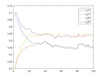
Figure 2: True opinion $v[k]$ when $\gamma=0.8$. Here both players are rational and risk-averse. Both players are doing R-learning to learn the behavior of their opponents.

V Real world applications

Deciding equity distribution is a critical step in forming a startup company [18]. For a long period of time, it has been regarded as a problem that is often solved case by case relying on experience. For example, [18] suggests that equity distribution should consider “past and future contributions,” but those contributions are very subjective. To avoid this subjectivity, [19] argues that everyone who joins the startup at the same time should receive equal shares.

Recent years there are some theories and practices trying to deal with this problem in a systematic way. To date, the most suitable theory is the Shapley value in coalitional game theory, in which payoffs are distributed according to the contribution of each of the sub-coalitions and the three axioms of fairness [20]. An online tool, “Startup Equity Calculator,” [21] implements this idea by asking the question “What will the company look like without this particular founder?”, which essentially evaluates the contribution of each of the sub-coalitions.

However, the above ideas of the Shapley value assume that everyone will agree on the contribution of each of the sub-coalitions. In practice, different people have different opinions about the contribution of each of the sub-coalitions, hence a coalitional game theory with incomplete information is required, such as the one in this paper.

As another example, in the United States, passing legislation requires substantial effort and extensive lobbying and debates, and the same game is not played repeatedly. Thus, a repeated game model in the paper [12] is not applicable. In contemporary U.S. politics, in addition, it is usually the case that the Bayesian core, defined in [5] does not exist, because the two parties have strong prejudices about each other. Moreover, the opinion exchange process affects the outcomes substantially, so a model, such as an opinion consensus model, is required to capture its effect. At the end, each Senator and Representative has her or his own interests and cares almost exclusively about the welfare of his or her own constituents.

VI Conclusions and Future work

In this paper, a new framework for coalitional games is presented with an unrealized subset payoff function and information exchange among players. The framework creates an interplay between the traditional model of the coalitional game and the opinion consensus model. Many interesting implications arise from the new framework, including the sufficient condition of non-stable core and the sufficient condition of efficient information exchange. Furthermore, the case of algorithmic learning players was studied, and the results were compared and connected to the case of pure rational players.

In the future, the dependency of equilibrium on the topology of the opinion consensus network may be considered. It is clear that different communication topologies will result in different steady states. From the perspective of an investor in the business scenario, there is a need to design a communication topology and rule (mechanism) that ensures truth telling. From the perspective of the participants, questions may arise concerning with whom and in what order should issues be addressed to ensure favorable outcomes. Additional future work that is needed is related to algorithmic learning. In this approach, quantizing the rewards associated with the possible “exit” action of each player also could be considered.

References

- [1] O. Shehory and S. Kraus, “Methods for task allocation via agent coalition formation,” Artificial Intelligence, vol. 101, no. 1, pp. 165–200, 1998.
- [2] W. Saad, Z. Han, H. V. Poor, and T. Basar, “Game-theoretic methods for the smart grid: An overview of microgrid systems, demand-side management, and smart grid communications,” IEEE Signal Processing Magazine, vol. 29, no. 5, pp. 86–105, 2012.
- [3] W. Saad, Z. Han, A. Hjorungnes, D. Niyato, and E. Hossain, “Coalition formation games for distributed cooperation among roadside units in vehicular networks,” IEEE Journal on Selected Areas in Communications, vol. 29, no. 1, pp. 48–60, 2011.
- [4] B. Jiang, A. N. Bishop, B. D. Anderson, and S. P. Drake, “Optimal path planning and sensor placement for mobile target detection,” Automatica, vol. 60, pp. 127–139, 2015.
- [5] S. Ieong and Y. Shoham, “Bayesian coalitional games.” in AAAI, 2008, pp. 95–100.
- [6] D. J. Hooper, “Coalition formation under uncertainty,” DTIC Document, Tech. Rep., 2010.
- [7] G. Chalkiadakis and C. Boutilier, “Sequentially optimal repeated coalition formation under uncertainty,” Autonomous Agents and Multi-Agent Systems, vol. 24, no. 3, pp. 441–484, 2012.
- [8] G. Chalkiadakis, E. Markakis, and C. Boutilier, “Coalition formation under uncertainty: Bargaining equilibria and the bayesian core stability concept,” in Proceedings of the 6th international joint conference on Autonomous agents and multiagent systems. ACM, 2007, p. 64.
- [9] J. Chapman, “The power of propaganda,” Journal of Contemporary History, vol. 35, no. 4, pp. 679–688, 2000.
- [10] G. Albi, L. Pareschi, and M. Zanella, “Boltzmann-type control of opinion consensus through leaders,” Philosophical Transactions of the Royal Society of London A: Mathematical, Physical and Engineering Sciences, vol. 372, no. 2028, p. 20140138, 2014.
- [11] B. Jiang, M. Roozbehani, and M. A. Dahleh, “Coalitional game with opinion exchange,” CoRR, vol. abs/1709.01432, 2017. [Online]. Available: https://arxiv.org/abs/1709.01432
- [12] G. Chalkiadakis and C. Boutilier, “Bayesian reinforcement learning for coalition formation under uncertainty,” in Proceedings of the Third International Joint Conference on Autonomous Agents and Multiagent Systems-Volume 3. IEEE Computer Society, 2004, pp. 1090–1097.
- [13] B. Jiang, M. Deghat, and B. D. Anderson, “Simultaneous velocity and position estimation via distance-only measurements with application to multi-agent system control,” IEEE Transactions on Automatic Control, vol. 62, no. 2, pp. 869–875, 2017.
- [14] T. Tanaka, F. Farokhi, and C. Langbort, “Faithful implementations of distributed algorithms and control laws,” IEEE Transactions on Control of Network Systems, vol. 4, no. 2, pp. 191–201, 2017.
- [15] J. Farrell, “Cheap talk, coordination, and entry,” The RAND Journal of Economics, pp. 34–39, 1987.
- [16] C. F. Camerer, T.-H. Ho, and J.-K. Chong, “A cognitive hierarchy model of games,” The Quarterly Journal of Economics, pp. 861–898, 2004.
- [17] R. S. Sutton and A. G. Barto, Reinforcement learning: An introduction. MIT press Cambridge, 1998, vol. 1, no. 1.
- [18] D. Rose and C. Patterson, Research to Revenue: A Practical Guide to University Start-ups. UNC Press Books, 2016.
- [19] J. Spolsky, “Where twitter and facebook went wrong — a fair way to divide up ownership of any new company,” Apr 2011. [Online]. Available: http://www.businessinsider.com/how-to-allocate-ownership-fairly-when-forming-a-new-software-startup-2011-4
- [20] L. S. Shapley, “A value for n-person games,” The Shapley value, pp. 31–40, 1988.
- [21] A. HA, “Foundrs.com: Find co-founders, don’t get screwed,” Oct 2010. [Online]. Available: http://venturebeat.com/2010/10/22/foundrs-com-find-co-founders-dont-get-screwed/