GPDs from charged current meson production in $ep$ experiments

Abstract

We suggest that generalized parton distributions can be probed in charged current meson production process, $ep\to\nu_{e}\pi^{-}p$. In contrast to pion photoproduction, this process is sensitive to the unpolarized GPDs $H,\,E$, and for this reason has a very small contamination by higher twist and Bethe-Heitler type contributions. Since all produced hadrons are charged, we expect that the kinematics of this process could be easily reconstructed. We estimated the cross-sections in the kinematics of upgraded 12 GeV Jefferson Laboratory experiments and found that thanks to large luminosity the process can be measured with reasonable statistics.

I Introduction

Understanding the structure of the hadrons presents a challenging problem both from the theoretical and experimental viewpoints. This structure is parametrized nowadays in terms of the so-called generalized parton distributions (GPDs), which can be studied in a wide class of processes Ji:1998xh ; Collins:1998be . The early analysis were mostly based on experimental data on deeply virtual Compton scattering (DVCS) Dupre:2017hfs and deeply virtual meson production (DVMP) Ji:1998xh ; Collins:1998be ; Mueller:1998fv ; Ji:1996nm ; Ji:1998pc ; Radyushkin:1996nd ; Radyushkin:1997ki ; Radyushkin:2000uy ; Collins:1996fb ; Brodsky:1994kf ; Goeke:2001tz ; Diehl:2000xz ; Belitsky:2001ns ; Diehl:2003ny ; Belitsky:2005qn ; Kubarovsky:2011zz , although it was soon realized that in view of the rich structure of GPDs, as well as from certain complications with GPD extraction from pion electroproduction Kubarovsky:2011zz ; Ahmad:2008hp ; Goloskokov:2009ia ; Goloskokov:2011rd ; Goldstein:2012az , additional channels were needed. It was then suggested that GPDs might be accessed in $\rho$-meson photoproduction Anikin:2009bf ; Diehl:1998pd ; Mankiewicz:1998kg ; Mankiewicz:1999tt ; Boussarie:2017umz , timelike Compton Scattering Berger:2001xd ; Pire:2008ea ; Boer:2015fwa , exclusive pion- or photon-induced lepton pair production Muller:2012yq ; Sawada:2016mao , and heavy charmonia photoproduction Ivanov:2004vd ; Ivanov:2015hca (gluon GPDs). The forthcoming results from the upgraded JLAB Kubarovsky:2011zz , COMPASS Gautheron:2010wva ; Kouznetsov:2016vvo ; Ferrero:2012ega ; Sandacz:2016kwh ; Sandacz:2017ctv ; Silva:2013dta as well as from J-PARC Sawada:2016mao ; Kroll:2016kvd , hopefully will enrich and enhance the early data from HERA and 6 GeV JLab experiments, as well as improve our understanding of the proton GPDs.

Recently we suggested that GPDs could be studied in neutrino-induced deeply virtual meson production ($\nu$DVMP) Kopeliovich:2012dr of the pseudoscalar mesons ($\pi,\,K,\,\eta$), using the high-intensity NuMI beam at Fermilab Drakoulakos:2004gn . The main advantage of this process is that contamination by twist-3 effects Kopeliovich:2014pea is small, which implies that GPDs could be accessed at moderate virtualities $Q^{2}$, provided that the next-to-leading order (NLO) corrections are included Siddikov:2016zmt . In the Bjorken limit, neglecting the masses of pions and kaons, we may get information about a full flavor structure of GPDs. A suppression of Cabibbo forbidden, strangeness changing processes can be avoided if kaon production is accompanied by the conversion of a nucleon to strange baryons $\Lambda$ and $\Sigma^{\pm,0}$; in such processes the transition GPDs are related by $SU(3)$ relations Frankfurt:1999fp to linear combinations of different flavor components of the nucleon GPDs. Recently it was suggested in Pire:2015iza ; Pire:2015vxa ; Pire:2016jtr ; Pire:2017lfj ; Pire:2017tvv that this approach could be extended to $D$-meson production, a challenge for future high-energy neutrino experiments.

In this paper we extend our previous studies to the case of charged current meson (pion) production in electron-induced processes, such as e.g. $ep\to\nu_{e}\pi^{-}p$. The feasibility to study charged currents in JLAB kinematics has been demonstrated earlier in Androic:2013rhu . It is expected that after upgrade even higher luminosities up to $\mathcal{L}=10^{38}{\rm cm}^{-2}\cdot s^{-1}$ will be achieved Alcorn:2004sb , which implies that the DVMP cross-section could be measured with reasonable statistics. Since all produced hadrons are charged, the reconstruction of the kinematics of the process, despite of undetectability of neutrinos, should not present major difficulties. As will be shown below, the cross-section of this process on unpolarized targets is mostly sensitive to the GPDs $H_{u},\,H_{d}$, providing important constraints on available parametrizations, as well as testing the GPD universality. Similar to the case of neutrino-production, this process has smaller contamination by higher twist effects compared to DVMP.

For the sake of brevity and conciseness, in this paper we do not consider other processes, where flavor multiplet partners of pions and protons are produced and which could be used to test other flavor combinations of GPDs Kopeliovich:2012dr .

The paper is organized as follows. In Section II we describe the framework used for the evaluation of pion production, taking into account NLO corrections. In Sections III and IV we review the contaminating corrections due to Bethe-Heitler mechanism and twist-three contributions, due to poorly known transversity GPDs. Finally, in Section V we present numerical results and make conclusions.

II Cross-section of the $\nu$DVMP process

The cross-section of pion production in charged current DVMP has a form

$$\frac{d\sigma}{dt\,dx_{B}dQ^{2}} =\Gamma\sum_{\nu\nu^{\prime}}\mathcal{A}_{\nu^{\prime},\nu L}^{*}\mathcal{A}_{\nu^{\prime},\nu L},$$ (1)

where $t=\left(p_{2}-p_{1}\right)^{2}$ is the momentum transfer to the proton, $Q^{2}=-q^{2}$ is the virtuality of the charged boson, $x_{B}=Q^{2}/(2p\cdot q)$ is the Bjorken variable, the subscript indices $\nu$ and $\nu^{\prime}$ in the amplitude $\mathcal{A}$ refer to helicity states of the baryon before and after interaction, and the letter $L$ reflects the fact that in the Bjorken limit the dominant contribution comes from the longitudinally polarized massive bosons $W^{\pm}$ Ji:1998xh ; Collins:1998be . The kinematic factor $\Gamma$ included in equation (1) is given explicitly, for the charged current case, by

$$\Gamma =\frac{G_{F}^{2}f_{M}^{2}x_{B}^{2}\left(1-y-\frac{\gamma^{2}y^{2}}{4}\right)}{64\pi^{3}Q^{2}\left(1+Q^{2}/M_{W}^{2}\right)^{2}\left(1+\gamma^{2}\right)^{3/2}},$$ (2)

where $\theta_{W}$ is the Weinberg angle, $M_{W}$ is the mass of the heavy bosons $W^{\pm}$, $G_{F}$ is the Fermi constant, $f_{\pi}$ is the pion decay constant, and we used the shorthand notations

$$\gamma=\frac{2\,m_{N}x_{B}}{Q},\quad y=\frac{Q^{2}}{s_{ep}\,x_{B}}=\frac{Q^{2}}{2m_{N}E_{e}\,x_{B}}.$$ (3)

where $E_{e}$ is the electron energy in the target rest frame. In Bjorken kinematics, the amplitude $\mathcal{A}_{\nu^{\prime},\nu L}$ factorizes into a convolution of hard and soft parts,

$$\mathcal{A}_{\nu^{\prime},\nu}=\int_{-1}^{+1}dx\sum_{q=u,d,s,g}\,\sum_{\lambda\lambda^{\prime}}\mathcal{H}_{\nu^{\prime}\lambda^{\prime},\nu\lambda}^{q}\mathcal{C}_{\lambda\lambda^{\prime}}^{q},$$ (4)

where $x$ is the average light-cone fraction of the parton, the superscript $q$ is its flavor, $\lambda$ and $\lambda^{\prime}$ are the helicities of the initial and final partons, and $\mathcal{C}_{\lambda^{\prime}\nu^{\prime},\lambda\nu}^{q}$ is the hard coefficient function, which will be specified later. The soft matrix element $\mathcal{H}_{\nu^{\prime}\lambda^{\prime},\nu\lambda}^{q}$ in (11) is diagonal in quark helicities ($\lambda,\,\lambda^{\prime}$), and for the twist-2 GPDs has the form,

$$\mathcal{H}_{\nu^{\prime}\lambda^{\prime},\nu\lambda}^{q} =\frac{2\delta_{\lambda\lambda^{\prime}}}{\sqrt{1-\xi^{2}}}\left(-g_{A}^{q}\left(\begin{array}[]{cc}\left(1-\xi^{2}\right)H^{q}-\xi^{2}E^{q}&\frac{\left(\Delta_{1}+i\Delta_{2}\right)E^{q}}{2m}\\ -\frac{\left(\Delta_{1}-i\Delta_{2}\right)E^{q}}{2m}&\left(1-\xi^{2}\right)H^{q}-\xi^{2}E^{q}\end{array}\right)_{\nu^{\prime}\nu}\right.$$ (7)

$$+\left.{\rm sgn}(\lambda)g_{V}^{q}\left(\begin{array}[]{cc}-\left(1-\xi^{2}\right)\tilde{H}^{q}+\xi^{2}\tilde{E}^{q}&\frac{\left(\Delta_{1}+i\Delta_{2}\right)\xi\tilde{E}^{q}}{2m}\\ \frac{\left(\Delta_{1}-i\Delta_{2}\right)\xi\tilde{E}^{q}}{2m}&\left(1-\xi^{2}\right)\tilde{H}^{q}-\xi^{2}\tilde{E}^{q}\end{array}\right)_{\nu^{\prime}\nu}\right),$$ (10)

where the constants $g_{V}^{q},\,g_{A}^{q}$ are the vector and axial current couplings to quarks, and the leading twist GPDs $H^{q},\,E^{q},\,\tilde{H}^{q}$ and $\tilde{E}^{q}$ are functions of the variables $\left(x,\,\xi,\,t,\,\mu_{F}^{2}\right)$, where the skewness $\xi$ is related to the light-cone momenta of protons $p_{1,2}$ as $\xi=\left(p_{1}^{+}-p_{2}^{+}\right)/\left(p_{1}^{+}+p_{2}^{+}\right)$, the invariant momentum transfer is $t=\Delta^{2}=\left(p_{2}-p_{1}\right)^{2}$, and $\mu_{F}$ is the factorization scale (see e.g. Goeke:2001tz ; Diehl:2003ny for details of the kinematics). For the processes in which the baryonic state changes, e.g. $ep\to\nu_{e}\pi_{0}n$, the transition GPDs can be linearly related via $SU(3)$ relations Frankfurt:1999fp to ordinary GPDs. For this reason, (4) may be effectively rewritten as

$$\mathcal{A}_{\nu^{\prime},\nu}=\int_{-1}^{+1}dx\sum_{q=u,d,s}\,\sum_{\lambda}\mathcal{H}_{\nu^{\prime}\lambda,\nu\lambda}^{q}\mathcal{C}_{\lambda}^{q}.$$ (11)

where $\mathcal{C}_{\lambda}^{q}$ is the diagonal term of the helicity matrix in the hard coefficient function. Its evaluation is quite straightforward, and in leading order over $\alpha_{s}$ it gets contributions from the diagrams shown schematically in Figure 1. In fact, it has been studied both for pion electroproduction Vanderhaeghen:1998uc ; Mankiewicz:1998kg ; Goloskokov:2006hr ; Goloskokov:2007nt ; Goloskokov:2008ib ; Goloskokov:2011rd ; Goldstein:2012az and neutrinoproduction Kopeliovich:2012dr . For the processes in which the baryon does not change its internal state, there are additional contributions from gluon GPDs, as shown in the rightmost pane of Figure 1. These corrections are small for JLAB kinematics, yet give a contributions at higher energies. In next-to-leading order, the coefficient function includes an additional gluon attached in all possible ways to all diagrams in Figure 1, as well as additional contributions from sea quarks, as shown in Figure 2.

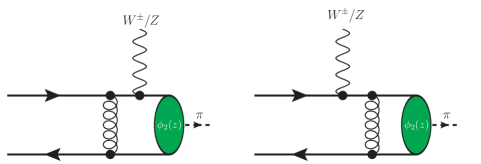
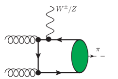
Figure 1: Leading-order contributions to the DVMP hard coefficient functions. Green blob stands for the pion wave function. Additional diagrams (not shown) may be obtained reversing the directions of the quark lines and in the case of the last diagram, permuting also the vector boson vertices.

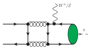
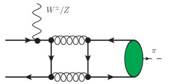
Figure 2: Sea quark contributions to the DVMP, which appear in the next-to-leading-order contributions. Additional diagrams (not shown) may be obtained by reversing the directions of the quark lines.

Straightforward evaluation of the diagrams shown in the Figures 1,2 yields for the coefficient functions

$$\mathcal{C}^{q} =\eta_{-}^{q}c_{-}^{(q)}\left(x,\,\xi\right)+{\rm sgn}(\lambda)\eta_{+}^{q}c_{+}^{(q)}\left(x,\,\xi\right)+\mathcal{O}\left(\frac{m^{2}}{Q^{2}}\right)+\mathcal{O}\left(\alpha_{s}^{2}\left(\mu_{R}^{2}\right)\right)$$ (12)

where the process-dependent flavor factors $\eta_{V\pm}^{q},\,\eta_{A\pm}^{q}$ are given, for the case of pion production, in Table 1 . In (12) we also introduced the shorthand notation

Table 1: The flavor coefficients $\eta_{\pm}^{q}$, for several pion and kaon production processes discussed in this paper ($q=u,d,s,...$). For the case of CC mediated processes, take $\eta_{V\pm}^{q}=\eta_{\pm}^{q},\quad\eta_{A\pm}^{q}=-\eta_{\pm}^{q}$.

Process	$\eta_{+}^{q}$	$\eta_{-}^{q}$		Process	$\eta_{+}^{q}$	$\eta_{-}^{q}$
$e\,p\to\nu_{e}\pi^{-}p$	$V_{ud}\delta_{qd}$	$V_{ud}\delta_{qu}$		$e\,p\to\nu_{e}\pi^{0}n$	$V_{ud}\frac{\delta_{qu}-\delta_{qd}}{\sqrt{2}}$	$-V_{ud}\frac{\delta_{qu}-\delta_{qd}}{\sqrt{2}}$
$e\,p\to\nu_{e}\pi^{0}n$	$V_{ud}\frac{\delta_{qu}-\delta_{qd}}{\sqrt{2}}$	$-V_{ud}\frac{\delta_{qu}-\delta_{qd}}{\sqrt{2}}$		$e\,n\to\nu_{e}\pi^{-}n$	$V_{ud}\delta_{qu}$	$V_{ud}\delta_{qd}$
$e\,p\to\nu_{e}K^{-}p$	$V_{us}\delta_{qs}$	$V_{us}\delta_{qs}$		$e\,n\to\nu_{e}K^{0}\Sigma^{-}$	0	$-V_{ud}\left(\delta_{qu}-\delta_{qs}\right)$

$$c_{\pm}^{(q)}\left(x,\xi\right) = \left(\int dz\frac{\phi_{2,\pi}\left(z\right)}{z}\right)\frac{8\pi i}{9}\frac{\alpha_{s}\left(\mu_{R}^{2}\right)f_{M}}{Q}\frac{1}{x\pm\xi\mp i0}\left(1+\frac{\alpha_{s}\left(\mu_{r}^{2}\right)}{2\pi}T^{(1)}\left(\frac{\xi\pm x}{2\xi},\,z\right)\right).$$ (13)

where $\phi_{2}(z)$ is the twist-2 $\pi-$or $K$-meson distribution amplitude (DA) Kopeliovich:2011rv . The function $T^{(1)}\left(v,\,z\right)$ in (13) encodes NLO corrections to the coefficient function. As was explained in Belitsky:2001nq ; Ivanov:2004zv ; Diehl:2007hd , it is related by analytical continuation to the loop correction to $\bar{q}q$ scattering, and was evaluated and analyzed in detail in the context of NLO studies of the pion form factor (see Braaten:1987yy ; Melic:1998qr for details and historical discussion). Explicitly, it is given by

$$T^{(1)}\left(v,\,z\right) =\frac{1}{2vz}\left[\frac{4}{3}\left([3+\ln(v\,z)]\,\ln\left(\frac{Q^{2}}{\mu_{F}^{2}}\right)+\frac{1}{2}\ln^{2}\left(v\,z\right)+3\ln(v\,z)-\frac{\ln\bar{v}}{2\bar{v}}-\frac{\ln\bar{z}}{2\bar{z}}-\frac{14}{3}\right)\right.$$ (14)

$$+\beta_{0}\left(\frac{5}{3}-\ln(v\,z)-\ln\left(\frac{Q^{2}}{\mu_{R}^{2}}\right)\right)$$

$$-\frac{1}{6}\left(2\frac{\bar{v}\,v^{2}+\bar{z}\,z^{2}}{(v-z)^{3}}\left[{\rm Li}_{2}(\bar{z})-{\rm Li}_{2}(\bar{v})+{\rm Li}_{2}(v)-{\rm Li}_{2}(z)+\ln\bar{v}\,\ln z-\ln\bar{z}\,\ln v\right]\right.$$

$$+2\frac{v+z-2v\,z}{(v-z)^{2}}\ln\left(\bar{v}\bar{z}\right)+2\left[{\rm Li}_{2}(\bar{z})+{\rm Li}_{2}(\bar{v})-{\rm Li}_{2}(z)-{\rm Li}_{2}(v)+\ln\bar{v}\,\ln z+\ln\bar{z}\,\ln v\right]$$

$$+\left.\left.4\frac{v\,z\,\ln(v\,z)}{(v-z)^{2}}-4\ln\bar{v}\,\ln\bar{z}-\frac{20}{3}\right)\right],$$

where $\beta_{0}=\frac{11}{3}N_{c}-\frac{2}{3}N_{f}$, ${\rm Li}_{2}(z)$ is the dilogarithm function, and $\mu_{R}$ and $\mu_{F}$ are the renormalization and factorization scales respectively. For processes when the internal state of the hadron is not changed, additional contributions come from the gluons and singlet (sea) quarks Belitsky:2001nq ; Ivanov:2004zv ; Diehl:2007hd  ,

$$c^{(g)}\left(x,\xi\right) = \left(\int dz\frac{\phi_{2,\pi}\left(z\right)}{z\,(1-z)}\right)\frac{2\pi i}{3}\frac{\alpha_{s}\left(\mu_{R}^{2}\right)f_{M}}{Q}\frac{\xi}{\left(\xi+x-i0\right)\left(\xi-x-i0\right)}\left(1+\frac{\alpha_{s}\left(\mu_{r}^{2}\right)}{4\pi}\mathcal{I}^{(g)}\left(\frac{\xi-x}{2\xi},\,z\right)\right),$$ (15)

$$\mathcal{I}^{(g)}\left(v,\,z\right) = \left(\ln\left(\frac{Q^{2}}{\mu_{F}^{2}}\right)-1\right)\left[\frac{\beta_{0}}{2}+C_{A}\left[\left(1-v\right)^{2}+v^{2}\right]\left(\frac{\ln\left(1-v\right)}{v}+\frac{\ln v}{1-v}\right)-\frac{C_{F}}{2}\left(\frac{v\ln v}{1-v}+\frac{\left(1-v\right)\ln\left(1-v\right)}{v}\right)\right.$$

$$+\left.C_{F}\left(\frac{3}{2}+2\,z\ln\left(1-z\right)\right)\right]-2\,C_{F}-\frac{\beta_{0}}{2}\left(\ln\left(\frac{Q^{2}}{\mu_{R}^{2}}\right)-1\right)-\frac{C_{F}\left(1-2\,v\right)}{2\,\left(z-v\right)}R\left(z,\,v\right)$$

$$+\frac{\left(2C_{A}-C_{F}\right)}{4}\left(\frac{v\,\ln^{2}v}{1-v}+\frac{\left(1-v\right)\ln^{2}\left(1-v\right)}{v}\right)+C_{F}(1+3\,z)\ln\left(1-z\right)+$$

$$+\left(\ln\,v+\ln\left(1-v\right)\right)\left[C_{F}\left(1-z\right)\ln\,z-\frac{1}{4}+2C_{F}-C_{A}\right]$$

$$+\frac{C_{A}}{2}\left(\ln\left(z\,(1-z)\right)-2\right)\left[\frac{v\,\ln v}{1-v}+\frac{\left(1-v\right)\,\ln\left(1-v\right)}{v}\right]$$

$$+C_{F}z\,\ln^{2}\left(1-z\right)+\frac{C_{A}}{2}\left(1-2\,v\right)\ln\left(\frac{v}{1-v}\right)\left[\frac{3}{2}+\ln\left(z\,\left(1-z\right)\right)+\ln\left(v\,\left(1-v\right)\right)\right]$$

$$+\left(C_{F}\left((z-v)^{2}-v\,(1-v)\right)-\left(C_{F}-\frac{C_{A}}{2}\right)(z-v)(1-2v)\right)\times$$

$$\times\left[-\frac{R(z,v)}{(z-v)^{2}}+\frac{\ln v+\ln z-\ln\left(1-v\right)-\ln\left(1-z\right)}{2\left(z-v\right)}+\frac{(z-v)^{2}-v(1-v)}{(z-v)^{3}}H(z,v)\right]$$

$$+\left\{\frac{}{}z\to 1-z\right\},$$

$$C_{F} = \frac{N_{c}^{2}-1}{2N_{c}},\quad C_{A}=N_{c}.$$ (17)

$$c_{\pm}^{(s)}\left(x,\xi\right) = -\left(\int dz\frac{\phi_{2,\pi}\left(z\right)}{z\,(1-z)}\right)\frac{4i\alpha_{s}^{2}\left(\mu_{R}^{2}\right)f_{M}}{9\,Q}\mathcal{I}^{(s)}\left(\frac{x\pm\xi}{2\xi},\,z\right),$$ (18)

$$\mathcal{I}^{(s)}\left(v,\,z\right) = \left(1-2\,v\right)\left(\frac{\ln v}{1-v}+\frac{\ln(1-v)}{v}\right)\ln\left(\frac{Q^{2}z}{\mu_{F}^{2}}\right)+\frac{1-2v}{2}\left[\frac{\ln^{2}v}{1-v}+\frac{\ln^{2}\left(1-v\right)}{v}\right]$$

$$-\frac{R(v,\,z)}{z-v}-\frac{\left(1-v\right)\ln\left(1-v\right)-v\ln v}{v\left(1-v\right)}+\frac{\left(z-v\right)^{2}-v\left(1-v\right)}{\left(z-v\right)^{2}}H\left(v,z\right)+\left\{\frac{}{}z\to 1-z\right\},$$

$$R\left(v,\,z\right) = z\ln v+(1-z)\,\ln\left(1-v\right)+z\,\ln z+\left(1-v\right)\ln\left(1-v\right),$$ (20)

$$H\left(v,\,z\right) = {\rm Li}_{2}\left(1-v\right)-{\rm Li}_{2}\left(v\right)+{\rm Li}_{2}\left(z\right)-{\rm Li}_{2}\left(1-z\right)+\ln v\,\ln\left(1-z\right)-\ln\left(1-v\right)\ln\,z.$$ (21)

Some coefficient functions have non-analytic behavior $\sim\ln^{2}v$ for small $v\approx 0$ ($x=\pm\xi\mp i0$), which signals that a collinear approximation might be not valid near this point. This singularity in the collinear limit occurs due to the omission of the small transverse momentum $l_{M,\perp}$ of the quark inside a meson Goloskokov:2009ia , and for this reason the contribution of the region $|v|\sim l_{M,\perp}^{2}/Q^{2}$ should be treated with due care for finite $Q^{2}$ (beyond the Bjorken limit). Moreover, a full evaluation of $T^{(1)}\left(v,\,z\right)$ beyond the collinear approximation (taking into account all higher twist corrections) presents a challenging problem and has not been done so far. It was observed in Diehl:2007hd , that the singular terms might be eliminated by a redefinition of the renormalization scale $\mu_{R}$; however, near the point $v\approx 0$ the scale $\mu_{R}^{2}$ becomes soft, $\mu_{R}^{2}\sim z\,v\,Q^{2}\lesssim l_{\perp}^{2}$, which is another manifestation that nonperturbative effects become relevant. For this reason, sufficiently large value of $Q^{2}$ should be used to mitigate contributions of higher twist effects. As we will see below, for $Q^{2}\approx 4$ GeV² the contribution of this soft region is small, so the collinear factorization is reliable.

III Bethe-Heitler type contribution

As was found in Ref. Kopeliovich:2013ae , in the asymptotic Bjorken limit ($Q^{2}\to\infty$) the DVMP contribution gets overwhelmed by subleading $\mathcal{O}\left(\alpha_{em}\right)$ Bethe-Heitler type (BH) contributions, shown in Figure 3. These diagrams have milder suppression at large $Q^{2}$ compared to DVMP and are additionally enhanced by the $t$-channel photon pole $\sim 1/t$ in the forward kinematics, and for this reason at sufficiently large $\sim Q^{2}/t$ this mechanism becomes dominant.

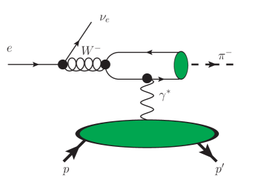
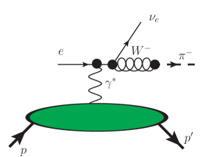
Figure 3: Bethe-Heitler contribution in the charged current DVMP. Formally it is suppressed as $\mathcal{O}\left(\alpha_{{\rm em}}\right)$ compared to DVMP contribution; however, for the asymptotic Bjorken limit it becomes the dominant mechanism due to relative enhancement by a kinematical factor $\sim Q^{2}/t\,\alpha_{s}(Q^{2})$. The green blob stands for the pion wave function.

While for the DVMP amplitude evaluation presented in the previous section the dominant contribution comes from the longitudinally polarized mediator boson, for the BH this is no longer true and we have to consider all the $W$ polarizations. The left diagram in Figure 3 contains the matrix element

$$\mathcal{A}_{\mu\nu}^{ab}\left(q,\Delta\right)=\frac{1}{f_{\pi}}\int d^{4}x\,e^{-iq\cdot x}\left\langle 0\left|\left(V_{\mu}^{a}(x)-A_{\mu}^{a}(x)\right)J_{\nu}^{em}(0)\right|\pi^{b}\left(q-\Delta\right)\right\rangle,$$ (22)

where $V_{\mu}^{a}(x)$ and $A_{\mu}^{a}(x)$ are the vector and axial isovector currents. We evaluate the correlator (22) perturbatively in the collinear approximation, which is justified by the intermediate boson large $Q^{2}$ value, and therefore consider only the dominant contribution from the leading twist-2 pion DA. The evaluation details may be found in Kopeliovich:2013ae , while here for the sake of brevity we will only provide the final result. The cross-section of the Bethe-Heitler mechanism is given by

$$\frac{d^{4}\sigma^{(BH)}}{dt\,d\ln x_{Bj}\,dQ^{2}d\varphi}=\frac{f_{\pi}^{2}G_{F}^{2}\alpha_{em}^{2}\sum_{n=0}^{2}\mathcal{C}_{n}^{BH}\cos(n\varphi)}{16\,\pi^{2}t^{2}\left(1+\frac{4m_{N}^{2}x_{B}^{2}}{Q^{2}}\right)^{5/2}},$$ (23)

where $\varphi$ is the angle between the lepton scattering and the pion production planes, and in addition to the kinematic variables defined in the previous section II we introduced shorthand notations

$$\mathcal{C}_{0}^{BH} =\mathcal{C}_{2}^{BH}+\frac{m_{N}^{2}}{9\,Q^{2}}\left[4\left(\left(2y^{2}+y-1\right)\left(\phi_{-1}-1\right)x_{B}^{3}\right.\right.$$ (24)

$$-\left(\left(4\left(\phi_{-1}-1\right)^{2}+\frac{t}{2m_{N}^{2}}\left(4\phi_{-1}^{2}-8\phi_{-1}+5\right)\right)y^{2}-4\left(\left(\phi_{-1}-1\right)^{2}+\frac{t}{4m_{N}^{2}}\left(4\phi_{-1}^{2}-13\phi_{-1}+10\right)\right)y\right.$$

$$+\left.\frac{5t}{2m_{N}^{2}}\left(\phi_{-1}-2\right)^{2}+\left(\phi_{-1}-1\right)^{2}\right)x_{B}^{2}+\left(2y-1\right)\frac{t}{m_{N}^{2}}\left(\phi_{-1}-1\right)\left(-\phi_{-1}+y\left(2\phi_{-1}-1\right)+2\right)x_{B}$$

$$-\left.4\left(1-2y\right)^{2}\frac{t}{4m_{N}^{2}}\left(\phi_{-1}-1\right)^{2}\right)F_{1}^{2}(t)+2F_{1}(t)F_{2}(t)x_{B}^{2}\left(x_{B}^{2}\left(y+1\right)^{2}-\frac{x_{B}t}{m_{N}^{2}}\left(y+1\right)^{2}\right.$$

$$\left.-\frac{t}{m_{N}^{2}}\left(\left(8\phi_{-1}^{2}-24\phi_{-1}+17\right)y^{2}-2\left(8\phi_{-1}^{2}-24\phi_{-1}+19\right)y+10\phi_{-1}^{2}-36\phi_{-1}+35\right)\right)$$

$$+F_{2}^{2}\left(\left(y+1\right)^{2}\left(\frac{t}{4m_{N}^{2}}+1\right)x_{B}^{4}-\left(y+1\right)\frac{t}{m_{N}^{2}}\left(\frac{t}{4m_{N}^{2}}-\phi_{-1}+y\left(\frac{t}{4m_{N}^{2}}+2\phi_{-1}-1\right)+2\right)x_{B}^{3}\right.$$

$$+\frac{t\,x_{B}^{2}}{m_{N}^{2}}\left(\left(-4\phi_{-1}^{2}+16\phi_{-1}+\frac{t}{4m_{N}^{2}}\left(8\phi_{-1}-7\right)-13\right)y^{2}\right.$$

$$\left.+2\left(6\phi_{-1}^{2}-20\phi_{-1}+\frac{t}{4m_{N}^{2}}\left(2\phi_{-1}-1\right)+17\right)y-9\phi_{-1}^{2}+\frac{t}{4m_{N}^{2}}\left(5-4\phi_{-1}\right)+34\phi_{-1}-34\right)$$

$$\left.\left.-\left(2y-1\right)\left(\frac{t}{m_{N}^{2}}\right)^{2}\left(\phi_{-1}-1\right)\left(-\phi_{-1}+y\left(2\phi_{-1}-1\right)+2\right)x_{B}+\left(1-2y\right)^{2}\left(\frac{t}{4m_{N}^{2}}\right)^{2}\left(\phi_{-1}-1\right)^{2}\right)\right]$$

$$+\mathcal{O}\left(\frac{m_{N}^{4}}{Q^{4}},\frac{t^{2}}{Q^{4}}\right),$$

$$\mathcal{C}_{1}^{BH} =\frac{K\,m_{N}^{2}}{9Q^{2}}\left[4\left(3\left(-4y+3\left(y-2\right)\phi_{-1}+9\right)x_{B}^{3}\right.\right.$$ (25)

$$-2\left(\phi_{-1}-1\right)\left(-\left(\frac{5t}{2m_{N}^{2}}+9\right)\phi_{-1}+2y\left(\frac{t\phi_{-1}}{m_{N}^{2}}-\frac{3t}{4m_{N}^{2}}+3\phi_{-1}-6\right)+18\right)x_{B}^{2}$$

$$+\left.\frac{3t}{m_{N}^{2}}\left(\phi_{-1}-1\right)\left(-6\phi_{-1}+y\left(4\phi_{-1}-3\right)+3\right)x_{B}-\left(2y-3\right)\frac{6\,t}{m_{N}^{2}}\left(\phi_{-1}-1\right)^{2}\right)F_{1}^{2}(t)$$

$$+4F_{1}(t)F_{2}(t)x_{B}^{2}\left(3\left(y-3\right)x_{B}^{2}-12\left(y-3\right)\frac{t}{4m_{N}^{2}}x_{B}-8\frac{t}{4m_{N}^{2}}\left(4y\left(\phi_{-1}-3\right)-5\phi_{-1}+18\right)\left(\phi_{-1}-1\right)\right)$$

$$-F_{2}^{2}(t)\left(-6\left(y-3\right)x_{B}^{4}\right.$$

$$+\frac{t}{4m_{N}^{2}}\left(-6\left(y-3\right)x_{B}^{2}+12\left(-2y+3\left(y-2\right)\phi_{-1}+3\right)x_{B}+8\left(2y\left(\phi_{-1}-6\right)-\phi_{-1}+18\right)\left(\phi_{-1}-1\right)\right)x_{B}^{2}$$

$$\left.\left.+24\left(\frac{t}{4m_{N}^{2}}\right)^{2}\left(x_{B}\left(x_{B}-2\phi_{-1}+2\right)+2\left(\phi_{-1}-1\right)\right)\left(x_{B}\left(y-3\right)-2\left(2y-3\right)\left(\phi_{-1}-1\right)\right)\right)\right]$$

$$+\mathcal{O}\left(\frac{m_{N}^{4}}{Q^{4}},\frac{t^{2}}{Q^{4}}\right)$$

$$\mathcal{C}_{2}^{BH} =-\frac{4\,K^{2}}{9}\left[\left(5x_{B}-4\phi_{-1}+4\right)\left(\phi_{-1}-1\right)F_{1}^{2}(t)+2x_{B}^{2}F_{1}(t)F_{2}(t)\right.$$ (26)

$$+\left.\left(\left(1+\frac{t}{4m_{N}^{2}}\right)x_{B}^{2}-\frac{5\,t\,x_{B}}{4m_{N}^{2}}\left(\phi_{-1}-1\right)+\frac{t}{m_{N}^{2}}\left(\phi_{-1}-1\right)^{2}\right)F_{2}^{2}(t)\right]$$

$$+\mathcal{O}\left(\frac{m_{N}^{2}}{Q^{2}},\,\frac{t}{Q^{2}}\right),$$

$$K^{2} =\frac{\Delta_{\perp}^{2}}{Q^{2}}\left(1-y-\frac{y^{2}\epsilon^{2}}{4}\right)$$ (27)

$$=-\frac{t}{Q^{2}}\left(1-x_{B}\right)\left(1-y-\frac{\epsilon^{2}y^{2}}{4}\right)\left(1-\frac{t_{min}}{t}\right)\left\{\sqrt{1+\epsilon^{2}}+\frac{4x_{B}\left(1-x_{B}\right)+\epsilon^{2}}{4\left(1-x_{B}\right)}\frac{t-t_{min}}{Q^{2}}\right\},$$

$$\epsilon^{2} =\frac{4m_{N}^{2}x_{B}^{2}}{Q^{2}},\quad t_{min}=-\frac{m_{N}^{2}x_{B}^{2}}{1-x_{B}}+\mathcal{O}\left(\frac{m_{N}^{2}}{Q^{2}},\frac{t}{Q^{2}}\right),\qquad\phi_{-1}=\int_{0}^{1}\,\frac{\phi_{2,\pi}(z)}{z}\,dz.$$ (28)

In the expressions (24-26) we use the notation $F_{1,2}(t)$ for the Dirac and Pauli form factors. As we can see, the BH cross-section is symmetric under the $\varphi\to-\varphi$ transformation. For asymptotically large $Q^{2}$, the $\mathcal{C}_{1}^{BH}$ harmonic is suppressed by $\Delta_{\perp}/Q$, whereas $\mathcal{C}_{0}^{BH}\sim\mathcal{C}_{2}^{BH}$, and therefore the distribution is also symmetric with respect to the $\varphi\to\pi-\varphi$ transformation.

The interference between the DVMP and BH amplitudes yields an additional contribution

$$\frac{d^{4}\sigma^{(int)}}{dt\,d\ln x_{Bj}\,dQ^{2}d\varphi} =\frac{f_{\pi}^{2}G_{F}^{2}\,x_{B}\alpha_{em}\alpha_{S}\phi_{-1}\left(\mathcal{C}_{0}^{int}+\mathcal{C}_{1}^{int}\cos\varphi+\mathcal{S}_{1}^{int}\sin\varphi\right)}{36\,\pi^{2}t\,Q^{2}\left(1-\frac{x_{B}}{2}\right)\left(1+\frac{4m_{N}^{2}x_{B}^{2}}{Q^{2}}\right)^{5/2}},$$ (29)

where

$$\mathcal{C}_{0}^{int} =-\frac{m_{N}^{2}(1-y)}{Q^{2}}\left(\left(-4\left(1-x_{B}\right)\Re e\mathcal{H}+x_{B}^{2}\,\Re e\mathcal{E}\right)F_{1}+\Re e\mathcal{E}\,F_{2}\frac{t}{4m_{N}^{2}}(x_{B}-2)^{2}+\left(\Re e\mathcal{H}+\Re e\mathcal{E}\right)F_{2}x_{B}^{2}\right)$$ (30)

$$\times\left(\left(2\phi_{-1}-3\right)x_{B}^{2}-\frac{t}{m_{N}^{2}}\left(\phi_{-1}-1\right)\left(1+x_{B}\right)\right)+\mathcal{O}\left(\frac{m_{N}^{2}}{Q^{2}},\frac{t}{Q^{2}}\right),$$

$$\mathcal{C}_{1}^{int} =\frac{K}{3}\,\left[F_{1}\left(2\,\mathcal{R}e\,\mathcal{E}\left(y-3\right)x_{B}^{2}+\mathcal{R}e\,\mathcal{H}\left(4\left(x_{B}-2\right)\left(2y-3\right)\phi_{-1}-4\left(\left(x_{B}-4\right)y+6\right)\right)\right)\right.$$ (31)

$$+F_{2}\left(2\,\mathcal{R}e\mathcal{H}\left(y-3\right)x_{B}^{2}+\mathcal{R}e\,\mathcal{E}\left(2x_{B}^{2}\left(y-3\right)-\left(x_{B}-2\right)\frac{t}{4m_{N}^{2}}\left(4\left(2y-3\right)\left(\phi_{-1}-1\right)-2x_{B}\left(y-3\right)\right)\right)\right)$$

$$+\left.\mathcal{O}\left(\frac{m_{N}^{2}}{Q^{2}},\frac{t}{Q^{2}}\right)\right]$$

$$\mathcal{S}_{1}^{int} =\frac{K\left(2-x_{B}\right)}{6}\,\left[F_{1}\left(-2\,\mathcal{I}m\,\mathcal{E}\left(y+1\right)x_{B}^{2}-2\,\mathcal{I}m\,\mathcal{H}\left(x_{B}\left(4\phi_{-1}y-2y-2\phi_{-1}+4\right)-4\left(2y-1\right)\left(\phi_{-1}-1\right)\right)\right)\right.$$ (32)

$$+F_{2}\left(-2\,\mathcal{I}m\,\mathcal{H}\left(y+1\right)x_{B}^{2}\right.$$

$$\left.-2\,\mathcal{I}m\,\mathcal{E}\left(\left(y+1\right)\left(1+\frac{t}{4m_{N}^{2}}\right)x_{B}^{2}+\frac{t}{2m_{N}^{2}}\left(-2\phi_{-1}y+y+\phi_{-1}-2\right)x_{B}+\left(2y-1\right)\frac{t}{m_{N}^{2}}\left(\phi_{-1}-1\right)\right)\right)$$

$$+\left.\mathcal{O}\left(\frac{m_{N}^{2}}{Q^{2}},\frac{t}{Q^{2}}\right)\right],$$

The angular dependence of the interference term (29) has a $\sim\sin\varphi$ term, which stems from the interference of the vector and axial vector currents in the lepton part of the diagram. This interference contribution depends only linearly on the target GPDs and for this reason presents interesting opportunities for studies at future colliders.

As we will see below, in JLAB kinematics the contribution of both BH and interference terms are small, and for this reason it is convenient to assess their size in terms of the angular harmonics $c_{n},s_{n}$, normalizing the total cross-section to the cross-section of the dominant DVMP process as

$$\frac{d^{4}\sigma^{(tot)}}{dt\,d\ln x_{Bj}\,dQ^{2}d\varphi}=\frac{1}{2\pi}\frac{d^{4}\sigma^{(DVMP)}}{dt\,d\ln x_{Bj}\,dQ^{2}}\left(1+\sum_{n=0}^{2}c_{n}\cos(n\varphi)+s_{1}\sin(\varphi)\right).$$ (33)

IV Twist-three corrections

In the Bjorken limit, the dominant contribution comes from the twist-two GPDs $H,\,E,\,\tilde{H},\,\tilde{E}$. However, in modern experiments a large part of the data comes from the region of $Q$ only two or three times larger than the nucleon mass $m_{N}$. For this reason it is important to assess how large are the omitted higher-twist contributions. Previously this analysis was done by us in the context of neutrino-production Kopeliovich:2014pea , and here we repeat it for the case of charged current meson production.

The additional contribution to the amplitude (7) from transversity GPDs is given by

$$\delta\mathcal{H}_{\nu^{\prime}\lambda^{\prime},\nu\lambda}^{q} =\left(m_{\nu^{\prime}\nu}^{q}\delta_{\lambda,-}\delta_{\lambda^{\prime},+}+n_{\nu^{\prime}\nu}^{q}\delta_{\lambda,+}\delta_{\lambda^{\prime},-}\right),$$ (34)

where the coefficients $m_{\pm,\pm}^{q}$ and $n_{\pm,\pm}^{q}$ are linear combinations of the transversity GPDs,

$$m_{--}^{q} =\frac{\sqrt{-t^{\prime}}}{4m}\left[2\tilde{H}_{T}^{q}\,+(1+\xi)E_{T}^{q}-(1+\xi)\tilde{E}_{T}^{q}\right],$$ (35)

$$m_{-+}^{q} =\sqrt{1-\xi^{2}}\frac{t^{\prime}}{4m^{2}}\tilde{H}_{T}^{q},$$ (36)

$$m_{+-}^{q} =\sqrt{1-\xi^{2}}\left[H_{T}^{q}-\frac{\xi^{2}}{1-\xi^{2}}E_{T}^{q}+\frac{\xi}{1-\xi^{2}}\tilde{E}_{T}^{q}-\frac{t^{\prime}}{4m^{2}}\tilde{H}_{T}^{q}\right],$$ (37)

$$m_{++}^{q} =\frac{\sqrt{-t^{\prime}}}{4m}\left[2\tilde{H}_{T}^{q}+(1-\xi)E_{T}^{q}+(1-\xi)\tilde{E}_{T}^{q}\right],$$ (38)

$$n_{--}^{q} =-\frac{\sqrt{-t^{\prime}}}{4m}\left(2\tilde{H}_{T}^{q}+(1-\xi)E_{T}^{q}+(1-\xi)\tilde{E}_{T}^{q}\right),$$ (39)

$$n_{-+}^{q} =\sqrt{1-\xi^{2}}\left(H_{T}^{q}-\frac{\xi^{2}}{1-\xi^{2}}E_{T}^{q}+\frac{\xi}{1-\xi^{2}}\tilde{E}_{T}^{q}-\frac{t^{\prime}}{4m^{2}}\tilde{H}_{T}^{q}\right),$$ (40)

$$n_{+-}^{q} =\sqrt{1-\xi^{2}}\frac{t^{\prime}}{4m^{2}}\tilde{H}_{T}^{q},$$ (41)

$$n_{++}^{q} =-\frac{\sqrt{-t^{\prime}}}{4m}\left(2\tilde{H}_{T}^{q}+(1+\xi)E_{T}^{q}-(1+\xi)\tilde{E}_{T}^{q}\right),$$ (42)

and we introduced a shorthand notation $t^{\prime}=-\Delta_{\perp}^{2}/(1-\xi^{2})$; $\Delta_{\perp}=p_{2,\perp}-p_{1,\perp}$ is the transverse part of the momentum transfer. The coefficient function (12) gets an additional nondiagonal in parton helicity contribution,

$$\delta\mathcal{C}_{\lambda^{\prime}0,\lambda\mu}^{q} ==\delta_{\mu,+}\delta_{\lambda,-}\delta_{\lambda^{\prime},+}\left(S_{A}^{q}-S_{V}^{q}\right)+\delta_{\mu,-}\delta_{\lambda,+}\delta_{\lambda^{\prime},-}\left(S_{A}^{q}+S_{V}^{q}\right)+\mathcal{O}\left(\frac{m^{2}}{Q^{2}}\right),$$ (43)

where we introduced the shorthand notations

$$S_{A}^{q} = \int dz\,\left(\left(\eta_{A+}^{q}c_{+}^{(3,p)}\left(x,\xi\right)-\eta_{A-}^{q}c_{-}^{(3,p)}\left(x,\xi\right)\right)+2\left(\eta_{A-}^{q}c_{-}^{(3,\sigma)}\left(x,\xi\right)+\eta_{A+}^{q}c_{+}^{(3,\sigma)}\left(x,\xi\right)\right)\right),$$ (44)

$$S_{V}^{q} = \int dz\,\left(\left(\eta_{V+}^{q}c_{+}^{(3,p)}\left(x,\xi\right)+\eta_{V-}^{q}c_{-}^{(3,p)}\left(x,\xi\right)\right)+2\left(\eta_{V+}^{q}c_{+}^{(3,\sigma)}\left(x,\xi\right)-\eta_{V-}^{q}c_{-}^{(3,\sigma)}\left(x,\xi\right)\right)\right),$$ (45)

$$c_{+}^{(3,i)}\left(x,\xi\right)=\frac{4\pi i\alpha_{s}f_{\pi}\xi}{9\,Q^{2}}\int_{0}^{1}dz\frac{\phi_{3,i}(z)}{z(x+\xi)^{2}},\quad c_{-}^{(3,i)}\left(x,\xi\right)=\frac{4\pi i\alpha_{s}f_{\pi}\xi}{9\,Q^{2}}\int_{0}^{1}dz\frac{\phi_{3,i}(z)}{(1-z)(x-\xi)^{2}};$$ (46)

and the twist-three pion distributions are defined as

$$\phi_{3}^{(p)}\left(z\right) = \frac{1}{f_{\pi}\sqrt{2}}\frac{m_{u}+m_{d}}{m_{\pi}^{2}}\int\frac{du}{2\pi}e^{i(z-0.5)u}\left\langle 0\left|\bar{\psi}\left(-\frac{u}{2}n\right)\gamma_{5}\psi\left(\frac{u}{2}n\right)\right|\pi(q)\right\rangle,$$ (47)

$$\phi_{3}^{(\sigma)}\left(z\right) = \frac{3i}{\sqrt{2}f_{\pi}}\frac{m_{u}+m_{d}}{m_{\pi}^{2}}\int\frac{du}{2\pi}e^{i(z-0.5)u}\left\langle 0\left|\bar{\psi}\left(-\frac{u}{2}n\right)\sigma_{+-}\gamma_{5}\psi\left(\frac{u}{2}n\right)\right|\pi(q)\right\rangle.$$ (48)

Thanks to symmetry of $\phi_{p}$ and antisymmetry of $\phi_{\sigma}$ with respect to charge conjugation, the dependence on the pion DAs factorizes in the collinear approximation and contributes only as the minus one first moment of the linear combination of the twist-3 DAs, $\phi_{p}(z)+2\phi_{\sigma}(z)$,

$$\left\langle\phi_{3}^{-1}\right\rangle=\int_{0}^{1}dz\frac{\phi_{3}^{(p)}\left(z\right)+2\phi_{3}^{(\sigma)}\left(z\right)}{z}.$$ (49)

In the general case the coefficient function  (46) leads to collinear divergencies near the points $x=\pm\xi$, when substituted to (11). As was noted in Goloskokov:2009ia , this singularity is naturally regularized by the the small transverse momentum of the quarks inside the meson. Such regularization modifies (46) to

$$c_{+}^{(3,i)}\left(x,\xi\right) =\frac{4\pi i\alpha_{s}f_{\pi}\xi}{9\,Q^{2}}\int_{0}^{1}dz\,d^{2}l_{\perp}\frac{\phi_{3,i}\left(z,\,l_{\perp}\right)}{(x+\xi-i0)\left(z(x+\xi)+\frac{2\xi\,l_{\perp}^{2}}{Q^{2}}\right)},$$ (50)

$$c_{-}^{(3,i)}\left(x,\xi\right) =\frac{4\pi i\alpha_{s}f_{\pi}\xi}{9\,Q^{2}}\int_{0}^{1}dz\,d^{2}l_{\perp}\frac{\phi_{3,i}\left(z,\,l_{\perp}\right)}{(x-\xi+i0)\left((1-z)(x-\xi)-\frac{2\xi\,l_{\perp}^{2}}{Q^{2}}\right)},$$ (51)

where $l_{\perp}$ is the transverse momentum of the quark, and we tacitly assume absence of any other transverse momenta in the coefficient function. Due to interference of the leading twist and twist-there contributions, the total cross-section acquires dependence on the angle $\varphi$ between lepton scattering and pion production planes,

$$\frac{d\sigma}{dt\,dx_{B}dQ^{2}d\varphi} =\epsilon\frac{d\sigma_{L}}{dt\,dx_{B}dQ^{2}d\varphi}+\frac{d\sigma_{T}}{dt\,dx_{B}dQ^{2}d\varphi}+\sqrt{\epsilon(1+\epsilon)}\cos\varphi\frac{d\sigma_{LT}}{dt\,dx_{B}dQ^{2}d\varphi}$$ (52)

$$+\epsilon\cos\left(2\varphi\right)\frac{d\sigma_{TT}}{dt\,dx_{B}dQ^{2}d\varphi}+\sqrt{\epsilon(1+\epsilon)}\sin\varphi\frac{d\sigma_{L^{\prime}T}}{dt\,dx_{B}dQ^{2}d\varphi}+\epsilon\sin\left(2\varphi\right)\frac{d\sigma_{T^{\prime}T}}{dt\,dx_{B}dQ^{2}d\varphi},$$

where we introduced the shorthand notations

$$\epsilon=\frac{1-y-\frac{\gamma^{2}y^{2}}{4}}{1-y+\frac{y^{2}}{2}+\frac{\gamma^{2}y^{2}}{4}}.$$

$$\frac{d\sigma_{L}}{dt\,dx_{B}dQ^{2}d\varphi} =\frac{\Gamma\,\sigma_{00}}{2\pi\epsilon}$$ (53)

$$\frac{d\sigma_{T}}{dt\,dx_{B}dQ^{2}d\varphi} =\frac{\Gamma}{2\pi\epsilon}\,\left(\frac{\sigma_{++}+\sigma_{--}}{2}+\frac{1}{2}\sqrt{1-\epsilon^{2}}\frac{\sigma_{++}-\sigma_{--}}{2}\right)$$ (54)

$$\frac{d\sigma_{LT}}{dt\,dx_{B}dQ^{2}d\varphi} =\frac{\Gamma}{2\pi\epsilon}\,\left({\rm Re}\left(\sigma_{0+}-\sigma_{0-}\right)+\frac{1}{2}\sqrt{\frac{1-\epsilon}{1+\epsilon}}{\rm Re}\left(\sigma_{0+}+\sigma_{0-}\right)\right)$$ (55)

$$\frac{d\sigma_{TT}}{dt\,dx_{B}dQ^{2}d\varphi} =-\frac{\Gamma}{2\pi\epsilon}\,{\rm Re}\left(\sigma_{+-}\right)$$ (56)

$$\frac{d\sigma_{L^{\prime}T}}{dt\,dx_{B}dQ^{2}d\varphi} =-\frac{\Gamma}{2\pi\epsilon}\,\left({\rm Im}\left(\sigma_{+0}+\sigma_{-0}\right)-\frac{1}{2}\sqrt{\frac{1-\epsilon}{1+\epsilon}}{\rm Im}\left(\sigma_{-0}-\sigma_{+0}\right)\right)$$ (57)

$$\frac{d\sigma_{T^{\prime}T}}{dt\,dx_{B}dQ^{2}d\varphi} =-\frac{\Gamma}{2\pi\epsilon}\,{\rm Im}\left(\sigma_{+-}\right)$$ (58)

and the subindices $\alpha,\beta$ in

$$\sigma_{\alpha\beta}=\sum_{\nu\nu^{\prime}}\mathcal{A}_{\nu^{\prime}0,\nu\alpha}^{*}\mathcal{A}_{\nu^{\prime}0,\nu\beta},$$

refer to polarizations of intermediate heavy boson in the amplitude and its conjugate. As we will see below, in JLAB kinematics the contribution of higher twist corrections is small, and for this reason, similar to the Bethe-Heitler case, we will quantify their size in terms of the angular harmonics $c_{n},s_{n}$, normalizing the total cross-section to the cross-section of the dominant DVMP process as defined in (33).

V Results and discussion

In this section we would like to present the numerical results for the charged current pion production . For the sake of definiteness, for numerical estimates we use the Kroll-Goloskokov parametrization of GPDs Goloskokov:2006hr ; Goloskokov:2007nt ; Goloskokov:2008ib ; Goloskokov:2009ia ; Goloskokov:2011rd , and assume the asymptotic form of the pion wave function, $\phi_{2}(z)=6\,z\,\left(1-z\right)$. For estimates of the twist-3 contribution introduced in Section II, we use the parametrization suggested in Goloskokov:2009ia ; Goloskokov:2011rd ,

$$\phi_{3}\left(z,\,l_{\perp}\right)=\phi_{3;p}\left(z,\,l_{\perp}\right)+2\phi_{3;\sigma}\left(z,\,l_{\perp}\right)=\frac{2a_{p}^{3}}{\pi^{3/2}}l_{\perp}\phi_{as}(z)\exp\left(-a_{p}^{2}l_{\perp}^{2}\right).$$ (59)

where the numerical constant $a_{p}$ is taken as $a_{p}\approx 2\,{\rm GeV}^{-1}$.

We would like to start with a discussion of the dependence on the factorization scale $\mu_{F}$, which separates hard and soft physics. As we can see from Figure 4, the dependence on the factorization scale $\mu_{F}$ is mild and disappears for $\mu_{F}\gtrsim 5$ GeV. Though the choice of factorization scale $\mu_{F}$ is arbitrary, taking its value significantly different from the virtuality $Q$ would lead to large logarithms in higher order corrections. As was suggested in Belitsky:2001nq ; Ivanov:2004zv ; Diehl:2007hd , varying the scale in the range $\mu_{F}\in\left(Q/2,\,2Q\right)$, we can roughly estimate the error due to omitted higher order loop contributions.

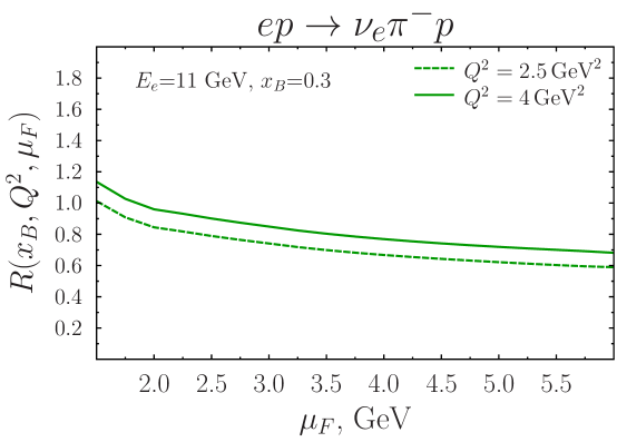
Figure 4: (color online) Factorization scale dependence of the charged current process $ep\to\nu_{e}\pi^{-}p$. The ratio $R$ is defined as $R\left(x_{B},\,Q^{2},\,\mu_{F}\right)=d\sigma\left(x_{B},\,Q^{2},\,\mu_{F}\right)/d\sigma\left(x_{B},\,Q^{2},\,\mu_{F}=Q\right)$. A similar dependence is observed for all other processes.

In Figure 5 we show the predictions for the differential cross-section $d\sigma/dx_{B}\,dQ^{2}$ for charged pion production for two virtualities $Q^{2}$. At fixed electron energy $E_{e}$ and virtuality $Q^{2}$, the cross-section as a function of $x_{B}$ has a a similar bump-like shape, which is explained by an interplay of two factors. For small $x_{B}\sim Q^{2}/2m_{N}E_{e}$ the elasticity $y$ defined in (3) approaches one, which causes a suppression due to a prefactor in (1). In the opposite limit, the suppression $\sim(1-x)^{n}$ is due to the implemented parametrization of GPDs. Since the contribution of NLO terms is sizable, for its evaluation we use coefficient functions which account for NLO corrections. To estimate the uncertainty due to higher order corrections (represented by the green band), we varied the factorization scale $\mu_{F}$ in the range $\mu_{F}\in\left(Q/2,\,2Q\right)$. As was discussed in Section II, the coefficient functions (14,II,II) have nonanalytic behavior $\sim\ln^{2}v$ in the region of small-$v,\bar{v}=(\xi\pm x)/2\xi$, and therefore this region requires special attention. Physically, collinear factorization is not valid here and the transverse momenta of mesons become important. In order to assess the relative contribution of this region, we performed an evaluation with NLO corrections switched off in the range $|v|\lesssim l_{\pi,\perp}^{2}/Q^{2}$, where the average transverse momentum of the pion $l_{\pi,\perp}\approx 0.3-0.4\,{\rm GeV}$ was estimated from the pion charge form factor Amendolia:1984nz ; Dally:1982zk ; Schlumpf:1994bc . As we can see from a comparison of solid and dashed lines, the contribution of the small-$|v|$ region is quite small, and therefore we expect that collinear factorization should give a reliable estimate in the considered kinematics. In the rightmost pane of the Figure 5, we have shown the relative (dominant) contribution of the GPDs $H^{u},H^{d}$ to the total result. Contributions of helicity flip and gluon GPDs constitute a minor ($\sim$10%) correction to the full cross-section.

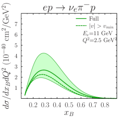
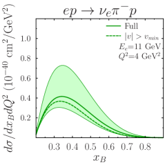
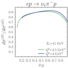
Figure 5: (color online) Left and central plots: Charged current pion production cross-section on a proton target at fixed electron energy, for virtualities $Q^{2}$=2.5 GeV²(left) and $Q^{2}$=4 GeV²(center) . Evaluations are performed using NLO coefficient functions, as discussed in Section II. The width of the band represents the uncertainty due to the factorization scale choice $\mu_{F}\in\left(Q/2,\,2Q\right)$, as explained in the text. The dashed line corresponds to evaluation with omitted NLO corrections in the region of $x\approx\pm\xi$, where collinear factorization might give sizable corrections $\sim\mathcal{O}\left(l_{\perp}^{2}/Q^{2}\right)$. Right plot: Relative contribution of GPDs $H^{u},H^{d}$ to the total result.

The contribution of the asymptotic Bethe-Heitler mechanism introduced in Section III is shown in the left pane of the Figure 6. We can see that for 11 GeV electron beams, its contribution is small and does not exceed $\sim 1\,$ per cent. The smallness of the harmonics $c_{n},\,s_{n}$ is explained by the fact that the kinematic prefactor $\sim\left(Q^{2}/t\right)$ enhancement in JLAB kinematics is not sufficient to compensate the suppression $\sim\mathcal{O}\left(\alpha_{{\rm em}}\right)$. Though formally both the BH term (23) and interference term (29) lead to appearance of the harmonics $c_{0},...,c_{2}$, the contribution from the former is suppressed by an additional power of $\alpha_{{\rm em}}$ and thus in JLAB kinematics the harmonics get a major contribution from the interference term. For the same reason, the harmonics $c_{2}$ (not shown in the plot) is extremely small: it gets contribution only from BH. In the right pane of the plot we have shown similar harmonics generated due to twist-three interference. The largest harmonics $c_{1}$ does not exceed 20 per cent and after averaging over the angle $\varphi$ does not contribute to the total cross-section $d\sigma/dx_{B}dQ^{2}$. The harmonics $c_{0}$, which contributes to the integrated cross-section $d\sigma/dx_{B}dQ^{2}$ as a multiplicative factor $1+c_{0}$, in the region of interest ($x_{B}\approx 0.4\pm 0.2$) is small and constitutes a few percent correction.

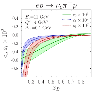
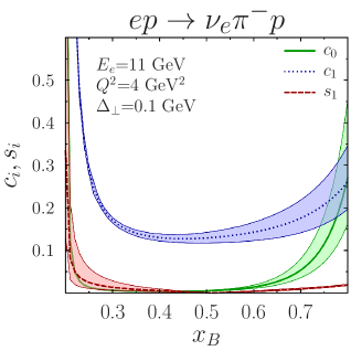
Figure 6: (color online) Left: Harmonics $c_{n},\,s_{n}$ in charged current pion production on a proton target, due to the interference with the Bethe-Heitler contribution. Right: Harmonics $c_{n},\,s_{n}$ generated due to twist-2 and twist-3 GPDs interference. In both plots the evaluations are performed using NLO coefficient functions, as discussed in Section II. The width of the band represents the uncertainty due to the factorization scale choice $\mu_{F}\in\left(Q/2,\,2Q\right)$, as explained in the text.

For deeply virtual meson production in other channels the cross-section gets comparable contributions from GPDs of different partons. For this reason restrictions imposed by experimental data on GPDs of individual partons are less binding. Additionally, these channels present more challenges for experimental study. For example, for charged current kaon production (see left pane in the Figure 7), we observe that the cross-section is small due to Cabibbo suppression ($\Delta S=1$), so the statistical error will be larger. From the central pane in the Figure 7 we can see that the total cross-section of this process gets a sizable contribution from quark-gluon interference. Similarly, for charged current pion production on a neutron (right pane in the Figure 7), the cross-section gets significant contributions from gluon GPDs and its interference with quarks, and experimentally the precision will be affected by uncertainty in the reconstruction of scattered neutron kinematics.

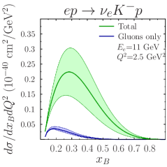
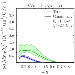
Figure 7: (color online) Left: Charged current kaon production cross-sections for fixed energy electron beam ($E_{e}\approx 11$ GeV). Central: relative fractions of different GPD components to the kaon production cross-section. We can see that the interference between quark and gluons is large and contributes with a negative sign. Right: Charged current pion production on a neutron target. In all plots the evaluations are performed using NLO coefficient functions, as discussed in Section II. The width of the band represents the uncertainty due to the factorization scale choice $\mu_{F}\in\left(Q/2,\,2Q\right)$, as explained in the text.

For this reason we believe that the study of the GPDs with charged currents should be focused on the $ep\to\nu_{e}\pi^{-}p$ channel.

VI Conclusions

In this paper we have shown that generalized parton distributions can be probed in charged current meson production processes, $ep\to\nu_{e}\pi^{-}p$. In contrast to pion photoproduction, these processes get a major contribution from the unpolarized GPDs $H^{u},\,H^{d}$, and thus could be used to supplement studies of these GPDs in DVCS. The undetectability of the produced neutrino will not present major challenges for the kinematics reconstruction, since all final state hadrons are charged. We estimated the cross-sections in the kinematics of the upgraded 12 GeV Jefferson Laboratory experiments and found that thanks to the large luminosity, the process can be measured with reasonable statistics. We also estimated the contaminating contributions from the Bethe-Heitler mechanism and twist-three corrections due to transversity GPDs. We found that both are small, and for this reason the $ep\to\nu_{e}\pi^{-}p$ channel presents a clean probe of the target GPDs . If polarized targets become available in these experiments, it could enable to study various beam-target asymmetries, sensitive to the smaller GPDs $E,\,\tilde{H},\,\tilde{E}$.

A code for the evaluation of the cross-sections, with various GPD models, is available on demand.

References

- (1) X. D. Ji and J. Osborne, Phys. Rev. D 58 (1998) 094018 [arXiv:hep-ph/9801260].
- (2) J. C. Collins and A. Freund, Phys. Rev. D 59, 074009 (1999).
- (3) R. Duprᅵ, M. Guidal, S. Niccolai and M. Vanderhaeghen, arXiv:1704.07330 [hep-ph].
- (4) D. Mueller, D. Robaschik, B. Geyer, F. M. Dittes and J. Horejsi, Fortsch. Phys. 42, 101 (1994) [arXiv:hep-ph/9812448].
- (5) X. D. Ji, Phys. Rev. D 55, 7114 (1997).
- (6) X. D. Ji, J. Phys. G 24, 1181 (1998) [arXiv:hep-ph/9807358].
- (7) A. V. Radyushkin, Phys. Lett. B 380, 417 (1996) [arXiv:hep-ph/9604317].
- (8) A. V. Radyushkin, Phys. Rev. D 56, 5524 (1997).
- (9) A. V. Radyushkin, arXiv:hep-ph/0101225.
- (10) J. C. Collins, L. Frankfurt and M. Strikman, Phys. Rev. D 56, 2982 (1997).
- (11) S. J. Brodsky, L. Frankfurt, J. F. Gunion, A. H. Mueller and M. Strikman, Phys. Rev. D 50, 3134 (1994).
- (12) K. Goeke, M. V. Polyakov and M. Vanderhaeghen, Prog. Part. Nucl. Phys. 47, 401 (2001) [arXiv:hep-ph/0106012].
- (13) M. Diehl, T. Feldmann, R. Jakob and P. Kroll, Nucl. Phys. B 596, 33 (2001) [Erratum-ibid. B 605, 647 (2001)] [arXiv:hep-ph/0009255].
- (14) A. V. Belitsky, D. Mueller and A. Kirchner, Nucl. Phys. B 629, 323 (2002) [arXiv:hep-ph/0112108].
- (15) M. Diehl, Phys. Rept. 388, 41 (2003) [arXiv:hep-ph/0307382].
- (16) A. V. Belitsky and A. V. Radyushkin, Phys. Rept. 418, 1 (2005) [arXiv:hep-ph/0504030].
- (17) V. Kubarovsky [CLAS Collaboration], Nucl. Phys. Proc. Suppl. 219-220, 118 (2011).
- (18) S. Ahmad, G. R. Goldstein and S. Liuti, Phys. Rev. D 79 (2009) 054014 [arXiv:0805.3568 [hep-ph]].
- (19) S. V. Goloskokov and P. Kroll, Eur. Phys. J. C 65, 137 (2010) [arXiv:0906.0460 [hep-ph]].
- (20) S. V. Goloskokov and P. Kroll, Eur. Phys. J. A 47, 112 (2011) [arXiv:1106.4897 [hep-ph]].
- (21) G. R. Goldstein, J. O. G. Hernandez and S. Liuti, arXiv:1201.6088 [hep-ph].
- (22) I. V. Anikin, D. Y. Ivanov, B. Pire, L. Szymanowski and S. Wallon, Nucl. Phys. B 828, 1 (2010) [arXiv:0909.4090 [hep-ph]].
- (23) M. Diehl, T. Gousset and B. Pire, Phys. Rev. D 59, 034023 (1999) [hep-ph/9808479].
- (24) L. Mankiewicz, G. Piller and A. Radyushkin, 10, 307 (1999) [hep-ph/9812467].
- (25) L. Mankiewicz and G. Piller, Phys. Rev. D 61, 074013 (2000) [hep-ph/9905287].
- (26) R. Boussarie, B. Pire, L. Szymanowski and S. Wallon, arXiv:1708.09164 [hep-ph].
- (27) E. R. Berger, M. Diehl and B. Pire, Eur. Phys. J. C 23, 675 (2002) [hep-ph/0110062].
- (28) B. Pire, L. Szymanowski and J. Wagner, Phys. Rev. D 79, 014010 (2009) [arXiv:0811.0321 [hep-ph]].
- (29) M. Boï¿œr, M. Guidal and M. Vanderhaeghen, Eur. Phys. J. A 51, no. 8, 103 (2015).
- (30) D. Mueller, B. Pire, L. Szymanowski and J. Wagner, Phys. Rev. D 86, 031502 (2012) [arXiv:1203.4392 [hep-ph]].
- (31) T. Sawada, W. C. Chang, S. Kumano, J. C. Peng, S. Sawada and K. Tanaka, Phys. Rev. D 93, no. 11, 114034 (2016) [arXiv:1605.00364 [nucl-ex]].
- (32) D. Y. Ivanov, A. Schafer, L. Szymanowski and G. Krasnikov, Eur. Phys. J. C 34, no. 3, 297 (2004) Erratum: [Eur. Phys. J. C 75, no. 2, 75 (2015)] [hep-ph/0401131].
- (33) D. Y. Ivanov, B. Pire, L. Szymanowski and J. Wagner, arXiv:1510.06710 [hep-ph].
- (34) F. Gautheron et al. [COMPASS Collaboration], SPSC-P-340, CERN-SPSC-2010-014.
- (35) O. Kouznetsov [COMPASS Collaboration], Nucl. Part. Phys. Proc. 270-272, 36 (2016).
- (36) A. Ferrero [COMPASS Collaboration], AIP Conf. Proc. 1523, 75 (2012).
- (37) A. Sandacz [COMPASS Collaboration], J. Phys. Conf. Ser. 678, no. 1, 012045 (2016).
- (38) A. Sandacz [COMPASS Collaboration], PoS QCDEV 2016, 018 (2017).
- (39) L. Silva, Few Body Syst. 54, no. 7-10, 1075 (2013).
- (40) P. Kroll, JPS Conf. Proc. 13, 010014 (2017).
- (41) B. Z. Kopeliovich, I. Schmidt and M. Siddikov, Phys. Rev. D 86 (2012), 113018 [arXiv:1210.4825 [hep-ph]].
- (42) D. Drakoulakos et al. [Minerva Collaboration], hep-ex/0405002.
- (43) B. Z. Kopeliovich, I. Schmidt and M. Siddikov, Phys. Rev. D 89, no. 5, 053001 (2014) [arXiv:1401.1547 [hep-ph]].
- (44) M. Siddikov and I. Schmidt, Phys. Rev. D 95, no. 1, 013004 (2017) [arXiv:1611.07294 [hep-ph]].
- (45) L. L. Frankfurt, P. V. Pobylitsa, M. V. Polyakov and M. Strikman, Phys. Rev. D 60 (1999) 014010 [hep-ph/9901429].
- (46) B. Pire and L. Szymanowski, Phys. Rev. Lett. 115 (2015), 092001 [arXiv:1505.00917 [hep-ph]].
- (47) B. Pire and L. Szymanowski, Acta Phys. Polon. Supp. 8, 883 (2015) [arXiv:1510.01869 [hep-ph]].
- (48) B. Pire, L. Szymanowski and J. Wagner, EPJ Web Conf. 112, 01018 (2016) [arXiv:1601.07666 [hep-ph]].
- (49) B. Pire, L. Szymanowski and J. Wagner, Phys. Rev. D 95, no. 9, 094001 (2017) [arXiv:1702.00316 [hep-ph]].
- (50) B. Pire, L. Szymanowski and J. Wagner, Phys. Rev. D 95, no. 11, 114029 (2017) [arXiv:1705.11088 [hep-ph]].
- (51) D. Androic et al. [Qweak Collaboration], Phys. Rev. Lett. 111 (2013) no.14, 141803 [arXiv:1307.5275 [nucl-ex]].
- (52) J. Alcorn et al., Nucl. Instrum. Meth. A 522, 294 (2004).
- (53) M. Vanderhaeghen, P. A. M. Guichon and M. Guidal, Phys. Rev. Lett. 80, 5064 (1998).
- (54) S. V. Goloskokov and P. Kroll, Eur. Phys. J. C 50, 829 (2007) [hep-ph/0611290].
- (55) S. V. Goloskokov and P. Kroll, Eur. Phys. J. C 53, 367 (2008) [arXiv:0708.3569 [hep-ph]].
- (56) S. V. Goloskokov and P. Kroll, Eur. Phys. J. C 59 (2009) 809 [arXiv:0809.4126 [hep-ph]].
- (57) B. Z. Kopeliovich, Ivï¿œn Schmidt and M. Siddikov, Nucl. Phys. A 918, 41 (2013) [arXiv:1108.5654 [hep-ph]].
- (58) A. V. Belitsky and D. Mueller, Phys. Lett. B 513, 349 (2001) [hep-ph/0105046].
- (59) D. Y. Ivanov, L. Szymanowski and G. Krasnikov, JETP Lett. 80, 226 (2004) [Pisma Zh. Eksp. Teor. Fiz. 80, 255 (2004)] Erratum: [JETP Lett. 101, no. 12, 844 (2015)] , [hep-ph/0407207].
- (60) M. Diehl and W. Kugler, Eur. Phys. J. C 52, 933 (2007) [arXiv:0708.1121 [hep-ph]].
- (61) E. Braaten and S. M. Tse, Phys. Rev. D 35, 2255 (1987).
- (62) B. Melic, B. Nizic and K.~Passek, Phys. Rev. 60, 074004 (1999) [hep-ph/9802204].
- (63) B. Z. Kopeliovich, I. Schmidt and M. Siddikov, Phys. Rev. D 87, 033008 (2013) [arXiv:1301.7014 [hep-ph]].
- (64) S. R. Amendolia et al., Phys. Lett. 146B (1984) 116.
- (65) E. B. Dally et al., Phys. Rev. Lett. 48, 375 (1982).
- (66) F. Schlumpf, Phys. Rev. D 50, 6895 (1994) [hep-ph/9406267].