Estimating phylogenetic distances between genomic sequences based on the length distribution of $k$-mismatch common substrings

Abstract

Various approaches to alignment-free sequence comparison are based on the length of exact or inexact word matches between two input sequences. Haubold et al. (2009) showed how the average number of substitutions between two DNA sequences can be estimated based on the average length of exact common substrings. In this paper, we study the length distribution of $k$-mismatch common substrings between two sequences. We show that the number of substitutions per position that have occurred since two sequences have evolved from their last common ancestor, can be estimated from the position of a local maximum in the length distribution of their $k$-mismatch common substrings.

1 Introduction

Phylogenetic distances between DNA or protein sequences are usually estimated based on pairwise or multiple sequence alignments. Since sequence alignment is computationally expensive, alignment-free phylogeny approaches have become popular in recent years, see Vinga [33] for a review. Some of these approaches compare the word composition [13, 28, 4, 34] or spaced-word composition [16, 21, 8, 22] of sequences using a fixed word length or pattern of match and don’t-care positions, respectively. Other approaches are based on the matching statistics [3], that is on the length of common substrings of the input sequences [32, 5]. All these methods are much faster than traditional alignment-based approaches. A disadvantage of most word-based approaches to phylogeny reconstruction is that they are not based on explicit models of molecular evolution. Instead of estimating distances in a statistically rigorous sense, they only return rough measures of sequence similarity or dissimilarity.

The average common substring (ACS) approach [32] calculates for each position in one sequence the length of the longest substring starting at this position that matches a substring of the other sequence. The average length of these substring matches is then used to quantify the similarity between two sequences based on information-theoretical considerations; these similarity values are finally transformed into symmetric distance values. More recently, we generalized the ACS approach by considering common substrings with up to $k$ mismatches instead of exact substring matches [18]. To calculate distance values between two sequences from the average length of $k$-mismatch common substrings, we used the same information-theoretical approach as in ACS. Since there is no exact solution to the $k$-mismatch longest common substring problem that is fast enough to be applied to long genomic sequences, we proposed a simple heuristic: we first search for longest common exact matches and then extend these matches until the $k+1$st mismatch occurs. Distances are then calculated from the average length of these $k$-mismatch common substrings similarly as in ACS; the implementation of this approach is called kmacs.

Various algorithms have been proposed in recent years to calculate exact or approximate solutions for the $k$-mismatch average common substring problem as a basis for phylogeny reconstruction [1, 30, 24, 29, 2, 24, 31, 23]. Like ACS and kmacs, these approaches do not estimate the ‘real’ pairwise distances between sequences in terms of substitutions per position. Instead, they calculate various sorts of distance measures that vaguely reflect evolutionary distances.

To our knowledge, the first alignment-free approach to estimate the phylogenetic distance between two DNA sequences in a statistically rigorous way was the program kr by Haubold et al. [10]. These authors showed that the average number of nucleotide substitutions per position between two DNA sequences can be estimated by calculating for each position $i$ in the first sequence the length of the shortest substring starting at $i$ that does not occur in the second sequence, see also [11, 12]. This way, phylogenetic distances between DNA sequences can be accurately estimated for distances up to around $0.5$ substitutions per position. Some other, more recent alignment-free approaches also estimate phylogenetic distances based on a stochastic model of molecular evolution, namely Co-phylog [35], andi [9], an approach based on the number of (spaced-) word matches [21] and Filtered Spaced Word Matches [17].

In this paper, we propose a new approach to estimate phylogenetic distances based on the length distribution of $k$-mismatch common substrings. The manuscript is organized as follows. In section 2, we introduce some notation and the stochastic model of sequence evolution that we are using. In section 3, we recapitulate a result from [10] on the length distribution of longest common substrings, which we generalize in section 4 to $k$-mismatch longest common substrings, and in section 5, we study the length distribution of $k$-mismatch common substrings returned by the kmacs heuristic [18]. In sections 6 and 7, we introduce our new approach to estimate phylogenetic distances and explain some implementation details. Finally, sections 8 and 9 report on benchmarking results, discusses these results and address some possible future developments.

We should mention that sections 4 and 5 are not necessary to understand our novel approach to distance estimation, except for equation (3) which gives the length distribution of $k$-mismatch common substrings at given positions $i$ and $j$. We added these two sections for completeness, and since the results could be the basis for alternative ways to estimate phylogenetic distances. But readers who are mainly interested in our approach to distance estimation can skip sections 4 and 5.

2 Sequence model and notation

We use standard notation such as used in [7]. For a sequence $S$ of length $L$ over some alphabet, $S(i)$ is the $i$-th character in $S$. $S[i..j]$ denotes the (contiguous) substring from $i$ to $j$; we say that $S[i..j]$ is a substring at $i$. In the following, we consider two DNA sequences $S_{1}$ and $S_{2}$ that are assumed to have descended from an unknown common ancestor under the Jukes-Cantor model [14]. That is, we assume that substitutions at different positions are independent of each other, that we have a constant substitution rate at all positions and that all substitutions occur with the same probability. Thus, we have $p$ and $q$ with

$$P\left(S_{1}(i)=S_{2}(j)\right)=\left\{\begin{array}[]{ll}p&\text{ if }i=j\\ q&\text{ else }\\ \end{array}\right.$$

Moreover, we use a gap-free model of evolution to simplify the considerations below. Note that, with a gap-free model, it is trivial to estimate the number of substitutions since two sequences diverged from their last common ancestor, simply by counting the number of mismatches in the gap-free alignment and then applying the usual Jukes-Cantor correction. However, we will to apply this simple model to real-world sequences with insertions and deletions where this trivial approach is not possible.

3 Average common substring length

For positions $i$ and $j$ in sequence $S_{1}$ and $S_{2}$, respectively, we define random variables

$$X_{i,j}=\max\{l:X[i..i+l-1]=X[j..j+l-1]\}$$

as the length of the longest substring at $i$ that exactly matches a substring at $j$. Next, we define

$$X_{i}=\max_{1\leq j\leq L}X_{i,j}$$

as the length of the longest substring at $i$ that matches a substring of $S_{2}$.

In the following, we ignore edge effects which is justified if long sequences are compared since the probability of $k$-mismatch common substrings of length $m$ decreases rapidly if $m$ increases. With this simplification, we have

$$P(X_{i,j}<n)=1-P(X_{i,j}\geq n)=\left\{\begin{array}[]{ll}1-p^{n}&\text{ if }i=j\\ 1-q^{n}&\text{ else }\\ \end{array}\right.$$

If, in addition, we assume equilibrium frequencies for the nucleotides, i.e. if we assume that each nucleotide occurs at each sequence position with probability $0.25$, the random variables $X_{i,j}$ and $X_{i^{\prime},j^{\prime}}$ are independent of each other whenever $j-i\not=j^{\prime}-i^{\prime}$ holds. In this case, we have for $n\leq L-i+1$

$${P(X_{i}<n)=P(X_{i,1}<n\wedge\ldots\wedge X_{i,L}<n)}$$ (1)

$$=P(X_{i,1}<n)\cdot\ldots\cdot P(X_{i,L}<n)$$

$$=(1-q^{n})^{L-1}\cdot(1-p^{n})$$

and

$${P(X_{i}=n)=P(X_{i}<n+1)-P(X_{i}<n)}$$

$$=(1-q^{n+1})^{L-1}\cdot(1-p^{n+1})-(1-q^{n})^{L-1}\cdot(1-p^{n})$$

so the expected length of the longest common substring at a given sequence position is

$$E(X)=\sum_{n=1}^{L}n\cdot\left((1-q^{n+1})^{L-1}\cdot(1-p^{n+1})-(1-q^{n})^{L-1}\cdot(1-p^{n})\right)$$ (2)

4 $k$-mismatch average common substring length

Next, we generalize the above considerations by considering the average length of the $k$-mismatch longest common substrings between two sequences for some integer $k\geq 0$. That is, for a position $i$ in one of the sequences, we consider the longest substring starting at $i$ that matches some substring in the other sequence with a Hamming distance $\leq k$. Generalizing the above notation, we define random variables

$$X_{i,j}^{(k)}=\max\left\{l:d_{H}\left(S_{1}[i..i+l-1],S_{2}[j..j+l-1]\right)\leq k\right\}$$

where $d_{H}(\cdot,\cdot)$ is the Hamming distance between two sequences. In other words, $X_{i,j}^{(k)}$ is the length of the longest substring starting at position $i$ in sequence $S_{1}$ that matches a substring starting at position $j$ in sequence $S_{2}$ with to $k$ mismatches. Accordingly, we define

$$X_{i}^{(k)}=\max_{j}X^{(k)}_{i,j}$$

as the length of the longest $k$-mismatch substring at position $i$. As pointed out by Apostolico et al. [2], $X^{(k)}_{i,j}$ follows a negative binomial distribution. More precisely, we have $X^{(k)}_{i,j}\sim NB(n-k;k-1,p)$, and we can write

$$P\left(X^{(k)}_{i,j}=n\right)=\left\{\begin{array}[]{ll}{n\choose k}p^{n-k}(1-p)^{k+1}&\text{ if }i=j\\ {n\choose k}q^{n-k}(1-q)^{k+1}&\text{ else }\\ \end{array}\right.$$ (3)

and

$$P\left(X^{(k)}_{i,j}\geq n\right)=\left\{\begin{array}[]{ll}\sum_{k^{\prime}\leq k}{n\choose k^{\prime}}p^{n-k^{\prime}}(1-p)^{k^{\prime}}&\text{ if }i=j\\ \sum_{k^{\prime}\leq k}{n\choose k^{\prime}}q^{n-k^{\prime}}(1-q)^{k^{\prime}}&\text{ else }\\ \end{array}\right.$$ (4)

Generalizing (1), we obtain for $n>k$

$$P\left(X_{i}^{(k)}<n\right)=$$

$$\left(1-\sum_{k^{\prime}\leq k}{n\choose k^{\prime}}q^{n-k^{\prime}}(1-q)^{k^{\prime}}\right)^{L+i-1}\cdot\left(1-\sum_{k^{\prime}\leq k}{n\choose k^{\prime}}p^{n-k^{\prime}}(1-p)^{k^{\prime}}\right)$$

while we have

$$P\left(X_{i}^{(k)}<n\right)=\left\{\begin{array}[]{ll}1&\text{ if }n>L-i+1\\ 0&\text{ if }n\leq k\\ \end{array}\right.$$

Finally, we obtain

$$P\left(X_{i}^{(k)}=n\right)=\left.\left(1-\sum_{k^{\prime}\leq k}{n+1\choose k^{\prime}}q^{n+1-k^{\prime}}(1-q)^{k^{\prime}}\right)^{L+i-1}\right.$$

$$\cdot\left(1-\sum_{k^{\prime}\leq k}{n+1\choose k^{\prime}}p^{n+1-k^{\prime}}(1-p)^{k^{\prime}}\right)$$

$$- \left.\left(1-\sum_{k^{\prime}\leq k}{n\choose k^{\prime}}q^{n-k^{\prime}}(1-q)^{k^{\prime}}\right)^{L+i-1}\cdot\left(1-\sum_{k^{\prime}\leq k}{n\choose k^{\prime}}p^{n-k^{\prime}}(1-p)^{k^{\prime}}\right)\right.$$

from which one can obtain the expected length of the $k$-mismatch longest substrings.

5 Heuristic used in kmacs

Since exact solutions for the average $k$-mismatch common substring problem are too time-consuming for large sequence sets, the program kmacs [18] uses a heuristic. In a first step, the program calculates for each position $i$ in one sequence, the length of the longest substring starting at $i$ that exactly matches a substring of the other sequence. kmacs then calculates the length of the longest gap-free extension of this exact match with up to $k$ mismatches. Using standard indexing structures, this can be done in $O(L\cdot k)$ time.

For sequences $S_{1},S_{2}$ as above and a position $i$ in $S_{1}$, let $j^{*}$ be a position in $S_{2}$ such that the $X_{i}$-length substring starting at $i$ matches the $X_{i}$-length substring at $j^{*}$ in $S_{2}$. That is, the substring

$$S_{2}[j^{*}..j^{*}+X_{i}-1]$$

is the longest substring of $S_{2}$ that matches a substring of $S_{1}$ at position $i$. In case there are several such positions in $S_{2}$, we assume for simplicity that $j^{*}\not=i$ holds (in the following, we only need to distinguish the cases $j^{*}=i$ and $j^{*}\not=i$, otherwise it does not matter how $j^{*}$ is chosen). Now, let the random variable $\tilde{X}^{(k)}_{i}$ be defined as the length of the $k$-mismatch common substring starting at $i$ and $j^{*}$, so we have

$$\tilde{X}^{(k)}_{i}=X_{i,j^{*}}^{(k)}=X_{i}+X^{(k-1)}_{i+X_{i},j^{*}+X_{i}}+1$$ (7)

Theorem 5.1.

For a pair of sequences as above, $1\leq i\leq L$ and $m\leq L+i$, the probability of the heuristic kmacs hit of having a length of $m$ is given as

$${P\left(\tilde{X}^{(k)}_{i}=m\right)}$$

$$= \ \ p^{m-k+1}(1-p)^{k+1}\sum_{m_{1}+m_{2}=m}(1-q^{m_{1}+1})^{L-1}{m_{2}\choose k-1}$$

$$+\sum_{m_{1}+m_{2}=m}\left[(1-q^{m_{1}+1})^{L-1}-(1-q^{m_{1}})^{L-1}\right]\cdot(1-p^{m_{1}})$$

$$\ \ {m_{2}\choose k-1}q^{m_{2}-k+1}(1-q)^{k}$$

Proof.

Distinguishing between ‘homologous’ and ‘background’ matches, we can write

$${P\left(\tilde{X}^{(k)}_{i}=m\right)}=P\left(\tilde{X}^{(k)}_{i}=m\middle|j^{*}=i\right)P(j^{*}=i)$$ (8)

$$+ P\left(\tilde{X}^{(k)}_{i}=m\middle|j^{*}\not=i\right)P(j^{*}\not=i)$$

and with (3), we obtain

$$P\left(\tilde{X}^{(k)}_{i}=m\middle|j^{*}=i\right)$$ (9)

$$=\sum_{m_{1}+m_{2}=m}P(X_{i}=m_{1}|j^{*}=i)P\left(X_{i+m_{1},i+m_{1}}^{(k-1)}=m_{2}\right)$$

$$=\sum_{m_{1}+m_{2}=m}P(X_{i}=m_{1}|j^{*}=i){m_{2}\choose k-1}p^{m_{2}-k+1}(1-p)^{k}$$

and

$$P(X_{i}=m_{1}|j^{*}=i)=\frac{P(X_{i,i}=m_{1}\wedge j^{*}=i)}{P(j^{*}=i)}$$ (10)

$$=\frac{P(X_{i,i}=m_{1}\wedge X_{i,i}\geq X_{i,j},j\not=i)}{P(j^{*}=i)}$$

$$=\frac{P(X_{i,i}=m_{1}\wedge X_{i,j}\leq m_{1},j\not=i)}{P(j^{*}=i)}$$

$$=\frac{p^{m_{1}}(1-p)\cdot(1-q^{m_{1}+1})^{L-1}}{P(j^{*}=i)}$$

so with (9) and (10), the first summand in (8) becomes

$$P\left(\tilde{X}^{(k)}_{i}=m\middle|j^{*}=i\right)P(j^{*}=i)$$ (11)

$$= \sum_{m_{1}+m_{2}=m}P(X_{i}=m_{1}|j^{*}=i){m_{2}\choose k-1}p^{m_{2}-k+1}(1-p)^{k}\cdot P(j^{*}=i)$$

$$= \sum_{m_{1}+m_{2}=m}\frac{p^{m_{1}}(1-p)\cdot(1-q^{m_{1}+1})^{L-1}}{P(j^{*}=i)}$$

$$\ \ {m_{2}\choose k-1}p^{m_{2}-k+1}(1-p)^{k}\cdot P(j^{*}=i)$$

$$= \sum_{m_{1}+m_{2}=m}(1-q^{m_{1}+1})^{L-1}{m_{2}\choose k-1}p^{m_{1}+m_{2}-k+1}(1-p)^{k+1}$$

$$= \ \ p^{m-k+1}(1-p)^{k+1}\sum_{m_{1}+m_{2}=m}(1-q^{m_{1}+1})^{L-1}{m_{2}\choose k-1}$$

Similarly, for the second summand in (8), we note that

$$P\left(\tilde{X}^{(k)}_{i}=m\middle|j^{*}\not=i\right)$$ (12)

$$=\sum_{m_{1}+m_{2}=m}P(X_{i}=m_{1}|j^{*}\not=i){m_{2}\choose k-1}q^{m_{2}-k+1}(1-q)^{k}$$

and

$$P(X_{i}=m_{1}|j^{*}\not=i)=\frac{P(X_{i,j^{*}}=m_{1}\wedge j^{*}\not=i)}{P(j^{*}\not=i)}$$ (13)

$$=\frac{P(X_{i,j^{*}}=m_{1}\wedge X_{i,i}<X_{i,j^{*}})}{P(j^{*}\not=i)}$$

$$=\frac{P(X_{i,j^{*}}=m_{1}\wedge X_{i,i}<m_{1})}{P(j^{*}\not=i)}$$

$$=\frac{P(\max_{j\not=i}X_{i,j}=m_{1}\wedge X_{i,i}<m_{1})}{P(j^{*}\not=i)}$$

$$=\frac{P(\max_{j\not=i}X_{i,j}=m_{1})\cdot P(X_{i,i}<m_{1})}{P(j^{*}\not=i)}$$

$$=\frac{P(\max_{j\not=i}X_{i,j}=m_{1})\cdot P(X_{i,i}<m_{1})}{P(j^{*}\not=i)}$$

$$=\frac{\left[(1-q^{m_{1}+1})^{L-1}-(1-q^{m_{1}})^{L-1}\right]\cdot(1-p^{m_{1}})}{P(j^{*}\not=i)}$$

Thus, the second summand in (8) is given as

$${P\left(\tilde{X}^{(k)}_{i}=m\middle|j^{*}\not=i\right)P(j^{*}\not=i)}$$

$$= \sum_{m_{1}+m_{2}=m}P(X_{i}=m_{1}|j^{*}\not=i){m_{2}\choose k-1}q^{m_{2}-k+1}(1-q)^{k}\cdot P(j^{*}\not=i)$$

$$= \sum_{m_{1}+m_{2}=m}\frac{\left[(1-q^{m_{1}+1})^{L-1}-(1-q^{m_{1}})^{L-1}\right]\cdot(1-p^{m_{1}})}{P(j^{*}\not=i)}$$

$$\ \ {m_{2}\choose k-1}q^{m_{2}-k+1}(1-q)^{k}\cdot P(j^{*}\not=i)$$

$$= \sum_{m_{1}+m_{2}=m}\left[(1-q^{m_{1}+1})^{L-1}-(1-q^{m_{1}})^{L-1}\right]\cdot(1-p^{m_{1}})$$

$$\ \ {m_{2}\choose k-1}q^{m_{2}-k+1}(1-q)^{k}$$

∎

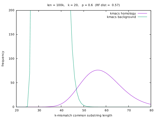
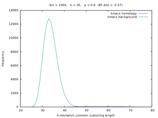
Figure 1: Length distribution of the background and homologous $k$-mismatch longest common substrings for a pair of DNA sequences under the Jukes-Cantor model. For each possible length, the expected number of $k$-mismatch longest common substrings of this length returned by the kmacs heuristic is calculated using theorem 5.1 for an indel-free pair of sequences of length $L=100kb$, a match probability $p=0.6$ (corresponding to 0.57 substitutions per position) and $k=20$.

For $1\leq m\leq L$, the expected number of $k$-mismatch common substrings of length $m$ returned by the kmacs heuristics is given as $L\cdot P\left(\tilde{X}^{(k)}_{i}=m\right)$ and can be calculated using theorem 5.1. In Figure 1, these values are plotted against $m$ for $L=100$ kb, $p=0.6$ and $k=20$.

6 Distance estimation

Using theorem 5.1, one could estimate the match probability $p$ – and thereby the average number of substitutions per position – from the empirical average length of the $k$-mismatch common substrings returned by kmacs in a moment-based approach, similar to the approach proposed in [10].

A problem with this moment-based approach is that, for realistic values of $L$ and $p$, one has $P(j^{*}=i)\ll P(j^{*}\not=i)$, so the above sum is heavily dominated by the ‘background’ part, i.e. by the second summand in (8). For the parameter values used in Figure 1, for example, only 1 percent of the matches returned by kmacs represent homologies while 99 percent are background noise. There are, in principle, two ways to circumvent this problem. First, one could try to separate homologous from background matches using a suitable threshold values, similarly as we have done it in our Filtered Spaced Word Matches approach [19]. But this is more difficult for $k$-mismatch common substrings, since there is much more overlap between homologous and background matches than for Spaced-Word matches, see Figure 1.

There is an alternative to this moment-based approach, however. As can be seen in Figure 1, the length distribution of the $k$-mismatch longest common substrings is bimodal, with a first peak in the distribution corresponding to the background matches and the second peak corresponding to the homologous matches. We show that the number of substitutions per positions can be easily estimated from the position of this second peak.

To simplify the following calculations, we ignore the longest exact match in equation (7), and consider only the length of the gap-free ‘extension’ of this match. To model the length of these $k$-mismatch extensions, we define define random variables

$$\hat{X}^{(k)}_{i}=\tilde{X}_{i}^{(k+1)}-X_{i}=X^{(k)}_{i+X_{i}+1,j^{*}+X_{i}+1}$$ (14)

In other words, for a position $i$ in sequence $S_{1}$, we are looking for the longest substring starting at $i$ that exactly matches a substring of $S_{2}$. If $j^{*}$ is the starting position of this substring of $S_{2}$, we define $\hat{X}^{(k)}_{i}$ as the length of the longest possible substring of $S_{1}$ starting at position $i+X_{i}+1$ that matches a substring of $S_{2}$ starting at position $j^{*}+X_{i}+1$ with a Hamming distance of up to $k$.

Theorem 6.1.

Let $\hat{X}^{(k)}_{i}$ be defined as in (14). Then $\hat{X}^{(k)}_{i}$ is the sum of two unimodal distributions, the a ‘homologous’ and a ‘background’ contribution, and the maximum of the ‘homologous’ contribution is reached at

$$m_{H}=\left\lceil\frac{k}{1-p}-1\right\rceil$$

and the maximum of the ‘background contribution’ is reached at

$$m_{B}=\left\lceil\frac{k}{1-q}-1\right\rceil$$

Proof.

As in (3), the distribution of $\hat{X}^{(k)}_{i}$ conditional on $j^{*}=i$ or $j^{*}\not=i$, respectively, can be easily calculated as

$$P\left(\hat{X}^{(k)}_{i}=m\middle|j^{*}=i\right)=P\left(X^{(k)}_{i+X_{i}+1,i+X_{i}+1}=m\right)={m\choose k}p^{m-k}(1-p)^{k+1}$$

and

$$P\left(\hat{X}^{(k)}_{i}=m\middle|j^{*}\not=i\right)={m\choose k}q^{m-k}(1-q)^{k+1}$$

so we have

$$P\left(\hat{X}^{(k)}_{i}=m\right) =P(j^{*}=i){m\choose k}p^{m-k}(1-p)^{k+1}$$ (15)

$$+P(j^{*}\not=i){m\choose k}q^{m-k}(1-q)^{k+1}$$

For the homologous part

$$H_{k}(m)={m\choose k}p^{m-k}(1-p)^{k+1}$$

we obtain the recursion

$$H_{k}(m+1)=P(j^{*}=i)\frac{(m+1)}{m+1-k}\cdot p\cdot H_{k}(m)$$

so we have $H_{k}(m)<H_{k}(m+1)$ if and only if

$$\frac{m+1-k}{m+1}<p$$ (16)

Similarly, the ‘background contribution’

$$B_{k}(m)=P(j^{*}\not=i){m\choose k}q^{m-k}(1-q)^{k+1}$$

is increasing until

$$\frac{m+1-k}{m+1}<q$$

holds, which concludes the proof of the theorem ∎

Theorem 6.1 gives us an easy way to estimate the match probability $p$: By inserting the second local maximum $m_{\max}$ of the empirical distribution of $\hat{X}_{i}$ into (16), we obtain

$$\hat{p}\approx\frac{m_{\max}+1-k}{m_{\max}+1}$$ (17)

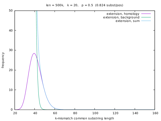
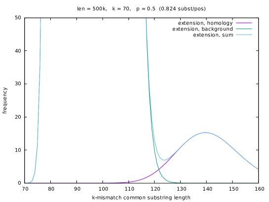
Figure 2: Detail of the expected length distributions of the $k$-mismatch extensions in kmacs for a pair of sequences of length $L=500$ kb with a match probability of $p=0.5$ for $k=10$ (top) and $k=70$ (bottom). Expected frequencies were calculated using equation (15), distinguishing between ‘homologous’ and ‘background’ matches. A large enough value of $k$ is necessary to detect the second peak in the distribution that corresponds to the ‘homologous’ matches.

Figure 3: Detail of the length distribution of the $k$-mismatch extensions in kmacs for a pair of simulated DNA sequences of length $L=500$ kb with $k=90$. (raw frequencies and smoothed distributions). Different parameters were used for for the width $w$ of the smoothing window. The hight of the ‘homologous’ peak is > 50,000

For completeness, we calculate the probability $P(j^{*}=i)$. First, we note that, for all $i$, we have

$$P\left(X_{i,j}<X_{i,i}\text{ for all }j\not=i\right)\leq P(j^{*}=i)\leq P(X_{i,j}\leq X_{i,i}\text{ for all }j\not=i)$$

and for all $m$ and $i\not=j$,

$$P(X_{i,j}<m)=1-q^{m}$$

and

$$P(X_{i,j}\leq m)=1-q^{m+1}$$

hold. Thus, we obtain

$${P\left(X_{i,j}<X_{i,i}\text{ for all }j\not=i\right)=\sum_{m}P\left(X_{i,j}<X_{i,i}\text{ for all }j\not=i|X_{i,i}=m\right)P(X_{i,i}=m)}$$ (18)

$$= \sum_{m}P\left(X_{i,j}<m\text{ for all }j\not=i\right)P(X_{i,i}=m)$$

$$= \sum_{m}\prod_{j\not=i}P(X_{i,j}<m)P(X_{i,i}=m)$$

$$=\sum_{m}(1-q^{m})^{L-1}p^{m}(1-p)$$

and similarly

$$P\left(X_{i,j}\leq X_{i,i}\text{ for all }j\not=i\right)=\sum_{m}(1-q^{m+1})^{L-1}p^{m}(1-p)$$ (19)

7 Implementation

For each position $i$ in one of two input sequences, kmacs first calculates the length of the longest substring starting at $i$ that exactly matches a substring of the other sequence. For a user-defined parameter $k$, the program then calculates the length of the longest possible gap-free extension with up to $k$ mismatches of this exact hit. The original version of the program uses the average length of these $k$-mismatch common substrings (the initial exact match plus the $k-1$-mismatch extension after the first mismatch) to calculate a distance between two sequences. We modified kmacs to output the length of the extensions of the identified exact matches. Thus, to find $k$-mismatch common substrings, we ran kmacs with parameter $k+1$, and we consider the length of the $k$-mismatch extension after the first mismatch. For each possible length $m$, the modified program outputs the number $N(m)$ of $k$-mismatch extensions of length $m$, starting after the first mismatch after the respective longest exact match.

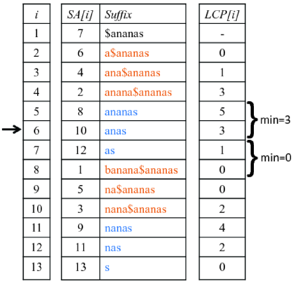
Figure 4: Enhanced suffix array for sequences banana and ananas. Suffixes of the concatenated sequence are lexicographically ordered; a longest common prefix (LCP) array indicates the length of the longest common prefix of a suffix with its predecessor in the list (Figure from [18]).

To find for each position $i$ in one sequence the length of the longest string at $i$ matching a substring of the other sequences, kmacs uses a standard procedure based on enhanced suffix arrays [20], see Figure 4. To find the longest exact match starting at $i$, the algorithm goes to the corresponding position in the suffix array. It then goes in both directions, up and down, in the suffix array until the first entry from the respective other sequence is found. In both cases, the minimum of the LCP values is recorded. The maximum of these two minima is the length of the longest substring in the other sequence matching a substring starting at $i$. In Figure 4, for example, if $i$ is position 3 in the string ananas, i.e. the 10th position in the concatenate string, the minimum LCP value until the first entry from banana is found, is 3 if one goes up the array and 0 if one goes down. Thus, the longest string in banana matching a substring starting at position 3 in ananas has length 3.

Note that, for a position $i$ in one sequence, it is possible that there exist more than one maximal substring in the other sequence matching a substring at $i$. In this case, our modified algorithm uses all of these maximal substring matches, i.e. all maximal exact string matches are extended as described above. All these hits can be easily found in the suffix array by extending the search in upwards or downwards direction until the minimum of the LCP entries decreases. In the above example, there is a second occurrence of ana in banana which is found by moving one more position upwards (the corresponding LCP value is still 3).

In addition, we modified the original kmacs to ensure that for each pair $(i,j)$ of positions from the two input sequences, only one single extended $k$-mismatch common substring is considered. The rationale behind this is as follows: if the two input sequences share a long common substring $S$, then there will be many positions $i$ in the first sequence within $S$ such that the longest exact string match at $i$ matches to a substring in $S$ in the second sequence. Thus, all these exact substring matches are identical up to different starting positions, so they end at the same first mismatch between $S_{1}$ and $S_{2}$. Consequently, the $k$-mismatch extensions of these exact matches are all exactly the same. As a result, for real-world sequences with long exact substrings, isolated positions $m$ in the length distribution of the $k$-mismatch common substrings can be observed with very large values $N(m)$ while $N(m^{\prime})=0$ for other values $m^{\prime}$ around $m$.

To further process the length distribution returned by the modified kmacs, we implemented a number of Perl scripts. First, the length distribution of the $k$-mismatch common substrings is smoothed using a window of length $w$. Next, we search for the second local maximum in this smoothed length distribution. This second peak should represent the homologous $k$-mismatch common substrings, while the first, larger peak represents the background matches, see Figures 3 and 2. A simple script identifies the position $m^{*}$ of the second highest local peak under two side constraints: we require the height $N(m^{*})$ of the second peak to be substantially smaller than the global maximum, and we required for that $N(m^{*})$ is larger than $N(m^{*}-x)$. Quite arbitrarily, we required the second peak to be 10 times smaller than the global maximum peak, and we used a value of $x=4$. These constraints were introduced to prevent the program to identify small side peaks within the background peak.

Finally, we use the position $m^{*}$ of the second largest peak in the smoothed length distribution of $k$-mismatch common substrings to estimate the match probability $p$ in an alignment of the two input sequences using expression (17). The usual Jukes-Cantor correction is then used to estimate the number of substitutions per position that have occurred since the two sequences separated from their last common ancestor.

We should mention that our algorithm is not always able to output a distance value for two input sequences. It is possible that the algorithm fails to find a second maximum in the length distribution of the $k$-mismatch common substrings, so in these cases no distance can be calculated.

8 Test Results

To evaluate our approach, we used simulated and real-world genome sequences. As a first set of test data, we generated pairs of simulated DNA sequences of length 500 kb with varying evolutionary distances and compared the distances estimated with our algorithm – i.e. the estimated number of substitutions per position – to their ‘real’ distances. For each distance value, we generated 100 pairs of sequences and calculated the average and standard deviation of the estimated distance values. Figure 5 shows the results of these test runs. with a parameter $k=90$ and a smoothing window size of $w=31$, with error bars representing standard deviations. A program run on a pair of sequences of length 500 kb took less than a second.

Figure 3 shows a detail of the length distribution for one of these sequence pairs with various values for $w$. In Figure 5, the results are reported for a given distance value, if distances could be computed for at least 75 out of the 100 sequence pairs. As can be seen in the figure, our approach accurately estimates evolutionary distances up to 0.9 around substitutions per position. For larger distances, the program did not return a sufficient number of distance values, so no results are reported here. To demonstrate the influence of the parameter $k$, we plotted in Figure 2, for a given set of parameters, the expected number of $k$-mismatch common substring extensions of length $m$, calculated with equation (15), against $m$.

As a real-word test case, we used a set of 27 mitochondrial genomes from primates that has been used as benchmark data in previous studies on alignment-free sequence comparison. We applied our method with different values of $k$ and with different window lengths $w$ for the smoothing. In addition, we ran the programs andi [9] and our previously published program Filtered Spaced-Word Matches (FSWM) [19] to these data. As a reference tree, we used a tree calculated with Clustal $\Omega$ [27] and Neighbour Joining [26]. To compare the produced trees with this reference trees, we used the Robinson-Foulds distance [25] and the branch score distance [15] as implemented in the PHYLIP program package [6]. Figure 6 shows the performance of our approach with different parameter values and compares them to the results of andi and FSWM. For the parameter values shown in the figure, our program was able to calculate distances for all ${27\choose 2}=351$ pairs of sequences. The total run time to calculate the 351 distance values for the 27 mitochondrial genomes was less than 6 seconds.

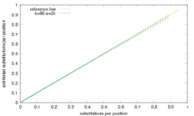
Figure 5: Estimated distances – i.e. estimated average number of substitutions per position – for simulated sequence pairs, plotted against the ‘real’ distances. We used pairs of sequences of length $L=500$ kb and parameters $k=90$ and $w=31$.

	k=30	k=50	k=70	k=90	k=120	k=150	k=200
w=1	0.665	0.809	0.935	0.897	0.794	0.781	0.995
w=5	-	0.839	0.835	0.784	0.783	0.773	0.880
w=11	-	-	0.869	0.808	0.788	0.781	0.863
w=21	-	-	0.813	0.824	0.824	0.804	0.817
w=31	-	-	0.813	0.824	0.824	0.829	0.835
w=51	-	-	-	-	0.824	0.819	0.820

Table 1: Distance values calculated with our algorithm for a pair of simulated sequences of length $L=500$ kb with a match rate of $p=0.5$, corresponding to a distance of $0.824$ substitutions per position. Dashes indicate that no distance value could be calculated since our algorithm could not find the second local maximum in the length distribution of the $k$-mismatch common substrings.

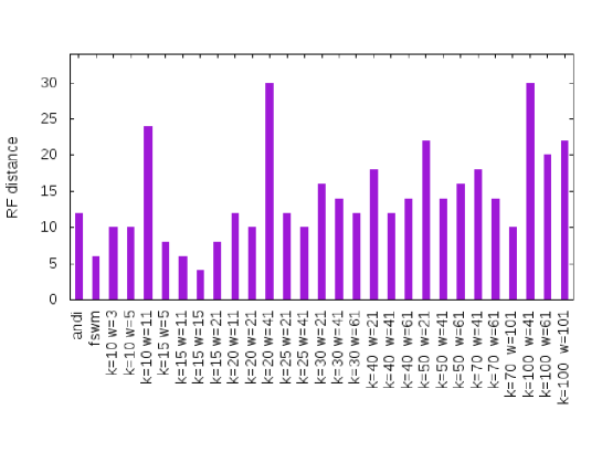
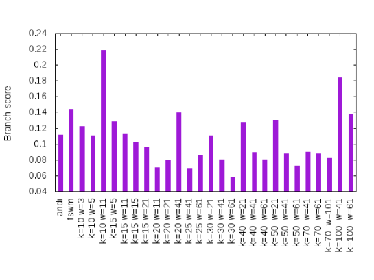
Figure 6: Evaluation of various alignment-free methods for phylogeny reconstruction on on a set of 27 primate mitochondrial genomes. Robinson-Foulds distances (top) and branch scores (bottom) were calculated to measure the difference between the resulting trees and a reference tree obtained with Clustal $\Omega$ and Neighbour Joining.

9 Discussion

In this paper, we introduced a new way of estimating phylogenetic distances between genomic sequences. We showed that the average number of substitutions per position since two sequences have separated from their last common ancestor can be accurately estimated from the position of local maximum in the smoothed length distribution of $k$-mismatch common substrings. To find this local maximum, we used a naive search procedure on the smoothed length distribution. Two parameter values have to be specified in our approach, the number $k$ of mismatches and the size $w$ of the smoothing window for the length distribution. Table 1 shows that our distance estimates are reasonably stable for a range of values of $k$ and $w$.

A suitable value of the parameter $k$ is important to separate the ‘homologous’ peak from the ‘background’ peak in the length distribution of the $k$-mismatch common substrings. As follows from theorem 6.1, the distance between these two peaks is proportional to $k$. The value of $k$ must be large enough to ensure that the homologous peak has a sufficient distance to the background peak to be detectable, see Figure 2. Our data show, on the other hand, that our distance estimates become less precise if $k$ is too large.

Specifying a suitable size $w$ of the smoothing window is also important to obtain accurate distance estimates; a large enough window is necessary to avoid ending up in a local maximum of the raw length distribution. For the data shown in Figure 3, for example, our approach finds the second maximum of the length distribution at 179 if a window width of $w=31$ is chosen. From this value, the match probability $p$ is estimated as

$$\hat{p}=\frac{179+1-90}{179+1}=0.5$$

using equation (16), corresponding to 0.824 substitutions per position according to the Jukes-Cantor formula. This was exactly the value that we used to generate this pair of sequences.

With window lengths of $w=21$ and $w=1$ (no smoothing at all), however, the second local maxima of the length distribution would be found at 181 and 171, respectively, leading to distance estimates of 0.808 ($w=11$) and 0.897 ($w=1$). If the width $w$ of the smoothing window is too large, on the other hand, the second peak may be obscured by the first ‘background’ peak. In this case, no peak is found and no distance can be calculated. In Figure 3, for example, this happens with if a window width $w=51$ is used. Further studies are necessary to find out suitable values for $w$ and $k$, depending on the length of the input sequences.

Finally, we should say that we used a rather naive way to identify possible homologies that are then extended to find $k$-mismatch common substrings. As becomes obvious from the size of the homologous and background peaks in our plots, our approach finds far more background matches than homologous matches. Reducing the noise of background matches should help to find the position of the homologous peak in the length distributions. We will therefore explore alternative ways to find possible homologies that can be used as starting points for $k$-mismatch common substrings.

References

- [1] S. Aluru, A. Apostolico, and S. V. Thankachan. Efficient alignment free sequence comparison with bounded mismatches. RECOMB’12, pages 1–12, 2015.
- [2] A. Apostolico, C. Guerra, G. M. Landau, and C. Pizzi. Sequence similarity measures based on bounded hamming distance. Theoretical Computer Science, 638:76–90, 2016.
- [3] W. I. Chang and E. L. Lawler. Sublinear approximate string matching and biological applications. Algorithmica, 12:327–344, 1994.
- [4] B. Chor, D. Horn, Y. Levy, N. Goldman, and T. Massingham. Genomic DNA -mer spectra: models and modalities. Genome Biology, 10:R108, 2009.
- [5] M. Comin and D. Verzotto. Alignment-free phylogeny of whole genomes using underlying subwords. Algorithms for Molecular Biology, 7:34, 2012.
- [6] J. Felsenstein. PHYLIP - Phylogeny Inference Package (Version 3.2). Cladistics, 5:164–166, 1989.
- [7] D. Gusfield. Algorithms on Strings, Trees, and Sequences: Computer Science and Computational Biology. Cambridge University Press, Cambridge, UK, 1997.
- [8] L. Hahn, C.-A. Leimeister, R. Ounit, S. Lonardi, and B. Morgenstern. rasbhari: optimizing spaced seeds for database searching, read mapping and alignment-free sequence comparison. PLOS Computational Biology, 12(10):e1005107, 2016.
- [9] B. Haubold, F. Klötzl, and P. Pfaffelhuber. andi: Fast and accurate estimation of evolutionary distances between closely related genomes. Bioinformatics, 31:1169–1175, 2015.
- [10] B. Haubold, P. Pfaffelhuber, M. Domazet-Loso, and T. Wiehe. Estimating mutation distances from unaligned genomes. Journal of Computational Biology, 16:1487–1500, 2009.
- [11] B. Haubold, N. Pierstorff, F. Möller, and T. Wiehe. Genome comparison without alignment using shortest unique substrings. BMC Bioinformatics, 6:123, 2005.
- [12] B. Haubold and T. Wiehe. How repetitive are genomes? BMC Bioinformatics, 7:541, 2006.
- [13] M. Höhl, I. Rigoutsos, and M. A. Ragan. Pattern-based phylogenetic distance estimation and tree reconstruction. Evolutionary Bioinformatics Online, 2:359–375, 2006.
- [14] T. H. Jukes and C. R. Cantor. Evolution of Protein Molecules. Academy Press, New York, 1969.
- [15] M. K. Kuhner and J. Felsenstein. A simulation comparison of phylogeny algorithms under equal and unequal evolutionary rates. Molecular Biology and Evolution, 11:459–468, 1994.
- [16] C.-A. Leimeister, M. Boden, S. Horwege, S. Lindner, and B. Morgenstern. Fast alignment-free sequence comparison using spaced-word frequencies. Bioinformatics, 30:1991–1999, 2014.
- [17] C.-A. Leimeister, T. Dencker, and B. Morgenstern. Anchor points for genome alignment based on filtered spaced word matches. arXiv:arXiv:1703.08792[q-bio.GN], 2017.
- [18] C.-A. Leimeister and B. Morgenstern. kmacs: the -mismatch average common substring approach to alignment-free sequence comparison. Bioinformatics, 30:2000–2008, 2014.
- [19] C.-A. Leimeister, S. Sohrabi-Jahromi, and B. Morgenstern. Fast and accurate phylogeny reconstruction using filtered spaced-word matches. Bioinformatics, 33:971–979, 2017.
- [20] U. Manber and G. Myers. Suffix arrays: a new method for on-line string searches. Proceedings of the first annual ACM-SIAM symposium on Discrete algorithms, SODA ’90:319–327, 1990.
- [21] B. Morgenstern, B. Zhu, S. Horwege, and C.-A. Leimeister. Estimating evolutionary distances between genomic sequences from spaced-word matches. Algorithms for Molecular Biology, 10:5, 2015.
- [22] L. Noé. Best hits of 11110110111: model-free selection and parameter-free sensitivity calculation of spaced seeds. Algorithms for Molecular Biology, 12:1, 2017.
- [23] U. F. Petrillo, C. Guerra, and C. Pizzi. A new distributed alignment-free approach to compare whole proteomes. Theoretical Computer Science, in press, 2017.
- [24] C. Pizzi. MissMax: alignment-free sequence comparison with mismatches through filtering and heuristics. Algorithms for Molecular Biology, 11:6, 2016.
- [25] D. Robinson and L. Foulds. Comparison of phylogenetic trees. Mathematical Biosciences, 53:131–147, 1981.
- [26] N. Saitou and M. Nei. The neighbor-joining method: a new method for reconstructing phylogenetic trees. Molecular Biology and Evolution, 4:406–425, 1987.
- [27] F. Sievers, A. Wilm, D. Dineen, T. J. Gibson, K. Karplus, W. Li, R. Lopez, H. McWilliam, M. Remmert, J. Söding, J. D. Thompson, and D. G. Higgins. Fast, scalable generation of high-quality protein multiple sequence alignments using Clustal Omega. Molecular Systems Biology, 7:539, 2011.
- [28] G. E. Sims, S.-R. Jun, G. A. Wu, and S.-H. Kim. Alignment-free genome comparison with feature frequency profiles (FFP) and optimal resolutions. Proceedings of the National Academy of Sciences, 106:2677–2682, 2009.
- [29] S. V. Thankachan, A. Apostolico, and S. Aluru. A provably efficient algorithm for the -mismatch average common substring problem. Journal of Computational Biology, 23:472–482, 2016.
- [30] S. V. Thankachan, S. P. Chockalingam, Y. Liu, A. Apostolico, and S. Aluru. ALFRED: a practical method for alignment-free distance computation. Journal of Computational Biology, 23:452–460, 2016.
- [31] S. V. Thankachan, S. P. Chockalingam, Y. Liu, A. Krishnan, and S. Aluru. A greedy alignment-free distance estimator for phylogenetic inference. BMC Bioinformatics, 18:238, 2017.
- [32] I. Ulitsky, D. Burstein, T. Tuller, and B. Chor. The average common substring approach to phylogenomic reconstruction. Journal of Computational Biology, 13:336–350, 2006.
- [33] S. Vinga. Editorial: Alignment-free methods in computational biology. Briefings in Bioinformatics, 15:341–342, 2014.
- [34] S. Vinga, A. M. Carvalho, A. P. Francisco, L. M. S. Russo, and J. S. Almeida. Pattern matching through Chaos Game Representation: bridging numerical and discrete data structures for biological sequence analysis. Algorithms for Molecular Biology, 7:10, 2012.
- [35] H. Yi and L. Jin. Co-phylog: an assembly-free phylogenomic approach for closely related organisms. Nucleic Acids Research, 41:e75, 2013.