Hybrid Particle-Continuum Simulations Coupling Brownian Dynamics and Local Dynamic Density Functional Theory

Abstract

We present a multiscale hybrid particle-field scheme for the simulation of relaxation and diffusion behavior of soft condensed matter systems. It combines particle-based Brownian dynamics and field-based local dynamics in an adaptive sense such that particles can switch their level of resolution on the fly. The switching of resolution is controlled by a tuning function which can be chosen at will according to the geometry of the system. As an application, the hybrid scheme is used to study the kinetics of interfacial broadening of a polymer blend, and is validated by comparing the results to the predictions from pure Brownian dynamics and pure local dynamics calculations.

I Introduction

Dynamical processes in soft materials are typically characterized by multiple time and length scales, an intrinsic feature that brings significant challenge for the design of efficient simulation schemes multiscale_bridge ; multscale_rev . Although the computational power still continuously increases each year, studying macroscopic properties of polymer systems by atomistic simulations has remained infeasible. Therefore, to study processes on larger time and length scales, coarse-grained (CG) models have been developed as well as multiscale modelling schemes where different length scales are coupled concurrently. Among these simulation techniques, hybrid adaptive resolution schemes are particularly useful, since in such schemes most parts of the system are represented by a lower resolution model, to save time, while the detailed description holds only where it is required, to keep accuracy. Depending on the concrete representation schemes, the hybrid models may be categorized into hybrid particle-particle methods (HPP)AM_CG1 ; AM_CG_H ; AM_CG_H1 ; AdResS1 ; QM_CG1 ; QM_CG2 ; Adaptive_reservoir ; H_AdResS , where both the fine-grained and coarse-grained description are constructed using particle-based models, and hybrid particle-continuum (or particle-field) (HPF) methods, where the fine-grained molecules are resolved by particles while the coarse-grained molecules are represented by some continuum quantities which are controlled by some continuous dynamic equations HybridMD1 ; HybridMD2 ; triple_scale ; MD_FH1 ; MD_FH2 ; HPF1 ; HPF2 . Well-known examples of HPP schemes are the hybrid QM/MM methods QM_MM or the hybrid atomistic-CG approaches AM_CG1 ; AM_CG_H ; AM_CG_H1 ; AdResS1 . HPF schemes include hybrid particle-density functional schemes HPF1 ; HPF2 and hybrid schemes linking molecular dynamics and fluctuating hydrodynamics (MD/FH)HybridMD1 ; HybridMD2 ; MD_FH1 ; MC_NS . However, so far, the HPF schemes have either been restricted to static properties - such as, e.g., the Monte Carlo scheme proposed by us in previous work HPF1 - or to fluids of small molecules - such as, e.g., the MD/FH schemes where molecular fluids are connected to Navier-Stokes fluids via buffer zonesHybridMD1 ; MD_FH1 ; MD_FH2 ; MD_SDPD1 ; MD_SDPD2 ; MD_MCD .

In the present paper, the HPF will refer to adaptive resolution models where materials are represented at different levels – particle or field – in different spatially separated domains, as explained above. However, we should note that in the literature, the term “hybrid particle-field modeling” is also used for a variety of other, intrinsically different models:

Originally, the idea of hybrid particle-field modeling was exploited for the study of two-component systems with one component described by a particle-based model while the other uses a field model. For example, in the late 90s, Miao et al brush_shear and Saphiannikova et al brush_NS proposed a mixed scheme to study the conformational properties of polymer brushes under shear. They utilized the continuous Brinkman equation (a variant of the Navier-Stokes equation) to describe the motion of the solvent, and Brownian dynamics (BD) to simulate polymer brushes. Similar ideas were later adopted by Sides et al HPF_Sides , with the difference that they focussed on a colloid-polymer composite, and treated polymers as continuous fields and colloids as Brownian particles. The main feature of these hybrid approaches is that different resolution schemes are chosen for specified components at the very beginning, and these representations do not change during the simulation.

Ganesan and coworkers BD_DMFT ; BD_DSCF and Milano and Kawakatsu Milano1 ; Milano2 ; Milano3 introduced another type of single-resolution “hybrid particle-field modeling”, where the fields are essentially used to define the interactions between particles. The whole simulation is controlled by a particle-based BD or MD algorithm, while the fields, e.g., densities, appear as intermediate variables, i.e., they are extracted from all the particle positions and then used for the calculation of interaction forces. The introduction of these fields can be viewed as a way to efficiently deal with nonbonded molecular interactions. A similar approach was first proposed by Laradji et al Laradji ; off_lattice , and also characterizes the “single chain in mean field theory” SCMF1 ; SCMF2 .

In contrast, the MD/FD approach first proposed by de Fabritiis et al HybridMD1 ; HybridMD2 is a ”true” HPF model with adaptive resolution, which which combines particle-based MD simulations and continuum-based fluctuating hydrodynamic models dynamically. In this model the stochastic equations are integrated by numerical methods of computational fluid dynamics. Mass and momentum conservations are achieved through flux balance restriction. Later, this HPF scheme was combined with an HPP (atomistic/CG) model leading to a triple-scale approach triple_scale . Similar MD/FD schemes using other Navier-Stokes solvers have been proposed, e.g., methods based on smoothed dissipative particle dynamics MD_SDPD1 ; MD_SDPD2 or on multiparticle collision dynamics MD_MCD .

Recently, we have developed a different HPF method which is specifically designed for large, complex molecules, i.e., polymers. It couples a particle region to a field region where the thermodynamics is described by polymer density functional theory HPF1 ; HPF2 . The simulation algorithm uses a combination of Monte Carlo (MC) moves and field relaxation steps. We have shown how to construct such hybrid models systematically by field-theoretic methods. The derivation is based on the fact that the particle representation and field representation originate from the same partition function obtained from the same Edwards Hamiltonian Edwards1 ; Edwards2 ; Edwards3 ; Edwards4 . Thus in principle, the particle description, the field description, and the derived hybrid description are almost equivalent and should give the same macroscopic thermodynamic properties. This equivalence has been verified within statistical errors through the study of polymer conformation properties in a solution HPF2 and effective interactions between two polymer grafted colloids immersed in a diblock copolymer melt HPF1 . However, so far the method cannot be used to study dynamical processes.

In this paper, we extend our previous static model and move one step forward to construct a dynamic hybrid HPF scheme for the simulation of systems with diffusive dynamics. The scheme ensures local mass conservation, but it neglects inertia effects and thus does not account for momentum conservation. Therefore, it is suited for studying relaxational dynamics and diffusion behavior in systems where hydrodynamic interactions are not important. More specifically, particles move according to Brownian dynamics (BD), and fields are propagated according to the equations of local dynamic density functional theory (LD) LD1 ; LD2 ; LD3 . Polymers can switch between different levels of resolution on the fly. These ”resolution switches” are controlled by a chemical potential like function, i.e., a tuning function, rather than by a force or potential interpolation as in other adaptive resolution models. The switch process is constructed such that local mass conservation is guaranteed. We illustrate the method at the example of a study of interface broadening in an A/B polymer blend.

The remainder of the paper is organized as follows: In Sec II, we describe our methodology at the example of a polymer solution with implicit solvent. The three components of our hybrid scheme, the BD method (II.1), the LD method (II.2) and identity switches (II.3) are discussed separately. In Sec III, we present simulation results. We first test the constructed hybrid scheme using the polymer solution and then utilize it to study the interdiffusion process of a polymer blend. We close with a brief summary in Sec IV.

II Hybrid Particle-Field Scheme: Methodology

In this section we describe in detail the construction of the HPF model. For simplicity, we focus on a solution of homopolymer Gaussian chains. The extension to more complicated polymers or copolymers and to mixtures etc. is straightforward.

We consider a system containing $n_{\mathrm{t}}$ Rouse polymers of length $N$ confined in a cubic box of volume $V=L_{\mathrm{x}}\cdot L_{\mathrm{y}}\cdot L_{\mathrm{z}}$ with periodic boundary conditions. In the following and throughout the paper, we give all lengths in units of the radius of gyration of a free Gaussian chain $R_{\mathrm{g}}=\sqrt{Nb^{2}/6}$, where $b$ is the statistical Kuhn length, energies in units of $k_{B}T$, where $k_{B}$ is the Boltzmann constant and $T$ the temperature, and times in units of the relaxation time of a single chain, i.e., $t_{0}=R^{2}_{\mathrm{g}}/D_{\mathrm{c}}$, where $D_{\mathrm{c}}$ is the mobility of the center of mass of a single chain. The original Hamiltonian of the system is written as the sum of two contributions $\mathcal{H}=\mathcal{H}_{0}+\mathcal{H}_{\mathrm{I}}$, where $\mathcal{H}_{0}$ accounts for the chain connectivity and the bonded intrachain interactions, and $\mathcal{H}_{\mathrm{I}}$ represents the nonbonded interactions between chain monomers. Written in terms of local densities, it has the form Edwards1 ; Edwards2 ; Edwards3 ; Edwards4

$$\mathcal{H}_{\mathrm{I}}=\frac{n_{\mathrm{t}}v_{\mathrm{ex}}}{2V}\int d\mathbf{r}\hat{\phi}^{2},$$ (1)

where $v_{\mathrm{ex}}$ is the excluded volume parameter, and $\hat{\phi}(\mathbf{r})\equiv\frac{1}{\rho_{0}}\sum_{\mathrm{mj}}\delta(\mathbf{r}-\mathbf{R}_{\mathrm{mj}})$ is the normalized microscopic density with respect to the total mean monomer density $\rho_{0}=n_{\mathrm{t}}N/V$.

In the HPF scheme, the chains are first partitioned into ”particle type chains” (p-chains) and ”field type chains” (f-chains), depending on the state of virtual internal degrees of freedom as described below in Sec II.3. The f-chains are then turned into fluctuating density fields by a field-theoretic transformation and a saddle-point integrationHong ; SCF1 ; HPF1 ; HPF2 . This results in an effective free energy functional of the form

$$\mathcal{F}[\{\mathbf{R}_{\mathrm{mj}}\},\phi_{\mathrm{f}}]=\mathcal{F}_{0,\mathrm{p}}[\{\mathbf{R}_{\mathrm{mj}}\}]+\mathcal{F}_{0,\mathrm{f}}[\phi_{\mathrm{f}}]+\mathcal{F}_{\mathrm{I}}[\{\mathbf{R}_{\mathrm{mj}}\},\phi_{\mathrm{f}}]$$ (2)

for the particle-field system, which depends on the positions $\{\mathbf{R}_{\mathrm{mj}}\}$ of p-chain monomers – the index m refers to the molecule, and the index j to the monomer in the chain – and on the local densities $\phi_{f}$ of f-chain monomers. The terms $\mathcal{F}_{0,\mathrm{p}}$ and $\mathcal{F}_{0,\mathrm{f}}$ include the contributions of the intrachain interactions and the chain entropy of p-chains and f-chains, respectively, and $\mathcal{F}_{I}$ describes the bonded interactions, which is derived from (1) and given by

$$\mathcal{F}_{\mathrm{I}}=\frac{n_{\mathrm{t}}v_{\mathrm{ex}}}{2V}\int d\mathbf{r}\>(\phi_{\mathrm{f}}+\hat{\phi}_{\mathrm{p}})^{2}.$$ (3)

in a homopolymer solution. Here $\hat{\phi}_{\mathrm{p}}(\mathbf{r})$ of course refers to the normalized local density of p-chains only.

For Gaussian chains, $\mathcal{F}_{0,\mathrm{p}}$ can be written as Doi

$$\mathcal{F}_{0,\mathrm{p}}=\frac{N}{4}\sum_{\mathrm{m}=1}^{n_{\mathrm{p}}}\sum_{j=2}^{\mathrm{N}}\big{(}\mathbf{R}_{\mathrm{mj}}-\mathbf{R}_{\mathrm{m,j-1}}\big{)}^{2}.$$ (4)

The sum m runs over the p-chains and $\mathbf{R}_{\mathrm{mj}}$ is the position of the jth bead of the mth chain.

Finally, the intrachain contribution of f-chains to the free energy, $\mathcal{F}_{0}^{\mathrm{f}}$, takes the general form

$$\mathcal{F}_{0,\mathrm{p}}=-\frac{n_{\mathrm{t}}}{V}\int d\mathbf{r}\>\phi_{\mathrm{f}}\>\omega_{\mathrm{f}}-n_{\mathrm{f}}\ln[Q_{\mathrm{f}}V],$$ (5)

where $\omega_{\mathrm{f}}(\mathbf{r})$ are conjugate fields defined such that hypothetical external potentials $W=\frac{1}{N}\omega_{\mathrm{f}}$ would generate exactly the f-density configuration $\phi_{\mathrm{f}}(\mathbf{r})$ in a reference system of noninteracting f-chains, and $\mathcal{Q}_{\mathrm{f}}$ is the partition function of a single chain subject to such potentials $W_{\mathrm{f}}$. For Gaussian chains, it is given by

$$\mathcal{Q}_{\mathrm{f}} = \frac{1}{Z_{0}}\int\mathrm{d}\bf R_{1}\cdots\mathrm{d}\bf R_{N}$$

$$\times \exp\Big{\{}-\frac{N}{4}\sum_{j=2}^{N}(\mathbf{R}_{j}-\mathbf{R}_{j-1})^{2}-\frac{1}{N}\sum_{j=1}^{N}\omega(\mathbf{R}_{j})\Big{\}}.$$

We note that in this formalism, $\phi_{\mathrm{f}}$ is the only free field, and $\omega_{\mathrm{f}}$ must be determined from $\phi_{\mathrm{f}}$. An explicit relation between $\phi_{\mathrm{f}}$ and $\omega_{\mathrm{f}}$ can be obtained through the following procedure: We define an end-integrated single chain propagator $q_{\mathrm{f}}(\mathbf{r},s)$, which satisfies the modified diffusion equation SCF1 ; SCF2

$$\frac{\partial q_{\mathrm{f}}}{\partial s}=\nabla^{2}q_{\mathrm{f}}-\omega_{\mathrm{f}}q_{\mathrm{f}},$$ (7)

where $s$ is a normalized chain contour variable ranging from 0 to 1. The propagator of $q_{\mathrm{f}}$ is then calculated numerically with initial condition $q_{\mathrm{f}}(\mathbf{r},0)=1$ and periodic boundary conditions, e.g., using a pseudo-spectral method. Knowing the propagator $q_{\mathrm{f}}$, one can calculate the single chain partition function via $Q_{\mathrm{f}}=\frac{1}{V}\int d\mathbf{r}\>q_{\mathrm{f}}(\mathbf{r},1)$, and the density field via SCF1 ; SCF2

$$\phi_{\mathrm{f}}=\frac{\bar{\phi}_{\mathrm{f}}}{Q_{\mathrm{f}}}\int_{0}^{1}ds\>q_{\mathrm{f}}(\mathbf{r},s)\>q_{\mathrm{f}}(\mathbf{r},1-s).$$ (8)

The functional inversion to get $\omega_{\mathrm{f}}$ from $\phi_{\mathrm{f}}$ (density targeting problem) is done numerically using iteration techniques. Several iteration schemes are available; for more details, see, e.g., target_density ; fluctuation_dynamics ; stasiak .

In the dynamic HPF scheme, the motion of the particle-resolved p-chains is described by BD dynamics, whereas the density profiles of the coarse-grained f-chains evolve according to a dynamic density functional, the LD scheme. The switches between p-chains and f-chains are controlled by a predefined tuning function. Apart from the switches, the system is propagated by numerical integration of the BD equations of motion (p-chains) and the LD equation (f-chains). More concretely the evolution of the system in each integration step is composed of three independent steps. First, all the beads’ positions of p-chains are updated according to the BD equations, second, density profiles are evolved according to the LD equations, and third, a finite number of identity switches are carried out controlled by a Monte Carlo (MC) criterion. An advantage of completely decoupling the updating and the switching process is that the hybrid algorithm becomes more flexible with respect to incorporating other dynamic models, and can be extended to other polymer models more easily. In the following we describe the BD dynamics, the LD method, and the switching algorithm respectively.

II.1 Particle Propagation: Brownian Dynamics

The motion of particle beads (in p-chains) is driven by a conservative force derived from the Hamiltonian and a random force originating from the thermal fluctuations, i.e.,

$$\frac{d\mathbf{R}_{\mathrm{mj}}}{dt}=-D_{0}\frac{\partial\mathcal{F}}{\partial\mathbf{R}_{\mathrm{mj}}}+\sqrt{2D_{0}}\mathbf{f}_{\mathrm{mj}},$$ (9)

with $D_{0}=1/N$ (in units of $R^{2}_{\mathrm{g}}/t_{0}$). The random force $\mathbf{f}_{\mathrm{mj}}$ is Gaussian distributed with zero mean and variance $\langle f_{\mathrm{mjI}}(t)f_{\mathrm{nkJ}}(t^{\prime})\rangle=\delta_{\mathrm{mn}}\delta_{\mathrm{jk}}\delta_{\mathrm{IJ}}$ where I,J denote the Cartesian components. The derivative of Hamiltonian over particle positions can be performed directly using the chain rule and properties of the delta function. The result can be formally written as slowdown

$$\frac{\partial\mathcal{H}}{\partial\mathbf{R}_{\mathrm{mj}}}=\frac{N}{2}\big{(}\mathbf{R}_{\mathrm{mj}}-\mathbf{R}_{\mathrm{m,j+1}}-\mathbf{R}_{\mathrm{m,j-1}}\big{)}+\frac{1}{N}\frac{\partial\hat{\omega}_{\mathrm{p}}}{\partial\mathbf{R}_{\mathrm{mj}}},$$ (10)

where $\hat{\omega}_{\mathrm{p}}$ can be viewed as the conjugate potential to $\hat{\phi}_{\mathrm{p}}$, and is obtained as

$$\hat{\omega}_{\mathrm{p}}=v_{\mathrm{ex}}(\hat{\phi}_{\mathrm{p}}+\phi_{\mathrm{f}})$$ (11)

in our homopolymer solution. Therefore the nonbonded force acting on one bead is evaluated through the derivative of densities with respect to the bead’s position.

In practice, all densities are discretized, and they are extracted by a “particle-to-mesh” assignment function. To do so, we uniformly divide the simulation box into $n_{\mathrm{x}}\cdot n_{\mathrm{y}}\cdot n_{\mathrm{z}}$ cells, and define all densities on the vertexes (mesh points) of these cells. Several choices of the assignment function PM are possible. The zeroth order scheme is the so called the nearest-grid scheme MC_brush1 , which assigns a bead to its nearest mesh point. Here we adopt a linear order scheme, which assigns fractions of a bead to its eight nearest mesh points, the so-called cloud-in-cell (CIC) scheme MC_brush2 ; CIC . In the CIC scheme, the fraction assigned to a given vortex is proportional to the volume of a rectangular whose diagonal is the line connecting the partition position and the mesh point on the opposite side of the cell. The assignment function completely determines the finite-differential form of the derivative of $\hat{\omega}_{\mathrm{p}}$. The nonbonded force acting on a bead is finally expressed as the linear interpolation of $\hat{\omega}_{\mathrm{p}}$ defined on the bead’s eight nearest mesh points with weights calculated according to the distance between the particle and the mesh point. As the explicit form of the assignment function and the nonbonded force are extensively discussed elsewhere, we just refer to Refs.slowdown ; PM .

II.2 Field Propagation: Local Dynamic Density Functional

The density fields $\phi_{\mathrm{f}}$ of f-chains are propagated according to a dynamic density functional. The starting point is the continuity equation for the monomer densities $\rho_{0}\frac{\partial\phi_{\mathrm{f}}}{\partial t}=-\nabla\mathbf{j}$, where the current $\mathbf{j}$ is driven by the thermodynamic force $\nabla\mu_{\mathrm{f}}$ with $\mu_{\mathrm{f}}:=\frac{\delta\mathcal{F}}{\delta\phi_{\mathrm{f}}}$ fluctuation_dynamics . Here we use a local dynamics scheme, where the thermodynamic force and the flux are linearly related, $\mathbf{j}=-D_{c}N\rho_{0}\phi_{\mathrm{f}}\nabla\mu_{\mathrm{f}}$, leading to the LD equation LD1 ; LD2 ; LD3 :

$$\frac{\partial\phi_{\mathrm{f}}}{\partial t}=D_{c}\nabla\cdot\Big{[}\phi_{\mathrm{f}}\nabla\frac{\delta\mathcal{F}}{\delta\phi_{\mathrm{f}}}\Big{]}$$ (12)

with $\delta\mathcal{F}/\delta\phi_{\mathrm{f}}=\frac{n_{\mathrm{t}}}{V}[v_{\mathrm{ex}}(\hat{\phi}_{\mathrm{p}}+\phi_{\mathrm{f}})-\omega_{\mathrm{f}}]$ in the case of the homopolymer soluation.

In the present work, the LD equation is integrated numerically using the explicit Euler scheme, and the derivatives are evaluated in Fourier space using fast Fourier transform (FFT) FFT . To perform the numerical calculations, we discretize all the continuum quantities and define them only on the mesh points for convenience. Thus the space decomposition used in the LD dynamics is the same as that used in the BD simulation when calculating the densities.

II.3 Chain Identity Switches

Originally, all $n_{\mathrm{t}}$ chains in the system are identical. For the HPF modeling, we need to first partition these chains into p-chains and f-chains. There are several ways to do the partitioning. The strategy we adopt here is based on the introduction of an additional “spin” variable $\tau_{\mathrm{mj}}$, which is attached to each bead as an identifier HPF1 ; HPF2 . The spin $\tau_{\mathrm{mj}}$ can take a value either 0 or 1. A chain is identified as an f-chain if all the spins on this chain are set zero, otherwise it is a p-chain. We note that this partioning method leads to the asymmetry of p-chains and f-chains in the spin space, where p-chains have a larger spin entropy. To control the value of $\tau_{\mathrm{mj}}$, we further introduce a tuning function $\Delta\mu(\mathbf{r})$, which plays the role of the spin’s conjugate potential. The tuning function couples to $\tau_{\mathrm{mj}}$, and thus determines the distributions of p-chain and f-chains. Therefore, p-chains and f-chains are treated as two chemically different species, and $\Delta\mu$ acts similar to a chemical potential difference, which however varies locally. From a technical point of view, we thus work in a semi-grand canonical ensemble.

In the present study, the tuning function is imposed externally and must be specified beforehand. Some general considerations can help to construct an appropriate form for $\Delta\mu$. For example, it should be chosen such that p-chains appear only in specific regions (e.g., near boundaries), where a detailed description is required, while in the remaining large region, chains are represented by coarse-grained fields. Based on such considerations, an optimal form of $\Delta\mu$ may be constructed that it is in compatible with the geometry of the localized region as well as the whole system.

The chain identity switches are driven by the tuning function, and to sample the spin variable, we adopt a Monte Carlo type scheme book_MC1 ; book_MC2 . It is motivated by the following consideration: We require that a spin variable $\tau$ on a bead at position $\mathbf{r}$ assumes the value $\tau=1$ with a probability $w_{1}$ roughly given by HPF1 ; HPF2

$$w_{1}=\frac{e^{\Delta\mu(\mathbf{r})}}{1+e^{\Delta\mu(\mathbf{r})}}$$ (13)

while the probability for $\tau=0$ is $w_{0}=1-w_{1}$. In the absence of other dynamical processes (BD or LD moves), this probability distribution can be generated exactly with the following algorithm:

1. We generate a random number in the interval $[0,n_{\mathrm{p}}\cdot M+n_{\mathrm{f}}$, where $M$ is an integer used to increase the probability of choosing a p-chain, which is introduced to at least partly account for the large spin entropy of p-chains. If the integer generated is smaller than $n_{\mathrm{p}}\cdot M$, we choose a p-chain, otherwise we manipulate an f-chain.

2. Suppose that the mth p-chain is chosen (with probability $\frac{M}{n_{\mathrm{p}}\cdot M+n_{\mathrm{f}}}$), we then randomly single out a bead j in this chain (the probability that the ith bead being chosen $1/N$), and subsequently we flip the bead’s identity.

   If $\tau_{\mathrm{mj}}=0$, we attempt to change it to $\tau_{\mathrm{mj}}=1$. According to the definition of the p-chains, in this case, the p-chain is still a p-chain after the switch. We write the transition probability of such a switch as

   $$P^{\mathrm{pp}}(0\to 1)=\frac{M}{n_{\mathrm{p}}\cdot M+n_{\mathrm{f}}}\frac{1}{N}W^{\mathrm{pp}}_{01},$$ (14)

   where $W^{\mathrm{pp}}_{01}$ denotes the acceptance probability, which will be specified below.

   If $\tau_{\mathrm{mj}}=1$, we try to flip it to $\tau_{\mathrm{mj}}=0$. The chain type (p-chain or f-chain) after the switch depends on the spin values of all other beads. We have to distinguish between two different cases.

   In the first case, at least one other bead (say the lth bead) carries a spin $\tau_{\mathrm{ml}}=1$. After the switch, the chain is then still a p-chain. The transition probability is

   $$P^{\mathrm{pp}}(1\to 0)=\frac{M}{n_{\mathrm{p}}\cdot M+n_{\mathrm{f}}}\frac{1}{N}W^{\mathrm{pp}}_{10},$$ (15)

   where $W^{\mathrm{pp}}_{10}$ is again an acceptance probability.

   In the second case, we have $\tau_{\mathrm{ml}}=0$ for all $l\neq j$, and the switch will change this p-chain to an f-chain. The transition probability for such a switch is written as

   $$P^{\mathrm{pf}}_{\mathrm{j}}[\{\mathbf{R}_{\mathrm{mj}}\}]=\frac{M}{n_{\mathrm{p}}\cdot M+n_{\mathrm{f}}}\frac{1}{N}W^{\mathrm{pf}}_{\mathrm{j}}.$$ (16)

   Here, $P^{\mathrm{pf}}_{\mathrm{j}}$ and the acceptance probability $W^{\mathrm{pf}}_{\mathrm{j}}$ may depend on the conformation $\{\mathbf{R}_{\mathrm{mj}}\}$ of the chain m.

3. If an f-chain has been picked in step 1 (with probability $\frac{n_{\mathrm{f}}}{n_{\mathrm{p}}\cdot M+n_{\mathrm{f}}}$), we attempt to switch it to a p-chain. To do so we first choose a bead j (with probability $1/N$) and a location $\mathbf{r}$ according to a probability $H_{\mathrm{j}}(\mathbf{r})$, and then generate a trial bead at the position $\mathbf{r}$. In case the move is accepted, this bead becomes the j-th bead of a p-chain and replaces the j-th bead of an f-chain. Hence the probability of picking that f-bead is $H_{\mathrm{j}}(\mathbf{r})/\rho_{0}\phi_{\mathrm{f,j}}(\mathbf{r})\Delta V$, where $\Delta V$ is the volume of a cell, and $\rho_{0}\phi_{\mathrm{f,j}}$ the density of j-th monomers of f-chains. Then we construct a Gaussian chain with jth bead fixed at $\mathbf{r}$. The a priori probability $P_{\mathrm{priori}}$ to generate a given set of coordinates $\{\mathbf{R}_{\mathrm{k}}\}$ is

   $$P_{\mathrm{priori}}[\{\mathbf{R}_{\mathbf{k}}\}]=\frac{1}{Z_{0}}\exp\Big{[}-\frac{N}{4}\sum_{j=2}^{\mathrm{N}}\big{(}\mathbf{R}_{\mathrm{j}}-\mathbf{R}_{\mathrm{j-1}}\big{)}^{2}\Big{]},$$ (17)

   where the normalization factor $\mathcal{Z}_{0}=(\frac{N}{4\pi})^{3(N-1)/2}$ corresponds to te partition function of an ideal noninteracting reference chain of length $N$. The transition probability from an f-chain to this p-chain is thus expressed as

   $$P^{\mathrm{fp}}[\{\mathbf{R}_{\mathrm{k}}\}]=\frac{n_{\mathrm{f}}}{n_{\mathrm{p}}\cdot M+n_{\mathrm{f}}}\frac{H_{\mathrm{j}}}{\rho_{0}\phi_{\mathrm{f,j}}\Delta V}P_{\mathrm{priori}}\>W^{\mathrm{fp}}_{\mathrm{j}},$$ (18)

   with the acceptance probability $W^{\mathrm{fp}}_{\mathrm{j}}$, which again may depend on the conformation of the new p-chain.

4. The trial move is accepted with probability $W^{\mathrm{pp}}_{01}$, $W^{\mathrm{pp}}_{10}$, $W^{\mathrm{pf}}_{\mathrm{j}}$, or $W^{\mathrm{fp}}_{\mathrm{j}}$, respectively. To ensure local mass conservation, this is done in a manner that the total density $\hat{\phi}_{\mathrm{p}}(\mathbf{r})+\phi_{\mathrm{f}}(\mathbf{r})$ is preserved everywhere. Hence, if a switch from the mth p-chain to the mth f-chain is accepted, we remove its previous contribution to the density, say $\hat{\phi}_{\mathrm{m}}$ from $\hat{\phi}_{\mathrm{p}}$, and add it to $\phi_{\mathrm{f}}$. This also entails the calculation of the new $\omega_{f}$ which gives $\phi_{\mathrm{f}}+\phi_{\mathrm{m}}$. Similarly, if the switch from an f-chain to a p-chain is accepted, we remove the density distribution of the newly generated p-chain from $\phi_{\mathrm{f}}$ and update $\omega_{\mathrm{f}}$ accordingly.

If only switch moves are made, the target spin distribution (13) can be obtained by choosing the acceptance probabilities $W^{\mathrm{pp}}_{01}$, $W^{\mathrm{pp}}_{10}$, $W^{\mathrm{pf}}_{\mathrm{mf}}$, and $W^{\mathrm{fp}}_{\mathrm{j}}$ such that they satisfy the detailed balance condition. In the case of p-p switches, this condition simply reads $w_{0}P^{\mathrm{pp}}_{01}=w_{1}P^{\mathrm{pp}}_{10}$, and it can be implemented with the simple Metropolis criterion

$$W^{\mathrm{pp}}_{01}=\min(1,e^{-\Delta\mu}),\;W^{\mathrm{pp}}_{10}=\min(1,e^{\Delta\mu}).$$ (19)

In the case of p-f or f-p switches, one must account for the entropy gain associated with the replacement of an actual p-chain m with density distribution $\hat{\phi}_{\mathrm{m}}$ by a f-chain density distribution $\phi_{\mathrm{m}}$. The corresponding free energy difference is given by $\Delta\mathcal{F}_{0}=\Delta\mathcal{F}_{0,\mathrm{p}}+\Delta\mathcal{F}_{0,\mathrm{f}}$ with $\Delta\mathcal{F}_{0,\mathrm{p}}=-\frac{N}{4}\sum_{j=2}^{\mathrm{N}}\big{(}\mathbf{R}_{\mathrm{j}}-\mathbf{R}_{\mathrm{j-1}}\big{)}^{2}$ and $\Delta\mathcal{F}_{0,\mathrm{f}}=\mathcal{F}_{0,\mathrm{f}}[\phi_{\mathrm{f}}+\phi_{\mathrm{m}}]-\mathcal{F}_{0,\mathrm{f}}[\phi_{\mathrm{f}}]$, where $\phi_{\mathrm{f}}$ denotes the density distribution of f-chains without the chain $m$. Thus the detailed balance condition reads

$$w_{1}P^{\mathrm{pf}}_{\mathrm{j}}=w_{0}P^{\mathrm{fp}}_{\mathrm{j}}\>e^{-\Delta\mathcal{F}_{0}},$$ (20)

which can be achieved with the Metropolis form

$$W^{\mathrm{pf}}_{\mathrm{j}} = \min(1,e^{-\Delta\mu-\Delta\mathcal{F}_{0,\mathrm{f}}}\frac{H_{\mathrm{j}}(\mathbf{r}_{\mathrm{j}})}{Z_{0}\rho_{0}\phi_{\mathrm{f,j}}(\mathbf{r}_{\mathrm{j}})\Delta V})$$ (21)

$$W^{\mathrm{fp}}_{\mathrm{j}} = \min(1,e^{\Delta\mu+\Delta\mathcal{F}_{0,\mathrm{f}}}\frac{Z_{0}\rho_{0}\phi_{\mathrm{j}}(\mathbf{r}_{\mathrm{j}})\Delta V}{H_{\mathrm{j}}(\mathbf{r}_{\mathrm{j}})}).$$

With this choice of acceptance probabilities, one would obtain the target spin distribution (13) in a simulation that only includes spin switches, i.e., chain identity switches. However, the expressions (21) are quite complicated and involve time consuming calculations of $\Delta\mathcal{F}_{0,\mathrm{f}}$ and $\phi_{\mathrm{f,j}}$. On the other hand, an exact implementation of a target spin distribution is not truly necessary, since the spins are auxiliary variables and have no physical meaning. Moreover the BD and LD moves described in Secs II.1 and II.2 distort the spin distribution anyway, since they do not satisfy detailed balance with respect to (13). Therefore, we have chosen to simplify the expressions (21) by making the following approximations: First, we replace $\Delta\mathcal{F}_{0,\mathrm{f}}\approx-\ln(Z_{0})$. Second, we neglect the fact that $\rho_{0}\phi_{\mathrm{f,j}}$ depends on j, i.e., we approximate $\rho_{0}\phi_{\mathrm{f,j}}\approx\frac{1}{N}\rho_{0}\phi_{\mathrm{j}}$, and choose $H_{\mathrm{j}}(\mathbf{r})\equiv H(\mathbf{r})=\rho_{0}\phi_{\mathrm{f}}(\mathbf{r})$ in step 3. With these simplifications, the acceptance probability (21) takes the simple form

$$W^{\mathrm{pf}}=\min(1,e^{-\Delta\mu}),\;W^{\mathrm{fp}}=\min(1,e^{\Delta\mu}).$$ (22)

in analogy to Eq. (19).

III Results and discussion

III.1 Chain partitioning in a polymer solution

We first test the partitioning of p-chains and f-chains driven by the tuning function in a homogeneous polymer solution with periodic boundary conditions. We choose the total number of chains $n_{\mathrm{t}}=10^{4}$, and chain length $N=20$ for all chains. Initially, we set $n_{\mathrm{p}}=n_{\mathrm{f}}=5000$, and the configurations of p-chains are generated randomly as Gaussian coils, while the field density is set to be homogeneous. The size of the box is $L_{\mathrm{x}}=L_{\mathrm{y}}=2$, and $L_{\mathrm{z}}=16$ with discretization $n_{\mathrm{x}}=n_{\mathrm{y}}=8$, and $n_{\mathrm{z}}=64$, i.e., we have uniform cubic cells with volume 0.125. The average number of beads in each cell is about 50, which should be large enough to generate smooth densities. The excluded volume parameter is set $v_{\mathrm{ex}}=1$.

To integrate the dynamic equations numerically, we choose a multiple time step approach with time step $\Delta t_{\mathrm{BD}}=5\times 10^{-4}t_{0}/N$ for the BD scheme, and $\Delta t_{\mathrm{LD}}=10^{-4}t_{0}$ for the LD equation. During each evolution step, we thus update f-chains one time and p-chains 4 times, i.e. we have $\Delta t\equiv\Delta t_{\mathrm{LD}}=4\Delta t_{\mathrm{BD}}$. In each simulation step, after updating the p-chains and f-chains, we attempt to switch beads $S=500$ times, and about 10 chains are successfully switched. The parameter used to enhance the probability of finding a p-chain is set to $M=20$. With these parameters, the density profiles for p-chains and f-chains reach equilibrium within about half the relaxation time $t_{0}$ of a single chain.

In principle, the tuning function can be chosen at will. In our test, we assume that $\Delta\mu$ depends only on $z$ and has an almost steplike profile,

$$\Delta\mu(z)=\frac{\mu_{\mathrm{b}}+\mu_{\mathrm{m}}}{2}+\frac{\mu_{\mathrm{b}}-\mu_{\mathrm{m}}}{2}\tan\Big{[}\eta\cos\frac{2\pi}{L_{\mathrm{z}}}\Big{(}z-\frac{L_{\mathrm{z}}}{2}\Big{)}\Big{]}$$ (23)

where $\mu_{\mathrm{b}}=0$, $\mu_{\mathrm{m}}=-1$, $\eta=10$ are parameters determining the shape of $\Delta\mu$.

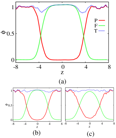
Figure 1: P-chain and f-chain density profiles showing the partitioning of the system into particle-based regions and field-based region in simulations of homopolymer solutions. Here P denotes the density profile of p-chains, F the density for f-chains, and T denotes their sum. For comparison, (b) and (c) shows the results for different choices of the number $S$ of p-f switch attempts per time step: (a) $S=500$ (default); (b) $S=50$; (c) $S=20$.

Figure 1 shows the density profiles of p-chains, f-chains, and their sum after equilibration of the system. As expected, p-chains aggregate near the borders at $z=-8$ and $z=8$, while f-chains mainly appear in the middle of the system. P-chains and f-chains are separated by interfaces with width about 2.5$R_{\mathrm{g}}$. The interface region can become even narrower if the tuning function is chosen sharper. However, due to the finite extension of chains, it must have a minimum width around $R_{\mathrm{g}}$. In principle, the total density should be independent of $\Delta\mu$, i.e., the summation of p-chain and f-chain density should be homogeneous. Indeed, in Figure (1), the total density in the p-chain region and f-chain region is almost constant apart from small statistical fluctuations. However, in the interface region, a small dip appears. Such dips are often observed in the interfacial regions of mixed resolution models fritsch ; poma ; HPF1 . In our case, it can partly be related to a discretization effect, as it becomes weaker if the number of grid points is increased. If necessary, it could be removed by introducing additional potentials in the interface region, following Ref. fritsch .

The efficiency of partitioning of course depends on the frequency of chain switch attempts. This is demonstrated in Figure (1) (b) and (c), where the number of attempts has been reduced from the “default” value $S=500$ (Figure  1 a) to $S=50$ and $S=20$ (Figure  1 b) and c). The interdiffusion of p- and f-chains competes with the chain switching, and therefore, the interfacial region broadens. This also reduces the density dip.

III.2 Interface broadening in an A/B polymer blend

Next we test our hybrid model on a more complex problem, the interdiffusion of miscible A/B polymers at an A/B interface. For comparison, we also run pure particle-based BD simulations (considered as the reference system) and pure LD calculations for the same system.

We consider systems containing $n_{\mathrm{A}}=5000$ A polymers and $n_{\mathrm{B}}=5000$ B polymers with the same chain length $N=20$. The melt is assumed to be compressible with $\kappa=10$, and A/B monomers are taken to be fully compatible, i.e., the incompatibility parameter $\chi$ (the Flory Huggins parameter) is set to $\chi=0$. Thus the nonbonded interactions are described by the Hamiltonian

$$\mathcal{H}_{\mathrm{I}}=\frac{n_{\mathrm{t}}\kappa}{2V}\int d\mathbf{r}\big{(}\phi_{\mathrm{A}}+\phi_{\mathrm{B}}-1\big{)}^{2}$$ (24)

where $n_{\mathrm{t}}=n_{\mathrm{A}}+n_{\mathrm{B}}$ is the total number of polymers in the system. This replaces (1) in Sec II, and Eq. (3) changes accordingly.

All simulations are implemented in three dimensional space with size $L_{\mathrm{x}}=L_{\mathrm{y}}=2$, and $L_{\mathrm{z}}=24$ decomposed into $n_{\mathrm{x}}\cdot n_{\mathrm{y}}\cdot n_{\mathrm{z}}=8\cdot 8\cdot 96$ uniform cells. To integrate the dynamical equations, we choose $\Delta t_{\mathrm{BD}}=5\cdot 10^{-4}t_{0}/N$, and $\Delta t_{\mathrm{LD}}=10^{-4}$ as in Sec III.1. Similarly, we also set $M=20$ and attempt 500 p-f switches are tried in each evolution step. Final statistical quantities are obtained by averaging over the results from 64 separate independent runs.

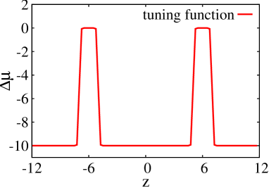
Figure 2: Profile of the tuning function, Eq. (25). This tuning function is adopted for both A polymer and B polymers.

Initially, we set the number of p-chains and f-chains for A and B polymers to equal values, i.e., $n_{\mathrm{Ap}}=n_{\mathrm{Af}}=n_{\mathrm{Bp}}=n_{\mathrm{Bf}}=2500$. The initial configuration for p-chains are generated from additional MC simulations leading to homogeneous density profiles along the $x$ and $y$ directions and sharp interfaces along $z$ direction. Therefore, in the following, we only consider the density profiles along the $z$ direction. For simplicity, the initial density profiles of f-chains are set such that $\phi_{\mathrm{Af}}(t=0)=\hat{\phi}_{\mathrm{Ap}}(t=0)$, and $\phi_{\mathrm{Bf}}(t=0)=\hat{\phi}_{\mathrm{Bp}}(t=0)$. At $t=0$, we thus have a strongly phase separated system with an A rich region near the boundaries (located at $z=-12$, and $z=12$), and a B rich region in the middle (See Fig. (4) for the initial density profile of A polymers $\phi_{\mathrm{A}}(t=0)$. The profiles of $\phi_{\mathrm{B}}(t=0)$ are not shown).

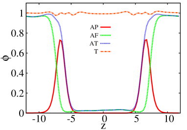
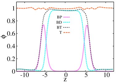
Figure 3: Density profiles for p-chains (AP), f-chains (AF), and the total of A polymers (AT) (a); density profiles for p-chains (BP), f-chains (BF), and the total of B polymers (BT) (b). Here T denotes the profile of total density of A and B polymers. These density profiles are extracted from the system at $t=0.1t_{0}$

We are interested in the A/B interface regions and want to keep the chain configuration properties there. Thus we need to resolve polymers as particles in the interface regions, while we can represent them by fields elsewhere. This can be done by choosing a tuning function for both A and B polymers such that it has large values in the interface regions and small values elsewhere. Specifically, we use

$$\Delta\mu=\frac{\mu_{\mathrm{a}}+\mu_{\mathrm{b}}}{2}+\frac{\mu_{\mathrm{a}}-\mu_{\mathrm{b}}}{2}\tan\bigg{[}\eta\Big{(}\Big{|}|z|-\frac{L_{\mathrm{z}}}{4}\Big{|}-\Delta\Big{)}\bigg{]}$$ (25)

where $\mu_{\mathrm{a}}=-10$, $\mu_{\mathrm{b}}=0$, $\eta=10$, $\Delta=1$ are parameters controlling the shape of $\Delta\mu$. The tuning function $\Delta\mu$ is plotted in Figure 2.

Figure 3 shows the density profiles at $t=0.1t_{0}$ of p-chains and f-chains for A and B polymers representing the successful partitioning of chains according to the tuning function. These one dimensional densities are obtained by averaging over the corresponding three dimensional densities in the $x$ and $y$ directions. In the early stage, $t\sim 0.1t_{0}$, the shape of the initial densities does not change very much, and most of the A polymers are still located near boundaries, while the B polymers are confined to a slab in the middle of the system. As expected, p-chains of both A and B polymers are mainly found in the interface regions (around $L_{\mathrm{z}}=-6$ and $L_{\mathrm{z}}=6$) with width about 2.5$R_{\mathrm{g}}$, and f-chains are distributed elsewhere. We find that that at $t\sim 0.1t_{0}$, the number of p-chains is roughly $n_{\mathrm{Ap}}\sim n_{\mathrm{Bp}}\sim 1000$, while the number of f-chains is $n_{\mathrm{Ap}}\sim n_{\mathrm{Bp}}\sim 4000$, i.e., about 20% of A polymers (and B polymers) are resolved by BD particles. Small dips can also be seen in the total density profiles similar to that in polymer solutions. With the presently chosen parameters, f-chains are not fully replaced by p-chains in the A/B interface regions, i.e., the maximum value of $\phi_{\mathrm{Ap}}$ and $\phi_{\mathrm{Bp}}$ does not reach the bulk value. One could easily adjust the parameters such that a wide slab in the interfacial region is filled by p-chains only. However, here we are interested in the interplay of particles and fields and its influence on the interdiffusion, which is why we keep the p-domains very narrow and f-chains can intrude.

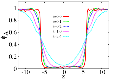
Figure 4: Density profiles for A polymers at different times from hybrid simulations. The times are measured in units of $t_{0}$.

Next we investigate the interfacial broadening process at early stages. This is done by monitoring the evolution of polymer densities. Since A polymer and B polymers are symmetric, we just focus on the properties of A polymers. Figure 4 shows the evolution of the A polymer density $\phi_{\mathrm{A}}(t)=\hat{\phi}_{\mathrm{Ap}}(t)+\phi_{\mathrm{Af}}(t)$. Starting from the initial sharp density profile, $\phi_{\mathrm{A}}(t)$ gradually becomes diffuse. At late times (not hown), $\phi_{\mathrm{A}}(t)$ approaches a uniform distribution with magnitude about 0.5.

To characterize the interfacial broadening more quantitatively, we introduce a quantity $W$ measuring the interfacial width, and monitor $W$ as a function of time. The “interfacial width” $W$ is simply defined as the inverse of the maximum slope of the density profile. We do not renormalize it to the “bulk densities”, as the latter are changing with time and are thus not well defined. Figure 5 plots the evolution of width $W(t)$ obtained with our hybrid method, and compares with with data from pure particle-based BD simulations and from pure field-based LD simulations. The initial densities in the pure LD calculations is set the same as that in the pure BD simulations. Except for early times ($t<0.1t_{0}$), where deviations are observed due to the finite interfacial width effect, the curves for the hybrid model, the pure BD simulations and pure LD theory are rather well described by a scaling relation broaden1 ; broaden2 ; broaden3 $W\sim t^{a}$ with exponent $a\sim 0.45$.

The simulation data obtained with the hybrid model are in excellent agreement with those obtained from the fully fine-grained BD model. In contrast, the data from the LD simulations show deviations at early times. These presumably reflect the importance of density fluctuations in the interface region, which are neglected in the coarse-grained LD approach. This problem can be avoided by resorting to the hybrid description.

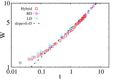
Figure 5: Evolution of A/B interfacial width $W$ as a function of time (in units $t_{0}$) according to different models as indicated. The dashed line is plotted to guide eyes and it indicates a power law $W(t)\sim t^{a}$ with $a\simeq 0.45$. The size of error bar for the data obtained from hybrid simulations is similar to that from pure BD simulations (not shown).

IV Summary and remarks

In this work, we have developed a hybrid scheme that dynamically couples a particle-based description of polymers to a field-based description in an adaptive resolution sense, where polymers can switch between different resolutions on the fly. The resolution switch is controlled by a predefined tuning function through a Monte Carlo criterion. In order to capture the dynamic behavior, we use Brownian dynamics at the particle level, and a local density functional theory at the field level. The hybrid scheme was explained in detail at the example of a polymer solution, and then tested in simulations of a more complex problem, the interface broadening in a polymer A/B blend.

In the applications presented here, the tuning function was kept constant throughout the simulation. The geometric partitioning into particle and field domains was thus pre-defined prior to the simulation. However, the partitioning has no physical meaning, and the tuning function can be chosen at will, which means that it can also be adjusted to the configuration during the simulation. For example, in a large-scale simulation of A/B interfaces in immiscible polymer blends, capillary undulations of the interface must be taken into account. The fine-grained p-domain should thus be able to follow the local position of the interface. This could be done, e.g., by coupling the tuning function to the local concentration difference of A and B monomers, or to concentration gradients.

We should note apart from LD, a number of other dynamic density functional theories (DDFTs) have been proposed for dynamic studies of polymer systems LD2 ; fluctuation_dynamics . Unfortunately, in contrast to simple liquids simple_DFT1 ; simple_DFT2 ; simple_DFT3 ; simple_DFT4 ; simple_DFT5 , it is not possible to derive d DDFT for polymers which is based on densities only and fully equivalent to the BD description BD_to_DDFT1 ; BD_to_DDFT2 . Therefore, DDFTs for polymers always rely on approximations and represent different aspects of the polymer motion. The local DDFT used here (the LD method) focusses on individual monomers and disregards the effect of chain connectivity. Other DDFTs such that Debye dynamics and external potential dynamics LD2 account for the chain connectivity and focus on the collective motion of monomers in a chain. In a recent work BD_and_DDFT , we have compared several DDFT approaches with BD simulations, and shown that the LD scheme reproduces the interfacial evolution in A/B homopolymer or the kinetics of microscopic phase separation in A:B diblock copolymer melts fairly accurately. However, in other situations, the kinetic pathways of structure formation in DDFT simulations may depend on the choice of the DDFT LB_DSCF ; LB_EPD . Therefore, to complete the hybrid modelling scheme, we also tested models where the f-chains are propagated according to DDFT equations that account for chain connectivity, e.g., Debye dynamics. Unfortunately, we found that such schemes tend to suffer from a flow imbalance in the f-p interfacial region. As a result, the overall density is no longer constant, an accumulation of chains is observed in the p- or f-domain, and corrections have to be applied. A detailed analysis will be published elsewhere.

Another important extension in future work will be to add inertia and account for momentum conservation. At the coarse-grained particle level, this is easily done by switching from Brownian Dynamics to Molecular Dynamics, possibly in combination with a momentum-conserving thermostat that restores friction effects agur . At the field level, one option is to use a recently developed scheme that couples DDFT with Lattice Boltzmann simulations LB_DSCF ; LB_EPD .

Hybrid particle-field schemes can be useful in a variety of contexts: Firstly, they can be used to implement proper boundary conditions in field-based simulations HPF2 . This is particularly important in situations where complex surfaces or interfaces critically influence the relevant properties of a material. Examples are liquid crystal cells where surfaces define the orientation of the director, or composite materials with polymer-coated filler particles. Secondly, they can be used for particle- based simulations of polymeric systems with open boundary conditions. The main purpose of the field domain is then to provide a realistic environment for the system of interest and act as polymer reservoir. We believe that our HPF approach and suitable refinements and extensions will provide a convenient and practical tool for such applications.

ACKNOWLEDGMENTS

We wish to thank H. Behringer and T. Raasch for useful discussions. Financial support from the German Science Foundation (DFG) within project C1 in SFB TRR 146 is gratefully acknowledged. Simulations have been carried out on the supercomputer Mogon at Johannes Gutenberg University Mainz (hpc.uni-mainz.de).

References

- (1) J. Baschnagel, K. Binder, P. Doruker, A. A. Gusev, O. Hahn, K. Kremer, W. L. Mattice, F. Müller-Plathe, M. Murat, W. Paul, S. Santos, U. W. Suter, and V. Tries, Adv. Polym. Sci., 2000, 152, 41.
- (2) M. Praprotnik, L. D. Site, and K. Kremer, Annu. Rev. Phys. Chem., 2008, 59, 545.
- (3) M. Praprotnik, L. Delle Site, and K. Kremer, J. Chem. Phys., 2005, 123, 224106.
- (4) B. Ensing, S.O. Nielsen, P.B. Moore, M.L. Klein, and M. Parrinello, J. Chem. Theory Comput., 2007, 3, 1100.
- (5) A. Heyden and D.G. Truhlar, J. Chem. Theory Comput., 2008, 4, 217.
- (6) M. Praprotnik, L. Delle Site, and K. Kremer, Phys. Rev. E., 2006, 73, 066701.
- (7) A.B. Poma and L. Delle Site, Phys. Rev. Lett., 2010, 104, 250201.
- (8) A.B. Poma and L. Delle Site, Phys. Chem. Chem. Phys., 2011, 13, 10510.
- (9) S. Fritsch, S. Poblete, C. Junghans, G. Ciccotti, L. D. Site, and K. Kremer, Phys. Rev. Lett., 2012, 108, 170602.
- (10) R. Potestio, S. Fritsch, P. Español, R. Delgado-Buscalioni, K. Kremer, R. Everaers, and D. Donadio, Phys. Rev. Lett., 2013, 110, 108301.
- (11) G De Fabritiis, R. Delgado-Buscalioni, and P. V. Coveney, Phys. Rev. Lett., 2006, 97, 134501.
- (12) R. Delgado-Buscalioni and G De Fabritiis, Phys. Rev. E, 2007, 76, 036709.
- (13) R. Delgado-Buscalioni, K. Kremer, and M. Praprotnik, J. Chem. Phys., 2008, 128, 114110.
- (14) R. Delgado-Buscalioni, K. Kremer, and M. Praprotnik, J. Chem. Phys., 2009, 131, 244107.
- (15) I. Korotkin, S. Karabasov, D. Nerukh, A. Markesteijn, A. Scukins, V. Farafonov, and E. Pavlov, J. Chem. Phys., 2015, 143, 014110.
- (16) S. Qi, H. Behringer, and F. Schmid, New J. Phys., 2013, 15, 125009.
- (17) S. Qi, H. Behringer, T. Raasch, and F. Schmid, Eur. Phys. J. Special Topics, 2016, 25, 1527.
- (18) M. J. Field, P. A. Bash, and M. Karplus, J. Comp. Chem., 1990, 11, 700.
- (19) A. Donev, J. B. Bell, A. L. Garcia, and B. J. Alder, Multiscale Model. Simul., 2010, 8, 871.
- (20) L. Miao, H. Guo, and M. J. Zuckermann, Macromolecules, 1996, 29, 2289.
- (21) M. G. Saphiannikova, V. A. Pryamitsyn, and T. Cosgrove, Macromolecules, 1998, 31, 6662.
- (22) S. W. Sides, B. J. Kim, E. J. Kramer, and G. H. Fredrickson, Phys. Rev. Lett., 2006, 96, 250601.
- (23) V. Ganesan and V. Pryamitsyn, J. Chem. Phys., 2003, 118, 4345.
- (24) B. Narayanan, V. A. Pryamitsyn, and V. Ganesan, Macromolecules, 2004, 37, 10180.
- (25) N. D. Petsev, L. G. Leal, and M. S. Shell, J. Chem. Phys., 2015, 142, 044101.
- (26) P. M. Kulkami, C.-C. Fu, M. S. Shell, and L. G. Leal, J. Chem. Phys., 2013, 138, 234105.
- (27) P. Español and M. Revenga, Phys. Rev. E, 2003, 67, 026705.
- (28) U. Alekseeva, R. G. Winkler, and G. Sutmann, J. Comput. Phys., 2016, 314, 14.
- (29) G. Milano and T. Kawakatsu, J. Chem. Phys., 2009, 130, 214106.
- (30) G. Milano and T. Kawakatsu, J. Chem. Phys., 2010, 133, 214102.
- (31) G. Milano, T. Kawakatsu, and A. de Nicola, Phys. Biol., 2013, 10, 045007.
- (32) M. Laradji, H. Guo, and M.J. Zuckermann, Phys. Rev. E., 1994, 49, 3199.
- (33) G. Besold, H. Guo, and M.J. Zuckermann, J. Poly. Sci. Part B: Polym. Phys., 2000, 38, 1053.
- (34) M. Müller and G.D. Smith, J. Polym. Sci.: Part B: Polym. Phys., 2005, 43, 934.
- (35) K. Ch Daoulas and M. Müller, J. Chem. Phys., 2006, 125 184904.
- (36) S. F. Edwards, Proc. Phys. Soc., 1965, 85, 613.
- (37) P. G. de Gennes, Rep. Prog. Phys., 1969, 32, 187.
- (38) S. F. Edwards, Proc. Phys. Soc., 1966, 88, 265.
- (39) K. Freed, Renormalization Group Theory of Macromolecules (New York: Wiley, 1987).
- (40) K.M. Hong, J. Noolandi, Macromolecules, 1981, 14, 727.
- (41) F. Schmid, J. Phys. Condens. Matter, 1998, 10, 8105.
- (42) G. H. Fredrickson, The Equilibrium Theory of Inhomogeneous Polymers (Oxford University Press, Oxford, 2006).
- (43) H. D. Ceniceros and G. H. Fredrickson, Multiscale Model. Simul., 2004, 2, 452.
- (44) M. Müller, F. Schmid, Adv. Polym. Sci., 2005, 185, 1.
- (45) P. Stasiak, M. Matsen, Eur. Phys. J. E, 2011, 34, 110.
- (46) M. Doi and S. F. Edwards, The Theory of Polymer Dynamics (Oxford University Press, 1999).
- (47) S. Zhang, S. Qi, L. I. Klushin, A. M. Skvortsov, D. Yan, and F. Schmid, J. Chem. Phys., 2017, 147, 064902.
- (48) F. A. Detcheverry, H. Kang, K. C. Daoulas, M. Müller, P. F. Nealey, and J. J. de Pablo, Macromolecules, 2008, 41, 4989.
- (49) S. Qi, L. I. Klushin, A. M. Skvortsov, A. A. Polotsky, and F. Schmid, Macromolecules, 2015, 48, 3775.
- (50) S. Qi, L. I. Klushin, A. M. Skvortsov, and F. Schmid, Macromolecules, 2016, 49, 9665.
- (51) C.K. Birdsall and D. Fuss, J. Comput. Phys., 1997, 135, 141.
- (52) J. G. E. M. Fraaije, B. A. C. van Vlimmeren, N. M. Maurits, M. Postma, O. A. Evers, C. Hoffmann, P. Altevogt, and G. Goldbeck-Wood, J. Chem. Phys., 1997, 106, 4260.
- (53) N. M. Maurits and J. G. E. M. Fraaije, J. Chem. Phys., 1997, 107, 5879.
- (54) T. Uneyama, J. Chem. Phys., 2007, 126, 114902.
- (55) W. H. Press, S. A. Teukolsky, W. T. Vetterling, B. P. Flannery, Numerical Recipes in C: The Art of Scientific Computing, 2nd ed.; (Cambridge University Press, 1992).
- (56) D. P. Landau and K. Binder, A Guide to Monte Carlo Simulations in Statistical Physics, Second Edition, (Cambridge Press, UK, 2000)
- (57) D. Frenkel and B. Smit, Understanding Molecular Simulation from Algorithms to Applications, (Academic Press, UK, 2002)
- (58) S. Fritsch, S. Poblete, C. Junghans, G. Ciccotti, L. Delle Site, K. Kremer, Phys. Rev. Lett., 2012, 108, 170602.
- (59) A.B. Poma, L. Delle Site, Phys. Rev. Lett., 2010, 104, 250201.
- (60) S. Q. Wang and Q. Shi, Macromolecules, 1993, 26, 1091.
- (61) C. Yeung and A.-C. Shi, Macromolecules, 1999, 32, 3637.
- (62) S. Qi, X. Zhang, and D. Yan, J. Chem. Phys., 2010, 132, 064903.
- (63) D. S. Dean, J. Phys. A: Math. Gen., 1996, 29, L613.
- (64) H. Frusawa and R. Hayakawa, J. Phys. A: Math. Gen., 2000, 33, L155.
- (65) U. M. B. Marconi and P Tarazona, J. Chem. Phys., 1999, 110, 8032.
- (66) R. Evans and A. J. Archer, J. Chem. Phys., 2004, 37, 9325.
- (67) A. J. Archer and M. Rauscher, J. Phys. A: Math. Gen., 2004, 37, 9325.
- (68) G. H. Fredrickson and H. Orland, J. Chem. Phys., 2014, 140, 084902.
- (69) D. J. Grzetic, R. A. Wickham, and A.-C. Shi, J. Chem. Phys., 2014, 140, 244907.
- (70) S. Qi and F. Schmid, “Dynamic density functional theories for inhomogeneous polymer systems compared to Brownian dynamics simulatons”, Preprint.
- (71) L. Zhang, G. J. A. Sevink, and F. Schmid, Macromolecules, 2011, 44, 9434.
- (72) J. Heuser, G. J. A. Sevink, and F. Schmid, Macromolecules, 2017, 50, 4474.
- (73) G. J. A. Sevink, F. Schmid, T. Kawakatsu, G. Milano, Soft Matter, 2017, 13, 1594.