Visualizing and Improving Scattering Networks

Abstract

Scattering Transforms (or ScatterNets) introduced by Mallat in [1] are a promising start into creating a well-defined feature extractor to use for pattern recognition and image classification tasks. They are of particular interest due to their architectural similarity to Convolutional Neural Networks (CNNs), while requiring no parameter learning and still performing very well (particularly in constrained classification tasks).

In this paper we visualize what the deeper layers of a ScatterNet are sensitive to using a ‘DeScatterNet’. We show that the higher orders of ScatterNets are sensitive to complex, edge-like patterns (checker-boards and rippled edges). These complex patterns may be useful for texture classification, but are quite dissimilar from the patterns visualized in second and third layers of Convolutional Neural Networks (CNNs) - the current state of the art Image Classifiers. We propose that this may be the source of the current gaps in performance between ScatterNets and CNNs (83% vs 93% on CIFAR-10 for ScatterNet+SVM vs ResNet). We then use these visualization tools to propose possible enhancements to the ScatterNet design, which show they have the power to extract features more closely resembling CNNs, while still being well-defined and having the invariance properties fundamental to ScatterNets.

Index Terms—  ScatterNets, DeScatterNets, Scattering Network, Convolutional Neural Network, Visualization, $\mathrm{DT}{\mathbb{C}}\mathrm{WT}$

1 Introduction

Scattering transforms, or ScatterNets, have recently gained much attention and use due to their ability to extract generic and descriptive features in well defined way. They can be used as unsupervised feature extractors for image classification [2, 3, 4, 5] and texture classification [6], or in combination with supervised methods such as Convolutional Neural Networks (CNNs) to make the latter learn quicker, and in a more stable way [7].

ScatterNets have been shown to perform very well as image classifiers. In particular, they can outperform CNNs for classification tasks with reduced training set sizes, e.g. in CIFAR-10 and CIFAR-100 (Table 6 from [7] and Table 4 from [4]). They are also near state-of-the-art for Texture Discrimination tasks (Tables 1–3 from [6]). Despite this, there still exists a considerable gap between them and CNNs on challenges like CIFAR-10 with the full training set ($~{}83\%$ vs. $~{}93\%$). Even considering the benefits of ScatterNets, this gap must be addressed.

We first revise the operations that form a ScatterNet in Section 2. We then introduce our DeScatterNet (Section 3), and show how we can use it to examine the layers of ScatterNets (using a similar technique to the CNN visualization in [8]). We use this analysis tool to highlight what patterns a ScatterNet is sensitive to (Section 4), showing that they are very different from what their CNN counterparts are sensitive to, and possibly less useful for discriminative tasks.

We use these observations to propose an architectural change to ScatterNets, which have not changed much since their inception in [1]. Two changes of note however are the work of Sifre and Mallat in [6], and the work of Singh and Kingsbury in [4]. Sifre and Mallat introduced Rotationally Invariant ScatterNets which took ScatterNets in a new direction, as the architecture now included filtering across the wavelet orientations (albeit with heavy restrictions on the fitlers used). Singh and Kingsbury achieved improvements in performance in a Scattering system using the spatially implementable $\mathrm{DT}{\mathbb{C}}\mathrm{WT}$ [9] wavelets instead of the Fourier Transform (FFT) based Morlet previously used.

We build on these two systems, showing that with carefully designed complex filters applied across the complex spatial coefficients of a 2-D $\mathrm{DT}{\mathbb{C}}\mathrm{WT}$, we can build filters that are sensitive to more recognizable shapes like those commonly seen in CNNs, such as corners and curves (Section 5).

2 The Scattering Transform

The Scattering Transform, or ScatterNet, is a cascade of complex wavelet transforms and modulus non-linearities (throwing away the phase of the complex wavelet coefficients). At a chosen scale, averaging filters provide invariance to nuisance variations such as shift and deformation (and potentially rotations). Due to the non-expansive nature of the wavelet transform and the modulus operation, this transform is stable to deformations.

Typical implementations of the ScatterNet are limited to two ‘orders’ (equivalent to layers in a CNN) [3, 4, 7]. In addition to scattering order, we also have the scale of invariance, $J$. This is the number of band-pass coefficients output from a wavelet filter bank (FB), and defines the cut-off frequency for the final low-pass output: $2^{-J}\frac{f_{s}}{2}$ ($f_{s}$ is the sampling frequency of the signal). Finally, we call the number of oriented wavelet coefficients used $L$. These are the three main hyper-parameters of the scattering transform and must be set ahead of time. We describe a system with scale parameter $J=4$, order $m=2$ and with $L=6$ orientations ($L$ is fixed to 6 for the $\mathrm{DT}{\mathbb{C}}\mathrm{WT}$ but is flexible for the FFT based Morlet wavelets).

Consider an input signal $x(\bm{u}),\bm{u}\in{\mathbb{R}}^{2}$. The zeroth order scatter coefficient is the lowpass output of a $J$ level FB:

$$S_{0}x(\bm{u})\triangleq(x\ast\phi_{J})(\bm{u})$$ (1)

This is invariant to translations of up to $2^{J}$ pixels. In exchange for gaining invariance, the $S_{0}$ coefficients have lost a lot of information (contained in the rest of the frequency space). The remaining energy of $x$ is contained within the first order wavelet coefficients:

$$W_{1}x(\bm{u},j_{1},\theta_{1})\triangleq x\ast\psi_{j_{1},\theta_{1}}$$ (2)

for $j_{1}\in\{1,2,\ldots,J\},\theta_{1}\in\{1,2,\ldots,L\}$. We will want to retain this information in these coefficients to build a useful classifier.

Let us call the set of available scales and orientations $\Lambda_{1}$ and use $\lambda_{1}$ to index it. For both Morlet and $\mathrm{DT}{\mathbb{C}}\mathrm{WT}$ implementations, $\psi$ is complex-valued, i.e., $\psi=\psi^{r}+j\psi^{i}$ with $\psi_{r}$ and $\psi_{i}$ forming a Hilbert Pair, resulting in an analytic $\psi$. This analyticity provides a source of invariance — small input shifts in $x$ result in a phase rotation (but little magnitude change) of the complex wavelet coefficients.

Taking the magnitude of $W_{1}$ gives us the first order propagated signals:

$$U_{1}x(\bm{u},\lambda_{1})\triangleq|x\ast\psi_{\lambda}|=\sqrt{(x\ast\psi^{r}_{\lambda_{1}})^{2}+(x\ast\psi^{i}_{\lambda_{1}})^{2}}$$ (3)

The first order scattering coefficient makes $U_{1}$ invariant up to our scale $J$ by averaging it:

$$S_{1}x(\bm{u},\lambda_{1})\triangleq|x\ast\psi_{\lambda}|\ast\phi_{J}$$ (4)

If we define $U_{0}\triangleq x$, then we can iteratively define:

$$W_{m} = U_{m-1}\ast\psi_{\lambda_{m}}$$ (5)

$$U_{m} = |W_{m}|$$ (6)

$$S_{m} = U_{m}\ast\phi_{J}$$ (7)

We repeat this for higher orders, although previous work shows that, for natural images, we get diminishing returns after $m=2$. The output of our ScatterNet is then:

$$Sx=\{S_{0}x,S_{1}x,S_{2}x\}$$ (8)

2.1 Scattering Color Images

A wavelet transform like the $\mathrm{DT}{\mathbb{C}}\mathrm{WT}$ accepts single channel input, while we often work on RGB images. This leaves us with a choice. We can either:

1. Apply the wavelet transform (and the subsequent scattering operations) on each channel independently. This would triple the output size to $3C$.

2. Define a frequency threshold below which we keep color information, and above which, we combine the three channels into a single luminance channel.

The second option uses the well known fact that the human eye is far less sensitive to higher spatial frequencies in color channels than in luminance channels. This also fits in with the first layer filters seen in the well known Convolutional Neural Network, AlexNet. Roughly one half of the filters were low frequency color ‘blobs’, while the other half were higher frequency, grayscale, oriented wavelets.

For this reason, we choose the second option for the architecture described in this paper. We keep the 3 color channels in our $S_{0}$ coefficients, but work only on grayscale for high orders (the $S_{0}$ coefficients are the lowpass bands of a J-scale wavelet transform, so we have effectively chosen a color cut-off frequency of $2^{-J}\frac{f_{s}}{2}$).

For example, consider an RGB input image $x$ of size $64\times 64\times 3$. The scattering transform we have described with parameters $J=4$ and $m=2$ would then have the following coefficients:

$$S_{0} : (64\times 2^{-J})\times(64\times 2^{-J})\times 3=4\times 4\times 3$$

$$S_{1} : 4\times 4\times(LJ)=4\times 4\times 24$$

$$S_{2} : 4\times 4\times\left(\frac{1}{2}L^{2}J(J-1)\right)=4\times 4\times 216$$

$$S : 4\times 4\times(216+24+3)=4\times 4\times 243$$

3 The Inverse Network

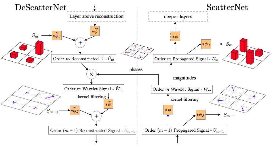
Fig. 1: A DeScattering layer (left) attached to a Scattering layer (right). We are using the same convention as [8] Figure 1 - the input signal starts in the bottom right hand corner, passes forwards through the ScatterNet (up the right half), and then is reconstructed in the DeScatterNet (downwards on the left half). The DeScattering layer will reconstruct an approximate version of the previous order’s propagated signal. The $2\times 2$ grids shown around the image are either Argand diagrams representing the magnitude and phase of small regions of complex (De)ScatterNet coefficients, or bar charts showing the magnitude of the real (De)ScatterNet coefficients (after applying the modulus non-linearity). For reconstruction, we need to save the discarded phase information and reintroduce it by multiplying it with the reconstructed magnitudes.

We now introduce our inverse scattering network. This allows us to back project scattering coefficients to the image plane; it is inspired by the DeconvNet used by Zeiler and Fergus in [8] to look into the deeper layers of CNNs.

We emphasize that instead of thinking about perfectly reconstructing $x$ from $S\in{\mathbb{R}}^{H^{\prime}\times W^{\prime}\times C}$, we want to see what signal/pattern in the input image caused a large activation in each channel. This gives us a good idea of what each output channel is sensitive to, or what it extracts from the input. Note that we do not use any of the log normalization layers described in [3, 4].

3.1 Inverting the Low-Pass Filtering

Going from the $U$ coefficients to the $S$ coefficients involved convolving by a low pass filter, $\phi_{J}$ followed by decimation to make the output $(H\times 2^{-J})\times(W\times 2^{-J})$. $\phi_{J}$ is a purely real filter, and we can ‘invert’ this operation by interpolating $S$ to the same spatial size as $U$ and convolving with the mirror image of $\phi_{J}$, $\widetilde{\phi}_{J}$ (this is equivalent to the transpose convolution described in [8]).

$$\hat{S}_{m}=S_{m}\ast\widetilde{\phi}_{J}$$ (9)

This will not recover $U$ as it was on the forward pass, but will recover all the information in $U$ that caused a strong response in $S$.

3.2 Inverting the Magnitude Operation

In the same vein as [8], we face a difficult task in inverting the non-linearity in our system. We lend inspiration from the switches introduced in the DeconvNet; the switches in a DeconvNet save the location of maximal activations so that on the backwards pass activation layers could be unpooled trivially. We do an equivalent operation by saving the phase of the complex activations. On the backwards pass we reinsert the phase to give our recovered $W$.

$$\hat{W}_{m}=\hat{U}_{m}e^{j\theta_{m}}$$ (10)

3.3 Inverting the Wavelet Decomposition

Using the $\mathrm{DT}{\mathbb{C}}\mathrm{WT}$ makes inverting the wavelet transform simple, as we can simply feed the coefficients through the synthesis filter banks to regenerate the signal. For complex $\psi$, this is convolving with the conjugate transpose $\widetilde{\psi}$:

$$\hat{U}_{m-1} = \hat{S}_{m-1}+\hat{W}_{m}$$ (11)

$$= S_{m-1}\ast\widetilde{\phi}_{J}+\sum_{j,\theta}W_{m}(\bm{u},j,\theta)\ast\widetilde{\psi}_{j,\theta}$$

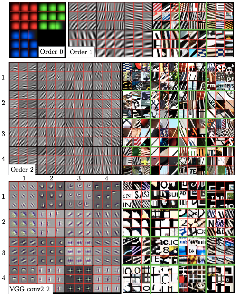
Fig. 2: Visualization of a random subset of features from $S_{0}$ (all 3), $S_{1}$ (6 from the 24) and $S_{2}$ (16 from the 240) scattering outputs. We record the top 9 activations for the chosen features and project them back to the pixel space. We show them alongside the input image patches which caused the large activations. We also include reconstructions from layer conv2_2 of VGG Net [10](a popular CNN, often used for feature extraction) for reference — here we display 16 of the 128 channels. The VGG reconstructions were made with a CNN DeconvNet based on [8]. Image best viewed digitally.

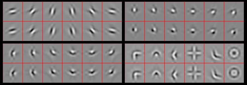
Fig. 3: Shapes possible by filtering across the wavelet orientations with complex coefficients. All shapes are shown in pairs: the top image is reconstructed from a purely real output, and the bottom image from a purely imaginary output. These ‘real’ and ‘imaginary’ shapes are nearly orthogonal in the pixel space (normalized dot product $<0.01$ for all but the doughnut shape in the bottom right, which has $0.15$) but produce the same $U^{\prime}$, something that would not be possible without the complex filters of a ScatterNet. Top left - reconstructions from $U_{1}$ (i.e. no cross-orientation filtering). Top right- reconstructions from $U_{1}^{\prime}$ using a $1\times 1\times 12$ Morlet Wavelet, similar to what was done in the ‘Roto-Translation’ ScatterNet described in [6, 3]. Bottom left - reconstructions from $U_{1}^{\prime}$ made with a more general $1\times 1\times 12$ filter, described in Equation 14. Bottom right - some reconstructions possible by filtering a general $3\times 3\times 12$ filter.

4 Visualization with Inverse Scattering

To examine our ScatterNet, we scatter all of the images from ImageNet’s validation set and record the top 9 images which most highly activate each of the $C$ channels in the ScatterNet. This is the identification phase (in which no inverse scattering is performed).

Then, in the reconstruction phase, we load in the $9\times C$ images, and scatter them one by one. We take the resulting $4\times 4\times 243$ output vector and mask all but a single value in the channel we are currently examining.

This 1-sparse tensor is then presented to the inverse scattering network from Figure 1 and projected back to the image space. Some results of this are shown in Figure 2. This figure shows reconstructed features from the layers of a ScatterNet. For a given output channel, we show the top 9 activations projected independently to pixel space. For the first and second order coefficients, we also show the patch of pixels in the input image which cause this large output. We display activations from various scales (increasing from first row to last row), and random orientations in these scales.

The order 1 scattering (labelled with ‘Order 1’ in Figure 2) coefficients look quite similar to the first layer filters from the well known AlexNet CNN [11]. This is not too surprising, as the first order scattering coefficients are simply a wavelet transform followed by average pooling. They are responding to images with strong edges aligned with the wavelet orientation.

The second order coefficients (labelled with ‘Order 2’ in Figure 2) appear very similar to the order 1 coefficients at first glance. They too are sensitive to edge-like features, and some of them (e.g. third row, third column and fourth row, second column) are mostly just that. These are features that have the same oriented wavelet applied at both the first and second order. Others, such as the 9 in the first row, first column, and first row, fourth column are more sensitive to checker-board like patterns. Indeed, these are activations where the orientation of the wavelet for the first and second order scattering were far from each other (15^∘ and 105^∘ for the first row, first column and 105^∘ and 45^∘ for the first row, fourth column).

For comparison, we include reconstructions from the second layer of the well-known VGG CNN (labelled with ‘VGG conv2_2’, in Figure 2). These were made with a DeconvNet, following the same method as [8]. Note that while some of the features are edge-like, we also see higher order shapes like corners, crosses and curves.

5 Corners, Crosses and Curves

These reconstructions show that the features extracted from ScatterNets vary significantly from those learned in CNNs after the first order. In many respects, the features extracted from a CNN like VGGNet look preferable for use as part of a classification system.

[6] and [3] introduced the idea of a ‘Roto-Translation’ ScatterNet. Invariance to rotation could be made by applying averaging (and bandpass) filters across the $L$ orientations from the wavelet transform before applying the complex modulus. Momentarily ignoring the form of the filters they apply, referring to them as $F_{k}\in{\mathbb{C}}^{L}$, we can think of this stage as stacking the $L$ outputs of a complex wavelet transform on top of each other, and convolving these filters $F_{k}$ over all spatial locations of the wavelet coefficients $W_{m}x$ (this is equivalent to how filters in a CNN are fully connected in depth):

$$V_{m}x(\bm{u},j,k)=W_{m}x\ast F_{k}=\sum_{\theta}W_{m}x(\bm{u},j,\theta)F_{k}(\theta)$$ (12)

We then take the modulus of these complex outputs to make a second propagated signal:

$$U_{m}^{\prime}x\triangleq|V_{m}x|=|W_{m}x\ast F_{k}|=|U_{m-1}x\ast\psi_{\lambda_{m}}\ast F_{k}|$$ (13)

We present a variation on this idea, by filtering with a more general $F\in{\mathbb{C}}^{H\times W\times 12}$. We use $F$ of length 12 rather than 6, as we use the $L=6$ orientations and their complex conjugates; each wavelet is a 30^∘ rotation of the previous, so with 12 rotations, we can cover the full $360{{}^{\circ}}$.

Figure 3 shows some reconstructions from these $V$ coefficients. Each of the four quadrants show reconstructions from a different class of ScatterNet layer. All shapes are shown in real and imaginary Hilbert-like pairs; the top images in each quadrant are reconstructed from a purely real $V$, while the bottom inputs are reconstructed from a purely imaginary $V$. This shows one level of invariance of these filters, as after taking the complex magnitude, both the top and the bottom shape will activate the filter with the same strength. In comparison, for the purely real filters of a CNN, the top shape would cause a large output, and the bottom shape would cause near 0 activity (they are nearly orthogonal to each other).

In the top left, we display the 6 wavelet filters for reference (these were reconstructed from $U_{1}$, not $V_{1}$). In the top right of the figure we see some of the shapes made by using the $F$’s from the Roto-Translation ScatterNet [6, 3]. The bottom left is where we present some of our novel kernels. These are simple corner-like shapes made by filtering with ${F\in{\mathbb{C}}^{1\times 1\times 12}}$

$$F=[1,j,j,1,0,0,0,0,0,0,0,0]$$ (14)

The six orientations are made by rolling the coefficients in $F$ along one sample (i.e. $[0,1,j,j,1,0,\ldots]$, $[0,0,1,j,j,1,0,\ldots]$, $[0,0,0,1,j,j,1,0,\ldots]$ …). Coefficients roll back around (like circular convolution) when they reach the end.

Finally, in the bottom right we see shapes made by ${F\in{\mathbb{C}}^{3\times 3\times 12}}$. Note that with the exception of the ring-like shape which has 12 non-zero coefficients, all of these shapes were reconstructed with $F$’s that have 4 to 8 non-zero coefficients of a possible 64. These shapes are now beginning to more closely resemble the more complex shapes seen in the middle stages of CNNs.

6 Discussion

This paper presents a way to investigate what the higher orders of a ScatterNet are responding to - the DeScatterNet described in Section 3. Using this, we have shown that the second ‘layer’ of a ScatterNet responds strongly to patterns that are very dissimilar to those that highly activate the second layer of a CNN. As well as being dissimilar to CNNs, visual inspection of the ScatterNet’s patterns reveal that they may be less useful for discriminative tasks, and we believe this may be causing the current gaps in state-of-the-art performance between the two.

We have presented an architectural change to ScatterNets that can make it sensitive to more recognizable shapes. We believe that using this new layer is how we can start to close the gap, making more generic and descriptive ScatterNets while keeping control of their desirable properties.

A future paper will include classifier results for these new filters.

References

- [1] Stéphane Mallat, “Group Invariant Scattering,” Communications on Pure and Applied Mathematics, vol. 65, no. 10, pp. 1331–1398, Oct. 2012.
- [2] J. Bruna and S. Mallat, “Invariant Scattering Convolution Networks,” IEEE Transactions on Pattern Analysis and Machine Intelligence, vol. 35, no. 8, pp. 1872–1886, Aug. 2013.
- [3] Edouard Oyallon and Stephane Mallat, “Deep Roto-Translation Scattering for Object Classification,” 2015, pp. 2865–2873.
- [4] Amarjot Singh and Nick Kingsbury, “Dual-Tree Wavelet Scattering Network with Parametric Log Transformation for Object Classification,” arXiv:1702.03267 [cs], Feb. 2017.
- [5] Amarjot Singh and Nick Kingsbury, “Multi-Resolution Dual-Tree Wavelet Scattering Network for Signal Classification,” arXiv:1702.03345 [cs], Feb. 2017.
- [6] L. Sifre and S. Mallat, “Rotation, Scaling and Deformation Invariant Scattering for Texture Discrimination,” in 2013 IEEE Conference on Computer Vision and Pattern Recognition (CVPR), June 2013, pp. 1233–1240.
- [7] Edouard Oyallon, Eugene Belilovsky, and Sergey Zagoruyko, “Scaling the Scattering Transform: Deep Hybrid Networks,” arXiv:1703.08961 [cs], Mar. 2017.
- [8] Matthew D. Zeiler and Rob Fergus, “Visualizing and Understanding Convolutional Networks,” in Computer Vision – ECCV 2014, Sept. 2014, pp. 818–833.
- [9] N. Kingsbury, “Complex wavelets for shift invariant analysis and filtering of signals,” Applied and Computational Harmonic Analysis, vol. 10, no. 3, pp. 234–253, May 2001.
- [10] Karen Simonyan and Andrew Zisserman, “Very Deep Convolutional Networks for Large-Scale Image Recognition,” arXiv:1409.1556 [cs], Sept. 2014.
- [11] Alex Krizhevsky, Ilya Sutskever, and Geoffrey E. Hinton, “ImageNet Classification with Deep Convolutional Neural Networks,” in NIPS. 2012, pp. 1097–1105, Curran Associates, Inc.