A Unification and Generalization of Exact Distributed First Order Methods

Abstract

Recently, there has been significant progress in the development of distributed first order methods. (At least) two different types of methods, designed from very different perspectives, have been proposed that achieve both exact and linear convergence when a constant step size is used – a favorable feature that was not achievable by most prior methods. In this paper, we unify, generalize, and improve convergence speed of these exact distributed first order methods. We first carry out a novel unifying analysis that sheds light on how the different existing methods compare. The analysis reveals that a major difference between the methods is on how a past dual gradient of an associated augmented Lagrangian dual function is weighted. We then capitalize on the insights from the analysis to derive a novel method – with a tuned past gradient weighting – that improves upon the existing methods. We establish for the proposed generalized method global R-linear convergence rate under strongly convex costs with Lipschitz continuous gradients.

I Introduction

Context and motivation. Distributed optimization methods for solving convex optimization problems over networks, e.g., [1]–[8], have gained a significant renewed and growing interest over the last decade, motivated by various applications, ranging from inference problems in sensor networks, e.g., [9, 10], to distributed learning, e.g., [11], to distributed control problems, e.g., [12].

Recently, there have been significant advances in the context of distributed first order methods. A distinctive feature of the novel methods, proposed and analyzed in [13]–[26], is that, unlike most of prior distributed first order algorithms, e.g., [1, 27, 5, 7], they converge to the exact solution even when a constant (non-diminishing) step size is used. This property allows the methods to achieve global linear convergence rates, when the nodes’ local costs are strongly convex and have Lipschitz continuous gradients. Among the exact distributed first order methods, (at least) two different types of methods have been proposed, each designed through a very different methodology. The method in [13], dubbed Extra, see also [25, 23], modifies the update of the standard distributed gradient method, e.g., [1], by introducing two different sets of weighting coefficients (weight matrices) for any two consecutive iterations of the algorithm, as opposed to a single weight matrix with the standard method [1]. The second type of methods, [14, 19, 18, 20, 21], replaces the nodes’ local gradient with a “tracked” value of the network-wide average of the nodes’ local gradients. The method in [14] has been proved to be convergent under time-varying networks, e.g., [19], node-varying step sizes, e.g.,[18], and Nesterov acceleration [22], while such studies have not been provided to date for the method in [13]. Both references [13] and [14] establish global linear convergence rates of the exact distributed first order methods that they study. Further, reference [28] shows that Extra is equivalent to a primal-dual gradient-like method (see, e.g., [29, 30, 31], for primal-dual (sub)gradient methods) applied on the augmented Lagrangian dual problem of a reformulation of the original problem of interest. Reference [19] demonstrates that the method therein, equivalent to the method in [14], can be put in the form of Extra, with a specific choice of the two Extra’s weight matrices, and it also provides a primal-dual interpretation of the exact method therein. (A more detailed review of works [13]–[26] is provided further ahead.)

Contributions. The main contributions of this paper are to unify, generalize, and improve convergence speed of exact distributed first order methods. First, with both the methods in [13] and [14], we provide an augmented Lagrangian-based analysis. that gives for both methods a characterization of the (joint) evolution of primal and dual errors along iterations. This characterization reveals the effect of the difference between the two methods on their performance and sheds light on understanding of how the two methods compare under various problem model scenarios. We further provide a generalized method, parameterized with an additional, easy-to-tune network-wide weight matrix, that determines the weighting of the term that corresponds to a past dual gradient of the associated augmented Lagrangian function. The generalized method subsumes the two known methods in [13] and [14] upon setting a weighting parameter matrix to appropriate specific values. We describe how to set the weighting parameter matrix to improve upon both existing methods. The proposed parameter matrix tuning is based on an insight from our analysis on how the negative effect of the primal error on the dual error can be reduced (compensated) through the introduced parameter matrix.

The paper carries out convergence rate analysis of the proposed generalized method when nodes’ local costs are strongly convex, have Lipschitz continuous gradient, and the underlying network is static. With the proposed generalized method, we establish a global R-linear convergence rate, when the algorithm’s step size is appropriately set. Numerical examples confirm the insights from our analysis on the mutual comparison of the methods in [13] and [14], as well as the improvements of the proposed generalized method over the two existing ones.

Brief literature review. Distributed computation and optimization has been studied for a long time, e.g., [32]. More recently, reference [1] proposes a distributed first order (subgradient) method for unconstrained problems, allowing for possibly non-differentiable, convex nodes’ local costs and carries out its convergence and convergence rate analysis for deterministically time varying networks. A distributed projected subgradient method for constrained problems and possibly non-differentiable local costs has been proposed and analyzed in [27]. References [7, 17, 13, 14, 15, 16, 18, 19, 20, 21, 22] study unconstrained distributed optimization under more structured local costs. In [7], distributed gradient methods with an acceleration based on the Nesterov (centralized) gradient method [33] have been proposed and analyzed under differentiable local costs with Lipschitz continuous and bounded gradients. The methods in [1, 27, 7, 34] converge to the exact solution only when a diminishing step-size is used; when a constant step size is used they converge to a solution neighborhood. References [35, 36] propose different types of primal-dual methods, prove their convergence to the exact solution for a wide class of problems assuming diminishing step-sizes, and are not concerned with establishing the methods’ convergence rates. The authors of [37] use insights from control theory to propose a gradient-like algorithm for which they prove exact convergence under certain conditions, while the paper is not concerned with analyzing the method’s convergence rate. Reference [17] proposes several variants of distributed AL methods that converge to the exact solution under a constant step size and establishes their linear convergence rates for twice continuously differentiable costs with bounded Hessian.

References [13, 14, 15, 16, 18, 19, 20, 21, 22] develop and/or analyze different variants of exact distributed first order methods under various assumptions on the nodes’ local costs, algorithm step sizes, and the underlying network. The papers [13, 14] propose two different exact distributed first order methods and analyze their convergence rates, as already discussed above. References [15, 16] develop exact methods based on diffusion algorithms (see, e.g., [3]) and through a primal-dual type method on an associated AL function. Under twice differentiable local costs, each node’s cost having Lipschitz continuous gradient, and at least one node’s cost being strongly convex, the papers show linear convergence rates for the methods therein, allowing for different step sizes across nodes and for a wider range of step sizes and admissible weight matrices with respect to [13]. The papers [18, 19, 20, 21] consider strongly convex local costs with Lipschitz continuous gradients. Under this setting, reference [18] establishes global linear convergence of the method studied therein when nodes utilize uncoordinated step sizes. The paper [19] establishes global linear convergence for time-varying networks. The authors of [21] prove global linear rates under both time varying networks and uncoordinated step sizes, while the issue of uncoordinated step-sizes is previously considered in [20]. Finally, the paper [22] proposes an accelerated exact distributed first order method based on the Nesterov acceleration [33] and establishes its convergence rates for local costs with Lipschitz continuous gradients, both in the presence and in absence of the strong convexity assumption. Under strongly convex local costs that have Lipschitz continuous gradients, the authors of [26] develop optimal distributed methods, where the optimality is in terms of the number of oracle calls of a therein appropriately defined oracle. However, their method is of a different type than [18, 19, 20, 21, 22] and is different from the method proposed here. Namely, the method in [26] requires evaluation of Fenchel conjugates of the nodes’ local costs at each iteration, and hence it in general has a much larger computational cost per iteration than the methods in [18, 19, 20, 21, 22] and the method proposed in this paper. To the best of our knowledge, communication and computation optimality of distributed first order methods that do not involve Fenchel conjugates has not been studied to date.

Paper organization. The next paragraph introduces notation. Section II explains the model that we assume and reviews existing distributed first order methods. Section III presents the proposed algorithm and relates it with the existing methods. Section IV establishes global R-linear convergence rate of the proposed method, while Section V provides simulation examples. Finally, we conclude in Section VI. Certain auxiliary proofs are provided in the Appendix.

Notation. We denote by: $\mathbb{R}$ the set of real numbers; ${\mathbb{R}}^{d}$ the $d$-dimensional Euclidean real coordinate space; $A_{ij}$ the entry in the $i$-th row and $j$-th column of a matrix $A$; $A^{\top}$ the transpose of a matrix $A$; $\otimes$ the Kronecker product of matrices; $I$, $0$, and $\mathbf{1}$, respectively, the identity matrix, the zero matrix, and the column vector with unit entries; $J$ the $N\times N$ matrix $J:=(1/N)\mathbf{1}\mathbf{1}^{\top}$; $A\succ 0\,(A\succeq 0)$ means that the symmetric matrix $A$ is positive definite (respectively, positive semi-definite); $\|\cdot\|=\|\cdot\|_{2}$ the Euclidean (respectively, spectral) norm of its vector (respectively, matrix) argument; $\lambda_{i}(\cdot)$ the $i$-th largest eigenvalue; $\mathrm{Diag}\left(a\right)$ the diagonal matrix with the diagonal equal to the vector $a$; $|\cdot|$ the cardinality of a set; $\nabla h(w)$ and $\nabla^{2}h(w)$, respectively, the gradient and Hessian evaluated at $w$ of a function $h:{\mathbb{R}}^{d}\rightarrow{\mathbb{R}}$, $d\geq 1$. Finally, for two positive sequences $\eta_{n}$ and $\chi_{n}$, we have: $\eta_{n}=O(\chi_{n})$ if $\limsup_{n\rightarrow\infty}\frac{\eta_{n}}{\chi_{n}}<\infty$; and $\eta_{n}=\Omega(\chi_{n})$ if $\liminf_{n\rightarrow\infty}\frac{\eta_{n}}{\chi_{n}}>0$.

II Model and preliminaries

Subsection II-A describes the optimization and network models that we assume. Subsection II-B reviews the standard (inexact) distributed gradient method in [1], as well as the exact methods in [13] and [14], and it reviews the known equivalence (see [28]) of the method in [13] and a primal-dual gradient-like method.

II-A Optimization and network models

We consider distributed optimization where $N$ nodes in a connected network solve the following problem:

$$\mathrm{min}_{x\in{\mathbb{R}}^{d}}\,\,f(x):=\sum_{i=1}^{N}f_{i}(x).$$ (1)

Here, $f_{i}:\,{\mathbb{R}}^{d}\rightarrow\mathbb{R}$ is a convex function known only by node $i$. Throughout the paper, we impose the following assumption on the $f_{i}$’s.

Assumption 1

Each function $f_{i}:\,{\mathbb{R}}^{d}\rightarrow\mathbb{R}$, $i=1,...,N$, is strongly convex with strong convexity parameter $\mu$, and it has Lipschitz continuous gradient with Lipschitz constant $L$, where $L\geq\mu>0$. That is, for all $i=1,...,N$, there holds:

$$f_{i}(y)\geq f_{i}(x)+\nabla f_{i}(x)^{\top}(y-x)$$

$$\>\>\>\>\>\>\>\>\>\>\>\>\>\>\>\>\>\>\>\>\>\>\>\>+\,\frac{\mu}{2}\|x-y\|^{2},\,x,y\in{\mathbb{R}}^{d}$$

$$\|\nabla f_{i}(x)-\nabla f_{i}(y)\|\leq L\,\|x-y\|,\,x,y\in{\mathbb{R}}^{d}.$$

For a specific result (precisely, Lemma 3 ahead), we additionally assume the following.

Assumption 2

Each function $f_{i}:\mathbb{R}^{d}\rightarrow\mathbb{R},\;i=1,...,N$, is twice continuously differentiable.

Under Assumptions 1 and 2, there holds for every $x\in\mathbb{R}^{d}$ that:

$$\mu\,I\preceq\nabla^{2}f_{i}(x)\preceq L\,I.$$

Further, under Assumption 1, problem (1) is solvable and has the unique solution ${x}^{\star}\in{\mathbb{R}}^{d}$.

Nodes $i=1,...,N$ constitute an undirected network ${\mathcal{G}}=({\mathcal{V}},{E})$, where $\mathcal{V}$ is the set of nodes and $E$ is the set of edges. The presence of edge $\{i,j\}\in E$ means that the nodes $i$ and $j$ can directly exchange messages through a communication link. Further, let $\Omega_{i}$ be the set of all neighbors of a node $i$ (including $i$).

Assumption 3

The network ${\mathcal{G}}=({\mathcal{V}},{E})$ is connected, undirected and simple (no self-loops nor multiple links).

We associate with network $\mathcal{G}$ a $N\times N$ symmetric, (doubly) stochastic weight matrix $W$. Further, we let: $W_{ij}=W_{ji}>0$, if $\{i,j\}\in E$, $i\neq j$; $W_{ij}=W_{ji}=0$, if $\{i,j\}\notin E$, $i\neq j$; and $W_{ii}=1-\sum_{j\neq i}W_{ij}>0$, for all $i=1,...,N$. Denote by $\lambda_{i}$, $i=1,2,...,N$, the eigenvalues of $W$, ordered in a descending order; it can be shown that they obey $1=\lambda_{1}>\lambda_{2}\geq...\geq\lambda_{N}>-1.$

Throughout the paper, we consider several iterative distributed methods to solve (1). An algorithm’s iterations are indexed by $k=0,1,2,...$ Further, we denote by $x_{i}^{(k)}\in{\mathbb{R}}^{d}$ the estimate of the solution to (1) available to node $i$ at iteration $k$. To avoid notational clutter, we will keep the same notation $x_{i}^{(k)}$ across different methods, while it is clear from context which method is in question. For compact notation, we use $x^{(k)}=\left((x_{1}^{(k)})^{\top},(x_{2}^{(k)})^{\top},...,(x_{N}^{(k)})^{\top}\right)^{\top}\in{\mathbb{R}}^{Nd}$ to denote the vector that stacks the solution estimates by all nodes at iteration $k$. We use analogous notation for certain auxiliary sequences that the algorithms maintain (e.g., see ahead $s_{i}^{(k)}$ and $s^{(k)}$ with (14).) Again, to simplify notation, with all methods to be considered we will assume equal initialization across all nodes, i.e., we let $x_{1}^{(0)}=x_{2}^{(0)}=...=x_{N}^{(0)}$; e.g., nodes can set $x_{i}^{(0)}=0$, for all $i$.

For future reference, we introduce the following quantities. We let the $(Nd)\times(Nd)$ matrix $\mathcal{W}=W\otimes I$, where $I$ is the $d\times d$ identity matrix. That is, $\mathcal{W}$ is a $N\times N$ block matrix with $d\times d$ blocks, such that the block at the $(i,j)$-th position equals $W_{ij}\,I$. Note that the $(i,j)$-th and $(j,i)$-th block of $\mathcal{W}$ equal to zero if $\{i,j\}\notin E$, $i\neq j$. In other words, we say that $\mathcal{W}$ respects the sparsity pattern of the underlying graph $\mathcal{G}$. Further, recall that $J=\frac{1}{N}\mathbf{1}\mathbf{1}^{\top}$ is the ideal consensus matrix, and let $\mathcal{J}=J\otimes I$. Denote by $\widetilde{\mathcal{W}}=\mathcal{W}-\mathcal{J}=(W-J)\otimes I$ the matrix that describes how far is $\mathcal{W}$ from the ideal matrix $\mathcal{J}$. It can be shown that $\|\widetilde{\mathcal{W}}\|=\max\{\lambda_{2},-\lambda_{N}\}=:\sigma\in[0,1)$. Next, let $x^{\bullet}=\mathbf{1}\otimes x^{\star}$, where we recall that $\mathbf{1}$ is an all-ones vector (here of size $N\times 1$), and $x^{\star}$ is the ($d\times 1$) solution to (1). In other words, $x^{\bullet}$ concatenates $N$ repetitions of $x^{\star}$ on top of each other; the $i$-th repetition corresponds to node $i$ in the network. Our goal is that, with a distributed method, we have $x^{(k)}\rightarrow x^{\bullet}$, or, equivalently, $x_{i}^{(k)}\rightarrow x^{\star}$, for all nodes $i=1,...,N$. Further, we define function $F:\,{\mathbb{R}}^{Nd}\rightarrow\mathbb{R}$, by

$$F(x):=F(x_{1},...,x_{N})=\sum_{i=1}^{N}f_{i}(x_{i}).$$ (2)

Note that, under Assumption 1, $F$ is strongly convex with strong convexity parameter $\mu$, and it has Lipschitz continuous gradient with Lipschitz constant $L$.

II-B Review of distributed first order methods

We review three existing distributed first order methods that are of relevance to our studies – the standard distributed gradient method in [1], the Extra method in [13], and the method in [14].

Standard distributed gradient method in [1]. The method updates the solution estimate $x_{i}^{(k)}$ at each node $i$ by weight-averaging node $i$’s solution estimate with the estimates of its immediate neighbors $j\in\Omega_{i}\setminus\{i\}$, and then by taking a step in the negative local gradient’s direction. This corresponds to the following update rule at arbitrary node $i$:

$$x_{i}^{(k+1)}=\sum_{j\in\Omega_{i}}W_{ij}\,x_{j}^{(k)}-\alpha\,\nabla f_{i}(x_{i}^{(k)}),\,\,k=0,1,...$$ (3)

In matrix format, the network-wide update is as follows:

$$x^{(k+1)}=\mathcal{W}\,x^{(k)}-\alpha\,\nabla F(x^{(k)}),\,\,k=0,1,...$$ (4)

Here, constant $\alpha>0$ is the algorithm’s step size. A drawback of algorithm (4) is that (when constant step size $\alpha$ is used) it does not converge to the exact solution $x^{\bullet}:=\mathbf{1}\otimes x^{\star}$, but only to a point in a $O(\alpha)$ solution neighborhood; see, e.g., [39]. The algorithm can be made convergent to $x^{\bullet}$ by taking an appropriately set diminishing step size (e.g., square summable, non-summable), but the convergence rate of the resulting method is sublinear.

Extra [13]. The method modifies the update rule (1) and achieves exact (global linear) convergence with a fixed step size $\alpha$. Extra works as follows. It uses the following update rule:

$$x^{(1)} = \mathcal{W}\,x^{(0)}-\alpha\,\nabla F(x^{(0)})$$ (5)

$$x^{(k+1)} = 2\,\mathcal{W}\,x^{(k)}-\alpha\,\nabla F(x^{(k)})-\mathcal{W}\,x^{(k-1)}$$

$$+\,\alpha\,\nabla F(x^{(k-1)}),\,\,\,k=1,2,...$$

Reference [28] demonstrates that algorithm (5)–(II-B) is a primal-dual gradient-like method; see, e.g., [29, 30, 31], for primal-dual (sub)gradient methods. Denote by $\mathcal{L}:=I-\mathcal{W}$, and consider the following constrained problem:

$$\mathrm{minimize}\,\,F(x)\,\,\,\,\,\,\mathrm{subject\,to}\,\,\,\,\,\,\frac{1}{\alpha}\mathcal{L}^{1/2}\,x=0.$$ (7)

It can be shown, e.g., [28], that $\mathcal{L}^{1/2}\,x=0$, if and only if $x_{1}=x_{2}=...=x_{N}$, where $x_{i}\in{\mathbb{R}}^{d}$ is the $i$-th consecutive block of $x=(\,(x_{1})^{\top},...,(x_{N})^{\top}\,)^{\top}$. Therefore, (7) is equivalent to (1). Introduce the augmented Lagrangian function $\mathcal{A}:\,{\mathbb{R}}^{Nd}\times{\mathbb{R}}^{Nd}\rightarrow{\mathbb{R}}$ (with the penalty parameter equal to $\alpha$) associated with (7):

$$\mathcal{A}(x,\mu)=F(x)+\frac{1}{\alpha}\mu^{\top}\mathcal{L}^{1/2}x+\frac{1}{2\alpha}x^{\top}\mathcal{L}x,$$ (8)

and the corresponding dual problem:

$$\mathrm{maximize}_{\mu\in{\mathbb{R}}^{Nd}}\,\inf_{x\in{\mathbb{R}}^{Nd}}\mathcal{A}(x,\mu).$$ (9)

Consider the following primal-dual method to solve (9):

$$x^{(k+1)} = x^{(k)}-\alpha\,\nabla_{x}\mathcal{A}(x^{(k)},\mu^{(k)})$$ (10)

$$\mu^{(k+1)} = \mu^{(k)}+\alpha\,\nabla_{\mu}\mathcal{A}(x^{(k+1)},\mu^{(k)}),k=0,1,...$$ (11)

with step size $\alpha>0$, arbitrary $x^{(0)}\in{\mathbb{R}}^{Nd}$, and $\mu^{(0)}=0$. Here, $\nabla_{x}$ and $\nabla_{\mu}$ denote the partial derivatives with respect to $x$ and $\mu$, respectively. Evaluating the partial derivatives, we arrive at the following method:

$$x^{(k+1)} = x^{(k)}-\alpha\,\left(\frac{1}{\alpha}\mathcal{L}\,x^{(k)}\right.$$

$$\left.\>\>\>\>\>+\,\,\nabla F(x^{(k)})+\frac{\mathcal{L}^{1/2}}{\alpha}\mu^{(k)}\right)$$

$$\mu^{(k+1)} = \mu^{(k)}+\mathcal{L}^{1/2}\,x^{(k+1)},k=0,1,...$$

Introducing the new variable $u^{(k)}:=\frac{1}{\alpha}\mathcal{L}^{1/2}\,\mu^{(k)}$, one arrives at the following method:

$$x^{(k+1)} = x^{(k)}-\alpha\,\left(\frac{1}{\alpha}\mathcal{L}\,x^{(k)}+\nabla F(x^{(k)})+u^{(k)}\right)$$ (12)

$$u^{(k+1)} = u^{(k)}+\frac{1}{\alpha}\mathcal{L}\,x^{(k+1)},k=0,1,...$$ (13)

It turns out that (12)–(13) with a proper initialization is equivalent to (5)–(II-B).

Lemma 1 ([28])

The sequence of iterates $\{x^{(k)}\}$ generated by algorithm (5)–(II-B), with initialization $x_{i}^{(0)}=x_{j}^{(0)}$, for all $i,j$, is the same as the sequence of iterates generated by (12)–(13), with the same initialization of $x_{i}^{(0)}$, $i=1,...,N$, and with $u^{(k)}$ initialized to zero.

Under Assumptions 1 and 3 an appropriately chosen step size $\alpha$, one has that $x^{(k)}\rightarrow x^{\bullet}$, and $u^{(k)}\rightarrow-\nabla F(x^{\bullet})$, at an R-linear rate [13].

The exact method in [14]. The authors of [14], see also [18, 19, 20, 21, 22], consider a distributed first order method that, besides solution estimate $x^{(k)}\in{\mathbb{R}}^{Nd}$, also maintains an auxiliary variable $s^{(k)}\in{\mathbb{R}}^{Nd}$. Here, at each node $i$, quantity $s_{i}^{(k)}\in{\mathbb{R}}^{d}$ serves to approximate the network-wide gradient average $\frac{1}{N}\sum_{i=1}^{N}\nabla f_{i}(x_{i}^{(k)})$; then, the gradient contribution $-\alpha\nabla F(x^{(k)})$ with the standard distributed gradient method (4) is replaced with $s^{(k)}$. More precisely, the update rule for $k=0,1,...$ is as follows:

$$x^{(k+1)} = \mathcal{W}\,x^{(k)}-\alpha\,s^{(k)}$$ (14)

$$s^{(k+1)} = \mathcal{W}\,s^{(k)}+\nabla F(x^{(k+1)})-\nabla F(x^{(k)}),$$ (15)

with $s^{(0)}=\nabla F(x^{(0)})$. The method also achieves a global R-linear convergence under appropriately chosen step-size $\alpha$, when Assumptions 1 and 3 are in force.

III The proposed method

Subsection III-A presents the method that we propose and explains how to recover the existing methods in [13, 14] by a particular setting of a proposed method’s parameter matrix. Subsection III-B gives further insights into the proposed method and explains how to tune the parameter matrix. Finally, Subsection III-C provides a primal-dual interpretation of the proposed method and the methods in [13, 14].

III-A The proposed method and its relation with existing algorithms

We now describe the generalized exact first order method that we propose. The method subsumes the known methods [13] and [14] upon a specific choice of the tuning parameters, as explained below. The algorithm maintains over iterations $k$ the primal variable (solution estimate) $x^{(k)}\in{\mathbb{R}}^{Nd}$ and the dual variable $u^{(k)}\in{\mathbb{R}}^{Nd}$, initialized with the zero vector. The update rule is for $k=0,1,...$ given as follows:

$$x^{(k+1)} = \mathcal{W}\,x^{(k)}-\alpha\,\left(\nabla F(x^{(k)})+u^{(k)}\right)$$ (16)

$$u^{(k+1)} = u^{(k)}-\mathcal{L}\,\left(\nabla F(x^{(k)})+u^{(k)}-\mathcal{B}\,x^{(k)}\right).$$ (17)

Here, quantities $\mathcal{W}$, $\mathcal{L}$, and $\alpha$ are the same as before. We note that one can use two different (doubly stochastic) weight matrices $\mathcal{W}_{1}$ and $\mathcal{W}_{2}$ in (16) and (17) above; more precisely, one can replace $\mathcal{W}$ with $\mathcal{W}_{1}$ in (16) and $\mathcal{L}$ with $I-\mathcal{W}_{2}$ in (17). However, throughout we keep a single weight matrix $\mathcal{W}$ for simplicity of the analysis and presentation. Quantity $\mathcal{B}$ is a $(Nd)\times(Nd)$ symmetric matrix that respects the block-sparsity pattern of the underlying graph $\mathcal{G}$ and satisfies the property that, for any $y\in{\mathbb{R}}^{d}$, there exists some $c\in{\mathbb{R}}$, such that $\mathcal{B}\,(\mathbf{1}\otimes y)=c\,(\mathbf{1}\otimes y)$. Specifically, we will consider the following choices (that clearly obey the latter conditions): 1) $\mathcal{B}=b\,I$, where $b\geq 0$ is a scalar parameter; and 2) $\mathcal{B}=b^{\prime}\,\mathcal{W}$, for $b^{\prime}\geq 0$. These choices are easy to implement and incur no additional communication overhead while lead to efficient algorithms (see also Section V). That is, with the above choices of matrix $\mathcal{B}$, the proposed method (16)–(17) requires communicating $2$ vectors of size $d$ per node, per iteration. We note that, for a generic choice of matrix $\mathcal{B}$, method (16)–(17) incurs one additional communication (of a $d$-dimensional vector) per node, per iteration, i.e., it requires communicating 3 vectors of size $d$ per node, per iteration.

The next lemma, proved in the Appendix, explains how to recover the existing exact distributed first order methods from (16)–(17).

Lemma 2

Consider algorithm (16)–(17). Then, the following holds.

• Algorithm (16)–(17) with $\mathcal{B}=0$ is equivalent to method (14), proposed in [14].

• Algorithm (16)–(17) with $\mathcal{B}=\frac{1}{\alpha}\mathcal{W}$ is equivalent to method (5)–(II-B), proposed in [13].

III-B Further insights into the proposed method and parameter tuning

We give further intuition and insights into the proposed method, the existing algorithms in [14] and [13], and we also describe how to improve upon existing methods by appropriately setting matrix $\mathcal{B}$. Denote by $e_{x}^{(k)}:=x^{(k)}-x^{\bullet}$ and $e_{u}^{(k)}:=u^{(k)}+\nabla F(x^{\bullet})$ the primal and dual errors, respectively. Also, let the primal-dual error vector $e^{(k)}:=\left((e_{x}^{(k)})^{\top},(e_{u}^{(k)})^{\top}\right)^{\top}$, and $\mathcal{H}_{k}:=\int_{t=0}^{1}\nabla^{2}F\left(x^{\bullet}+t\,(x^{(k)}-x^{\bullet})\right)\,dt$. We have the following Lemma.

Lemma 3

Let Assumptions 1–3 hold, and consider algorithm (16)–(17). Then, the primal-dual error vector $e^{(k)}:=\left((e_{x}^{(k)})^{\top},(e_{u}^{(k)})^{\top}\right)^{\top}$, for $k=0,1,...,$ satisfies the following recursion:

$$\begin{bmatrix}e_{x}^{(k+1)}\\ e_{u}^{(k+1)}\end{bmatrix}=\begin{bmatrix}\mathcal{W}-\alpha\,\mathcal{H}_{k}&-\alpha\,I\\ \left(\mathcal{W}-I\right)\left(\mathcal{H}_{k}-\mathcal{B}\right)&\mathcal{W}-\mathcal{J}\end{bmatrix}\,\begin{bmatrix}e_{x}^{(k)}\\ e_{u}^{(k)}\end{bmatrix}.$$ (18)

Lemma 3 expresses the primal dual error $e^{(k)}$ as a recursion, guided by a time varying matrix:

$$\mathcal{M}_{k}:=\begin{bmatrix}\mathcal{W}-\alpha\,\mathcal{H}_{k}&-\alpha\,I\\ \left(\mathcal{W}-I\right)\left(\mathcal{H}_{k}-\mathcal{B}\right)&\mathcal{W}-\mathcal{J}\end{bmatrix},$$ (19)

that we refer to as the error dynamics matrix. Equation (19) shows the partitioning of the error dynamics matrix as a $2\times 2$ block matrix with blocks of size $(Nd)\times(Nd)$. The $(1,1)$-th block $(\mathcal{W}-\alpha\,\mathcal{H}_{k})$ describes how the current primal error affects the next primal error, the $(1,2)$-th block $(-\alpha\,I)$ describes how the current dual error affects the next primal error, and so on. Specifically, with the methods in [14] and [13], the blocks on the positions $(1,1)$, $(1,2)$, and $(2,2)$ are of the same structure for both methods, and are of the same structure as in (19). For clarity of explanation, assume that the $f_{i}$’s are strongly convex quadratic functions, so that $\mathcal{H}_{k}=\mathcal{H}=\nabla^{2}F(x)=\mathrm{const}$, for any $x\in{\mathbb{R}}^{Nd}$, with $\mu\,I\preceq\mathcal{H}\preceq L\,I$, and of course the same $\mathcal{H}$ appearing in the error dynamics matrices for each of the three methods. Then, the blocks $(1,1)$, $(1,2)$, and $(2,2)$ match completely for the three methods. However, the error dynamics matrices for different methods differ in the $(2,1)$-th block. Specifically, with [14], the $(2,1)$-th block of the corresponding error dynamics matrix equals $\left(\mathcal{W}-I\right)\,\mathcal{H}$. On the other hand, with [13] the block equals $\left(\mathcal{W}-I\right)\left(\mathcal{H}-\frac{1}{\alpha}\mathcal{W}\right).$ Intuitively, one may expect that if $[\mathcal{M}_{k}]_{2,1}$ is smaller (as measured by an appropriate matrix norm), then the algorithm’s convergence is likely to be faster. This provides an intuition on the comparison between [14] and [13]. Namely, if $\mathcal{H}$ is small relative to $(\mathcal{H}-\frac{1}{\alpha}\,\mathcal{W})$ (for instance, when $\alpha$ is very small and so $\frac{1}{\alpha}\,\mathcal{W}$ has a very large norm), then we expect that the method in [14] is faster than the method in [13], and vice versa. This intuition is confirmed in Section V by numerical examples.

We can go one step further and seek to tune matrix $\mathcal{B}$ such that $[\mathcal{M}_{k}]_{2,1}=(\mathcal{W}-I)(\mathcal{H}-\mathcal{B})$ is smallest in an appropriate sense. We consider separately the cases $\mathcal{B}=b\,I$ and $\mathcal{B}=b^{\prime}\,\mathcal{W}$. For the former, a possible worst case-type approach is as follows: choose parameter $b$ that solves the following problem:

$$\mathrm{min}_{\,b\geq 0}\,\left\{\sup_{\mathcal{H}\in\mathbb{H}}\|\mathcal{H}-b\,I\|\right\},$$ (20)

where $\mathbb{H}$ is the set of all $(Nd)\times(Nd)$ symmetric block diagonal matrices $\mathcal{H}$ with arbitrary $d\times d$ diagonal blocks that in addition obey the following condition: $\mu\,I\preceq\mathcal{H}\preceq L\,I$. It is easy to show (see the Appendix for details) that the solution to (20) is $b^{\star}=\frac{\mu+L}{2}$. Note that the choice $\mathcal{B}=\frac{\mu+L}{2}\,I$ in (16)–(17) does not match either [14] or [13] method and thus represents a novel algorithm. For the latter choice $\mathcal{B}=b^{\prime}\,\mathcal{W}$, the analogous problem:

$$\mathrm{min}_{\,b^{\prime}\geq 0}\,\left\{\sup_{\mathcal{H}\in\mathbb{H}}\|\mathcal{H}-b^{\prime}\,\mathcal{W}\|\right\}$$ (21)

is more challenging. A sub-optimal choice for $\lambda_{N}>0$, as shown in the Appendix, is $b^{\prime}=\frac{L+\mu}{1+\lambda_{N}}$, where we recall that $\lambda_{N}$ is the smallest eigenvalue of matrix $W$. Extensive simulations (see Also Section V) show that the simple choice $b^{\prime}=L$ works well in practice.

Note that, ideally, one would like to minimize with respect to $b$ the following quantity: $\sup_{\mathcal{H}:\,\mu\,I\preceq\mathcal{H}\preceq L\,I}\|\mathcal{M}_{k}\|$, i.e., one wants to take into account the full matrix $\mathcal{M}_{k}$. This problem is challenging in general and is hence replaced here by method (20) (or, similarly, (21)), i.e., by considering the $(2,1)$-th block of $\mathcal{M}_{k}$ only. Note that a smaller norm of the $(2,1)$-th block of $\mathcal{M}_{k}$ might not necessarily imply a smaller norm of the full matrix $\mathcal{M}_{k}$. However, extensive numerical experiments on quadratic and logistic losses (see also Section 5) demonstrate that tuning method (20) yields fast algorithms while at the same time is very cheap.

III-C Primal-dual interpretations

We now provide a primal-dual interpretation of the proposed method. The interpretation builds on construction (8)–(11) from [28]. It is worth noting that [19] provides a primal-dual interpretation of the method therein, equivalent to the method in [14]. The construction in [19] starts from a different problem reformulation than (8) and utilizes a different quadratic penalty term for the Lagrangian function.

To start, we write the methods (5)–(II-B) and (14)–(15) in another equivalent form (see the Appendix as to why this equivalence also holds.) Namely, (5)–(II-B) can be equivalently represented as follows (this is essentially a re-write of (12)–(13)) but is useful to present it here):

$$x^{(k+1)} = \mathcal{W}\,x^{(k)}-\alpha\,\left(\nabla F(x^{(k)})+u^{(k)}\right)$$ (22)

$$u^{(k+1)} = u^{(k)}+\frac{1}{\alpha}\mathcal{L}\,x^{(k+1)},k=0,1,...$$ (23)

Similarly, (14) can be, for $k=0,1,...$, equivalently represented as:

$$x^{(k+1)} = \mathcal{W}\,x^{(k)}-\alpha\,\left(\nabla F(x^{(k)})+u^{(k)}\right)$$ (24)

$$u^{(k+1)} = u^{(k)}+\frac{1}{\alpha}\mathcal{L}\,x^{(k+1)}-\frac{1}{\alpha}\mathcal{W}\,\mathcal{L}\,x^{(k)}.$$ (25)

We can re-interpret (24) as a primal-dual gradient-like method for solving (9). Namely, due to the fact that matrices $\mathcal{W}$ and $\mathcal{L}$ commute, it is easy to see that (24)–(25) corresponds to the following method:

$$x^{(k+1)} = x^{(k)}-\alpha\,\nabla_{x}\mathcal{A}(x^{(k)},\mu^{(k)})$$ (26)

$$\mu^{(k+1)} = \mu^{(k)}+\alpha\,\nabla_{\mu}\mathcal{A}(x^{(k+1)},\mu^{(k)})$$

$$-\alpha\,\mathcal{W}\,\nabla_{\mu}\mathcal{A}(x^{(k)},\mu^{(k)}).$$

Hence, (24) is a primal-dual gradient-like method that modifies the dual update step to also incorporate the (weighted) previous dual gradient term. Clearly, the proposed generalized method (16)–(17) also incorporates the (weighted) previous dual gradient term. It is shown in the Appendix that, assuming that matrices $\mathcal{B}$ and $\mathcal{L}$ commute (which is the case for the two specific choices $\mathcal{B}=b\,I$ and $\mathcal{B}=b^{\prime}\,\mathcal{W}$ considered here), we have that (16)–(17) is equivalent to the following primal-dual method:

$$x^{(k+1)} = x^{(k)}-\alpha\,\nabla_{x}\mathcal{A}(x^{(k)},\mu^{(k)})$$ (28)

$$\mu^{(k+1)} = \mu^{(k)}+\alpha\,\nabla_{\mu}\mathcal{A}(x^{(k+1)},\mu^{(k)})$$

$$-\alpha\,\left(\mathcal{W}-\alpha\,\mathcal{B}\right)\,\nabla_{\mu}\mathcal{A}(x^{(k)},\mu^{(k)}).$$

IV Convergence rate analysis

This Section presents the results on global R-linear convergence of the proposed method (16)–(17), and provides the needed intermediate results and proofs. The Section is organized as follows. First, Subsection IV-A states the result (Theorem 4) on global R-linear convergence of the proposed method (16)–(17) and discusses the implications of the result. Subsection IV-B sets up the analysis and gives preliminary Lemmas. Finally, Subsection IV-C proves a series of intermediate Lemmas, followed by the proof of Theorem 4.

IV-A Global R-linear convergence rate: Statement of the result

We show that, under appropriate choice of step size $\alpha$, the proposed method (16)–(17) converges to the exact solution at a global R-linear rate. Recall quantity $\sigma=\max\{\lambda_{2},-\lambda_{N}\}\in[0,1)$, with $\lambda_{i}$ the $i$-th largest eigenvalue of $W$.

Theorem 4

Consider algorithm (16)–(17) with $\mathcal{B}=b\,I$, and let Assumptions 1 and 3 hold. Further, let $\alpha<\min\left\{\frac{(1-{\sigma})\,\mu}{19\,L^{2}},\,\frac{(1-{\sigma})^{2}\,\mu}{192\,L^{\prime}\,L}\right\}$, where $L^{\prime}=\left(L^{2}+b^{2}-2\,b\,\mu\right)^{1/2}$. Then, the sequence of iterates $x^{(k)}$ generated by algorithm (16)–(17) converges to $x^{\bullet}=\mathbf{1}\otimes x^{\star}$ R-linearly, i.e., there holds $\|x^{(k)}-x^{\bullet}\|=O\left(r^{k}\right)$, with $r\in(0,1)$. The convergence factor $r$ is at most $\left(\max\{1-\frac{\alpha\,\mu}{2},\,\frac{1+{\sigma}}{2}\}+\epsilon\right)$, where $\epsilon>0$ is arbitrarily small.

Several Remarks on Theorem 4 are now in order.

Remark 1

When $\mathcal{B}=b\,I$ is replaced with a generic symmetric matrix $\mathcal{B}$ that respects the sparsity pattern of graph $\mathcal{G}$ and satisfies the property that, for any $y\in{\mathbb{R}}^{d}$, there exists some $c\in{\mathbb{R}}$, such that $\mathcal{B}\,(\mathbf{1}\otimes y)=c\,(\mathbf{1}\otimes y)$, Theorem 4 continues to hold with $L^{\prime}$ replaced with constant $\left(L+\|\mathcal{B}\|\right)$; see the Appendix for the proof.

Remark 2

The maximal admissible step size for which Theorem 4 guarantees R-linear convergence can be very small for poorly conditioned problems ($L/\mu$ large) and/or weekly connected networks (${\sigma}$ close to one). However, extensive simulations show that the proposed method converges (R-linearly) in practice with large step sizes, e.g., $\alpha=\frac{1}{3\,L}$. Similar theoretical and practical admissible values for step size $\alpha$ are reported in earlier works for the methods studied therein [14, 13].

Remark 3

Theorem 4 generalizes existing R-linear convergence rate results of exact distributed first order methods, e.g., [14], to a wider class of algorithms. Recall that for $b=0$ we recover the method in [14]. Note that for $b=0$ we have $L^{\prime}=L$. Abstracting universal constants, the convergence factor obtained in [14] (see Theorem 1 and Lemma 2 therein) and the one obtained here are the same and equal

$$1-\Omega\left(\frac{(1-{\sigma})^{2}\mu^{2}}{L^{2}}\right).$$ (30)

This bound is obtained here by setting the maximal step size $\alpha$ permitted by Theorem 4, which is $\alpha=\Omega\left(\frac{(1-\sigma)^{2}\,\mu}{L^{2}}\right)$.

Remark 4

Adapting the results in [18] to our setting by letting the nodes’ step-sizes and their strong convexity parameters be equal, the results from [18] yield the convergence factor:

$$1-\Omega\left(\frac{(1-\sigma)^{2}}{\sqrt{N}}\frac{\mu^{3/2}}{L^{3/2}}\right).$$

Comparing this with bound (30) obtained here, we can see that our bound exhibits better scaling with respect to the number of nodes $N$; on the other hand, the bounds in [18, 19] exhibit better scaling in terms of condition number $(L/\mu)$.

Remark 5

It is interesting to observe what happens in Theorem 4 when $b=\mu$ – the case that corresponds to a novel exact method. Then, one has $L^{\prime}=\left(L^{2}-\mu^{2}\right)^{1/2}$, which is arbitrarily small when $L$ becomes close to $\mu$. Hence, for well-conditioned problems ($L$ close to $\mu$), the maximal admissible step size in Theorem 4 becomes $\alpha=\Omega\left(\frac{(1-{\sigma})\mu}{L^{2}}\right)$, and the corresponding convergence factor is $1-\Omega\left(\frac{(1-{\sigma})\,\mu^{2}}{L^{2}}\right)$. Hence, according to the upper bounds derived here and in [14], the proposed method with $b=\mu$ improves convergence factor over [14] from $1-\Omega\left(\frac{(1-{\sigma})^{2}\mu^{2}}{L^{2}}\right)$ to $1-\Omega\left(\frac{(1-{\sigma})\,\mu^{2}}{L^{2}}\right)$ for well-conditioned problems ($L$ sufficiently close to $\mu$). Simulations confirm large gains in convergence speed of the new method over [14] (see Section V).

IV-B Setting up analysis and preliminary Lemmas

The proof of Theorem 4 is based on the small gain Theorem [40]. It is worth noting that analytical approaches using small gain theorem have been developed in [18] and [19] prior to our work and hold for a more general network and step-size models than what we study here. Namely, reference [19] carries out analysis under undirected and directed time varying graphs, while reference [18] allows for node-dependent step-sizes. However, the analysis here is different. First, it is carried out for a different algorithm in general (the proposed method (16)–(17) that involves matrix $\mathcal{B}$); as such, it reveals the novel insight that the negative coupling from the primal to the dual error can be partially compensated by tuning matrix $\mathcal{B}$; see also Remark 5. Second, when the results here are specialized to the method in [18, 19], the obtained convergence factors are different. (See Remark 4 for details.)

Besides the small gain Theorem, this Subsection also reviews some known results on the convergence of inexact (centralized) gradient methods that will be used subsequently.

We start by reviewing the setting of the small gain theorem [40]. Denote by $\mathbf{a}:=a^{(0)},a^{(1)},...,a^{(k)},...$ an infinite sequence of vectors, $a^{(k)}\in{\mathbb{R}}^{p}$, $k=0,1,...$ For a fixed $\delta\in(0,1)$, define the following quantities:

$$\|\mathbf{a}\|^{\delta,K} := \max_{k=0,...,K}\left\{\frac{1}{\delta^{k}}\|a^{(k)}\|\right\}$$ (31)

$$\|\mathbf{a}\|^{\delta} := \sup_{k\geq 0}\left\{\frac{1}{\delta^{k}}\|a^{(k)}\|\right\}.$$ (32)

Clearly, we have that $\|\mathbf{a}\|^{\delta,K}\leq\|\mathbf{a}\|^{\delta,K^{\prime}}\leq\|\mathbf{a}\|^{\delta}$, for $K^{\prime}\geq K\geq 0$. It is also clear that, if $\|\mathbf{a}\|^{\delta}$ is finite, then the sequence $a^{(k)}$ converges to zero R-linearly. Indeed, provided that $\|\mathbf{a}\|^{\delta}\leq C_{a}<\infty$, there holds: $\|a^{(k)}\|\leq C_{a}\,\delta^{k},\,\,k=0,1,...$ Hence, if for some $\delta\in(0,1)$ we have that $\|\mathbf{a}\|^{\delta}$ is finite, then the sequence $\{a^{(k)}\}$ converges to zero R-linearly with convergence factor at most $\delta$. We state the small gain theorem for two infinite sequences $\mathbf{a}$ and $\mathbf{b}$ as this suffices for our analysis; for the more general Theorem involving an arbitrary (finite) number of infinite sequences, see, e.g., [40, 18].

Theorem 5

Consider two infinite sequences $\mathbf{a}=a^{(0)},a^{(1)},...$, and $\mathbf{b}=b^{(0)},b^{(1)},...$, with $a^{(k)}$, $b^{(k)}\in{\mathbb{R}}^{p}$, $k=0,1,...$ Suppose that for some $\delta\in(0,1)$, and for all $K=0,1,...$, there holds:

$$\|\mathbf{a}\|^{\delta,K} \leq \gamma_{1}\,\|\mathbf{b}\|^{\delta,K}+\omega_{1}$$ (33)

$$\|\mathbf{b}\|^{\delta,K} \leq \gamma_{2}\,\|\mathbf{a}\|^{\delta,K}+\omega_{2},$$ (34)

where $\gamma_{1},\gamma_{2}\geq 0$ and $\gamma_{1}\,\gamma_{2}<1.$ Then, there holds:

$$\|\mathbf{a}\|^{\delta}\leq\frac{1}{1-\gamma_{1}\,\gamma_{2}}\left(\omega_{2}\,\gamma_{1}+\omega_{1}\right).$$ (35)

We will frequently use the following simple Lemma.

Lemma 6

Consider two infinite sequences $\mathbf{a}=a^{(0)},a^{(1)},...$, and $\mathbf{b}=b^{(0)},b^{(1)},...$, with $a^{(k)}$, $b^{(k)}\in{\mathbb{R}}^{p}$. Suppose that, for all $k=0,1,...,$ there holds:

$$\|a^{(k+1)}\|\leq c_{1}\,\|a^{(k)}\|+c_{2}\,\|b^{(k)}\|,$$ (36)

where $c_{i}\geq 0$, $i=1,2.$ Then, for all $K=0,1,...$, for any $\delta\in(0,1)$, we have:

$$\|\mathbf{a}\|^{\delta,K}\leq\frac{c_{1}}{\delta}\,\|\mathbf{a}\|^{\delta,K}+\frac{c_{2}}{\delta}\,\|\mathbf{b}\|^{\delta,K}+\|a^{(0)}\|.$$ (37)

Proof:

Divide inequality (36) by $\frac{1}{\delta^{k+1}}$, $\delta\in(0,1)$. The resulting inequality implies, for all $K=1,2,...$ that:

$$\max_{k=0,...,K-1}\left\{\frac{1}{\delta^{k+1}}\|a^{(k+1)}\|\right\}\leq\frac{c_{1}}{\delta}\,\max_{k=0,...,K-1}\left\{\frac{1}{\delta^{k}}\|a^{(k)}\|\right\}$$ (38)

$$+ \,\,\frac{c_{2}}{\delta}\,\max_{k=0,...,K-1}\left\{\frac{1}{\delta^{k}}\|b^{(k)}\|\right\}=\frac{c_{1}}{\delta}\|\mathbf{a}\|^{\delta,K-1}+\frac{c_{2}}{\delta}\|\mathbf{b}\|^{\delta,K-1}$$

$$\,\,\leq\frac{c_{1}}{\delta}\|\mathbf{a}\|^{\delta,K}+\frac{c_{2}}{\delta}\|\mathbf{b}\|^{\delta,K}.$$

Note that (38) implies that, for all $K=0,1,...$

$$\|\mathbf{a}\|^{\delta,K}=\max_{k=-1,0,...,K-1}\left\{\frac{1}{\delta^{k+1}}\|a^{(k+1)}\|\right\}$$

$$\,\,\,\,\leq\,\,\frac{c_{1}}{\delta}\|\mathbf{a}\|^{\delta,K}+\frac{c_{2}}{\delta}\|\mathbf{b}\|^{\delta,K}+\|a^{(0)}\|,$$

which is precisely what we wanted to show. ∎

The use of the Lemma will be to bound $\|a\|^{\delta,K}$ by $\|b\|^{\delta,K}$. Namely, whenever $c_{3}:=\frac{c_{1}}{\delta}<1$, (36) implies the following bound:

$$\|\mathbf{a}\|^{\delta,K}\leq\frac{c_{2}/\delta}{1-c_{3}}\,\|\mathbf{b}\|^{\delta,K}+\frac{1}{1-c_{3}}\,\|a^{(0)}\|.$$ (39)

We will also need the following Lemma from [41] on the convergence of inexact (centralized) gradient methods.

Lemma 7

Consider unconstrained minimization of function $\phi:\,{\mathbb{R}}^{p}\rightarrow\mathbb{R}$, where $\phi$ is assumed to be strongly convex with strong convexity parameter $m$, and it also has Lipschitz continuous gradient with Lipschitz constant $M$, $M\geq m>0$. Consider the following inexact gradient method with step size $\gamma\leq\frac{1}{M}$:

$$y^{(k+1)}=y^{(k)}-\gamma\,\left(\nabla\phi(y^{(k)})+\epsilon^{(k)}\right),\,\,k=0,1,...,$$

with arbitrary initialization $y^{(0)}\in{\mathbb{R}}^{p}$ and $\epsilon^{(k)}\in{\mathbb{R}}^{p}$. Then, for all $k=0,1,...$, there holds:

$$\|y^{(k+1)}-y^{\star}\|\leq(1-\gamma\,m)\,\|y^{(k)}-y^{\star}\|+\gamma\,\|\epsilon^{(k)}\|,$$ (40)

where $y^{\star}=\mathrm{arg\,min}_{y\in{\mathbb{R}}^{p}}\phi(y)$.

Quantity $\epsilon^{(k)}$ in (40) is an inexactness measure that says how far is the employed search direction from the exact gradient at the iterate $y^{(k)}$.

IV-C Intermediate Lemmas and proof of Theorem 4

We now carry out convergence proof of Theorem 4 through a sequence of intermediate Lemmas. We first split the primal error as follows: $e_{x}^{(k)}=x^{(k)}-x^{\bullet}$ $=\left(x^{(k)}-\mathbf{1}\otimes\overline{x}^{(k)}\right)$ $+\mathbf{1}\otimes$ $\left(\overline{x}^{(k)}-x^{\star}\right)$ $=:\widetilde{x}^{(k)}+\mathbf{1}\otimes\overline{e}_{x}^{(k)}.$ Quantity $\widetilde{x}^{(k)}=x^{(k)}-\mathbf{1}\otimes\overline{x}^{(k)}$ says how mutually different are the solution estimates $x_{i}^{(k)}$’s at different nodes; quantity $\overline{e}_{x}^{(k)}$ says how far is the global average $\overline{x}^{(k)}=\frac{1}{N}\sum_{i=1}^{N}x_{i}^{(k)}$ from the solution $x^{\star}$. We decompose the dual error $e_{u}^{(k)}=u^{(k)}+\nabla F(x^{\bullet})$ in the following way:

$$e_{u}^{(k)}=\widetilde{u}^{(k)}+\mathbf{1}\otimes\overline{e}_{u}^{(k)}.$$

Here, $\overline{e}_{u}^{(k)}=\frac{1}{N}(\mathbf{1}\otimes I)^{\top}\,e_{u}^{(k)}=\frac{1}{N}\sum_{i=1}^{N}[e_{u}^{(k)}]_{i}$, and $\widetilde{u}^{(k)}=(I-\mathcal{J})e_{u}^{(k)}=$ $e_{u}^{(k)}-\mathbf{1}\otimes\overline{e}_{u}^{(k)}$. Note that $\overline{e}_{u}^{(k)}=\overline{u}^{(k)}+\frac{1}{N}\sum_{i=1}^{N}\nabla f_{i}(x^{\star})=\overline{u}^{(k)},$ where $\overline{u}^{(k)}=\frac{1}{N}\sum_{i=1}^{N}u_{i}^{(k)}$. We will be interested in deriving bounds on $\|\mathbf{e_{x}}\|^{\delta,K}=\max_{k=0,...,K}\frac{1}{\delta^{k}}\|e_{x}^{(k)}\|$, for some $\delta\in(0,1)$, and on the analogous quantities that correspond to other primal and dual errors that we defined above. Specifically, the proof path is as follows. First, Lemma 8 shows that $\overline{e}_{u}^{(k)}=0,$ for all $k$, which simplifies further analysis. Our goal is to apply Theorem 5 with the following identification of infinite sequences: $\mathbf{a}\rightarrow\mathbf{\widetilde{x}}$, and $\mathbf{b}\rightarrow\mathbf{\widetilde{u}}$. Then, Lemmas 9-11 are devoted to deriving a bound like in (33), while Lemma 12 devises a bound that corresponds to (34). As shown below, this sequence of Lemmas will be sufficient to complete the proof of Theorem 4.

Lemma 8

With algorithm (16)–(17), there holds: $\overline{e}_{u}^{(k)}=\overline{u}^{(k)}=0$, for all $k=0,1,...$

Proof:

Consider (17). Multiplying the equality from the left by $\frac{1}{N}(\mathbf{1}\otimes I)^{\top}$, using $(\mathbf{1}\otimes I)^{\top}\mathcal{L}$ $=(\mathbf{1}^{\top}\otimes I)((I-W)\otimes I)$ $=(\mathbf{1}^{\top}(I-W))\otimes I=0$, we obtain that:

$$\overline{u}^{(k+1)}=\overline{u}^{(k)},\,\,k=0,1,...$$ (41)

Recall that $\overline{u}^{(0)}=0,$ by assumption. Thus, the result. ∎

Lemma 9

Consider algorithm (16)–(17), with $\alpha\leq 1/L$. Then, for any $\delta\in\left(1-\frac{\alpha\,\mu}{2},1\right)$, there holds:

$$\|\mathbf{\overline{e}_{x}}\|^{\delta,K}\leq\frac{4\,L}{\sqrt{N}\,\mu}\,\|\mathbf{\widetilde{x}}\|^{\delta,K}+\frac{2}{\alpha\,\mu}\,\|\overline{e}_{x}^{(0)}\|.$$ (42)

Proof:

Consider (16). Multiplying the equation from the left by $\frac{1}{N}(\,\mathbf{1}\otimes I\,)^{\top}$, using the fact that $\frac{1}{N}(\,\mathbf{1}\otimes I\,)^{\top}\,\mathcal{W}=\frac{1}{N}(\,\mathbf{1}\otimes I\,)^{\top}$, and the fact that $\frac{1}{N}(\,\mathbf{1}\otimes I\,)^{\top}\,u^{(k)}=\overline{u}^{(k)}=0$, for all $k$ (by Lemma 8), we obtain:

$$\overline{x}^{(k+1)}=\overline{x}^{(k)}-\frac{\alpha}{N}\sum_{i=1}^{N}\nabla f_{i}(x_{i}^{(k)})=\overline{x}^{(k)}-\frac{\alpha}{N}\sum_{i=1}^{N}\nabla f_{i}(\overline{x}^{(k)})$$

$$\,\,\,\,\,\,\,\,\,\,\,\,\,\,\,-\,\frac{\alpha}{N}\sum_{i=1}^{N}\left(\nabla f_{i}(x_{i}^{(k)})-\nabla f_{i}(\overline{x}^{(k)})\right)$$

$$\,\,\,\,\,\,\,\,\,\,\,\,\,\,\,=\overline{x}^{(k)}-\frac{\alpha}{N}\left(\nabla f(\overline{x}^{(k)})+\epsilon^{(k)}\right),\,\,\mathrm{where}$$

$$\epsilon^{(k)}=\sum_{i=1}^{N}\left(\nabla f_{i}(x_{i}^{(k)})-\nabla f_{i}(\overline{x}^{(k)})\right).$$

Now, applying Lemma 7, with $\overline{e}_{x}^{(k)}=\overline{x}^{(k)}-x^{\star}$, we obtain:

$$\|\overline{e}_{x}^{(k+1)}\|\leq(1-\alpha\,\mu)\,\|\overline{e}_{x}^{(k)}\|+\frac{\alpha}{N}\,\|\epsilon^{(k)}\|.$$ (43)

We next upper bound $\frac{\alpha}{N}\,\|\epsilon^{(k)}\|$ as follows:

$$\frac{\alpha}{N}\,\|\epsilon^{(k)}\| \leq \frac{\alpha}{N}\sum_{i=1}^{N}\left\|\nabla f_{i}(x_{i}^{(k)})-\nabla f_{i}(\overline{x}^{(k)})\right\|$$ (44)

$$\leq\frac{\alpha}{N}\sum_{i=1}^{N}\,L\,\left\|x_{i}^{(k)}-\overline{x}^{(k)}\right\|$$

$$\leq\frac{\alpha\,L}{\sqrt{N}}\left\|\widetilde{x}^{(k)}\right\|.$$ (45)

Inequality (44) is by the Lipschitz continuity of the $\nabla f_{i}$’s, while (45) is by noting that

$$\sum_{i=1}^{N}\|x_{i}^{(k)}-\overline{x}^{(k)}\|=\sum_{i=1}^{N}\|\widetilde{x}_{i}^{(k)}\|\leq\sqrt{N}\,\|\widetilde{x}^{(k)}\|.$$

Substituting the last bound in (43), we obtain:

$$\|\overline{e}_{x}^{(k+1)}\|\leq(1-\alpha\,\mu)\,\|\overline{e}_{x}^{(k)}\|+\frac{\alpha\,L}{\sqrt{N}}\,\|\widetilde{x}^{(k)}\|.$$ (46)

Now, applying Lemma 6, we obtain:

$$\|\mathbf{\overline{e}_{x}}\|^{\delta,K}\leq\frac{1}{\delta}(1-\alpha\,\mu)\,\|\mathbf{\overline{e}_{x}}\|^{\delta,K}+\frac{\alpha\,L}{\sqrt{N}}\frac{1}{\delta}\,\|\mathbf{\widetilde{x}}\|^{\delta,K}+\|\overline{e}_{x}^{(0)}\|.$$ (47)

From (47), using $\alpha\leq 1/L$, one can verify that, for all $\delta\geq 1-\frac{\alpha\,\mu}{2}$, there holds:

$$\|\mathbf{\overline{e}_{x}}\|^{\delta,K} \leq \left(1-\frac{\alpha\,\mu}{2}\right)\,\|\mathbf{\overline{e}_{x}}\|^{\delta,K}$$ (48)

$$\,\,2\,\frac{\alpha\,L}{\sqrt{N}}\,\|\mathbf{\widetilde{x}}\|^{\delta,K}+\|\overline{e}_{x}^{(0)}\|.$$

The last bound yields the desired result.

∎

Lemma 10

Let $\alpha<\frac{1-{\sigma}}{3L}$, and $\delta\in\left(1-\frac{\alpha\,\mu}{2},1\right)$. Then, there holds:

$$\|\mathbf{\widetilde{x}}\|^{\delta,K} \leq \frac{12}{5}\,\frac{\alpha\,L\,\sqrt{N}}{1-{\sigma}}\|\mathbf{\overline{e}_{x}}\|^{\delta,K}$$

$$\,\,+\,\frac{12}{5}\,\frac{\alpha}{1-{\sigma}}\|\mathbf{\widetilde{u}}\|^{\delta,K}+\frac{2}{1-{\sigma}}\|\widetilde{x}^{(0)}\|.$$

Proof:

Consider (16). Subtracting $x^{\bullet}=\mathbf{1}\otimes x^{\star}$ from both sides of the equation, and noting that $\mathcal{W}\,x^{\bullet}$ $=(W\otimes I)(\mathbf{1}\otimes x^{\star})$ $=(W\,\mathbf{1})\otimes(I\,x^{\star})=\mathbf{1}\otimes x^{\star}=x^{\bullet}$, we obtain:

$$e_{x}^{(k+1)}=\mathcal{W}\,e_{x}^{(k)}-\alpha\,\left(\nabla F(x^{(k)})+u^{(k)}\right).$$ (49)

Next, note that

$$\nabla F(x^{(k)})+u^{(k)}=\left(\nabla F(x^{(k)})-\nabla F(x^{\bullet})\right)$$ (50)

$$\,\,+\,\left(\nabla F(x^{\bullet})+u^{(k)}\right)$$

$$\,\,=\,\left(\nabla F(x^{(k)})-\nabla F(x^{\bullet})\right)+\widetilde{u}^{(k)}.$$ (51)

In (51), we use that $\nabla F(x^{\bullet})+u^{(k)}=e_{u}^{(k)}=\widetilde{u}^{(k)}$ (by Lemma 8). Substituting (51) into (49), we get:

$$e_{x}^{(k+1)}=\mathcal{W}\,e_{x}^{(k)}-\alpha\,\left(\nabla F(x^{(k)})-\nabla F(x^{\bullet})\right)-\alpha\,\widetilde{u}^{(k)}$$ (52)

We next multiply (52) from the left by $I-\mathcal{J}=(I-J)\otimes I$, and we use that $[\,(I-J)\otimes I\,]e_{x}^{(k)}=\widetilde{x}^{(k)}$. Noting that

$$\left[\,(I-J)\otimes I\,\right]\,\mathcal{W} = \left[\,(I-J)\otimes I\,\right]\,[\,W\otimes I\,]$$

$$=[\,(I-J)W\,]\otimes I$$

$$=\widetilde{W}\otimes I=\widetilde{\mathcal{W}},$$

and $(I-\mathcal{J})\widetilde{u}^{(k)}=\widetilde{u}^{(k)}$, we get:

$$\widetilde{x}^{(k+1)} = \widetilde{\mathcal{W}}\,\widetilde{x}^{(k)}-\alpha\,(I-\mathcal{J})\,\left(\nabla F(x^{(k)})\right.$$ (53)

$$- \left.\nabla F(x^{\bullet})\right)-\alpha\,\widetilde{u}^{(k)}.$$

Next, use the decomposition $x^{(k)}-x^{\bullet}=e_{x}^{(k)}=\widetilde{x}^{(k)}+\mathbf{1}\otimes\overline{e}_{x}^{(k)}$, and Lipschitz continuity of $\nabla F$, to note that:

$$\|\nabla F(x^{(k)})-\nabla F(x^{\bullet})\|\leq L\,\|\widetilde{x}^{(k)}\|+L\,\sqrt{N}\,\|\overline{e}_{x}^{(k)}\|.$$ (54)

Using the latter bound and taking the 2-norm in (53), while using its sub-additive and sub-multiplicative properties, we get:

$$\|\widetilde{x}^{(k+1)}\|\leq\left({\sigma}+\alpha\,L\right)\,\|\widetilde{x}^{(k)}\|+\alpha\,L\,\sqrt{N}\,\|\overline{e}_{x}^{(k)}\|+\alpha\,\|\widetilde{u}^{(k)}\|.$$ (55)

Now, similarly to Lemma 6, it is easy to see that the last equation implies:

$$\|\mathbf{\widetilde{x}}\|^{\delta,K}\leq\frac{1}{\delta}\left({\sigma}+\alpha\,L\right)\,\|\mathbf{\widetilde{x}}\|^{\delta,K}$$ (56)

$$\,\,\,\,+\frac{1}{\delta}\alpha\,L\,\sqrt{N}\,\|\mathbf{\overline{e}_{x}}\|^{\delta,K}+\frac{\alpha}{\delta}\|\mathbf{\widetilde{u}}\|^{\delta,K}+\|\widetilde{x}^{(0)}\|.$$

Next, note that for $\delta\in\left(1-\frac{\alpha\,\mu}{2},1\right)$, and $\alpha<\frac{1-{\sigma}}{3L}$, there holds:

$$\frac{1}{\delta}\left({\sigma}+\alpha\,L\right)<\frac{{\sigma}+1}{2}.$$ (57)

Also, as $\alpha<\frac{1-{\sigma}}{3L}<\frac{1}{3L}$, we have that $1/\delta\leq 6/5$. Substituting the last two bounds in (56), we obtain:

$$\|\mathbf{\widetilde{x}}\|^{\delta,K} \leq \frac{1+{\sigma}}{2}\,\|\mathbf{\widetilde{x}}\|^{\delta,K}+\frac{6}{5}\alpha\,L\,\sqrt{N}\,\|\mathbf{\overline{e}_{x}}\|^{\delta,K}$$

$$\,\,+\,\frac{6\,\alpha}{5}\|\mathbf{\widetilde{u}}\|^{\delta,K}+\|\widetilde{x}^{(0)}\|.$$

Rearranging terms in the last equality, the desired result follows. ∎

Lemma 11

Let $\alpha<\frac{5}{96}\,\frac{(1-{\sigma})\mu}{L^{2}}$, and $\delta\in\left(1-\frac{\alpha\,\mu}{2},1\right)$. Then, there holds:

$$\|\mathbf{\widetilde{x}}\|^{\delta,K}\leq\frac{24}{5}\,\frac{\alpha}{1-{\sigma}}\|\mathbf{\widetilde{u}}\|^{\delta,K}+\frac{4}{1-{\sigma}}\|\widetilde{x}^{(0)}\|$$

$$\,\,\,\,\,\,\,\,\,\,\,\,\,\,\,+\,\,\frac{48}{5}\,\frac{L\,\sqrt{N}}{\mu\,(1-{\sigma})}\|\overline{e}_{x}^{(0)}\|.$$

Proof:

We combine Lemmas 9 and 10, to obtain:

$$\|\mathbf{\widetilde{x}}\|^{\delta,K} \leq \frac{48}{5}\,\frac{\alpha\,L^{2}}{(1-{\sigma})\,\mu}\,\|\mathbf{\widetilde{x}}\|^{\delta,K}+\frac{24}{5}\,\frac{\sqrt{N}\,L}{(1-{\sigma})\,\mu}\,\|\overline{e}_{x}^{(0)}\|$$ (59)

$$+ \frac{12}{5}\,\frac{\alpha}{1-{\sigma}}\,\|\mathbf{\widetilde{u}}\|^{\delta,K}+\frac{2}{1-{\sigma}}\,\|\widetilde{x}^{(0)}\|.$$

Next, note that, for $\alpha<\frac{5}{96}\,\frac{(1-{\sigma})\mu}{L^{2}}$, we have that $\frac{12\,\alpha\,L^{2}}{(1-{\sigma})\,\mu}<1/2$. Substituting the latter bound in (59) and manipulating the terms, the desired result follows. ∎

Lemma 12

Let $\delta\in\left(\frac{1+{\sigma}}{2},\,1\right)$, and recall $L^{\prime}=\left(L^{2}+b^{2}-2\,b\,\mu\right)^{1/2}$. Then, the following holds:

$$\|\mathbf{u}\|^{\delta,K} \leq \frac{40\,L^{\prime}\,L}{\mu\,(1-{\sigma})}\,\|\mathbf{\widetilde{x}}\|^{\delta,K}+\frac{2}{1-{\sigma}}\|\widetilde{u}^{(0)}\|$$

$$\,\,+\,\frac{16}{1-{\sigma}}\,\frac{L^{\prime}\,\sqrt{N}}{\alpha\,\mu}\,\|{\overline{e}_{x}}^{(0)}\|.$$

Proof:

Consider (17). Adding $\nabla F(x^{\bullet})$ to both sides of the equality, and recalling that $e_{u}^{(k)}=u^{(k)}+\nabla F(x^{\bullet})=\widetilde{u}^{(k)}$, we obtain:

$$\widetilde{u}^{(k+1)} = \widetilde{u}^{(k)}-\mathcal{L}\,(\,\nabla F(x^{(k)})-\nabla F(x^{\bullet})+u^{(k)}$$

$$\,\,+\,\nabla F(x^{\bullet})-b\,(x^{(k)}-x^{\bullet})\,)$$

$$=\,\,\mathcal{W}\,\widetilde{u}^{(k)}-\mathcal{L}\,(\,\nabla F(x^{(k)})-\nabla F(x^{\bullet})\,)$$

$$\,\,+\,b\,\mathcal{L}\,(x^{(k)}-x^{\bullet})$$

$$=\,\,\widetilde{\mathcal{W}}\,\widetilde{u}^{(k)}-\mathcal{L}\,(\,\nabla F(x^{(k)})-\nabla F(x^{\bullet})\,)$$

$$\,\,+\,b\,\mathcal{L}\,(x^{(k)}-x^{\bullet}).$$ (61)

Here, (IV-C) uses the fact that $\mathcal{L}\,x^{\bullet}=0$, while (61) holds because $\widetilde{\mathcal{W}}\,\widetilde{u}^{(k)}=({\mathcal{W}}-\mathcal{J})\,\widetilde{u}^{(k)}$ $={\mathcal{W}}\,\widetilde{u}^{(k)}$, as $\mathcal{J}\widetilde{u}^{(k)}=\mathcal{J}(I-\mathcal{J}){e_{u}}^{(k)}$ $=(\mathcal{J}-\mathcal{J}){e_{u}}^{(k)}=0$. We next upper bound the term $\left(\nabla F(x^{(k)})-\nabla F(x^{\bullet})-b\,(x^{(k)}-x^{\bullet})\,\right)$ as follows:

$$\|\nabla F(x^{(k)})-\nabla F(x^{\bullet})-b\,(x^{(k)}-x^{\bullet})\|^{2}$$

$$\,\,=\|\nabla F(x^{(k)})-\nabla F(x^{\bullet})\|^{2}+b^{2}\,\|x^{(k)}-x^{\bullet}\|^{2}$$

$$\,\,-2\,b\,\left(\nabla F(x^{(k)})-\nabla F(x^{\bullet})\right)^{\top}\left(x^{(k)}-x^{\bullet}\right)$$

$$\,\,\leq L^{2}\,\|x^{(k)}-x^{\bullet}\|^{2}+b^{2}\,\|x^{(k)}-x^{\bullet}\|^{2}$$

$$\,\,-\,2\,b\,\mu\,\|x^{(k)}-x^{\bullet}\|^{2},$$

where the last inequality holds by the Lipschitz continuity of $\nabla F$, and by the strong monotonicity of $\nabla F$:

$$\left(\nabla F(x)-\nabla F(y)\right)^{\top}\left(x-y\right)\geq\mu\,\|x-y\|^{2},\,\,\,\,\mathrm{for\,\,all}\,\,\,\,x,y\in{\mathbb{R}}^{d}.$$

Hence, we have that:

$$\|\nabla F(x^{(k)})-\nabla F(x^{\bullet})-b\,(x^{(k)}-x^{\bullet})\|\leq L^{\prime}\,\|x^{(k)}-x^{\bullet}\|.$$

Next, taking the norm in (61), using $\|\mathcal{L}\|\leq 2$, exploiting its sub-additive and sub-multiplicative properties, and using the Lipschitz continuity of $\nabla F$, we obtain:

$$\|\widetilde{u}^{(k+1)}\|\leq{\sigma}\,\|\widetilde{u}^{(k)}\|+2\,L^{\prime}\,\,\|e_{x}^{(k)}\|.$$ (62)

Decomposing $e_{x}^{(k)}=\widetilde{x}^{(k)}+\mathbf{1}\otimes\overline{e}_{x}^{(k)}$, and applying Lemma 6, we obtain:

$$\|\mathbf{\widetilde{u}}\|^{\delta,K} \leq \frac{{\sigma}}{\delta}\,\|\mathbf{\widetilde{u}}\|^{\delta,K}+\frac{2\,L^{\prime}}{\delta}\,\|\mathbf{\widetilde{x}}\|^{\delta,K}$$

$$+ \frac{2\,L^{\prime}\,\sqrt{N}}{\delta}\|\mathbf{\overline{e}_{x}}\|^{\delta,K}+\|\widetilde{u}^{(0)}\|.$$

Next, applying Lemma 9, we get:

$$\|\mathbf{\widetilde{u}}\|^{\delta,K} \leq \frac{{\sigma}}{\delta}\,\|\mathbf{\widetilde{u}}\|^{\delta,K}+\left(\frac{2\,L^{\prime}}{\delta}\right)\,\left(1+\frac{4\,L}{\mu}\right)\,\|\mathbf{\widetilde{x}}\|^{\delta,K}$$

$$+ \frac{4\,\sqrt{N}\,L^{\prime}}{\alpha\,\mu\,\delta}\,\|\overline{e}_{x}^{(0)}\|+\|\widetilde{u}^{(0)}\|.$$

From now on, assume that $\delta\in\left(\frac{1+{\sigma}}{2},\,1\right)$. Then, it is easy to see that there holds: $\frac{{\sigma}}{\delta}<\frac{1+{\sigma}}{2}.$ Also, note that $\frac{1}{\delta}\leq 2$. Thus, we have:

$$\|\mathbf{\widetilde{u}}\|^{\delta,K} \leq \frac{1+{\sigma}}{2}\,\|\mathbf{\widetilde{u}}\|^{\delta,K}+\frac{20\,L^{\prime}\,L}{\mu}\,\|\mathbf{\widetilde{x}}\|^{\delta,K}$$

$$+ \frac{8\,L^{\prime}\,\sqrt{N}}{\alpha\,\mu}\|{\overline{e}_{x}}^{(0)}\|^{\delta,K}+\|\widetilde{u}^{(0)}\|.$$

After rearranging expressions, the desired result follows. ∎

We are now ready to prove Theorem 4.

Proof:

We apply Theorem 5 with the identification $\mathbf{a}\rightarrow\mathbf{\widetilde{x}}$ and $\mathbf{b}\rightarrow\mathbf{\widetilde{u}}$, by utilizing Lemma 11 and Lemma 12. Assume the algorithm parameters obey the conditions of Lemmas 11 and 12, namely that:

$$\alpha<\frac{5}{96}\,\frac{\mu\,(1-{\sigma})}{L^{2}}\,\,\,\,\,\,\mathrm{and}\,\,\,\,\,\,\delta\in\left(\max\{\frac{1+{\sigma}}{2},\,1-\frac{\alpha\,\mu}{2}\},1\right).$$

Then, by the two Lemmas, the product of gains equals: $\gamma_{1}\,\gamma_{2}=$ $\frac{6\alpha}{1-{\sigma}}\,\frac{40\,L^{\prime}\,L}{\mu\,(1-{\sigma})}$ We need that $\gamma_{1}\,\gamma_{2}<1$ in order for (35) to hold. Therefore, when $\alpha<\min\{\frac{\mu\,(1-{\sigma})^{2}}{192\,L^{\prime}\,L},\frac{\mu(1-\sigma)}{19\,L^{2}}\},$ we have that $\|\widetilde{x}\|^{\delta}\leq C<\infty,$ for a constant $C\in(0,\infty)$. Note also that, by Lemma 9, we have:

$$\|\mathbf{\overline{e}_{x}}\|^{\delta}\leq\frac{4\,L}{\sqrt{N}\,\mu}\,\|\mathbf{\widetilde{x}}\|^{\delta}+\frac{2}{\alpha\,\mu}\,\|\overline{e}_{x}^{(0)}\|.$$ (63)

As $e_{x}^{(k)}=\widetilde{x}^{(k)}+\mathbf{1}\otimes\overline{e}_{x}^{(k)}$, we have: $\|\mathbf{e_{x}}\|^{\delta}\leq$ $\left(1+\frac{4\,L}{\sqrt{N}\,\mu}\right)\,\|\mathbf{\widetilde{x}}\|^{\delta}$ $+\frac{2}{\alpha\,\mu}\,\|\overline{e}_{x}^{(0)}\|$ $=\left(1+\frac{4\,L}{\sqrt{N}\,\mu}\right)\,C+$ $\frac{4}{\alpha\,\mu}\,\|\overline{e}_{x}^{(0)}\|$$=:C^{\prime}<+\infty.$ Therefore, $\|e_{x}^{(k)}\|\leq C^{\prime}\,\delta^{k},\,\,\mathrm{for\,\,all}\,\,k,$ for any $\delta\in\left(\max\{\frac{1+{\sigma}}{2},\,1-\frac{\alpha\,\mu}{2}\},1\right)$, as desired. ∎

V Simulations

This Section provides a simulation example on learning a linear classifier via minimization of the $\ell_{2}$-regularized logistic loss. Simulations confirm the insights gained through the theoretical analysis and demonstrate that the proposed generalized method improves convergence speed over the existing methods [13, 14].

The simulation setup is as follows. We consider distributed learning of a linear classifier via the $\ell_{2}$-regularized logistic loss, e.g., [11]. Each node $i$ has $J$ data samples $\{a_{ij},b_{ij}\}_{j=1}^{J}$. Here, $a_{ij}\in{\mathbb{R}}^{d-1}$, $d\geq 2$, is a feature vector, and $b_{ij}\in\{-1,+1\}$ is its class label. The goal is to learn a vector $x=(x_{1}^{\top},x_{0})^{\top}$, $x_{1}\in{\mathbb{R}}^{d-1}$, and $x_{0}\in{\mathbb{R}}$, $d\geq 1$, such that the total $\ell_{2}$-regularized surrogate loss $\sum_{i=1}^{N}f_{i}(x)$ is minimized, where, for $i=1,...,N$, we have:

$$f_{i}(x)=\mathrm{ln}\left(1+\mathrm{exp}\left(-b_{ij}\,(\,a_{ij}^{\top}x_{1}+x_{0}\,)\,\right)\right)+\frac{1}{2}\mathcal{R}\|x\|^{2}.$$

Here, $\mathcal{R}$ is a positive regularization parameter. We can take the strong convexity constant as $\mu={\mathcal{R}}$, while a Lipschitz constant $L$ can be taken as $\frac{1}{4N}\|\sum_{i=1}^{N}\sum_{j=1}^{J}c_{ij}\,c_{ij}^{\top}\|+{\mathcal{R}}$, where $c_{ij}=(b_{ij}\,a_{ij}^{\top},b_{ij})^{\top}$.

With all experiments, we test the algorithms on a connected network with $N=30$ nodes and $123$ links, generated as a realization of the random geometric graph model with communication radius $\sqrt{\mathrm{ln}(N)/N}$.

We generate data and set the algorithm parameters as follows. Each node $i$ has $J=2$ data points whose dimension is $d-1=5.$ The $a_{ij}$’s are generated independently over $i$ and $j$; each entry of $a_{ij}$ is drawn independently from the standard normal distribution. We generate the “true” vector $x^{\star}=((x_{1}^{\star})^{\top},x_{0}^{\star})^{\top}$ by drawing its entries independently from standard normal distribution. The class labels are generated as $b_{ij}=\mathrm{sign}\left((x^{\star}_{1})^{\top}a_{ij}+x^{\star}_{0}+\epsilon_{ij}\right)$, where $\epsilon_{ij}$’s are drawn independently from normal distribution with zero mean and variance $0.4$. We set the regularization parameter as $\mathcal{R}=0.03$.

With all algorithms, we initialize $x_{i}^{(0)}$ to zero for all $i=1,...,N$. The auxiliary variables for each algorithm are initialized as described in Subsection II-B. Further, the weight matrix is as follows: $W_{ij}=\frac{1}{2\,\left(\max\{\mathrm{deg}(i),\mathrm{deg}(j)\}+1\right)}$, for $i\neq j$, $\{i,j\}\in E$; $W_{ij}=0$, for $i\neq j$, $\{i,j\}\notin E$; and $W_{ii}=1-\sum_{j\neq i}W_{ij}$, for $i=1,...,N$. Here, $\mathrm{deg}(i)$ is the number of neighbors of node $i$ (excluding $i$).

As an error metric, we use the following quantity: $\frac{1}{N}\sum_{i=1}^{N}\frac{\|x_{i}^{(k)}-x^{\star}\|}{\|x^{\star}\|},\,\,x^{\star}\neq 0,$ that we refer to as the relative error. Quantity $x^{\star}$ is obtained numerically beforehand by a centralized Nesterov gradient method [33].

We compare four methods: the method in [14], that we refer to here as “harnessing”; the Extra method in [13]; the proposed method (16)–(17) with $\mathcal{B}=\frac{L+\mu}{2}I$ – that we refer to as the modified “harnessing”; and the proposed method (16)–(17) with $\mathcal{B}=L\,\mathcal{W}$ – that we refer to as the modified Extra.

Figure 1 plots the relative error versus number of iterations $k$ for the four methods, for different values of step sizes: the top Figure: $\alpha=1/(3L)$; middle: $\alpha=1/(9L)$; and bottom: $\alpha=1/(15L)$. First, on the top Figure, we can see that the proposed modifications yield improvements in the convergence speed over the respective original methods in [14] and [13]. While the improvement is not very large for [13], it is quite significant for the method in [14].

As the step size decreases (the middle and bottom Figures), we can see that the gain of the proposed method is reduced, and the four methods tend to behave mutually very similarly. Next, while for the large step size (the top Figure) Extra [13] performs better than the method in [14], for the small step size (bottom Figure) the performance of the two methods is reversed, as predicted by our theoretical considerations. (Though the difference between the methods is quite small for the small step size.)

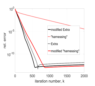
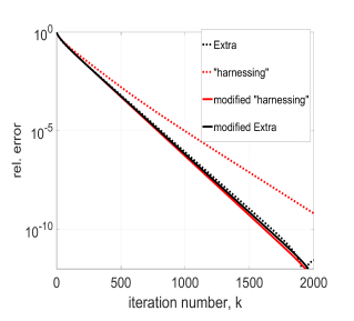
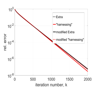
Figure 1: Relative error versus number of iterations $k$, for three different values of step-size $\alpha$: Top: $\alpha=\frac{1}{3\,L}$; middle: $\alpha=\frac{1}{9\,L}$; and bottom: $\alpha=\frac{1}{15\,L}.$

Figure 2 repeats the experiment for a $100$-node, $561$-link, connected network (generated also as an instance of a random geometric graph model with radius $\sqrt{\mathrm{ln}(N)/N}$), and for step-sizes $\alpha=1/(6L)$ (top Figure); $\alpha=1/(18L)$ (middle); and $\alpha=1/(54L)$ (bottom). We can see that a similar behavior of the four methods can be observed here, as well.

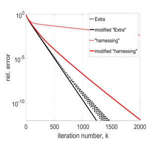
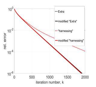
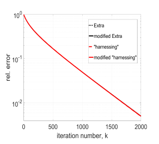
Figure 2: Relative error versus number of iterations $k$, for three different values of step-size $\alpha$: Top: $\alpha=\frac{1}{6\,L}$; middle: $\alpha=\frac{1}{18\,L}$; and bottom: $\alpha=\frac{1}{54\,L}.$

VI Conclusion

We considered exact first order methods for distributed optimization problems where $N$ nodes collaboratively minimize the aggregate sum of their local convex costs. Specifically, we unified, generalized, and improved convergence speed of the existing methods, e.g., [13, 14]. While it was known that the method in [13] is equivalent to a primal-dual gradient-like method, we show here that this is true also with [14], where the corresponding primal-dual update rule incorporates a weighted past dual gradient term, in addition to the current dual gradient term. We then generalize the method by proposing an optimized, easy-to-tune weighting of the past dual gradient term, and show both theoretically and by simulation that the modification yields significant improvements in convergence speed. We establish for the proposed exact method global R-linear convergence rate, assuming strongly convex local costs with Lipschitz continuous gradients and static networks. Possible future work directions include extensions to uncoordinated step-sizes across nodes and time varying, random, and directed networks. Specifically, with directed networks, it would be interesting to extend the methods to work with singly stochastic matrices, i.e., to relax the requirement on the double stochasticity, as doubly stochastic methods become undesirable when dealing with time-varying or directed graph topologies.

.

Appendix

VI-A Proof of Lemma 2

We first prove part (b), i.e., we set $\mathcal{B}=\frac{1}{\alpha}\mathcal{W}$. We must show that (16)–(17) is equivalent to (5)–(II-B). It suffices to show that (16)–(17) is equivalent to (12)–(13), due to Lemma 1. First, note that, due to identity $\mathcal{L}=I-\mathcal{W}$, we have that (16) and (12) are the same. Next, from (16), we have that:

$$\nabla F(x^{(k)})+u^{(k)}=-\frac{1}{\alpha}x^{(k+1)}+\frac{1}{\alpha}\mathcal{W}\,x^{(k)}.$$

Substituting this into (17), and using $\mathcal{B}=\frac{1}{\alpha}\mathcal{W}$, we recover (13). Hence, the equivalence of (16)–(17) and (5)–(II-B) with $\mathcal{B}=\frac{1}{\alpha}\mathcal{W}$. Next, we prove part (a). That is, we consider (14) and (16)–(17) with $\mathcal{B}=0$. The key is to note that $s^{(k)}$, $k=0,1,...,$ can be written as: $s^{(k)}=u^{(k)}+\nabla F(x^{(k)}),$ where $u^{(k)}$ is defined by the following recursion:

$$u^{(k+1)} = \mathcal{W}\,u^{(k)}+(\mathcal{W}-I)\,\nabla F(x^{(k)})$$ (64)

$$= u^{(k)}-\mathcal{L}\,(u^{(k)}+\nabla F(x^{(k)})),$$

for $k=0,1,...,$ and $u^{(0)}=0.$ Substituting (64) into (16), yields the desired equivalence.

VI-B Proof of Lemma 3

Consider (16). Subtracting $x^{\bullet}$ from both sides of the equality, noting that $\mathcal{W}\,x^{\bullet}=x^{\bullet}$, and adding and subtracting $\nabla F(x^{\bullet})$ to the term in the parenthesis on the right hand side of the equality, we obtain:

$$e_{x}^{(k+1)} = \mathcal{W}\,e_{x}^{(k)}-\alpha\,\left(\nabla F(x^{(k)})-\nabla F(x^{\bullet})+\nabla F(x^{\bullet})+u^{(k)}\right)$$ (65)

$$= \mathcal{W}\,e_{x}^{(k)}-\alpha\,\mathcal{H}_{k}\,e_{x}^{(k)}-\alpha\,e_{u}^{(k)},$$

where (65) follows by the definition of $\mathcal{H}_{k}$, $\mathcal{H}_{k}=\int_{t=0}^{1}\nabla^{2}F\left(x^{\bullet}+t\,(x^{(k)}-x^{\bullet})\right)\,dt$, and by the definition of $e_{u}^{(k)}$. Next, consider (17). Using identity $\mathcal{L}=I-\mathcal{W}$, the equality can be equivalently written as:

$$u^{(k+1)}=\mathcal{W}\,u^{(k)}-\mathcal{L}\left(\nabla F(x^{(k)})-\mathcal{B}\,x^{(k)}\right).$$ (66)

Next, add $\nabla F(x^{\bullet})$ to both sides of the equality, and express the quantity on the right hand side as $\nabla F(x^{\bullet})=\mathcal{W}\,\nabla F(x^{\bullet})+\mathcal{L}\,\nabla F(x^{\bullet})$. We obtain:

$$e_{u}^{(k+1)} = \mathcal{W}\,(u^{(k)}+\nabla F(x^{\bullet}))-\mathcal{L}\,\left(\nabla F(x^{(k)})\right.$$ (67)

$$- \left.\nabla F(x^{\bullet})\right)+\mathcal{L}\,\mathcal{B}\,x^{(k)}$$

$$= \mathcal{W}\,e_{u}^{(k)}-\mathcal{L}\,\mathcal{H}_{k}\,e_{x}^{(k)}+\mathcal{L}\,\mathcal{B}\,x^{(k)}.$$

Next, by the property $\mathcal{B}\,x^{\bullet}=c\,x^{\bullet}$, for some $c\in\mathbb{R}$, it follows that: $\mathcal{L}\,\mathcal{B}\,x^{\bullet}$ $=c\,\mathcal{L}\,x^{\bullet}$ $=c\,[\,(I-W)\otimes I\,]\,[\mathbf{1}\otimes x^{\star}]$ $=c\,[\,(I-W)\mathbf{1}\,]\otimes[\,I\otimes x^{\star}\,]=0.$ Hence, we can subtract $\mathcal{L}\,\mathcal{B}\,x^{\bullet}=0$ from the right hand side of (67) to obtain the following:

$$e_{u}^{(k+1)} = \mathcal{W}\,e_{u}^{(k)}-\mathcal{L}\,\mathcal{H}_{k}\,e_{x}^{(k)}+\mathcal{L}\,\mathcal{B}\,e_{x}^{(k)}$$ (68)

$$= \mathcal{W}\,e_{u}^{(k)}+\mathcal{L}\,(\mathcal{B}-\mathcal{H}_{k})\,e_{x}^{(k)}.$$

Finally, note from (68) that:

$$\mathcal{J}\,e_{u}^{(k+1)}=\mathcal{J}\,e_{u}^{(k)},\,\,k=0,1,...,$$

because $\mathcal{J}\,\mathcal{L}=[\,J\otimes I\,]\,[\,(I-W)\otimes I\,]$ $=[\,J(I-W)\,]\otimes I=[J-J]\otimes I=0$. Note that $\mathcal{J}e_{u}^{(0)}=\mathcal{J}(0+\nabla F(x^{\bullet}))=\frac{1}{N}\mathbf{1}(\,\sum_{i=1}^{N}\nabla f_{i}(x^{\star})\,)=0$. Thus, we conclude that $\mathcal{J}\,e_{u}^{(k)}=0$, for all $k$. Applying the latter fact to (68), we obtain:

$$e_{u}^{(k+1)}=(\mathcal{W}-\mathcal{J})\,e_{u}^{(k)}+\mathcal{L}\,(\mathcal{B}-\mathcal{H}_{k})\,e_{x}^{(k)}.$$ (69)

The relations (65) and (69) yield the claim of the Lemma.

VI-C Derivation of the solution to (20) and of an approximate solution to (21)

We first consider (20). Note that, for any $\mathcal{H}\in\mathbb{H}$, we have that: $\|b\,I-\mathcal{H}\|=$ $\max_{i=1,...,Nd}|b-h_{i}|$ $=\max\left\{|b-h_{Nd}|,\,|h_{1}-b|\right\}$ $\leq\max\left\{|b-\mu|,\,|L-b|\right\}.$ Here, $h_{i}$ denotes the $i$-th largest eigenvalue of $\mathcal{H}$. In the last inequality above, we used the fact that $\mu\,I\preceq\mathcal{H}\preceq L\,I$, for all $\mathcal{H}\in\mathbb{H}$. Therefore, we have that:

$$\max_{\mathcal{H}\in\mathbb{H}}\|b\,I-\mathcal{H}\|=\max\{|b-\mu|,\,|L-b|\}.$$ (70)

The maximum in (70) is attained, e.g., for $\mathcal{H}=\mathrm{Diag}(L,\mu,...,\mu)$, where $\mu$ is repeated $(Nd-1)$ times. The quantity (70) is clearly minimized over $b\geq 0$ at $b=b^{\star}=\frac{L+\mu}{2}$.

Now, consider (21), and assume that $\lambda_{N}>0$. Note that the maximal eigenvalue of $\mathcal{W}=W\otimes I$ equals one, and the minimal eigenvalue of $\mathcal{W}$ equals $\lambda_{N}$. We have:

$$\|b^{\prime}\,\mathcal{W}-\mathcal{H}\|\leq\max\left\{|b^{\prime}-\mu|,\,|L-b^{\prime}\,\lambda_{N}|\right\}.$$ (71)

We choose a sub-optimal $b^{\prime}$ that minimizes the upper bound in (71) on the desired function $\sup_{\mathcal{H}\in\mathbb{H}}\|b^{\prime}\,\mathcal{W}-\mathcal{H}\|$. It is easy to see that the corresponding value is $b^{\prime}=\frac{L+\mu}{1+\lambda_{N}}$.

VI-D Proof of equivalence of (16)–(17) and (28)–(III-C)

Consider (16). From the equation, we have: $\nabla F(x^{(k)})+u^{(k)}=-\frac{1}{\alpha}\left(x^{(k+1)}-\mathcal{W}\,x^{(k)}\right).$ Substituting the latter relation in (17), and using the fact that matrices $\mathcal{L}$ and $\mathcal{W}$ commute, as well as that $\mathcal{L}$ and $\mathcal{B}$ commute, (17) leads to (25). Now, consider (28). Proceeding by the same steps as in deriving (12) from (10), it is straightforward to verify that (28) leads to (24). Thus, the equivalence between (16)–(17) and (28)–(III-C). The respective equivalence for the method in [14] follows by setting $\mathcal{B}=0$ in (28)–(29).

VI-E Proof of Theorem 4 for generic matrices $\mathcal{B}$

We show here that, when $\mathcal{B}=b\,I$ is replaced with a generic symmetric matrix $\mathcal{B}$ that respects the sparsity pattern of graph $\mathcal{G}$ and obeys that for any $y\in{\mathbb{R}}^{d}$, there exists some $c\in{\mathbb{R}}$, such that $\mathcal{B}\,(\mathbf{1}\otimes y)=c\,(\mathbf{1}\otimes y)$, Theorem 4 continues to hold with $L^{\prime}$ replaced with constant $\left(L+\|\mathcal{B}\|\right)$. Namely, it is easy to see that Lemma 8 continues to hold unchanged. Further, Lemmas 9–11 pertain to the update equation (16) that does not depend on $\mathcal{B}$, and hence they also hold unchanged. The only modifications occur with Lemma 12. Namely, (61) becomes: $\widetilde{u}^{(k+1)}=$ $\widetilde{\mathcal{W}}\,\widetilde{u}^{(k)}-\mathcal{L}\,(\,\nabla F(x^{(k)})-\nabla F(x^{\bullet})\,)$ $+\mathcal{L}\,\mathcal{B}\,(x^{(k)}-x^{\bullet}).$ Using Lipschitz continuity of $\nabla F$ and the fact that $\|\mathcal{L}\|\leq 2$, the latter equality implies: $\|\widetilde{u}^{(k+1)}\|$ $\leq{\sigma}\,\|\widetilde{u}^{(k)}\|+2\,L\,\|x^{(k)}-x^{\bullet}\|$ $+2\|\mathcal{B}\|\,\|x^{(k)}-x^{\bullet}\|.$ The proof of the modified Lemma 12 then proceeds in the same way as the remaining part of the proof of Lemma 12. Finally, the proof of the modified Theorem 4 then also proceeds in the same way as the proof of Theorem 4.

References

• [1] A. Nedic and A. Ozdaglar, “Distributed subgradient methods for multi-agent optimization,” IEEE Transactions on Automatic Control, vol. 54, no. 1, pp. 48–61, January 2009.
• [2] C. Lopes and A. H. Sayed, “Adaptive estimation algorithms over distributed networks,” in 21st IEICE Signal Processing Symposium, Kyoto, Japan, Nov. 2006.
• [3] F. Cattivelli and A. H. Sayed, “Diffusion LMS strategies for distributed estimation,” IEEE Trans. Sig. Process., vol. 58, no. 3, pp. 1035–1048, March 2010.
• [4] A. H. Sayed, S.-Y. Tu, J. Chen, X. Zhao, and Z. Towfic, “Diffusion strategies for adaptation and learning over networks,” IEEE Sig. Process. Mag., vol. 30, no. 3, pp. 155–171, May 2013.
• [5] J. Duchi, A. Agarwal, and M. Wainwright, “Dual averaging for distributed optimization: Convergence and network scaling,” IEEE Trans. Aut. Contr., vol. 57, no. 3, pp. 592–606, March 2012.
• [6] I. Lobel and A. Ozdaglar, “Convergence analysis of distributed subgradient methods over random networks,” in 46th Annual Allerton Conference onCommunication, Control, and Computing, Monticello, Illinois, September 2008, pp. 353 – 360.
• [7] D. Jakovetic, J. Xavier, and J. M. F. Moura, “Fast distributed gradient methods,” IEEE Trans. Autom. Contr., vol. 59, no. 5, pp. 1131–1146, May 2014.
• [8] ——, “Convergence rates of distributed Nesterov-like gradient methods on random networks,” IEEE Transactions on Signal Processing, vol. 62, no. 4, pp. 868–882, February 2014.
• [9] S. Kar, J. M. F. Moura, and K. Ramanan, “Distributed parameter estimation in sensor networks: Nonlinear observation models and imperfect communication,” IEEE Transactions on Information Theory, vol. 58, no. 6, pp. 3575–3605, June 2012.
• [10] M. Rabbat and R. Nowak, “Distributed optimization in sensor networks,” in IPSN 2004, 3rd International Symposium on Information Processing in Sensor Networks, Berkeley, California, USA, April 2004, pp. 20 – 27.
• [11] S. Boyd, N. Parikh, E. Chu, B. Peleato, and J. Eckstein, “Distributed optimization and statistical learning via the alternating direction method of multipliers,” Foundations and Trends in Machine Learning, Michael Jordan, Editor in Chief, vol. 3, no. 1, pp. 1–122, 2011.
• [12] F. Bullo, J. Cortes, and S. Martinez, Distributed control of robotic networks: A mathematical approach to motion coordination algorithms.   Princeton University Press, 209.
• [13] W. Shi, Q. Ling, G. Wu, and W. Yin, “EXTRA: An exact first-order algorithm for decentralized consensus optimization,” SIAM J. Optim., vol. 25, no. 2, pp. 944 –966, 2015.
• [14] G. Qu and N. Li, “Harnessing smoothness to accelerate distributed optimization,” to appear in IEEE Transactions on Control of Network Systems, 2017, DOI: 10.1109/TCNS.2017.2698261.
• [15] K. Yuan, B. Ying, X. Zhao, and A. H. Sayed, “Exact diffusion for distributed optimization and learning — Part I: Algorithm development,” 2017, arxiv preprint, arXiv:1702.05122.
• [16] ——, “Exact diffusion for distributed optimization and learning — Part II: Convergence analysis,” 2017, arxiv preprint, arXiv:1702.05142.
• [17] D. Jakovetic, J. Xavier, and J. M. F. Moura, “Linear convergence rate of a class of distributed augmented Lagrangian algorithms,” IEEE Trans. Autom. Contr., vol. 60, no. 4, pp. 922–936, April 2015.
• [18] A. Nedic, A. Olshevsky, W. Shi, and C. A. Uribe, “Geometrically convergent distributed optimization with uncoordinated step-sizes,” 2016, arXiv preprint arXiv:1609.05877.
• [19] A. Nedic, A. Olshevsky, and W. Shi, “Achieving geometric convergence for distributed optimization over time-varying graphs,” 2016, arXiv preprint arXiv:1607.03218.
• [20] J. Xu, S. Zhu, Y. Soh, and L. Xie, “Augmented distributed gradient methods for multi-agent optimization under uncoordinated constant stepsizes,” in 54th IEEE Conference on Decision and Control (CDC), 2015, pp. 2055 –2060.
• [21] Q. Lu and H. Li, “Geometrical convergence rate for distributed optimization with time-varying directed graphs and uncoordinated step-sizes,” 2016, arXiv preprint arXiv:1611.00990.
• [22] G. Qu and N. Li, “Accelerated distributed Nesterov gradient descent,” 2017, arxiv preprint arXiv:1705.07176.
• [23] C. Xi and U. A. Khan, “Dextra: A fast algorithm for optimization over directed graphs,” IEEE Transactions on Automatic Control, 2017, to appear, DOI: 10.1109/TAC.2017.2672698.
• [24] J. Zeng and W. Yin, “Extrapush for convex smooth decentralized optimization over directed networks,” Journal of Computational Mathematics, vol. 35, no. 4, pp. 381–394, 2017.
• [25] W. Shi, Q. Ling, G. Wu, and W. Yin, “A proximal gradient algorithm for decentralized composite optimization,” Journal of Machine Learning Research, vol. 63, no. 22, pp. 6013–6023, 2015.
• [26] K. Scaman, F. Bach, S. Bubeck, Y. T. Lee, and L. Massoulie, “Optimal algorithms for smooth and strongly convex distributed optimization in networks,” 2017, arxiv preprint, arXiv:1702.08704.
• [27] A. Nedic, A. Ozdaglar, and A. Parrilo, “Constrained consensus and optimization in multi-agent networks,” IEEE Transactions on Automatic Control, vol. 55, no. 4, pp. 922–938, April 2010.
• [28] A. Mokhtari and A. Ribeiro, “DSA: Decentralized double stochastic averaging gradient algorithm,” Journal of Machine Learning Research, vol. 17, pp. 1–35, 2016.
• [29] A. Nedic and A. Ozdaglar, “Subgradient methods for saddle point problems,” Journal of Optimization Theory and Applications, vol. 145, no. 1, pp. 205– 228, July 2009.
• [30] M. Kallio and C. H. Rosa, “Large-scale convex optimization via saddle-point computation,” Oper. Res., pp. 93– 101, 1999.
• [31] H. Uzawa, “Iterative methods in concave programming,” 1958, in Arrow, K., Hurwicz, L., Uzawa, H. (eds.) Studies in Linear and Nonlinear Programming, pp. 154-165. Stanford University Press, Stanford.
• [32] J. Tsitsiklis, D. Bertsekas, and M. Athans, “Distributed asynchronous deterministic and stochastic gradient optimization algorithms,” IEEE Trans. Autom. Contr., vol. 31, no. 9, pp. 803–812, Sep. 1986.
• [33] Y. E. Nesterov, “A method for solving the convex programming problem with convergence rate O$(1/k^{2})$,” Dokl. Akad. Nauk SSSR, vol. 269, pp. 543 –547, 1983, (in Russian).
• [34] D. Jakovetic, D. Bajovic, N. Krejic, and N. K. Jerinkic, “Distributed gradient methods with variable number of working nodes,” IEEE Transactions on Signal Processing, vol. 64, no. 15, pp. 4080–4095, August 2016.
• [35] M. Zhu and S. Martinez, “On distributed convex optimization under inequality and equality constraints,” IEEE Transactions on Automatic Control, vol. 57, no. 1, pp. 151–164, Jan. 2012.
• [36] T.-H. Chang, A. Nedic, and A. Scaglione, “Distributed constrained optimization by consensus-based primal-dual perturbation method,” IEEE Transactions on Automatic Control, vol. 59, no. 6, pp. 1524–1538, June 2014.
• [37] J. Wang and N. Elia, “Control approach to distributed optimization,” in 48th Annual Allerton Conference onCommunication, Control, and Computing, Monticello, IL, Oct. 2010.
• [38] A. Dimakis, S. Kar, J. M. F. Moura, M. Rabbat, and A. Scaglione, “Gossip algorithms for distributed signal processing,” Proceedings of the IEEE, vol. 98, no. 11, pp. 1847–1864, 2010.
• [39] K. Yuan, Q. Ling, and W. Yin, “On the convergence of decentralized gradient descent,” SIAM J. Optim., vol. 26, no. 3, pp. 1835 –1854, 2016.
• [40] C. Desoer and M. Vidyasagar, Feedback Systems: Input-Output Properties.   SIAM, 2009.
• [41] M. Schmidt, N. L. Roux, and F. Bach, “Convergence rates of inexact proximal-gradient methods for convex optimization,” in Advances in Neural Information Processing Systems 24, 2011, pp. 1458–1466.