Distributed VNF Scaling in Large-scale Datacenters: An ADMM-based Approach

Abstract

Network Functions Virtualization (NFV) is a promising network architecture where network functions are virtualized and decoupled from proprietary hardware. In modern datacenters, user network traffic requires a set of Virtual Network Functions (VNFs) as a service chain to process traffic demands. Traffic fluctuations in Large-scale DataCenters (LDCs) could result in overload and underload phenomena in service chains. In this paper, we propose a distributed approach based on Alternating Direction Method of Multipliers (ADMM) to jointly load balance the traffic and horizontally scale up and down VNFs in LDCs with minimum deployment and forwarding costs. Initially we formulate the targeted optimization problem as a Mixed Integer Linear Programming (MILP) model, which is NP-complete. Secondly, we relax it into two Linear Programming (LP) models to cope with over and underloaded service chains. In the case of small or medium size datacenters, LP models could be run in a central fashion with a low time complexity. However, in LDCs, increasing the number of LP variables results in additional time consumption in the central algorithm. To mitigate this, our study proposes a distributed approach based on ADMM. The effectiveness of the proposed mechanism is validated in different scenarios.

I Introduction

Today, different technologies such as Software Defined Networking (SDN) and Network Function Virtualization (NFV) are being integrated to facilitate the modern datacenter service providers [1]. In these datacenters, the network services are frequently deployed as Virtual Network Function (VNF) chains to process the incoming traffic [2] (see Fig. 1). The NFV architecture relies on off-the-shelf Physical Machines (PMs) which provide computational resources to several Virtual Machines (VMs), each VM implementing a network function with special software programs. In addition, SDN technology could manage the communication network between these VNFs in the datacenter.

Due to traffic fluctuations in datacenters, resource over and underload can occur in service chains. The impact of an overload could be the degradation of overall performance and SLA violations, while underload could lead to significant resource wastage. One of the most popular methods to ensure efficient resource management, is the appropriate placement of VNFs on PMs, which is called the VNF placement problem [3]. This problem has been addressed in literature regarding various parameters, such as network delay and end-to-end latency [4, 5], and operational costs of VNFs (deployment cost, forwarding/processing cost, and energy consumption) [6, 7], and [8]. Although the majority of studies focus on the initial placement of the service chain, network-aware resource management of the service chains during their operational time has emerged as a critical issue. To overcome this issue, the traffic could be load balanced between VNF instances, or the over and underloaded VNF(s) could be scaled up and down. In this paper, we jointly load balance the traffic and horizontally scale up and down VNFs with minimum deployment and forwarding costs. Notably, we use thresholds to automatically detect over and underloaded VM(s), respectively.

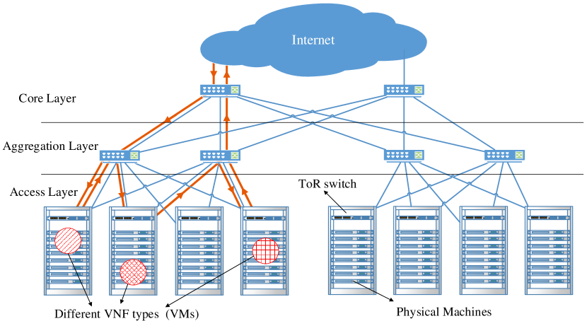
Figure 1: A service chain with three VNFs in a conventional datacenter

Based on the above considerations, the problem is modeled using Mixed Integer Linear Programming (MILP) which is NP-complete [9]. Therefore, we relax our MILP model into two LP formulations. These models perform well in small and medium size datacenters. However, in Large-scale DataCenters (LDCs), the number of variables and constraints of the LP models escalate significantly resulting in an increase in the time complexity of the algorithm, which requires the use of a distributed approach. Hence, we extend our approach to distributed optimization, using a technique known as Alternating Direction Method of Multipliers (ADMM) [10]. In addition to simplicity and its powerfulness, this method has several advantages like fast convergence, low computational complexity, and low overhead of message passing [10]. Using this method, the convex optimization problem is decomposed into different subproblems, each of which is easier to handle. These subproblems are solved iteratively and in parallel using defined agents [10].

Although the conventional ADMM is guaranteed to converge for two-block optimization problems, for n-block variable problems (i.e. multi-block variables) with $n>2$, updating different variables sequentially has no convergence guarantee [11]. Therefore, in this paper, because our problem is in form a of multi-block ADMM, we use a specific ADMM extension called Randomly Permuted ADMM (RP-ADMM) [12] to solve the problem in a distributed way.

Afterall, considering the aforementioned explanations, the main contributions of our proposed work are described as follows:

1. Introducing a joint traffic load balancing and VNF scaling mechanism to mitigate both over and underloaded situations in datacenters,

2. Formulating the above problem as a MILP optimization model, and proposing two LP-relaxations to address time complexity,

3. Extending our approach to a distributed method based on the RP-ADMM technique,

4. Evaluation of the proposed work in different scenarios via simulation.

The remainder of this paper is organized as follows, we start by presenting the related work in the literature (section II). Then, in sections III and IV we illustrate the system model and problem formulation, respectively. Next, the proposed approaches are described in section V. We validate our approach in section VI, and finally, section VII concludes the whole paper.

II Related Work

VM placement has been widely studied in the cloud computing environment [13, 14, 15], and [3]. However, specific characteristics and constraints of the NFV paradigm such as service chaining requirements, deployment and license costs, etc., has made the VNF placement problem more complex. Several studies exist in the literature that tackle this problem. For instance, StEERING [16] focused on VNF chain placement and traffic steering and uses a simple heuristic algorithm to solve the problem. Bari et. al. [6] proposed a model that can be used to determine the optimal number of VNFs and to place them at optimal locations (PMs). In [7], authors modeled this problem to minimize client-server communication distance and operational costs. Also, [17] presented a joint traffic steering and VNF placement using an Integer Linear Programming (ILP) model which sought to minimize the total delay of the traffic. While these approaches largely focus on initial placement of VNFs, they do not monitor VNF chains during their operational time. Hence, because of traffic fluctuations, a resource over or underload could happen in VNF chains, which is a significant challenge to address.

The work most similar to our approach is Stratos [18]. It uses a four-step solution attempting to solve the VNF chain bottlenecks during its operational time. When an overload happens, it initially uses a flow distribution method. When this method fails to solve the bottleneck, Stratos attempts to migrate the VNFs. If the problem persists, Stratos scales up the bottlenecked VNFs. Finally, when all these procedures failed, it scales up all the VNFs in the chain with a fixed number of instances. The primary drawback of Stratos is that it works in a trial manner, which creates resource wastage and inefficiencies to solve the resource bottlenecks. Another close work to us is [19] which attempts to tackle dynamic provisioning of one or multiple service chains in cloud datacenters in a centralized and time-slotted manner. However, [19] does not address the forwarding cost in their model. This could bring additional growth of east-west traffic in the datacenter which increases the wastage of datacenter computation resources [20].

In contrast to afore-mentioned works, we introduce a joint traffic load balancing and VNF scaling mechanism to deal with over and underload phenomena during service chain operational time, while effectively considering forwarding and deployment costs in form of a mathematical optimization model. To the best of our knowledge, there is no literature that is applicable in LDCs. Therefore, we extend the model to a distributed form of optimization, using RP-ADMM method, to be able to use this approach in LDCs.

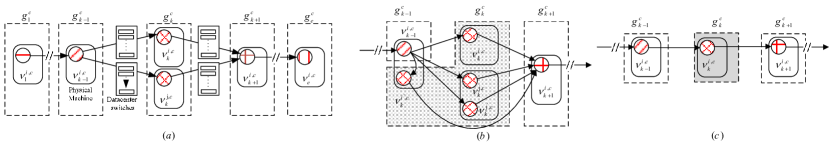
Figure 2: VNF service chain states in a datacenter network, (a) Normal state: an operational VNF chain in a network; (b) Overload occurrence: VMs $i^{\prime}$ and $j^{\prime}$ are launched to manage the overload situation; and (c) Underload occurrence: VM $j$ is turned off to optimize resource usage efficiency in the VNF chain.

III System Model

We consider a datacenter as a graph $\mathscr{G}=\{\mathbb{V},\mathbb{L}\}$, where the vertices set $V$ consists of $U$ physical machines $\mathscr{P}_{i}$ ,$i=1\ldots U$ and $S$ switches $\mathscr{S}_{i}$ ,$i=1\ldots S$, and $\mathbb{L}$ represents edges of $\mathscr{G}$ where $l_{ij}=1$ if a direct communication link exists between two entities $i,j\in\mathbb{V}$. For the ease of problem formulation, we assume a conventional network topology for the datacenter which consists of three layers: access layer, aggregation layer, and core layer (see Fig. 1). The total available resources of a PM is considered as $\mathscr{P}_{i}^{r}$ where $r\in R$ and $R$ is the set of limited types of PM resources such as CPU, memory, bandwidth, etc. Let $C$ be a set of service chains that each of them is constituted by an ordered sequence of VNFs $f_{k}$, where $k\in K$ and $K$ is the set of various network functions such as Firewall, IDS, NAT, etc.

We assume that each VM is providing only one network function. Also, we assume all configured VMs providing network function $k$, are using an identical computational resource. Each VM $i$ that belongs to chain $c\in C$ and provides $f_{k}$, denoted by $v_{k}^{i,c}$, is configured with initial resource $u_{k,r}^{i,c}$ ($r\in R$).

We use the notation $g_{k}^{c}=\{v_{j}^{i,z}\mid\forall j=k,z=c\}$ indicating a set of VMs that provide $f_{k}$ on chain $c\in C$. In addition, ingress and egress points of $g_{k}^{c}$ are defined as $g_{k-1}^{c}$ and $g_{k+1}^{c}$, where $k+1$ and $k-1$ refer to the previous and next service function of $f_{k}$ in chain $c$, respectively. We consider two main phases for each chain: setup phase and operational phase. In setup phase, the requested service chain is deployed in datacenter network with respect to SLA and the available resources of the datacenter. In the second phase, the chain begins to process the incoming traffic, which rate may vary from time to time. Therefore, by having an initial VNF placement for service chains, in this paper, we focus on the second phase of chain lifetime and address the problem of managing the over and underloaded chain with the minimum deployment and forwarding costs.

Our proposed system architecture includes four main components: Monitoring, SDN Controller, VNF Placement and Scaling Module, and REsource Management (REM). Since the proposed approach should respond efficiently and quickly to traffic fluctuations, we use monitoring component to continuously collect the amount of CPU, memory, and bandwidth usage of VMs. In addition to the reported data by monitoring component, the SDN controller collaborates with REM through sharing the routing paths and configuration of network switches. It also updates and configures the routing policy using the REM output. We define $V$ and $V^{*}$ as the set of running VMs in $g_{k}^{c}$ (online VMs), and the set of configured VMs to join $g_{k}^{c}$ (offline VM pool), respectively. Also, let $\tilde{u}_{k,r}^{i,c}$ be the utilization of resource type $r$ of $v_{k}^{i,c}$ in $\tau$ units of time that is measured by monitoring module. Further, we define $\hat{u}_{k,r}^{i,c}$, $\bar{u}_{k,r}^{i,c}$, and $\check{u}_{k,r}^{i,c}$ as hot, warm, and cold thresholds on resource type $r$ for $v_{k}^{i,c}$ to enable us to specify the state of a chain, respectively, as follows:
(1) overload state:

$$\exists k:g_{k}^{c}\in c\mid\exists i:v_{k}^{i,c}\in g_{k}^{c}\text{ and }\tilde{u}_{k,r}^{i,c}\geq\hat{u}_{k,r}^{i,c}$$

(2) underload state:

$$\exists k:g_{k}^{c}\in c\mid\frac{1}{\mid V\mid}\sum_{i:v_{k}^{i,c}\in g_{k}^{c}}\nolimits\tilde{u}_{k,r}^{i,c}\leq\check{u}_{k,r}^{i,c}$$

$$\text{and }max\{\tilde{u}_{k,r}^{i,c}\mid\forall i:v_{k}^{i,c}\in g_{k}^{c}\}\leq\bar{u}_{k,r}^{i,c}$$

(3) normal state: If chain $c$ is neither in overload nor underload state, it is considered being in the normal state.
For illustration, suppose chain $c$ consists of three functions: $f_{1}$, $f_{2}$, and $f_{3}$, where $v_{1}^{1,c}$, $\{v_{2}^{1,c},v_{2}^{2,c}\}$, and $v_{3}^{1,c}$ are serving these functions, respectively. We assume $50\%$, $65\%$ as CPU utilization of $v_{1}^{1,c}$ and $v_{3}^{1,c}$, respectively. In this example, we focus on $f_{2}$ to show how the state of the chain $c$ can be determined. Therefore, we consider the following two scenarios for different CPU utilization of the VMs serving $f_{2}$. Also, we assume hot, warm, and cold thresholds as $90\%$, $80\%$ and $30\%$, respectively. Scenario (a) $\{\tilde{u}_{2,[cpu]}^{1,c}=95\%,\tilde{u}_{2,[cpu]}^{2,c}=75\%\}$: Since the CPU utilization of $v_{2}^{1,c}$ violates the hot threshold, chain $c$ falls into the overload state. We note that the presence of only one violated VM is sufficient to put a chain in the overload state. Scenario (b) $\{\tilde{u}_{2,[cpu]}^{1,c}=40\%,\tilde{u}_{2,[cpu]}^{2,c}=15\%\}$: In this scenario, it can be seen that the average of CPU utilizations is less than the cold threshold. Consequently, this scenario makes chain $c$ to be considered as underload. Notably, $f_{1}$ and $f_{3}$ cannot be in underload state, since there is only one VM assigned for each of these functions.

Remarkably, the values of hot, warm thresholds should be opted in such a way that the gap between their values provides a safety margin to cope with the temporary network traffic fluctuations. Additionally, different types of resources can have different thresholds. For example, the hot thresholds for CPU and memory resources can be set to $90\%$ and $80\%$, respectively [21]. In Fig. 2, we illustrate the three operational states for a sample chain.

IV Problem Formulation

In this section, we address the problem of overload and underload events that occur in network service chain. First, we present a central optimization model, and then extend our study by proposing a distributed model using the ADMM technique. Table I shows the main notations.

To deal with the over/underloaded chain $c$, a number of constraints must be satisfied. Suppose $g_{k}^{c}$ is identified as an over/underloaded set in chain $c$. Let $b_{ij}$ be a binary decision variable, where if $b_{ij}=1$, then VM $j\in\{V\cup V^{*}\}$ must be running on $\mathscr{P}_{i}$. We denote $\alpha_{ij}$ as the percentage of collaboration of VM $j\in\{V\cup V^{*}\}$ on $\mathscr{P}_{i}$, with existing VMs $\in V$ to process the total traffic coming from $g_{k-1}^{c}$. The value of $\alpha_{ij}$ must be restricted as follows:

$$\varepsilon b_{ij}\leq\alpha_{ij}\leq\varphi_{k}b_{ij},\qquad\forall j\in\{V\cup V^{*}\},\forall i\in\mathscr{P}$$ (1)

where $\varepsilon$ shows the minimum amount of collaboration that causes a VM to be launched on a PM. Additionally, $\varphi_{k}$ shows the maximum percentage of service capacity of VMs running network function $k$ in such a way that $\forall j\in\{V\cup V^{*}\}$, $\forall r\in R$, $\varphi_{k}\omega_{k}^{r}T<u_{k,r}^{j,c}$, where $\omega_{k}^{r}$ is defined as the service impact factor of network function $k$ on resource $r\in R$. Let $n_{ij}^{d}$ and $m_{ij}^{d}$, $(i,j\in\{\mathscr{S}\cup\mathscr{P}\}$ and $d\in\{V\cup V^{*}\})$, be the amount of unprocessed traffic rates destined to $v_{k}^{d,c}$, and processed traffic by $v_{k}^{d,c}$ transmitting from $i$ to $j$, respectively. The following constraints state that all online VMs must cover the total traffic flow originated by ingress point $g_{k-1}^{c}$:

$$\sum_{j\in\{V\cup V^{*}\}}\nolimits\sum_{i\in\mathscr{P}}\nolimits\alpha_{ij}=1$$ (2)

$$\sum_{s\in\{\mathscr{S}\cup\mathscr{P}\}}\nolimits l_{si}n_{si}^{j}=T\alpha_{ij},\qquad\forall j\in\{V\cup V^{*}\},\forall i\in\mathscr{P}$$ (3)

where $T$ is the total traffic coming from $g_{k-1}^{c}$ (i.e. ingress point) to the over/underloaded $g_{k}^{c}$. The following constraint indicates that the total required resources for deploying VM(s) on $\mathscr{P}_{i}$ must not be more than its available resources, $\mathscr{P}_{i}^{r}$:

$$\sum_{j\in\{V\cup V^{*}\}}\nolimits b_{ij}u_{k,r}^{j,c}\leq\mathscr{P}_{i}^{r},\hskip 28.45274pt\forall i\in\mathscr{P},r\in R$$ (4)

Additionally, $\forall i\in\mathscr{S}\text{ and }\forall d\in\{V\cup V^{*}\},$ the next constraint is presented as follows:

$$\sum_{j\in\{\mathscr{S}\cup\mathscr{P}\}}\nolimits l_{ij}(n_{ij}^{d}-n_{ji}^{d})=0$$ (5)

$$\sum_{j\in\{\mathscr{S}\cup\mathscr{P}\}}\nolimits l_{ij}(m_{ij}^{d}-m_{ji}^{d})=0$$ (6)

These constraints state that the total incoming (processed and unprocessed) traffic to $\mathscr{S}_{i}$ must be equal to the total outgoing traffic from it. A similar constraint $\forall i\in\mathscr{P}$ and $\forall d\in\{V\cup V^{*}\}$ could be written as follows:

$$\sum_{j\in\{\mathscr{S}\cup\mathscr{P}\}}\nolimits l_{ij}(m_{ij}^{d}-\gamma_{k}n_{ji}^{d})=0$$ (7)

where $\gamma_{k}>0$ is data changing factor of $f_{k}$ serviced by $g_{k}^{c}$ [22]. Although a connection between any pairs of PMs in the datacenter must be established via a switch, the data flow between two different types of VMs, both hosted by an identical PM, is applicable. The following constraints guarantee that the total traffic $T\gamma_{k}$, processed by $g_{k}^{c}$, is received by $g_{k+1}^{c}$ (i.e. egress point):

$$\sum_{d\in\{V\cup V^{*}\}}\nolimits\sum_{i:\mathscr{P}_{i}\in g_{k-1}^{c}}\nolimits\sum_{j\in\{\mathscr{S}\cup\mathscr{P}\}}\nolimits l_{ij}n_{ij}^{d}=T$$ (8)

$$\sum_{d\in\{V\cup V^{*}\}}\nolimits\sum_{i:\mathscr{P}_{i}\in g_{k+1}^{c}}\nolimits\sum_{j\in\{\mathscr{S}\cup\mathscr{P}\}}\nolimits l_{ji}m_{ji}^{d}=T\gamma_{k}$$ (9)

Moreover, $\forall i,j\in\{\mathscr{S}\cup\mathscr{P}\}$ a bandwidth constraint could be formulated as follows:

$$\sum_{d:v_{k}^{d,c}\in g_{k}^{c}}\nolimits l_{ij}(n_{ij}^{d}+m_{ij}^{d})\leq w_{ij}$$ (10)

where $w_{ij}$ is the total available bandwidth of link$(i,j)$. To evaluate the performance of any solutions that satisfies the above constraints, we now propose the following two cost functions:

$$Deployment\text{ }Cost:$$

$$\sum_{i\in\mathscr{P}}\nolimits\sum_{j\in V^{*}}\nolimits b_{ij}\mathbb{X}-\sum_{i\in\mathscr{P}}\nolimits\sum_{j\in V}\nolimits b_{ij}\hat{\mathbb{X}}$$ (11)

$$Forwarding\text{ }Cost:$$

$$\sum_{d\in\{V\cup V^{*}\}}\nolimits\sum_{i\in\{\mathscr{S}\cup\mathscr{P}\}}\nolimits\sum_{j\in\{\mathscr{S}\cup\mathscr{P}\}}\nolimits F(i,j)(n_{ij}^{d}+m_{ij}^{d})$$ (12)

Also, $\mathbb{X}$ and $\hat{\mathbb{X}}$ are considered as two penalty values in the deployment cost formulation. We use the deployment cost to control the power states, migration, and placement of VMs. In fact, it can be utilized for both over and underload situations by adjusting the proper values $\mathbb{X}$ and $\hat{\mathbb{X}}$ (see Proposition. 1 for proof). Further, we use the forwarding cost to force the model to deliver traffic via efficient routes. To achieve this, we should prevent the traffic from being transferred through higher layers of network in the topology (i.e. aggregation and core layers, see Fig. 1). Hence, we defined $F(i,j)$ as the forwarding cost which applies on transmitting composite bit-stream per unit of time, and it is proportional to layers of datacenter topology in which $i$ and $j$ are located. Finally, the following MILP is proposed to jointly balance the traffic load and scale VNFs with the minimum costs:

$$\textit{{minimize}}\qquad\aleph_{1}Eq.(\ref{eq11})+\aleph_{2}Eq.(\ref{eq12})$$ (13)

s.t.

$$Constraints\text{ }(\ref{eq1})-(\ref{eq10})$$

$$\textit{{vars. }}b_{ij}\in\{0,1\},\alpha_{ij},n_{ij}^{d},m_{ij}^{d}\geq 0$$

where $\aleph_{1}$ and $\aleph_{2}$ are two constant weights for deployment and forwarding costs.

Table I: Notations

Notation	Description
$\mathscr{S}_{i}$	The $i^{th}$ switch in datacenter network
$\mathscr{P}_{i}$	The $i^{th}$ physical machine in datacenter network
$R$	The set of resource types (CPU, Memory, etc.)
$K$	The set of network function types
$f_{k}$	The network function type $k\in K$
$l_{ij}$	$l_{ij}=1$ if there is a link between two entities
	$i,j\in\{\mathscr{S}\cup\mathscr{P}\}$
$\mathscr{P}_{i}^{r}$	The total available amount of resource $r\in R$ in $\mathscr{P}_{i}$
$v_{k}^{i,c}$	VM $i$ that belongs to chain $c$ and hosts $f_{k}$
$g_{k}^{c}$	The set of VMs that provide $f_{k}$ on chain $c$
$g_{k-1}^{c}$, $g_{k+1}^{c}$	The ingress/egress points of $g_{k}^{c}$
$\tilde{u}_{k,r}^{i,c}$	The utilization of $r^{th}$ resource of $v_{k}^{i,c}$
$\hat{u}_{k,r}^{i,c}$, $\bar{u}_{k,r}^{i,c}$, $\check{u}_{k,r}^{i,c}$	Hot, warm, and cold thresholds for $r^{th}$ resource of $v_{k}^{i,c}$
$u_{k,r}^{i,c}$	The initial resource type $r$ for $v_{k}^{i,c}$
$n_{ij}^{d}$	The amount of unprocessed traffic destined to $v_{k}^{d,c}$
	transmitting from $i$ to $j$, where $i,j\in\{\mathscr{S}\cup\mathscr{P}\}$
$m_{ij}^{d}$	The amount of processed traffic by $v_{k}^{d,c}$ transmitting
	from $i$ to $j$ where $i,j\in\{\mathscr{S}\cup\mathscr{P}\}$
$T$	The total traffic received by $g_{k}^{c}$
$\gamma_{k}$	Traffic changing factor of $f_{k}$
$\alpha_{ij}$	The percentage of collaboration of $v_{k}^{j,c}$, hosted on
	$\mathscr{P}_{i}$, with other VMs providing identical network
	function and belong to $g_{k}^{c}$
$\varphi_{k}$	The maximum percentage of service capacity of
	VMs running network function $k$
$\omega_{k}^{r}$	The service impact factor of network function $k$ on
	resource $r\in R$
$b_{ij}$	$b_{ij}=1$ if VM $j$ is hosted by $\mathscr{P}_{i}$
$w_{ij}$	Total available bandwidth of link$(i,j)$, $i,j\in\{\mathscr{S}\cup\mathscr{P}\}$
$v^{*}$	The number of required VNFs to process the received
	traffic by $g_{k}^{c}$
$V$, $V^{*}$	Online VMs belongs to $g_{k}^{c}$, offline VM pool for $g_{k}^{c}$
$\Psi$, $\Psi^{*}$	The set of PMs hosting $V$ and candidate PMs for
	hosting $V^{*}$
$e_{ij}$	The amount of interest of each PM $\in\{\Psi\cup\Psi^{*}\}$ in
	processing the incoming traffic

Proposition 1. The proposed MILP model (13) could be used to mitigate both over and underloaded service chains with adjusting the appropriate penalty values of $\mathbb{X}$ and $\hat{\mathbb{X}}$.

Proof:

Suppose $g_{k}^{c}$ is an over/underloaded set which serves VNF type $k$ in chain $c$. In Eq. (11), we presented the deployment cost that consists of two terms: the first term handles the online VMs, $v_{k}^{i,c}\in g_{k}^{c}$, and the second term focuses on offline VM instances of $k$ which are ready to be transferred to a PM and start servicing in $g_{k}^{c}$. In the presence of an overload, there is a solution that jointly balances the traffic rates among the online VMs, and launches one or more offline VMs. Considering overall cost, by choosing two positive values for $\mathbb{X}$ and $\hat{\mathbb{X}}$, where $\hat{\mathbb{X}}\gg\mathbb{X}$, the MILP overcomes overload using flow distribution on online VMs, horizontal scaling, and migration, respectively. On the other hand, when an underload is detected, the best solution is to turn off one or more online VMs and load balance the traffic rates among the remained online VMs. To preserve the resource efficiency, there is no need to turn on new VM instances, unless migrating a VM dramatically decreases the forwarding cost. Hence, the value of $\hat{\mathbb{X}}$ must be set to a large negative number while $\mathbb{X}$ should remain as a very large positive number. ∎

Considering the aforementioned observations, by detecting over/underloaded chain, the REM adjusts the proper values for $\mathbb{X}$ and $\hat{\mathbb{X}}$ and triggers the optimization algorithm.

V The Proposed Approach

Since the proposed MILP model (13) is NP-complete and suffers from high time complexity [9], we consider two linear relaxations of the MILP model to address over and underloaded VNFs. These LP models could be centrally run in small or even medium size datacenters. However, using these models in LDCs is not applicable due to increasing the number of variables and constraints. Thus, we extend our study by proposing a distributed mechanism based on the RP-ADMM technique.

V-A The Central Design

In case of an overloaded $g_{k}^{c}$, suppose that the number of required VNFs $f_{k}$, which is denoted by $v^{*}$, to process the received traffic equals to $Max\{\lceil T\omega_{k}^{r}/u_{k,r}^{j,c}\rceil\mid\forall r\in R\}$. Also, we define $\Psi$ and $\Psi^{*}$ sets, which are the set of PMs that are hosting $V$, and the set of candidate PMs that has adequate resources to host at least one VM $\in V^{*}$, respectively. The relaxed overload model of MILP (13) is presented as follows:

The overload LP model:

$$\textit{{minimize}}\qquad Eq.(\ref{eq12})$$ (14)

s.t.

$$Constraints\hskip 5.2pt(\ref{eq5})-(\ref{eq9})\hskip 125.0pt\text{(I)-(V)}$$

$$\alpha_{ij}-\alpha_{qj}=0,\hskip 21.90874pti=|V|+1:v^{*},\forall j,q\in\{\Psi\cup\Psi^{*}\}\hskip 5.69046pt(\text{VI})$$

$$\sum_{q\in\{\Psi\cup\Psi^{*}\}}\nolimits e_{qj}-\alpha_{ij}=0,\ \hskip 1.42271pti=1:v^{*},\forall j\in\{\Psi\cup\Psi^{*}\}\text{(VII)}$$

$$\sum_{s\in\{\mathscr{S}\cup\mathscr{P}\}}\nolimits l_{si}n_{si}^{j}-Te_{ij}=0,$$

$$\hskip 91.04872pti=|V|+1:v^{*},\forall j\in\{\Psi\cup\Psi^{*}\}\hskip 2.84544pt(\text{VIII})$$

$$\sum_{s\in\{\mathscr{S}\cup\mathscr{P}\}}\nolimits l_{si}n_{si}^{j}-T\alpha_{ij}=0,\hskip 17.64056pti=1:|V|,\forall j\in\Psi\hskip 7.11317pt(\text{IX})$$

$$\textit{{vars. }}\hskip 28.45274ptn_{ij}^{d},m_{ij}^{d}\geq 0,0\leq\alpha_{ij}\leq\varphi_{k},0\leq e_{ij}\leq 1$$

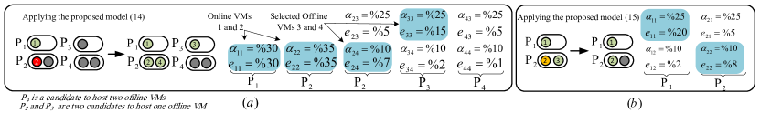
Figure 3: An example of over and underloaded chains and their solution, (a) The overload case (b) The underload case

Since the number of desired VMs is known, the deployment cost in the objective function could be omitted. In fact, having $v^{*}$, the relaxed overload model (14) specifically focuses on the forwarding cost. In this model, the routing constraints could be used as they were before, except the bandwidth constraint (Eq. (10)). We ignored the bandwidth constraint in the proposed relaxed models. However, we will relax this assumption in our future work. Additionally, to relax the binary variable $b_{ij}$ in the MILP model (13), we define $e_{ij}\in\mathbb{R}^{+}$ as a new variable in which $j=1:v^{*}$, and $i\in\{\Psi\cup\Psi^{*}\}$. This variable identifies the amount of interest of each PM in processing the incoming traffic. For each required instance $j$, the PM with the highest value of $e_{ij}$ is selected to run the $j^{th}$ VM instance and handle $T\alpha_{ij}$ of traffic (constraints (VI)-(VIII)). Finally, constraint (IX) determines the amount of received traffic that must be processed by each PM $i\in\Psi$.

On the other hand, when an underload occurs, the following LP-relaxation model, which can be obtained easily from the above model, runs on the first $v^{*}$ online VMs to appropriately assign them to PMs $\in\Psi$ and distribute received load from $g_{k-1}^{c}$ on $g_{k}^{c}$:

The underload LP model:

$$\textit{{minimize}}\qquad Eq.(\ref{eq12})$$ (15)

s.t.

$$Constraints\text{ }(\ref{eq5})-(\ref{eq9})\hskip 127.0pt\text{(I)-(V)}$$

$$\alpha_{ij}-\alpha_{qj}=0,\hskip 72.55461ptj=1:v^{*},\forall i,q\in\Psi\hskip 14.22636pt\text{(VI)}$$

$$\sum_{q\in\Psi}\nolimits e_{qj}-\alpha_{ij}=0,\hskip 50.3615ptj=1:v^{*},\forall i\in\Psi\hskip 11.38092pt\text{(VII)}$$

$$\sum_{s\in\{\mathscr{S}\cup\mathscr{P}\}}\nolimits l_{si}n_{si}^{j}-Te_{ij}=0,\hskip 17.07182pti=1:v^{*},\forall j\in\Psi\hskip 8.5359pt\text{(VIII)}$$

$$\textit{{vars. }}\hskip 19.91684ptn_{ij}^{d},m_{ij}^{d}\geq 0,0\leq\alpha_{ij}\leq\varphi_{k},0\leq e_{ij}\leq 1$$

For clarification on details of the proposed models, an example for overloaded and underloaded chains is shown in Fig. 3. In Fig. 3(a), the overloaded $g_{k}^{c}$ has two VMs $(1,2)\in V$, which are running on $(\mathscr{P}_{1},\mathscr{P}_{2})\in\Psi$, respectively. By assuming overloaded VM 2 and setting $v^{*}=4$, two extra VMs $(3,4)\in V^{*}$ with the same VNF type must be added to $g_{k}^{c}$ regarding $(\mathscr{P}_{2},\mathscr{P}_{3},\mathscr{P}_{4})\in\Psi^{*}$. Obtained $\alpha_{ij}$ and $e_{ij}$, VMs 3 and 4 are selected to be launched on $\mathscr{P}_{3}$ and $\mathscr{P}_{2}$, respectively. Additionally, in Fig. 3(b), a final decision has been made based on the calculated values of $e_{ij}$ and $\alpha_{ij}$ for the underloaded chain. In this case, the relaxed underload LP model turns off VM 3 running on $\mathscr{P}_{2}$.

V-B Introducing ADMM

After many years without too much attention, the ADMM technique has recently witnessed a renaissance in many application areas [11]. Generally, there are two types of distributed methods: Sub-gradient and ADMM. The best known rate of convergence for sub-gradient methods is $O(\frac{1}{\sqrt{\ell}})$, while the ADMM algorithm converges at the rate $O(\frac{1}{\ell})$ for the general case, where $\ell$ is the number of iterations [23]. Therefore, since both approaches are iteration-based and the speed of convergence in the ADMM is more than the sub-gradient method, we develop our distributed approach based on the ADMM algorithm.

We first introduce the background of the ADMM and then apply it to design our distributed algorithm. Consider the following convex minimization problem with a separable objective function and linear constraints:

minimize $$f_{1}(x_{1})+f_{2}(x_{2})+...+f_{n}(x_{n}),$$ (16)

s.t. $$A_{1}x_{1}+A_{2}x_{2}+...+A_{n}X_{n}=b,$$

vars. $$x_{i}\in\mathscr{X}_{i},i=1,...,n,$$

where $A_{i}\in\mathbb{R}^{N\times d_{i}}$, $b\in\mathbb{R}^{N\times 1}$, $\mathscr{X}_{i}\subseteq\mathbb{R}^{d_{i}}$ is a closed convex set, and $f_{i}:\mathbb{R}^{d_{i}}\rightarrow\mathbb{R}$ is a closed convex function, $i=1,...,n$ [12]. In case of $n=2$ (i.e. two blocks of variables), the augmented Lagrangian function for model (16) can be written as follows:

$$L_{\beta}(x_{1},x_{2},\mu)= f_{1}(x_{1})+f_{2}(x_{2})+\mu^{\intercal}(A_{1}x_{1}+A_{2}x_{2}-b)$$

$$+\frac{\beta}{2}\parallel A_{1}x_{1}+A_{2}x_{2}-b\parallel_{2}^{2}$$ (17)

where $\mu$ is the Lagrangian multiplier and $\beta$ is the positive penalty scalar. The two-block ADMM updates the primal variables $x_{1}$ and $x_{2}$, followed by a dual variable update $\mu$ in an iterative manner. By having $(x_{1}^{0},x_{2}^{0},\mu^{0})$ as an initial vector, the updated variables at iteration $\ell>0$ are computed in an alternating fashion as follows:

$$x_{1}^{\ell}= \operatorname*{argmin}\limits_{x_{1}}L_{\beta}(x_{1},x_{2}^{\ell-1},\mu^{\ell-1})$$ (18)

$$x_{2}^{\ell}= \operatorname*{argmin}\limits_{x_{2}}L_{\beta}(x_{1}^{\ell},x_{2},\mu^{\ell-1})$$ (19)

$$\mu^{\ell}= \mu^{\ell-1}-\beta(A_{1}x_{1}^{\ell}+A_{2}x_{2}^{\ell}-b)$$ (20)

Separable structure of convex model (16) allows ADMM to decompose it over its primal variables and achieve the optimal solution in a distributed way. To formulate the ADMM into a scaled form that is more convenient to be used in designing algorithm, we define $u=(\frac{1}{\beta})\mu$ as the scaled dual variable. Thus, we have:

$$\mu^{\intercal}(A_{1} x_{1}+A_{2}x_{2}-b)+\frac{\beta}{2}\parallel A_{1}x_{1}+A_{2}x_{2}-b\parallel_{2}^{2}$$

$$=\frac{\beta}{2}\parallel A_{1}x_{1}+A_{2}x_{2}-b+u\parallel_{2}^{2}-\frac{\beta}{2}\parallel u\parallel_{2}^{2}$$ (21)

By disregarding independent terms of the minimization variables, the ADMM method could be expressed as:

$$x_{1}^{\ell}=\operatorname*{argmin}\limits_{x_{1}}(f_{1}(x_{1}) +(\frac{\beta}{2})\parallel A_{1}x_{1}+A_{2}x_{2}^{\ell-1}$$

$$-b+u^{\ell-1}\parallel_{2}^{2})$$ (22)

$$x_{2}^{\ell}=\operatorname*{argmin}\limits_{x_{2}}(f_{2}(x_{2}) +(\frac{\beta}{2})\parallel A_{1}x_{1}^{\ell}+A_{2}x_{2}$$

$$-b+u^{\ell-1}\parallel_{2}^{2})$$ (23)

$$u^{\ell}=u^{\ell-1}+A_{1}x_{1}^{\ell}+A_{2}x_{2}^{\ell}-b$$ (24)

The optimality and convergence of the two-block ADMM for model (16) is proved in [10] under mild technical assumptions.

On the other hand, many applications need more than two blocks of variables to be considered (i.e. $n>2$). By direct extending of ADMM to multi-block case, the convergence cannot be established well [11]. The authors in [12] proposed Randomly Permuted ADMM (RP-ADMM), as a simple modification in updating process of primal variables to make the convergence possible in a desirable duration. In fact, RP-ADMM draw a permutation $\Omega$ of $\{1,...,n\}$ uniformly at random and update the primal variables in the order of the permutation, followed by updating the dual variables in a usual way [12]. Since our proposed approach has more than two blocks of variables, we apply RP-ADMM technique to solve the problem in a distributed way.

V-C Applying RP-ADMM

In this section, we develop our distributed algorithm based on the proposed model (14). We firstly reformulate the proposed model (14) to an applicable model for applying RP-ADMM, and then introduce our RP-ADMM-based distributed algorithm.

Since $\forall j\in\{\mathscr{S}\cup\Psi\cup\Psi^{*}\}$, each node $i\in\{\mathscr{S}\cup\Psi\cup\Psi^{*}\}$ is responsible to determine its local flow variables $n_{ij}^{d}$ and $m_{ij}^{d}$ in a distributed manner, we have to reformulate flow conservation constraints (I)-(V) in (14). So, by introducing auxiliary variables $A_{ij}^{d}$, $B_{ij}^{d}$, and $C_{ij}^{d}$, we reform constraints (I)-(III), $j\in\{\mathscr{S}\cup\Psi\cup\Psi^{*}\},d=1:v^{*}$, where $l_{ij}=1$, as follows:

$$n_{ij}^{d}-n_{ji}^{d}-A_{ij}^{d}=0,\hskip 27.03003pt\forall i\in\mathscr{S}$$ (25)

$$\sum_{j\in\{\mathscr{S}\cup\Psi\cup\Psi^{*}\}}\nolimits A_{ij}^{d}=0$$ (26)

$$m_{ij}^{d}-m_{ji}^{d}-B_{ij}^{d}=0,\hskip 21.33955pt\forall i\in\mathscr{S}$$ (27)

$$\sum_{j\in\{\mathscr{S}\cup\Psi\cup\Psi^{*}\}}\nolimits B_{ij}^{d}=0$$ (28)

$$m_{ij}^{d}-\gamma_{k}n_{ji}^{d}-C_{ij}^{d}=0,\hskip 14.79555pt\forall i\in\mathscr{P}$$ (29)

$$\sum_{j\in\{\mathscr{S}\cup\Psi\cup\Psi^{*}\}}\nolimits C_{ij}^{d}=0$$ (30)

Without loss of generality, assume that ingress and egress points of $g_{k}^{c}$ have one PM indexed by 0 and 1, respectively. To reform constraints (IV) and (V) in (14), we similarly define two more auxiliary variables $D_{d}$ and $E_{d}$, $(d=1:v^{*})$:

$$\sum_{j\in\{\mathscr{S}\cup\mathscr{P}_{0}\}}\nolimits l_{0j}n_{0j}^{d}-D_{d}=0$$ (31)

$$\sum_{d=1:v^{*}}\nolimits D_{d}-T=0$$ (32)

$$\sum_{j\in\{\mathscr{S}\cup\mathscr{P}_{1}\}}\nolimits l_{j1}m_{j1}^{d}-E_{d}=0$$ (33)

$$\sum_{d=1:v^{*}}\nolimits E_{d}-T\gamma_{k}=0$$ (34)

Now, the RP-ADMM can be easily applied on the following model:

minimize $$Eq.(\ref{eq12})$$ (35)

s.t. $$Eq.(\ref{eq25})\text{ - }Eq.(\ref{eq340}),$$

constraints (VI) - (IX) in model (14)

vars. $$n_{ij}^{d},m_{ij}^{d},A_{ij}^{d},B_{ij}^{d},C_{ij}^{d},D_{d},E_{d}\geq 0,$$

$$0\leq\alpha_{ij}\leq\varphi_{k},0\leq e_{ij}\leq 1$$

The augmented Lagrangian function for the model (35) can be presented as follows:

$$L_{\beta}(n,m,A,B,C,D,E,\alpha,e;$$ (36)

$$\delta,\bar{\delta},\eta,\bar{\eta},\zeta,\bar{\zeta},\lambda_{0},\bar{\lambda}_{0},\lambda_{1},\bar{\lambda}_{1},\mu,\xi,\sigma,\rho)=Eq.(\ref{eq12})$$

$$+\delta^{\intercal}Eq.(\ref{eq25})+\frac{\beta}{2}\parallel Eq.(\ref{eq25})\parallel_{2}^{2}+\bar{\delta}^{\intercal}Eq.(\ref{eq260})+\frac{\beta}{2}\parallel Eq.(\ref{eq260})\parallel_{2}^{2}$$

$$+\eta^{\intercal}Eq.(\ref{eq26})+\frac{\beta}{2}\parallel Eq.(\ref{eq26})\parallel_{2}^{2}+\bar{\eta}^{\intercal}Eq.(\ref{eq270})+\frac{\beta}{2}\parallel Eq.(\ref{eq270})\parallel_{2}^{2}$$

$$+\zeta^{\intercal}Eq.(\ref{eq27})+\frac{\beta}{2}\parallel Eq.(\ref{eq27})\parallel_{2}^{2}+\bar{\zeta}^{\intercal}Eq.(\ref{eq300})+\frac{\beta}{2}\parallel Eq.(\ref{eq300})\parallel_{2}^{2}$$

$$+\lambda_{0}^{\intercal}Eq.(\ref{eq28})+\frac{\beta}{2}\parallel Eq.(\ref{eq28})\parallel_{2}^{2}+\bar{\lambda}_{0}^{\intercal}Eq.(\ref{eq280})+\frac{\beta}{2}\parallel Eq.(\ref{eq280})\parallel_{2}^{2}$$

$$+\lambda_{1}^{\intercal}Eq.(\ref{eq29})+\frac{\beta}{2}\parallel Eq.(\ref{eq29})\parallel_{2}^{2}+\bar{\lambda}_{1}^{\intercal}Eq.(\ref{eq340})+\frac{\beta}{2}\parallel Eq.(\ref{eq340})\parallel_{2}^{2}$$

$$+\mu^{\intercal}\text{Cons. (VI, model (\ref{eq14}))}+\frac{\beta}{2}\parallel\text{Cons. (VI model (\ref{eq14}))}\parallel_{2}^{2}$$

$$+\xi^{\intercal}\text{Cons. (VII, model (\ref{eq14}))}+\frac{\beta}{2}\parallel\text{Cons. (VII model (\ref{eq14}))}\parallel_{2}^{2}$$

$$+\sigma^{\intercal}\text{Cons. (VIII, model (\ref{eq14}))}+\frac{\beta}{2}\parallel\text{Cons. (VIII model (\ref{eq14}))}\parallel_{2}^{2}$$

$$+\rho^{\intercal}\text{Cons. (IX, model (\ref{eq14}))}+\frac{\beta}{2}\parallel\text{Cons. (IX model (\ref{eq14}))}\parallel_{2}^{2}$$

where $\delta,\bar{\delta},\eta,\bar{\eta},\zeta,\bar{\zeta},\lambda_{0},\bar{\lambda}_{0},\lambda_{1},\bar{\lambda}_{1},\mu,\xi,\sigma$, and $\rho$ are the Lagrangian multiplier and $\beta$ is the positivie penalty scalar.

Considering the above explanations, we are able to utilize the n-block RP-ADMM algorithm to distributedly solve the model (35) (see Algorithm 1). As illustrated in Algorithm 1, it starts by initializing primal and dual variables in the first line. In line 2, we defined an array to store the last values of the variables (primal and dual). The iterative process begins in line 3 where $\ell$ indicates the round number. In each round, RP-ADMM algorithm picks a uniformly random permutation $\Omega$ to specify the order of updating primal variables. In fact, the inner $for$ loop (lines 6 to 10), selects the $\Omega(i)^{th}$ variable to update its value in $\ell^{th}$ round by considering the last value of variables stored in the LastValueArray. Then, in line 9 the value of $\Omega(i)^{th}$ primal variable is overwrited. For illustration, suppose that $\Omega=\{3,4,2,1\}$ ($n=4$) and $\ell=12$. Therefore, according to the order of $\Omega$, the third primal variable (i.e. $\Omega(1)^{th}$ variable) must be updated first, followed by fourth, second, and first primal variable. Also, in this round, for example, the second variable updating process uses the current values (computed in 12^th round) of third and forth variables, and also the obtained value of the first variable in previous round (i.e. 11^th round). Using the scaled form of ADMM algorithm, the primal variables are updated as follows:

Updating Switches Primal Variables: If the selected variable belongs to the set of network switches, each switch $i$, updates its traffic flow rate variable to its neighbor $j\in\{\mathscr{S}\cup\Psi\cup\Psi^{*}\}$ using the following equations:

$$n_{ij}^{d(\ell)}=\operatorname*{argmin}\limits_{n_{ij}^{d}}(Eq.(\ref{eqlag}))$$

$$\hskip 19.91684pt=\operatorname*{argmin}\limits_{n_{ij}^{d}}(Eq.(\ref{eq12})+\frac{\beta}{2}\parallel n_{ij}^{d}-n_{ji}^{d(\ell^{*})}-A_{ij}^{d(\ell^{*})}$$

$$+\frac{1}{\beta}\delta_{ij}^{d(\ell^{*})}\parallel_{2}^{2}+\frac{\beta}{2}\parallel n_{ji}^{d(\ell^{*})}-n_{ij}^{d}-A_{ji}^{d(\ell^{*})}+\frac{1}{\beta}\delta_{ji}^{d(\ell^{*})}\parallel_{2}^{2}$$

$$+\frac{\beta}{2}\parallel m_{ji}^{d(\ell^{*})}-\gamma_{k}n_{ij}^{d}-C_{ji}^{d(\ell^{*})}+\frac{1}{\beta}\zeta_{ji}^{d(\ell^{*})}\parallel_{2}^{2}+\frac{\beta}{2}\parallel n_{ij}^{d}$$

$$+\sum_{s\in\{\mathscr{S}\cup\Psi\cup\Psi^{*}\},s\neq i}\nolimits l_{sj}n_{sj}^{d(\ell^{*})}-Te_{jd}^{\ell^{*}}+\frac{1}{\beta}\sigma_{j}^{d(\ell^{*})}\parallel_{2}^{2}$$

$$+\operatorname*{\Theta}\limits_{j\in\Psi}\frac{\beta}{2}\parallel n_{ij}^{d}+\sum_{s\in\{\mathscr{S}\cup\Psi\cup\Psi^{*}\},s\neq i}\nolimits l_{sj}n_{sj}^{d(\ell^{*})}-T\alpha_{jd}^{(\ell^{*})}$$

$$+\frac{1}{\beta}\rho_{j}^{d(\ell^{*})}\parallel_{2}^{2})$$ (37)

where $\operatorname*{\Theta}\limits_{X}$ plays as an if statement; i.e. it returns 1 if condition ”X” is true. Also, $a^{d(\ell^{*})}$ or $a^{(\ell^{*})}$ shows the most recent value of the primal variable $a$, stored in LastValueArray. Similarly, $m_{ij}^{d(\ell)}$, $A_{ij}^{d(\ell)}$, and $B_{ij}^{d(\ell)}$ are obtained from the following equations:

$$m_{ij}^{d(\ell)}=\operatorname*{argmin}\limits_{m_{ij}^{d}}(Eq.(\ref{eq12})+\frac{\beta}{2}\parallel m_{ij}^{d}-m_{ji}^{d(\ell^{*})}-B_{ij}^{d(\ell^{*})}$$

$$+\frac{1}{\beta}\eta_{ij}^{d(\ell^{*})}\parallel_{2}^{2}+\frac{\beta}{2}\parallel m_{ji}^{d(\ell^{*})}-m_{ij}^{d}-B_{ij}^{d(\ell^{*})}+\frac{1}{\beta}\eta_{ji}^{d(\ell^{*})}\parallel_{2}^{2}$$

$$+\operatorname*{\Theta}\limits_{j=1}\frac{\beta}{2}\parallel m_{ij}^{d}+\sum_{s\in\{\mathscr{S}\cup\mathscr{P}_{1}\},s\neq i}\nolimits l_{sj}m_{sj}^{d(\ell^{*})}-E_{d}^{(\ell^{*})}$$

$$+\frac{1}{\beta}\lambda_{j}^{d(\ell^{*})}\parallel_{2}^{2})$$ (38)

$$A_{ij}^{d(\ell)}=\operatorname*{argmin}\limits_{A_{ij}^{d}}(\frac{\beta}{2}\parallel n_{ij}^{d(\ell^{*})}-n_{ji}^{d(\ell^{*})}-A_{ij}^{d}+\frac{1}{\beta}\delta_{ij}^{d(\ell^{*})}\parallel_{2}^{2}$$

$$+\frac{\beta}{2}\parallel A_{ij}^{d}+\sum_{s\in\{\mathscr{S}\cup\Psi\cup\Psi^{*}\},s\neq j}\nolimits A_{is}^{d(\ell^{*})}+\frac{1}{\beta}\bar{\delta}_{i}^{d(\ell^{*})}\parallel_{2}^{2})$$ (39)

$$B_{ij}^{d(\ell)}=\operatorname*{argmin}\limits_{B_{ij}^{d}}(\frac{\beta}{2}\parallel m_{ij}^{d(\ell^{*})}-m_{ji}^{d(\ell^{*})}-B_{ij}^{d}+\frac{1}{\beta}\eta_{ij}^{d(\ell^{*})}\parallel_{2}^{2}$$

$$+\frac{\beta}{2}\parallel B_{ij}^{d}+\sum_{s\in\{\mathscr{S}\cup\Psi\cup\Psi^{*}\},s\neq j}\nolimits B_{is}^{d(\ell^{*})}+\frac{1}{\beta}\bar{\eta}_{i}^{d(\ell^{*})}\parallel_{2}^{2})$$ (40)

1 Initialize: $n_{ij}^{d(0)}$, $m_{ij}^{d(0)}$, $\alpha_{ij}^{d(0)}$, $e_{ij}^{d(0)}$, $A_{ij}^{d(0)}$, $B_{ij}^{d(0)}$, $C_{ij}^{d(0)}$, $D_{d}^{(0)}$, $E_{d}^{(0)}$ and dual variables

2 LastValueArray[] = initialized variables;

3 for $\ell=1,2,...$ do

4       $n$=length(primal variables);

5       Pick a permutation $\Omega$ of $\{1,...,n\}$ uniformly at random;

6       for $i=1:n$ do

7             //Updating primal variables:

8             Update the $\Omega(i)^{th}$ primal variable;

9             Update LastValueArray[$\Omega(i)$];

10            

11       end for

12      Update dual variables;

13      

14 end for

Algorithm 1 n-block RP-ADMM

Updating PMs Primal Variables: If the selected variable belongs to the set of PMs, each PM $i$ updates the primal dual variables $n_{ij}^{d}$, $m_{ij}^{d}$, $\alpha_{id}$, $e_{id}$, $C_{ij}^{d(\ell)}$, $D_{d}^{(\ell)}$, and $E_{d}^{\ell}$ using the following equations:

$$n_{ij}^{d(\ell)}=\operatorname*{argmin}\limits_{n_{ij}^{d}}(Eq.(\ref{eq12})+\frac{\beta}{2}\parallel n_{ji}^{d(\ell^{*})}-n_{ij}^{d}-A_{ji}^{d(\ell^{*})}$$

$$+\frac{1}{\beta}\delta_{ji}^{d(\ell^{*})}\parallel_{2}^{2}+\operatorname*{\Theta}\limits_{i=0}\frac{\beta}{2}\parallel n_{ij}^{d}+\sum_{s\in\{\mathscr{S}\cup\mathscr{P}_{0}\},s\neq j}\nolimits l_{is}n_{is}^{d(\ell^{*})}$$

$$-D_{d}^{(\ell^{*})}+\frac{1}{\beta}\lambda_{0}^{d(\ell^{*})}\parallel_{2}^{2}+\frac{\beta}{2}\parallel n_{ij}^{d}$$

$$+\sum_{s\in\{\mathscr{S}\cup\Psi\cup\Psi^{*}\},s\neq i}\nolimits l_{sj}n_{sj}^{d(\ell^{*})}-Te_{jd}^{d(\ell^{*})}+\frac{1}{\beta}\sigma_{j}^{d(\ell^{*})}\parallel_{2}^{2}$$

$$+\frac{\beta}{2}\parallel n_{ij}^{d}+\sum_{s\in\{\mathscr{S}\cup\Psi\cup\Psi^{*}\},s\neq i}\nolimits l_{sj}n_{sj}^{d(\ell^{*})}-T\alpha_{jd}^{d(\ell^{*})}$$

$$+\frac{1}{\beta}\rho_{j}^{d(\ell^{*})}\parallel_{2}^{2})$$ (41)

$$m_{ij}^{d(\ell)}=\operatorname*{argmin}\limits_{m_{ij}^{d}}(Eq.(\ref{eq12})+\frac{\beta}{2}\parallel m_{ji}^{d(\ell^{*})}-m_{ij}^{d}-B_{ji}^{d(\ell^{*})}$$

$$+\frac{1}{\beta}\eta_{ji}^{d(\ell^{*})}\parallel_{2}^{2}+\frac{\beta}{2}\parallel m_{ij}^{d}-\gamma_{k}n_{ij}^{d(\ell^{*})}-C_{ij}^{d(\ell^{*})}+\frac{1}{\beta}\zeta_{ij}^{d(\ell^{*})}\parallel_{2}^{2}$$

$$+\operatorname*{\Theta}\limits_{i=1}\frac{\beta}{2}\parallel m_{ij}^{d}+\sum_{s\in\{\mathscr{S}\cup\mathscr{P}_{1}\},s\neq i}\nolimits l_{sj}m_{sj}^{d(\ell^{*})}-E_{d}^{(\ell^{*})}$$

$$+\frac{1}{\beta}\lambda_{i}^{d(\ell^{*})}\parallel_{2}^{2})$$ (42)

$$\alpha_{id}^{(\ell)}=\operatorname*{argmin}\limits_{\alpha_{id}}(\operatorname*{\Theta}\limits_{d>|V|}\frac{\beta}{2}\sum_{q\in\{\Psi\cup\Psi^{*}\},q\neq i}\nolimits\parallel\alpha_{id}-\alpha_{qd}^{(\ell^{*})}$$

$$+\frac{1}{\beta}\mu_{iq}^{d(\ell^{*})}\parallel_{2}^{2}+\frac{\beta}{2}\parallel\sum_{q\in\{\Psi\cup\Psi^{*}\}}\nolimits e_{qd}^{(\ell^{*})}-\alpha_{id}+\frac{1}{\beta}\xi_{i}^{d(\ell^{*})}\parallel_{2}^{2}$$

$$+\operatorname*{\Theta}\limits_{i\in\Psi}\frac{\beta}{2}\parallel\sum_{s\in\{\mathscr{S}\cup\Psi\cup\Psi^{*}\}}\nolimits l_{si}n_{si}^{d(\ell^{*})}-T\alpha_{id}+\frac{1}{\beta}\rho_{i}^{d(\ell^{*})}\parallel_{2}^{2})$$ (43)

$$e_{id}^{(\ell)}=\operatorname*{argmin}\limits_{e_{id}}(\frac{\beta}{2}\parallel e_{id}+\sum_{q\in\{\Psi\cup\Psi^{*}\},q\neq i}\nolimits e_{id}^{(\ell^{*})}-\alpha_{qd}^{(\ell^{*})}$$

$$+\frac{1}{\beta}\xi_{i}^{d(\ell^{*})}\parallel_{2}^{2}+\operatorname*{\Theta}\limits_{d>|V}\frac{\beta}{2}\parallel\sum_{s\in\{\mathscr{S}\cup\Psi\cup\Psi^{*}\}}\nolimits l_{si}n_{si}^{d(\ell^{*})}-Te_{id}$$

$$+\frac{1}{\beta}\sigma_{i}^{d(\ell^{*})}\parallel_{2}^{2})$$ (44)

$$C_{ij}^{d(\ell)}=\operatorname*{argmin}\limits_{C_{ij}^{d}}(\frac{\beta}{2}\parallel m_{ij}^{d(\ell^{*})}-\gamma_{k}n_{ji}^{d(\ell^{*})}-C_{ij}^{d}+\frac{1}{\beta}\zeta_{ij}^{d(\ell^{*})}\parallel_{2}^{2}$$

$$+\frac{\beta}{2}\parallel C_{ij}^{d}+\sum_{s\in\{\mathscr{S}\cup\Psi\cup\Psi^{*}\},s\neq j}\nolimits C_{is}^{d(\ell^{*})}+\frac{1}{\beta}\bar{\zeta}_{i}^{d(\ell^{*})}\parallel_{2}^{2})$$ (45)

In case of $i\in ingress$, we should update $D_{d}^{(\ell)}$ as below:

$$D_{d}^{(\ell)}=\operatorname*{argmin}\limits_{D_{d}}(\frac{\beta}{2}(\parallel\sum_{s\in\{\mathscr{S}\cup\mathscr{P}_{0}\}}\nolimits l_{is}n_{is}^{d(\ell^{*})}-D_{d}$$

$$+\frac{1}{\beta}\lambda_{i}^{d(\ell^{*})}\parallel_{2}^{2}+\parallel D_{d}+\sum_{s=1:v^{*},s\neq d}\nolimits D_{s}^{(\ell^{*})}-T$$

$$+\frac{1}{\beta}\bar{\lambda}_{i}^{(\ell^{*})}\parallel_{2}^{2}))$$ (46)

However, if $i\in egress$, $E_{d}^{(\ell)}$ should be updated as follows:

$$E_{d}^{(\ell)}=\operatorname*{argmin}\limits_{E_{d}}(\frac{\beta}{2}(\parallel\sum_{s\in\{\mathscr{S}\cup\mathscr{P}_{1}\}}\nolimits l_{si}m_{si}^{d(\ell^{*})}-E_{d}$$

$$+\frac{1}{\beta}\lambda_{i}^{d(\ell^{*})}\parallel_{2}^{2}+\parallel E_{d}+\sum_{s=1:v^{*},s\neq d}\nolimits E_{s}^{(\ell^{*})}-T$$

$$+\frac{1}{\beta}\bar{\lambda}_{i}^{(\ell^{*})}\parallel_{2}^{2}))$$ (47)

Finally, in line 11 of Algorithm 1, the dual variables can be updated as follows:

• $\forall i\in\mathscr{S}$ and $\forall j\in\{\mathscr{S}\cup\Psi\cup\Psi^{*}\}:$

$$\delta_{ij}^{d(\ell)}=\delta_{ij}^{d(\ell-1)}+\beta(n_{ij}^{d(\ell)}-n_{ji}^{d(\ell)}-A_{ij}^{d(\ell)})$$ (48)

$$\bar{\delta_{i}}^{d(\ell)}=\bar{\delta_{i}}^{d(\ell-1)}+\beta(\sum_{s\in\{\mathscr{S}\cup\mathscr{P}\}}\nolimits A_{is}^{d(\ell)})$$ (49)

$$\eta_{ij}^{d(\ell)}=\eta_{ij}^{d(\ell-1)}+\beta(m_{ij}^{d(\ell)}-m_{ji}^{d(\ell)}-B_{ij}^{d(\ell)})$$ (50)

$$\bar{\eta_{i}}^{d(\ell)}=\bar{\eta_{i}}^{d(\ell-1)}+\beta(\sum_{s\in\{\mathscr{S}\cup\mathscr{P}\}}\nolimits B_{is}^{d(\ell)})$$ (51)

• $\forall i\in\{\Psi\cup\Psi^{*}\}\text{ and }\forall j\in\{\mathscr{S}\cup\Psi\cup\Psi^{*}\}:$

$$\zeta_{ij}^{d(\ell)}=\zeta_{ij}^{d(\ell-1)}+\beta(m_{ij}^{d(\ell)}-\gamma_{k}n_{ji}^{d(\ell)}-C_{ij}^{d(\ell)})$$ (52)

$$\bar{\zeta_{i}}^{d(\ell)}=\bar{\zeta_{i}}^{d(\ell-1)}+\beta(\sum_{s\in\{\mathscr{S}\cup\mathscr{P}\}}\nolimits C_{il}^{d(\ell)})$$ (53)

$$\sigma_{i}^{d(\ell)}=\sigma_{i}^{d(\ell-1)}+\beta(\sum_{s\in\{\mathscr{S}\cup\mathscr{P}\}}\nolimits l_{si}n_{si}^{d(\ell)}-Te_{id}^{(\ell)})$$ (54)

$$\mu_{ij}^{d(\ell)}=\mu_{ij}^{d(\ell-1)}+\beta(\alpha_{id}^{(\ell)}-\alpha_{jd}^{(\ell)})$$ (55)

$$\xi_{i}^{d(\ell)}=\xi_{i}^{d(\ell-1)}+\beta(\sum_{l\in\{\Psi\cup\Psi^{*}\}}\nolimits e_{ld}^{d(\ell)}-\alpha_{id}^{(\ell)})$$ (56)

• If $(i\in ingress):$

$$\lambda_{0}^{d(\ell)}=\lambda_{0}^{d(\ell-1)}+\beta(\sum_{s\in\{\mathscr{S}\cup\mathscr{P}_{0}\}}\nolimits l_{0s}n_{0s}^{d(\ell)}-D_{d}^{(\ell)})$$ (57)

$$\bar{\lambda}_{0}^{(\ell)}=\bar{\lambda}_{0}^{(\ell-1)}+\beta(\sum_{d=1:v^{*}}\nolimits D_{d}^{(\ell)})$$ (58)

• If $(i\in egress):$

$$\lambda_{1}^{d(\ell)}=\lambda_{1}^{d(\ell-1)}+\beta(\sum_{s\in\{\mathscr{S}\cup\mathscr{P}_{1}\}}\nolimits l_{s1}m_{s1}^{d(\ell)}-E_{d}^{(\ell)})$$ (59)

$$\bar{\lambda}_{1}^{(\ell)}=\bar{\lambda_{1}}^{(\ell-1)}+\beta(\sum_{d=1:v^{*}}\nolimits E_{d}^{(\ell)})$$ (60)

• If $(i\in\Psi):$

$$\rho_{i}^{d(\ell)}=\rho_{i}^{d(\ell-1)}+\beta(\sum_{s\in\{\mathscr{S}\cup\mathscr{P}\}}\nolimits l_{si}n_{si}^{d(\ell)}-T\alpha_{id}^{(\ell)})$$ (61)

Table II: Comparing time complexities of proposed models in different topologies

				MILP (13)		LP (Overload) (14)		LP (Underload) (15)
$k$-fat-tree	No. of Switches	No. of PMs	No. of Variables	No. of Constraints	Run time (s)	No. of Constraints	Run time (s)	No. of Constraints	Run Time (s)
2	5	4	120	25	0.555	68	0.075	62	0.055
4	20	16	672	315	5.064	254	0.614	188	0.318
8	80	64	4224	1251	323.523	998	14.977	692	6.635
16	320	256	29184	4995	$N/A$	3974	974.235	2708	456.674
32	1280	1024	129024	19971	$N/A$	15878	$N/A$	10772	$N/A$
64	5120	4096	466944	79875	$N/A$	63494	$N/A$	43028	$N/A$

Clearly, the primal values of the RP-ADMM model can be updated according to the selected permutation. In case of overload, when $v_{k}^{i,c}$ violates the defined threshold, it determines $v^{*}$ and then triggers PMs $\in\{\Psi\cup\Psi^{*}\}$ and some adjacent switches via sending a simple packet. Then, the RP-ADMM update process can be launched considering the selected PMs and switches.

VI Performance Evaluation

To assess the performance of the proposed approach, we simulate the proposed MILP, LP, and ADMM models utilizing MATLAB software. We conducted our simulation on a hardware composing of an INTEL Core i7 1.73GHz CPU, 8GB of RAM, and Windows 10 x64 OS. We considered $k$-fat-tree topologies as the datacenter network structure. In general, a $k-fat-tree$ has $k/2$ ToR and aggregate switches in each pod, and $k^{2}/4$ core switches [24]. We mainly use 4-ary fat-tree topology for performance evaluation (see Fig. 4). However, we run some of our experiments based on different topology sizes (i.e. 8, 16, 32, and 64-ary fat-trees). Also $\tau$ is considered as 5 seconds for all runs.

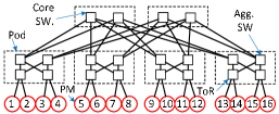
Figure 4: 4-fat-tree topology

In our first experiment, we investigate the performances of MILP (13), LP (14), and (15) models in terms of the number of variables, constraints, and execution time on various k-fat-trees. We consider $g_{c}^{k}$ with two VMs (i.e. $|V|=2$), $|\Psi|=2$, $|V^{*}|=1$, and each rack equipped with two PMs. As it can be seen in Table II, number of switches, PMs, variables, and constraints are proportional to the size of datacenter (i.e. $k$-fat-tree). Obviously, for larger datacenters, the execution time of the proposed models also increased specifically for MILP model. Table II clearly implies that in LDCs, we need to apply an efficient distributed algorithm to achieve a solution in a reasonable time.

As another experiment, we consider a 4-fat-tree topology to evaluate the performance of the proposed LP models for over and underloaded chains in different scenarios. Each of these scenarios is designed based on the number of PMs in $g_{k}^{c}$, ingress and egress points, $\Psi^{*}$ (i.e. the candidate PMs that are able to launch new VMs), normalized ($0\sim 1$) forwarding costs (N. FwdCost), and $v^{*}$ (the number of required VNFs to process the received traffic by $g_{k}^{c}$) for overload and underload cases (see column 1-4 in Table III). We also considered the forwarding costs between different layers of datacenter as: PM-ToR=10, ToR-Aggregation=20, and Aggregation-Core=40. Further, to simulate overload and underload cases, we increased the traffic rate by $50\%$ (for each extra VM) and decreased it by $50\%$, respectively.

The normalized forwarding cost and its increase/decrease rates are shown in Table III. We also configured the initial parameters in such a way that LP is forced to turn on/off VMs to mitigate the over or underload $g_{k}^{c}$. Overall, Table III shows how LP models react to over/underloaded chains by turning on/off offline/online VMs. In case of overload, the proposed LP model (14) prefers to launch a VM on ingress and egress PMs in order to minimize the traffic forwarding cost. In fact, the traffic between two different VNFs on an identical PM (i.e. ingress or egress) is negligible due to an internal traffic handling. For instance, in the first scenario in Table III ($\mathscr{P}_{1}\rightarrow(\mathscr{P}_{2},\mathscr{P}_{5})\rightarrow\mathscr{P}_{4}$), when we need to turn on two more VMs for $g_{k}^{c}$ (i.e. $v^{*}=4$), the LP model (14) selects $\mathscr{P}_{1}$ and $\mathscr{P}_{4}$ (i.e. ingress and egress points, respectively) to launch the new VMs ($\mathscr{P}_{1}\rightarrow(\boldsymbol{\mathscr{P}_{1}},\mathscr{P}_{2},\mathscr{P}_{5},\boldsymbol{\mathscr{P}_{4}})\rightarrow\mathscr{P}_{4}$). Also, it can be seen that by using this new configuration, the forwarding cost increases by $20\%$, which is caused by the increased amount of network traffic. In addition, it can be seen that in the third scenario ($\mathscr{P}_{1}\rightarrow(\mathscr{P}_{1},\mathscr{P}_{2})\rightarrow\mathscr{P}_{2}$), the maximum increase in forwarding cost is resulted among all scenarios ($116\%$). This is because, the utilized PMs before chain overload (i.e. $\mathscr{P}_{1}$ and $\mathscr{P}_{2}$) were on a same rack, while after running LP model (14), two more PMs (i.e. $\mathscr{P}_{3}$ and $\mathscr{P}_{4}$) are use to handle the traffic, which are stored on another rack. It is noticeable that we assumed that only $\mathscr{P}_{3}-\mathscr{P}_{16}$ PMs can afford enough resources to launch new VMs (i.e. $\Psi^{*}=\{\mathscr{P}_{3}-\mathscr{P}_{16}\}$). On the other hand, when an underload occurs, the LP model (15) prefers to turn off a VM that has the most forwarding cost. For example, in the first scenario, $\mathscr{P}_{5}$ is turned off. Because $\mathscr{P}_{5}$ is in pod 2, so the traffic should pass the higher layers of network (i.e. aggregate and core layers) to reach the next hop in the chain (i.e. $\mathscr{P}_{4}$). Also, as it can be seen in the last column of Table III, the forwarding cost decreases by $14\%$. Additionally, it can be seen that maximum forwarding cost reduction took place in the last scenario. The reason is that the LP model (15) turns off the VMs on $\mathscr{P}_{3}$ and $\mathscr{P}_{4}$, which are stored in another rack. Therefore, the traffic is not passing the higher network layers and as a result, the forwarding cost in the chain reduces significantly.

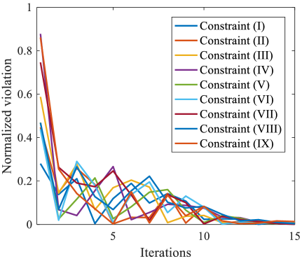
Figure 5: The normalized violation of the constraints in model (14)

One of the well-known features of ADMM is its fast convergence which is clearly illustrated in Fig. 6. For declaration, we focused on the last scenario in Table (III) and compared the optimal cost value obtained by LP model (14) with the solution of distributed ADMM algorithm (we set $\beta=5$). According to Fig. 6, the distributed ADMM converges to the optimal value in 15 iterations. This low number of iterations indicates that the proposed distributed ADMM technique can perform well with low overhead (e.g. message passing) in a LDC. Notably, we set the stop criterion to 25 iterations. In addition, in Fig. 5 we measure the normalized violation of each constraint in model (14) to show how fast violations decrease.

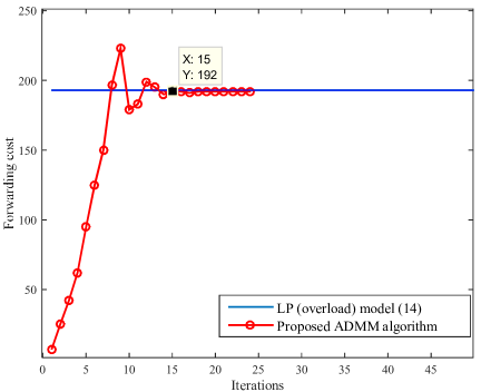
Figure 6: The convergence rate of the proposed distributed RP-ADMM algorithm

Table III: Comparing the results of LP models in different scenarios

$g_{k-1}^{c}\rightarrow(g_{k}^{c})\rightarrow g_{k+1}^{c}$	N. FwdCost	LP overload model (14)				LP underload model (15)
		$\Psi^{*}$	$v^{*}$	New Configuration	FwdCost	$v^{*}$	New Configuration	FwdCost
$\mathscr{P}_{1}\rightarrow(\mathscr{P}_{2},\mathscr{P}_{5})\rightarrow\mathscr{P}_{4}$	0.68	ALL PMs	3	$\mathscr{P}_{1}\rightarrow(\mathscr{P}_{2},\mathscr{P}_{5},\boldsymbol{\mathscr{P}_{4}})\rightarrow\mathscr{P}_{4}$	+14%	1	$\mathscr{P}_{1}\rightarrow(\mathscr{P}_{2})\rightarrow\mathscr{P}_{4}$	-14%
			4	$\mathscr{P}_{1}\rightarrow(\boldsymbol{\mathscr{P}_{1}},\mathscr{P}_{2},\mathscr{P}_{5},\boldsymbol{\mathscr{P}_{4}})\rightarrow\mathscr{P}_{4}$	+20%
$\mathscr{P}_{1}\rightarrow(\mathscr{P}_{1},\mathscr{P}_{2},\mathscr{P}_{3})\rightarrow\mathscr{P}_{16}$	1	$\mathscr{P}_{3}-\mathscr{P}_{16}$	4	$\mathscr{P}_{1}\rightarrow(\mathscr{P}_{1},\mathscr{P}_{2},\mathscr{P}_{3},\boldsymbol{\mathscr{P}_{16}})\rightarrow\mathscr{P}_{16}$	+11%	2	$\mathscr{P}_{1}\rightarrow(\mathscr{P}_{1},\mathscr{P}_{2})\rightarrow\mathscr{P}_{4}$	-6%
			5	$\mathscr{P}_{1}\rightarrow(\mathscr{P}_{1},\mathscr{P}_{2},\mathscr{P}_{3},\boldsymbol{\mathscr{P}_{3}},\boldsymbol{\mathscr{P}_{16}})\rightarrow\mathscr{P}_{16}$	+17%	1	$\mathscr{P}_{1}\rightarrow(\mathscr{P}_{1})\rightarrow\mathscr{P}_{4}$	-16%
$\mathscr{P}_{1}\rightarrow(\mathscr{P}_{1},\mathscr{P}_{2})\rightarrow\mathscr{P}_{2}$	0.23	ALL PMs	3	$\mathscr{P}_{1}\rightarrow(\mathscr{P}_{1},\boldsymbol{\mathscr{P}_{1}},\mathscr{P}_{2})\rightarrow\mathscr{P}_{2}$	+25%	1	$\mathscr{P}_{1}\rightarrow(\mathscr{P}_{1})\rightarrow\mathscr{P}_{2}$	-33%
		$\mathscr{P}_{3}-\mathscr{P}_{16}$	4	$\mathscr{P}_{1}\rightarrow(\mathscr{P}_{1},\mathscr{P}_{1},\boldsymbol{\mathscr{P}_{3}},\boldsymbol{\mathscr{P}_{4}})\rightarrow\mathscr{P}_{2}$	+116%
$\mathscr{P}_{1}\rightarrow(\mathscr{P}_{3},\mathscr{P}_{5},\mathscr{P}_{6})\rightarrow\mathscr{P}_{2}$	0.77	$\mathscr{P}_{2}-\mathscr{P}_{16}$	4	$\mathscr{P}_{1}\rightarrow(\boldsymbol{\mathscr{P}_{2}},\mathscr{P}_{3},\mathscr{P}_{5},\mathscr{P}_{6})\rightarrow\mathscr{P}_{2}$	+13%	2	$\mathscr{P}_{1}\rightarrow(\mathscr{P}_{3},\mathscr{P}_{5})\rightarrow\mathscr{P}_{2}$	-9%
		$\mathscr{P}_{3}-\mathscr{P}_{16}$	5	$\mathscr{P}_{1}\rightarrow(\mathscr{P}_{3},\boldsymbol{\mathscr{P}_{3}},\boldsymbol{\mathscr{P}_{4}},\mathscr{P}_{5},\mathscr{P}_{6})\rightarrow\mathscr{P}_{2}$	+30%	1	$\mathscr{P}_{1}\rightarrow(\mathscr{P}_{3})\rightarrow\mathscr{P}_{2}$	-36%

VII Conclusion

Today, the integration of NFV and SDN introduces a new distinguished, yet challenging networking architecture. One of these challenges is VNF over and underloads in the network during their operational time. This problem could increase resource wastage, SLA violations, and also decrease efficiency. In this paper, we conducted a theoretical study of the VNF scaling problem with the aim of minimizing deployment and forwarding costs in a datacenter. In fact, we addressed the aforementioned issue by presenting a jointly traffic load balancing and VNF scaling mechanism to overcome both over and underload phenomena in datacenters. In this regard, we formulated the problem as a MILP optimization model. Also, to cope with the time complexity of MILP, we relaxed it into two LP models. However, in LDCs, there are huge number of network switches and servers, that increase the number of constraints and variables in LP models significantly. Hence, the proposed central LP model is practically useless for LDCs. Therefore, we extend our approach to a distributed method based on the ADMM technique. However, the conventional ADMM is guaranteed to converge for two-block variables problem, while for multi-block variable problems, updating different variables sequentially has no convergence guarantee. Hence, because our problem is formulated in a multi-block variable form, we used an extension of the ADMM technique, called Randomly Permuted ADMM (RP-ADMM) to solve the problem in a distributed manner. To the best of our knowledge, our work is the first one to tackle this problem using a distributed optimization approach. We evaluated the performance of the presented models numerically in different scenarios based on k-fat-tree topology. The results validated the performance of our proposed algorithms. The most important part of our future work is to implement the introduced distributed approach in real-world test beds. On the other hand, considering a workload prediction module in our architecture is worth to be explored in future. In this way, we would be able to predict the traffic load and adjust VNF placement in advance. Additionally, the performance (e.g., end-to-end delay) is also a critical factor in forwarding path selection of service chains. In fact, it would influence the selection of candidate PMs and VMs. Therefore, it could be considered as an extension to the mathematical formulation as another future direction.

VIII Acknowledgement

We are grateful to Islamic Azad University, Mashhad branch authorities, for their useful collaboration. This work has been partly supported by the German Federal Ministry of Education and Research (BMBF) under the project SEcure Networking for a DATa center cloud in Europe (SENDATE) (Project ID 16KIS0261).

References

• [1] Rashid Mijumbi, Joan Serrat, Juan-Luis Gorricho, Niels Bouten, Filip De Turck, and Raouf Boutaba. Network function virtualization: State-of-the-art and research challenges. IEEE Communications Surveys & Tutorials, 18(1):236–262, 2015.
• [2] Dilip A Joseph, Arsalan Tavakoli, and Ion Stoica. A policy-aware switching layer for data centers. In ACM SIGCOMM Computer Communication Review, volume 38, pages 51–62. ACM, 2008.
• [3] Arsany Basta, Wolfgang Kellerer, Marco Hoffmann, Hans Jochen Morper, and Klaus Hoffmann. Applying nfv and sdn to lte mobile core gateways, the functions placement problem. In Proceedings of the 4th workshop on All things cellular: operations, applications, & challenges, pages 33–38. ACM, 2014.
• [4] Dilip Krishnaswamy, Ravi Kothari, and Vijay Gabale. Latency and policy aware hierarchical partitioning for nfv systems. In Network Function Virtualization and Software Defined Network (NFV-SDN), 2015 IEEE Conference on, pages 205–211. IEEE, 2015.
• [5] Minh-Tuan Thai, Ying-Dar Lin, and Yuan-Cheng Lai. A joint network and server load balancing algorithm for chaining virtualized network functions. In 2016 IEEE International Conference on Communications (ICC), pages 1–6. IEEE, 2016.
• [6] Md Bari, Shihabur Rahman Chowdhury, Reaz Ahmed, Raouf Boutaba, et al. On orchestrating virtual network functions in nfv. IEEE Transactions on Network and Service Management, 2015.
• [7] Rami Cohen, Liane Lewin-Eytan, Joseph Seffi Naor, and Danny Raz. Near optimal placement of virtual network functions. In 2015 IEEE Conference on Computer Communications (INFOCOM), pages 1346–1354. IEEE, 2015.
• [8] Milad Ghaznavi, Aimal Khan, Nashid Shahriar, Khalid Alsubhi, Reaz Ahmed, and Raouf Boutaba. Elastic virtual network function placement. In Cloud Networking (CloudNet), 2015 IEEE 4th International Conference on, pages 255–260. IEEE, 2015.
• [9] Stephen A Vavasis. Nonlinear optimization: complexity issues. Oxford University Press, Inc., 1991.
• [10] Stephen Boyd, Neal Parikh, Eric Chu, Borja Peleato, and Jonathan Eckstein. Distributed optimization and statistical learning via the alternating direction method of multipliers. Foundations and Trends in Machine Learning, 3(1):1–122, 2011.
• [11] Caihua Chen, Bingsheng He, Yinyu Ye, and Xiaoming Yuan. The direct extension of admm for multi-block convex minimization problems is not necessarily convergent. Mathematical Programming, 155(1-2):57–79, 2016.
• [12] Ruoyu Sun, Zhi-Quan Luo, and Yinyu Ye. On the expected convergence of randomly permuted admm. arXiv preprint arXiv:1503.06387, 2015.
• [13] Joe Wenjie Jiang, Tian Lan, Sangtae Ha, Minghua Chen, and Mung Chiang. Joint vm placement and routing for data center traffic engineering. In INFOCOM, 2012 Proceedings IEEE, pages 2876–2880. IEEE, 2012.
• [14] Xiaoqiao Meng, Vasileios Pappas, and Li Zhang. Improving the scalability of data center networks with traffic-aware virtual machine placement. In INFOCOM, 2010 Proceedings IEEE, pages 1–9. IEEE, 2010.
• [15] Amir Varasteh and Maziar Goudarzi. Server consolidation techniques in virtualized data centers: A survey. IEEE Systems Journal, 2015.
• [16] Ying Zhang, Neda Beheshti, Ludovic Beliveau, Geoffrey Lefebvre, Ravi Manghirmalani, Ramesh Mishra, Ritun Patneyt, Meral Shirazipour, Ramesh Subrahmaniam, Catherine Truchan, et al. Steering: A software-defined networking for inline service chaining. In 2013 21st IEEE International Conference on Network Protocols (ICNP), pages 1–10. IEEE, 2013.
• [17] Marcelo Caggiani Luizelli, Leonardo Richter Bays, Luciana Salete Buriol, Marinho Pilla Barcellos, and Luciano Paschoal Gaspary. Piecing together the nfv provisioning puzzle: Efficient placement and chaining of virtual network functions. In 2015 IFIP/IEEE International Symposium on Integrated Network Management (IM), pages 98–106. IEEE, 2015.
• [18] Aaron Gember, Anand Krishnamurthy, Saul St John, Robert Grandl, Xiaoyang Gao, Ashok Anand, Theophilus Benson, Aditya Akella, and Vyas Sekar. Stratos: A network-aware orchestration layer for middleboxes in the cloud. Technical report, Technical Report, 2013.
• [19] Xiaoke Wang, Chuan Wu, Franck Le, Alex Liu, Zongpeng Li, and Francis Lau. Online vnf scaling in datacenters. arXiv preprint arXiv:1604.01136, 2016.
• [20] Po-Wen Chi, Yu-Cheng Huang, and Chin-Laung Lei. Efficient nfv deployment in data center networks. In 2015 IEEE International Conference on Communications (ICC), pages 5290–5295. IEEE, 2015.
• [21] Zhen Xiao, Weijia Song, and Qi Chen. Dynamic resource allocation using virtual machines for cloud computing environment. IEEE Transactions on parallel and distributed systems, 24(6):1107–1117, 2013.
• [22] Wenrui Ma, Carlos Medina, and Deng Pan. Traffic-aware placement of nfv middleboxes. In 2015 IEEE Global Communications Conference (GLOBECOM), pages 1–6. IEEE, 2015.
• [23] Ermin Wei and Asuman Ozdaglar. Distributed alternating direction method of multipliers. In 2012 IEEE 51st IEEE Conference on Decision and Control (CDC), pages 5445–5450. IEEE, 2012.
• [24] Praveen Tammana, Rachit Agarwal, and Myungjin Lee. Cherrypick: Tracing packet trajectory in software-defined datacenter networks. In Proceedings of the 1st ACM SIGCOMM Symposium on Software Defined Networking Research, page 23. ACM, 2015.