Distributed second order methods with increasing number of working nodes

Abstract

Recently, an idling mechanism has been introduced in the context of distributed first order methods for minimization of a sum of nodes’ local convex costs over a generic, connected network. With the idling mechanism, each node $i$, at each iteration $k$, is active – updates its solution estimate and exchanges messages with its network neighborhood – with probability $p_{k}$, and it stays idle with probability $1-p_{k}$, while the activations are independent both across nodes and across iterations. In this paper, we demonstrate that the idling mechanism can be successfully incorporated in distributed second order methods also. Specifically, we apply the idling mechanism to the recently proposed Distributed Quasi Newton method (DQN). We first show theoretically that, when $p_{k}$ grows to one across iterations in a controlled manner, DQN with idling exhibits very similar theoretical convergence and convergence rates properties as the standard DQN method, thus achieving the same order of convergence rate (R-linear) as the standard DQN, but with significantly cheaper updates. Simulation examples confirm the benefits of incorporating the idling mechanism, demonstrate the method’s flexibility with respect to the choice of the $p_{k}$’s, and compare the proposed idling method with related algorithms from the literature.

I Introduction

Context and motivation. The problem of distributed minimization of a sum of nodes’ local costs across a (connected) network has received a significant and growing interest in the past decade, e.g., [1, 2, 3, 4]. Such problem arises in various application domains, including wireless sensor networks, e.g., [5], smart grid, e.g., [6], distributed control applications, e.g., [7], etc.

In the recent paper [8], a class of novel distributed first order methods has been proposed, motivated by the so-termed “hybrid” methods in [9] for (centralized) minimization of a sum $\sum_{i=1}^{n}f_{i}(x)$ of convex component functions. The main idea underlying a hybrid method in [9] is that it is designed as a combination of 1) an incremental or stochastic gradient method (or, more generally, an incremental or stochastic Newton-like method) and 2) a full (standard) gradient method (or a standard Newton-like method); it behaves as the stochastic method at the initial algorithm stage, and as the standard method at a later stage. An advantage of the hybrid method is that it potentially inherits some favorable properties of both incremental/stochastic and standard methods, while eliminating their important drawbacks. For example, the hybrid exhibits fast convergence at initial iterations $k$ while having inexpensive updates, just like incremental/stochastic methods. On the other hand, it eliminates the oscillatory behavior of incremental methods around the solution for large $k$’s (because for large $k$’s it behaves as a full/standard method). Hybrid methods calculate a search direction at iteration $k$ based on a subset (sample) of the $f_{i}$’s, where the sample size is small at the initial iterations (mimicking a stochastic/incremental method), while it approaches the full sample $n$ for large $k$’s (essentially matching a full, standard method).

With distributed first order methods in [8], the sample size at iteration $k$ translates into the number of nodes that participate in the distributed algorithm at $k$. More precisely, therein we introduce an idling mechanism where each node in the network at iteration $k$ is active with probability $p_{k}$ and stays idle with probability $1-p_{k}$, where $p_{k}$ is nominally increasing to one with $k$, while the activations are independent both across nodes and through iterations. Reference [8] analyzes convergence rates for a distributed gradient method with the idling mechanism and demonstrates by simulation that idling brings significant communication and computational savings.

Contributions. The purpose of this paper is to demonstrate that the idling mechanism can be incorporated in distributed second order, i.e., Newton-like methods also, by both 1) establishing the corresponding convergence rate analytical results, and 2) showing through simulation examples that idling continues to bring significant efficiency improvements. Specifically, we incorporate here the idling mechanism in the Distributed Quasi Newton method (DQN) [10]. (The DQN method has been proposed and analyzed in [10], only for the scenario when all nodes are active at all times.) DQN and its extension PMM-DQN are representative distributed second order methods that exhibit competitive performance with respect to the current distributed second order alternatives, e.g., [4, 11, 16].

Our main results are as follows. We first carry out a theoretical analysis of the idling-DQN assuming that the $f_{i}$’s are twice continuously differentiable with bounded Hessians. We show that, as long as $p_{k}$ converges to one at least as fast as $1-1/k^{1+\zeta}$ ($\zeta>0$ arbitrarily small), the DQN method with idling converges in the mean square sense and almost surely to the same point as the standard DQN method that activates all nodes at all times. Furthermore, when $p_{k}$ converges to one at a geometric rate, then the DQN algorithm with idling converges to its limit at a R-linear rate in the mean square sense. Simulation examples demonstrate that idling can bring to DQN significant improvements in computational and communication efficiencies.

We further demonstrate by simulation significant flexibility of the proposed idling mechanism in terms of tuning of the activation sequence $p_{k}$. The simulations show that the idling-DQN method is effective for scenarios when $p_{k}$ increases but does not eventually converge to one (stays bounded away from one), even when $p_{k}$ is kept constant across iterations. The latter two cases are relevant in practice when, due to node/link failures or asynchrony, the networked nodes do not have a full control over designing the $p_{k}$’s, or when an increasing sequence of the $p_{k}$’s may be difficult to implement. We also compare by simulation the proposed idling-DQN method with a very recent distributed second order method with randomized nodes’ activations in [17]. With constant activation probabilities, idling-DQN performs very similarly to [17], while when the activation probabilities are tuned as proposed here, idling-DQN performs favorably over [17].

From the technical side, extending the analysis of either distributed gradient methods with idling [8] or DQN without idling [10] to the scenario considered here is highly nontrivial. With respect to the standard DQN (without idling), here we need to cope with inexact variants of the DQN-type second order search directions. With respect to gradient methods with idling, showing boundedness of the sequence of iterates and consequently bounding the “inexactness amounts” of the search directions are considerably more challenging and require a different approach.

Brief literature review. There has been a significant progress in the development of distributed second order methods in past few years. Reference [4] proposes a method based on a penalty-like interpretation [18] of the problem of interest, by applying Taylor expansions of the Hessian of the involved penalty function. In [11], the authors develop a distributed version of the Newton-Raphson algorithm based on consensus and time-scale separation principles. References [16] and [19] propose distributed second order methods based on the alternating direction method of multipliers and the proximal method of multipliers, respectively. References [20, 30] develop distributed second order methods for the problem formulations that are related but different than what we consider in this paper, namely they study network utility maximization type problems. All the above works [4, 11, 10, 16, 19, 20, 30] assume that all nodes are active across all iterations, i.e., they are not concerned with designing nor analyzing methods with randomized nodes’ activations.

More related with our work are papers that study distributed first and second order methods with randomized nodes’ or links’ activations. References [1, 21] consider distributed first order methods with deterministically or randomly varying communication topologies. Reference [29] proposes a distributed gossip-based first order method where only two randomly picked nodes are active at each iteration. The authors of [22, 23] carry out a comprehensive analysis of (first order) diffusion methods, e.g., [2], under a very general model of asynchrony in nodes’ local computations and communications. Reference [24] proposes a proximal distributed first order method that provably converges to the exact solution under a very general model of asynchronous communication and asynchronous computation. Other relevant works on first order or alternating direction methods include, e.g., [26, 25].

The authors of [17] propose an asynchronous version of the (second order) Network Newton method in [4], wherein a randomly selected node becomes active at a time and performs a Network Newton-type second order update. The paper [12], see also [13, 14], proposes and analyzes an asynchronous distributed quasi-Newton method that is based on an asynchronous implementation of the Broyden Fletcher Goldfarb Shanno (BFGS) matrix update.

Among the works discussed above, perhaps the closest to our randomized activation model are the models studied in, e.g., [22, 23, 24, 12]. However, these works are still very different from ours. While they are primarily concerned with establishing convergence guarantees under various asynchrony effects that are not in control of the networked nodes, our aim here is to demonstrate that a carefully designed, node-controlled “sparsification” of the workload across network – as inspired by work [9] from centralized optimization – can yield significant savings in communication and computation. Importantly, and as demonstrated in simulations here, significant savings can be achieved even when nodes have only a partial control over the network-wide workload orchestration, due to, e.g., asynchrony, link failures, etc.

Finally, in a companion paper [15], we presented a brief preliminary version of the current paper, wherein a subset of the results here are presented without proofs. Specifically, [15] considers convergence of DQN with idling only when the activation probabilities geometrically converge to one, while here we also consider the scenarios where the activation probability converges to one sub-linearly; we also include here extensions where this parameter stays bounded away from one or is kept constant (and less than one) across iterations.

Paper organization. Section 2 describes the model that we assume and gives the necessary preliminaries. Section 3 presents the DQN algorithm with idling, while Section 4 analyzes its convergence and convergence rate. Section 5 considers DQN with idling in the presence of persisting idling, i.e., it considers the extension when $p_{k}$ does not necessarily converge to one. Section 6 provides numerical examples. Finally, we conclude in Section 7.

II Model and preliminaries

Subsection 2.1 gives preliminaries and explains the network and optimization models that we assume. Subsection 2.2 briefly reviews the DQN algorithm proposed in [10].

II-A Optimization–network model

We consider distributed optimization where $n$ nodes in a connected network solve the following unconstrained problem:

$$\mathrm{min}_{x\in{\mathbb{R}}^{p}}\,\,f(x)=\sum_{i=1}^{n}f_{i}(x).$$ (1)

Here, $f_{i}:\,{\mathbb{R}}^{p}\rightarrow\mathbb{R}$ is a convex function known only by node $i$. We impose the following assumptions on the $f_{i}$’s.

Assumption A1. Each function $f_{i}:\mathbb{R}^{p}\rightarrow\mathbb{R},\;i=1,\ldots,n$ is twice continuously differentiable, and there exist constants $0<\mu\leq L<\infty$ such that for every $x\in\mathbb{R}^{p}$

$$\mu I\preceq\nabla^{2}f_{i}(x)\preceq LI.$$

Here, $I$ denotes the $p\times p$ identity matrix, and $P\preceq Q$ (where $P$ and $Q$ are symmetric matrices) means that $Q-P$ is positive semidefinite. Assumption A1 implies that each $f_{i}$ is strongly convex with strong convexity parameter $\mu$, and it also has Lipschitz continuous gradient with Lipschitz constant $L$, i.e., for all $i=1,...,n$, for every $x,y\in{\mathbb{R}}^{p}$, there holds:

$$f_{i}(y)\geq f_{i}(x)+\nabla f_{i}(x)^{T}(y-x)+\frac{\mu}{2}\|x-y\|^{2}$$

$$\|\nabla f_{i}(x)-\nabla f_{i}(y)\|\leq L\,\|x-y\|.$$

Here, notation $\|\cdot\|$ stands for the Euclidean norm of its vector argument and the spectral norm of its matrix argument. Under Assumption A1, problem (1) is solvable and has the unique solution $\overline{x}^{*}\in{\mathbb{R}}^{p}$.

Nodes $i=1,...,n$ constitute an undirected network ${\cal G}=({\cal V},{E})$, where $\cal V$ is the set of nodes and $E$ is the set of edges. Denote by $m$ the total number of (undirected) edges (the cardinality of $E$). The presence of edge $\{i,j\}\in E$ means that the nodes $i$ and $j$ can directly exchange messages through a communication link. Further, let $O_{i}$ be the set of all neighbors of a node $i$ (excluding $i$), and define also $\bar{O}_{i}=O_{i}\bigcup\{i\}$.

Assumption A2. The network ${\cal G}=({\cal V},{E})$ is connected, undirected and simple (no self-loops nor multiple links).

We associate with network $\cal G$ a $n\times n$ weight matrix that has the following properties.

Assumption A3. Matrix $W=W^{T}\in\mathbb{R}^{n\times n}$ is stochastic, with elements $w_{ij}$ such that

$$w_{ij}>0\mbox{ if }\{i,j\}\in{E},\;w_{ij}=0\mbox{ if }\{i,j\}\notin{E},\,i\neq j,$$

$$\mbox{ and }w_{ii}=1-\sum_{j\in O_{i}}w_{ij};$$

further, there exist constants $w_{min}$ and $w_{max}$ such that for $i=1,\ldots,n$, there holds:

$$0<w_{min}\leq w_{ii}\leq w_{max}<1.$$

Denote by $\lambda_{1}\geq\ldots\geq\lambda_{n}$ the eigenvalues of $W.$ Then, we have that $\lambda_{1}=1,$ all the remaining eigenvalues of $W$ are strictly less than one in modulus, and the eigenvector that corresponds to the unit eigenvalue is $e:=\frac{1}{\sqrt{n}}(1,\ldots,1)^{T}.$

Let $x=(x_{1}^{T},\ldots,x_{n}^{T})^{T}\in\mathbb{R}^{np}$, with $x_{i}\in{\mathbb{R}}^{p},$ and denote by $\mathbb{Z}\in\mathbb{R}^{np\times np}$ the Kronecker product of $W$ and the identity $I\in\mathbf{R}^{p\times p},\mathbb{Z}=W\otimes I.$ We will make use of the following penalty reformulation of (1) [18]:

$$\mathrm{min}_{x\in{\mathbb{R}^{np}}}\Phi(x):=\alpha\sum_{i=1}^{n}f_{i}(x_{i})+\frac{1}{2}x^{T}({\mathbb{I}}-\mathbb{Z})x.$$ (2)

Here, $\alpha>0$ is a constant that, as we will see ahead, plays the role of a step size with the distributed algorithms that we consider. The rationale behind introducing problem (2) and function $\Phi$ is that they enable one to interpret the distributed first order method in [1] to solve (1) as the (ordinary) gradient method applied on $\Phi$, which in turn facilitates the development of second order methods; see, e.g., [4], for details. Denote by $x^{*}=\left((x_{1}^{*})^{T},...,(x_{n}^{*})^{T}\right)^{T}\in{\mathbb{R}}^{np}$ the solution to (2), where $x_{i}^{*}\in{\mathbb{R}}^{p}$, for all $i=1,...,n$. It can be shown that, for all $i=1,...,n$, $\|x_{i}^{*}-\overline{x}^{*}\|=O(\alpha)$, i.e., the distance from the desired solution $\overline{x}^{*}$ of (1) and $x_{i}^{*}$ is of the order of step size $\alpha$, e.g., [4]. Define also $F:\,{\mathbb{R}}^{np}\rightarrow\mathbb{R}$, $F(x)=\sum_{i=1}^{n}f_{i}(x_{i})$.

Remark. Under the assumed setting, function $\Phi$ has Lipschitz continuous gradient with a Lipschitz constant that can be taken as $L_{\Phi}=\alpha L+2(1-w_{min})$. Moreover, function $\Phi(x)$ is strongly convex with a strong convexity modulus that can be taken as $\mu_{\Phi}=\alpha\,\mu>0$.

We study distributed second order algorithms to minimize function $\Phi$ (and hence, find a near optimal solution of (1)). Therein, the Hessian of function $\Phi$ and its splitting into a diagonal and an off-diagonal part will play an important role. Specifically, first consider the splitting:

$$W_{d} = diag(W),\>\>\>W_{u}=W-W_{d}$$ (3)

$$\mathbb{Z} = \mathbb{Z}(W)=\mathbb{Z}_{d}+\mathbb{Z}_{u},\>\>\mathrm{where}$$

$$\mathbb{Z}_{d} = W_{d}\otimes I=diag(\mathbb{Z}),\>\>\mathrm{and}\>\>\mathbb{Z}_{u}=W_{u}\otimes I.$$

(Here, $diag(P)$ is the diagonal matrix with the diagonal elements equal to those of matrix $P$.)

Further, decompose the Hessian of $\Phi$ as:

$$\nabla^{2}\Phi(x)={\mathbb{A}}(x)-\mathbb{G},$$ (4)

with ${\mathbb{A}}:\,{\mathbb{R}}^{np}\rightarrow{\mathbb{R}}^{(np)\times(np)}$ given by:

$${\mathbb{A}}(x)=\alpha\nabla^{2}F(x)+(1+\theta)(\mathbb{I}-\mathbb{Z}_{d}),$$ (5)

and

$$\mathbb{G}=\mathbb{G}(\mathbb{Z},\theta)=\mathbb{Z}_{u}+\theta(\mathbb{I}-\mathbb{Z}_{d}),$$ (6)

for some $\theta\geq 0$.

We close this subsection with the following result that will be needed in subsequent analysis. For claim (a), see Lemma 3.1 in [28]; for claim (b), see, e.g., Lemma 4.2 in [27].

Lemma II.1

Consider a deterministic sequence $\{a_{k}\}$ converging to zero, with $a_{k}>0$, $k=0,1,...$, and let $\nu\in(0,1)$.

• Then, there holds:

  $$\sum_{t=1}^{k}\nu^{k-t}a_{t-1}\rightarrow 0\mathrm{\,\,as\,\,}k\rightarrow\infty.$$ (7)

• If, moreover, $\{a_{k}\}$ converges to zero R-linearly, then the sum in (7) also converges to zero R-linearly.

II-B Algorithm DQN

We will incorporate the idling mechanism in the algorithm DQN proposed in [10]. The main idea behind DQN is to approximate the Newton direction with respect to function $\Phi$ in (2) in such a way that distributed implementation is possible, while the error in approximating the Newton direction is not large. For completeness, we now briefly review DQN. All nodes are assumed to be synchronized according to a global clock and perform in parallel iterations $k=0,1,...$ The algorithm maintains iterates $x^{k}=(\,(x_{1}^{k})^{T},...,(x_{n}^{k})^{T}\,)^{T}\in{\mathbb{R}}^{np}$, over iterations $k=0,1,...$, where $x_{i}^{k}\in{\mathbb{R}}^{p}$ plays the role of the solution estimate of node $i$, $i=1,...,n$. DQN is presented in Algorithm 1 below. Therein, ${\mathbb{A}}_{k}:={\mathbb{A}}(x^{k})$, where ${\mathbb{A}}(x)$ is given in (5); also, notation $\|\cdot\|$ stands for the Euclidean norm of its vector argument and spectral norm for its matrix argument.

Algorithm 1: DQN in vector format
Given $x^{0}\in\mathbb{R}^{np},\varepsilon,\rho,\theta,\alpha>0.$ Set $k=0.$

• Chose a diagonal matrix $\mathbb{L}_{k}\in\mathbb{R}^{np\times np}$ such that

  $$\|\mathbb{L}_{k}\|\leq\rho.$$ (8)

• Set

  $$s^{k}=-(\mathbb{I}-\mathbb{L}_{k}\mathbb{G}){\mathbb{A}}_{k}^{-1}\nabla\Phi(x^{k}).$$ (9)

• Set

  $$x^{k+1}=x^{k}+\varepsilon s^{k},\;k=k+1.$$ (10)

We now briefly comment on the algorithm and the involved parameters. DQN takes the step in the direction $s^{k}$ scaled with a positive step size $\varepsilon>0$; direction $s^{k}$ in (9) is an approximation of the Newton direction

$$s_{\mathrm{N}}^{k}=-\left[\nabla^{2}\Phi(x^{k})\right]^{-1}\nabla\Phi(x^{k}).$$

Unlike Newton direction $s_{\mathrm{N}}^{k}$, direction $s^{k}$ admits an efficient distributed implementation. Inequality (8) corresponds to a safeguarding step that is needed to ensure that $s^{k}$ is a descent direction with respect to function $\Phi$; the nonnegative parameter $\rho$ controls the safeguarding (see [10] for details on how to set $\rho$ for a given problem). The diagonal matrix $\mathbb{L}_{k}$ controls the off-diagonal part of the Hessian inverse approximation [10]. Various choices for $\mathbb{L}_{k}$ that are easy to implement and do not induce large extra computational and communication costs have been introduced in [10]. Possible and easy-to-implement choices are $\mathbb{L}_{k}=0$ and $\mathbb{L}_{k}=-\rho\,\mathbb{I}$.

As it is usually the case with second order methods, step size $\varepsilon$ should be in general strictly smaller than one to ensure global convergence. However, extensive numerical simulations on quadratic and logistic losses demonstrate that both DQN and DQN with idling converge globally with the full step size $\varepsilon=1$ and choices $\mathbb{L}_{k}=0$, and $\mathbb{L}_{k}=-\mathbb{I}$.

The remaining algorithm parameters are as follows. Quantity $\theta\geq 0$ controls the splitting (5); reference [10] shows by simulation that it is usually beneficial to adopt a small positive value of $\theta$ or $\theta=0$. Finally, $\alpha>0$ defines the penalty function $\Phi$ in (2) and results in the following tradeoff in the performance of DQN: a smaller value of $\alpha$ leads to a better asymptotic accuracy of the algorithm, while it also slows down the algorithm’s convergence rate. By asymptotic accuracy, we assume here the distance between the point of convergence of DQN $x^{*}$ (which is actually equal to the solution of (2) – see [10]) and the solution $\overline{x}^{*}$ of (1). (As noted before, the corresponding distance is $O(\alpha)$ [4].)

In Algorithm 2, we present DQN from the perspective of distributed implementation. Therein, we denote by $\Lambda_{i}^{k}$ and $A_{i}^{k}$, respectively, the $p\times p$ block on the $(i,i)$-th position of matrices $\mathbb{L}_{k}$ and $\mathbb{A}_{k}$. Similarly, $G_{ij}$ is the $p\times p$ block at the $(i,j)$-th position of $\mathbb{G}$.

Algorithm 2: DQN – distributed implementation
At each node $i$, require $x_{i}^{0}\in\mathbb{R}^{p},\varepsilon,\rho,\theta,\alpha>0.$

• Initialization: Each node $i$ sets $k=0$ and $x_{i}^{0}\in{\mathbb{R}}^{p}$.

• Each node $i$ transmits $x_{i}^{k}$ to all its neighbors $j\in O_{i}$ and receives $x_{j}^{k}$ from all $j\in O_{i}$.

• Each node $i$ calculates

  $$d_{i}^{k}=\left(A_{i}^{k}\right)^{-1}\left[\,\alpha\,\nabla f_{i}(x_{i}^{k})+\sum_{j\in O_{i}}w_{ij}\left(x_{i}^{k}-x_{j}^{k}\right)\,\right].$$

• Each node $i$ transmits $d_{i}^{k}$ to all its neighbors $j\in O_{i}$ and receives $d_{j}^{k}$ from all $j\in O_{i}$.

• Each node $i$ chooses a diagonal $p\times p$ matrix $\Lambda_{i}^{k}$, such that $\|\Lambda_{i}^{k}\|\leq\rho.$

• Each node $i$ calculates:

  $$s_{i}^{k}=-d_{i}^{k}+\Lambda_{i}^{k}\sum_{j\in\bar{O}_{i}}G_{ij}\,d_{j}^{k}.$$

• Each node $i$ updates its solution estimate as:

  $$x_{i}^{k+1}=x_{i}^{k}+\varepsilon\,s_{i}^{k}.$$

• Set $k=k+1$ and go to step 2.

Note that, when $\Lambda_{i}^{k}\equiv 0$, for all $i,k$, steps 4-6 are skipped, and the algorithm involves a single communication round per iteration, i.e., a single transmission of a $p$-dimensional vector (step 2) by each node; when $\Lambda_{i}^{k}\equiv-\rho_{k}\,I$, $\rho_{k}\neq 0$, then two communication rounds (steps 2 and 4) per $k$ are involved.

III Algorithm DQN with idling

Subsection 3.1 explains the idling mechanism, while Subsection 3.2 incorporates this mechanism in the DQN method.

III-A Idling mechanism

We incorporate in DQN the following idling mechanism. Each node $i$, at each iteration $k$, is active with probability $p_{k}$, and it is inactive with probability $1-p_{k}$. Active nodes perform updates of their solution estimates $(x_{i}^{k})$’s and participate in each communication round of an iteration, while inactive nodes do not perform any computations nor communications, i.e., their solution estimates $(x_{i}^{k})$’s remain unchanged. Denote by $\xi_{i}^{k}$ the Bernoulli random variable that governs the activity of node $i$ at iteration $k$. Then, we have that probability ${P}\left(\xi_{i}^{k}=1\right)=1-{P}\left(\xi_{i}^{k}=0\right)=p_{k}$, for all $i$. We furthermore assume that $\xi_{i}^{k}$ and $\xi_{j}^{\ell}$ are mutually independent over all $i\neq j$ and $k\neq\ell$. Throughout the paper, we impose the following Assumption on sequence $\{p_{k}\}$.

Assumption A4. Consider the sequence of activation probabilities $\{p_{k}\}$. We assume that $p_{k}\geq p_{min}$, for all $k$, for some $p_{min}>0.$ Further, $\{p_{k}\}$ is a non-decreasing sequence with $\lim_{k\rightarrow\infty}p_{k}=1$. Moreover, we assume that

$$0\leq u_{k}\leq\frac{{\mathcal{C}_{\mathrm{u}}}}{(k+1)^{1+\zeta}},$$ (11)

where $u_{k}=1-p_{k}$, ${\mathcal{C}_{\mathrm{u}}}$ is a positive constant and $\zeta>0$ is arbitrarily small.

Assumption A4 means that, on average, an increasing number of nodes becomes involved in the optimization process; that is, intuitively, in a sense the precision of the optimization process increases with the increase of the iteration counter $k$. (Extensions to the scenarios when $p_{k}$ does not necessarily converge to one is provided in Section 5.) We also assume that $p_{k}$ converges to one sufficiently fast, where sublinear convergence $1-1/k^{1+\zeta}$ is sufficient.

For future reference, we also define the diagonal $(np)\times(np)$ (random) matrix ${{{\mathbb{Y}_{k}}}}=diag(\xi_{1}^{k},\ldots,\xi_{n}^{k})\otimes I$, where $I$ is the $p\times p$ identity matrix. Also, we define the $p\times p$ random matrix $W^{k}=[w^{k}_{ij}]$ by $w^{k}_{ij}=w_{ij}\xi_{i}^{k}\xi_{j}^{k}$ for $i\neq j$, and $w^{k}_{ii}=1-\sum_{i\neq j}w^{k}_{ij}$. Further, we let $\mathbb{Z}^{k}:=W^{k}\otimes I$, and, analogously to (3) and (6), we let:

$$W_{d}^{k} = diag(W^{k}),\>\>\>W_{u}^{k}=W^{k}-W_{d}^{k}$$ (12)

$$\mathbb{Z}^{k} = \mathbb{Z}(W^{k})=\mathbb{Z}_{d}^{k}+\mathbb{Z}_{u}^{k},\>\>\mathrm{where}$$

$$\mathbb{Z}_{d}^{k} = W_{d}^{k}\otimes I=diag(\mathbb{Z}^{k}),\>\>\mathrm{and}\>\>\mathbb{Z}_{u}^{k}=W_{u}^{k}\otimes I.$$

$$\mathbb{G}^{k} = \mathbb{G}(\mathbb{Z}^{k},\theta)=\mathbb{Z}_{u}^{k}+\theta(\mathbb{I}-\mathbb{Z}_{d}^{k}).$$ (13)

Notice that $w^{k}_{ii}=1-\sum_{i\neq j}w_{ij}\xi_{i}^{k}\xi_{j}^{k}\geq 1-\sum_{i\neq j}w_{ij}=w_{ii}\geq w_{min}.$ Further, recall ${\mathbb{A}}:\,{\mathbb{R}}^{np}\rightarrow{\mathbb{R}}^{(np)\times(np)}$ in (5). Using results from [10], we obtain the following important bounds:

$$\|{\mathbb{A}}^{-1}(x)\| \leq (\alpha\mu+(1+\theta)(1-w_{max}))^{-1}$$

$$:= {\mathcal{C}_{\mathrm{A}}},\,\,x\in{\mathbb{R}}^{np}$$

$$\|\mathbb{G}^{k}\| \leq (1+\theta)(1-w_{min})$$

$$:= {\mathcal{C}_{\mathrm{G}}},\,\,k=0,1,...$$

$$\left\|\mathbb{G}^{k}{\mathbb{A}}^{-1}(x)\right\| \leq \frac{(1+\theta)(1-w_{min})}{\alpha\mu+(1+\theta)(1-w_{min})},$$

$$\,x\in{\mathbb{R}}^{np},\,\,k=0,1,...$$

More generally, for ${\mathbb{A}}(x)$ there holds:

$$(\alpha\mu+(1+\theta)(1-w_{max}))\mathbb{I}\preceq{\mathbb{A}}(x)$$ (17)

$$\preceq(\alpha L+(1+\theta)(1-w_{min}))\mathbb{I},\,\,x\in{\mathbb{R}}^{np}.$$

Also, notice that $\|{{{\mathbb{Y}_{k}}}}\|\leq 1$, and $\mathbb{Z}^{k}\preceq\mathbb{I}$, for every $k$.

III-B DQN with idling

We now incorporate the idling mechanism in the DQN method. To avoid notational clutter, we continue to denote by $x^{k}=\left((x_{1}^{k})^{T},...,(x_{n}^{k})^{T}\right)^{T}$ the algorithm iterates, $k=0,1,...$, where $x_{i}^{k}$ is node $i$’s estimate of the solution to (1) at iteration $k$. DQN with idling operates as follows. If the activation variable $\xi_{i}^{k}=1$, node $i$ performs an update; else, if $\xi_{i}^{k}=0$, node $i$ stays idle and lets $x_{i}^{k+1}=x_{i}^{k}.$ The algorithm is presented in Algorithm 3 below. Therein, ${\mathbb{A}}_{k}:={\mathbb{A}}(x^{k})$, and $A_{i}^{k}$ is the $p\times p$ block at the $(i,i)$-th position in ${\mathbb{A}}_{k},$ while $G_{ij}^{k}$ is the $p\times p$ block of $\mathbb{G}^{k}$ at the $(i,j)$-th position.

Algorithm 3: DQN with idling – distributed implementation
At each node $i$, require $x_{i}^{0}\in\mathbb{R}^{p},\varepsilon,\rho,\theta,\alpha>0,\{p_{k}\}.$

• Initialization: Node $i$ sets $k=0$ and $x_{i}^{0}\in{\mathbb{R}}^{p}$.

• Each node $i$ generates $\xi_{i}^{k}$; if $\xi_{i}^{k}=0$, node $i$ is idle, and goes to step 9; else, if $\xi_{i}^{k}=1$, node $i$ is active and goes to step 3; all active nodes do steps 3-8 below in parallel.

• (Active) node $i$ transmits $x_{i}^{k}$ to all its active neighbors $j\in O_{i}$ and receives $x_{j}^{k}$ from all active $j\in O_{i}$.

• Node $i$ calculates

  $$d_{i}^{k}=\left(A_{i}^{k}\right)^{-1}\left[\,{\frac{\alpha}{p_{k}}}\,\nabla f_{i}(x_{i}^{k})+\sum_{j\in O_{i}}w^{k}_{ij}\left(x_{i}^{k}-x_{j}^{k}\right)\,\right].$$

• Node $i$ transmits $d_{i}^{k}$ to all its active neighbors $j\in O_{i}$ and receives $d_{j}^{k}$ from all the active $j\in O_{i}$.

• Node $i$ chooses a diagonal $p\times p$ matrix $\Lambda_{i}^{k}$, such that $\|\Lambda_{i}^{k}\|\leq\rho.$

• Node $i$ calculates:

  $$s_{i}^{k}=-d_{i}^{k}+\Lambda_{i}^{k}\sum_{j\in\bar{O}_{i}}G^{k}_{ij}\,d_{j}^{k}.$$

• Node $i$ updates its solution estimate as:

  $$x_{i}^{k+1}=x_{i}^{k}+\varepsilon\,s_{i}^{k}.$$

• Set $k=k+1$ and go to step 2.

We make a few remarks on Algorithm 3. First, note that, unlike Algorithm 2, the iterates $x_{i}^{k}$ with Algorithm 3 are random variables. (The initial iterates $x_{i}^{0}$, $i=1,...,n$, in Algorithm 3 are assumed deterministic.) Next, note that we implicitly assume that all nodes have agreed beforehand on scalar parameters $\varepsilon,\rho,\theta,\alpha$; this can actually be achieved in a distributed way with a low communication and computational overhead (see Subsection 4.2 in [10]). Nodes also agree beforehand on the sequence of activation probabilities $\{p_{k}\}$. In other words, sequence $\{p_{k}\}$ is assumed to be available at all nodes. For example, as discussed in more detail in Sections 4 and 6, we can let $p_{k}=1-\sigma^{k+1}$, $k=0,1,...$, where $\sigma\in(0,1)$ is a scalar parameter known by all nodes. As each node is aware of the global iteration counter $k$, each node is then able to implement the latter formula for $p_{k}$. The nodes’ beforehand agreement on $\sigma$ can be achieved similarly to the agreement on other parameters $\varepsilon,\rho,\theta,\alpha$ [10]. Tuning of parameter $\sigma$ is discussed further ahead.

Parameters $\epsilon$, $\rho$, and $\alpha$, and the diagonal matrices $\Lambda_{i}^{k}$ play the same role as in DQN. An important difference with respect to standard DQN appears in step 4, where the local active node $i$’s gradient contribution is $\frac{\alpha}{p_{k}}\nabla f_{i}(x_{i}^{k})=\frac{\alpha}{p_{k}}\,\xi_{i}^{k}\,\nabla f_{i}(x_{i}^{k})$, while with standard DQN this contribution equals $\alpha\,\nabla f_{i}(x_{i}^{k})$. Note that the division by $p_{k}$ for DQN with idling makes the terms of the two algorithms balanced on average, because $E[\xi_{i}^{k}]=p_{k}$.

Using notation (12), we represent DQN with idling in Algorithm 4 in a vector format. (Therein, $\mathbb{L}_{k}=diag\left(\Lambda_{1}^{k},...,\Lambda_{n}^{k}\right)$.)

Algorithm 4: DQN with idling in vector format
Given $x^{0}\in\mathbb{R}^{np},\varepsilon,\rho,\theta,\alpha>0,\{p_{k}\}$. Set $k=0.$

• Chose a diagonal matrix $\mathbb{L}_{k}\in\mathbb{R}^{np\times np}$ such that

  $$\|\mathbb{L}_{k}\|\leq\rho.$$

• Set

  $$s^{k}=-(\mathbb{I}-\mathbb{L}_{k}\mathbb{G}^{k})\,{\mathbb{A}}_{k}^{-1}\left({\frac{\alpha}{p_{k}}}{{{\mathbb{Y}_{k}}}}\nabla F(x^{k})+(\mathbb{I}-\mathbb{Z}^{k})\,x^{k}\right).$$

• Set

  $$x^{k+1}=x^{k}+\varepsilon s^{k},\;k=k+1.$$

IV Convergence analysis

In this Section, we carry out convergence and convergence rate analysis of DQN with idling. We have two main results, Theorems IV.4 and IV.5. The former result states that, under Assumptions A1-A4, DQN with idling converges to the solution $x^{*}$ of (2) in the mean square sense and almost surely. We then show that, when activation probability $p_{k}$ converges to one at a geometric rate, the mean square convergence towards $x^{*}$ occurs at a R-linear rate. Therefore, the order of convergence (R-linear rate) of the DQN method is preserved despite the idling. We note that the above result does not explicitly establish computational and communication savings with respect to standard DQN. An explicit quantification of these savings is very challenging even for distributed first order methods [8], and even more so here. However, the theoretical results in the current section are complemented in Section 6 with numerical examples; they demonstrate that communication and computational savings usually occur in practice.

The analysis is organized as follows. In Subsection 4.1, we relate the search direction of DQN with idling and the search direction of DQN, where the former is viewed as an inexact version of the latter. Subsection 4.2 establishes the mean square boundedness of the iterates of DQN with idling and its implications on the “inexactness” of search directions. Finally, Subsection 4.3 makes use of the results in Subsections 4.1 and 4.2 to prove the main results on the convergence and convergence rate of DQN with idling.

IV-A Quantifying inexactness of search directions

We now analyze how “inexact” is the search direction of the DQN with idling with respect to the search direction of the standard DQN. For $x^{k}$ the iterate of DQN with idling, denote by $\hat{s}^{k}$ the search direction as with the standard DQN evaluated at $x^{k}$, i.e.:

$$\hat{s}^{k}=-(\mathbb{I}-\mathbb{L}_{k}\mathbb{G}){\mathbb{A}}_{k}^{-1}(\alpha\nabla F(x^{k})+(\mathbb{I}-\mathbb{Z})x^{k}).$$ (18)

Then, the search direction $s^{k}$ of DQN with idling can be viewed as an approximation, i.e., an inexact version, of $\hat{s}^{k}$. We will show ahead that the error of this approximation is controlled by the activation probability $p_{k}$. In order to simplify notation in the analysis, we introduce the following quantities:

$$\mathbb{H}^{k} = \mathbb{I}-\mathbb{L}_{k}\mathbb{G}^{k}$$

$$\widehat{\mathbb{H}}^{k} = \mathbb{I}-\mathbb{L}_{k}\mathbb{G}$$

$$g^{k} = {\mathbb{A}}_{k}^{-1}({\frac{\alpha}{p_{k}}}{{{\mathbb{Y}_{k}}}}\nabla F(x^{k})+(\mathbb{I}-\mathbb{Z}^{k})x^{k})$$

$$\hat{g}^{k} = {\mathbb{A}}_{k}^{-1}(\alpha\nabla F(x^{k})+(\mathbb{I}-\mathbb{Z})x^{k}).$$

Therefore, $\hat{s}^{k}=-\widehat{\mathbb{H}}^{k}\hat{g}^{k}$ and $s^{k}=-\mathbb{H}^{k}g^{k}$. Notice that $\|\mathbb{H}^{k}\|\leq 1+\rho{\mathcal{C}_{\mathrm{G}}}:={\mathcal{C}_{\mathrm{H}}}$ and that the same is true for $\widehat{\mathbb{H}}^{k}$. We have the following result on the error in approximating $\hat{s}^{k}$ with $s^{k}$. In the following, we denote by either $a_{i}$ or $[a]_{i}$ the $i$-th $p\times 1$ block of a $(np)$-dimensional vector $a$; for example, we write $g^{k}_{i}$ for the $i$-th $p$-dimensional block of $g^{k}$.

In the following Theorem, claims (20) and (21) are from Theorem 3.2 in [10]; claim (19) is a straightforward generalization of (20), mimicking the proof steps of Theorem 3.2 in [10]; hence, proof details are omitted.

Theorem IV.1

[10] Let assumptions A1-A3 hold. Further, let, $\rho\in[0,{\overline{\rho}}_{DQN}]$ where

$${\overline{\rho}}_{DQN}=\frac{\alpha\mu+(1+\theta)(1-w_{max})}{(1-w_{min})(1+\theta)}$$

$$\times\left(\frac{1}{\alpha L+(1+\theta)(1-w_{min})}-\delta\right),$$

for some constant $\delta\in(0,1/(\alpha L+(1+\theta)(1-w_{min})))$. Consider random matrices ${\mathbb{R}}_{k}:={\mathbb{H}}^{k}{\mathbb{A}}_{k}^{-1}$ and $\widehat{{\mathbb{R}}}_{k}:=\widehat{{\mathbb{H}}}^{k}{\mathbb{A}}_{k}^{-1}$. Then, there holds:

$$\lambda_{min}\left(\frac{{\mathbb{R}}_{k}+{\mathbb{R}}_{k}^{T}}{2}\right) \geq \delta$$ (19)

$$\lambda_{min}\left(\frac{\widehat{{\mathbb{R}}}_{k}+\widehat{{\mathbb{R}}}_{k}^{T}}{2}\right) \geq \delta,$$ (20)

where $\lambda_{min}(\cdot)$ denotes the minimal eigenvalue. Moreover, quantity $\hat{s}^{k}$ in (18) satisfies the following bounds:

$$\nabla^{T}\Phi(x^{k})\hat{s}^{k}\leq-\delta\|\nabla\Phi(x^{k})\|^{2}\;\mbox{and}\;\|\hat{s}^{k}\|\leq\beta\|\nabla\Phi(x^{k})\|,$$ (21)

where constant $\beta=\frac{1+\rho(1+\theta)(1-w_{min})}{\alpha\mu+(1+\theta)(1-w_{max})}$.

Moreover, it was shown in [10] that $\delta<\beta$, which we use in the proof of the subsequent result. Furthermore, using the Mean value theorem and Lipschitz continuity of $\nabla\Phi$ we obtain (see the proof of Theorem 3.3 in [10] for instance):

$$\Phi\left(x^{k}+\varepsilon\,s^{k}\right)-\Phi(x^{*})\leq\Phi(x^{k})$$ (22)

$$-\Phi(x^{*})+\frac{1}{2}\varepsilon^{2}{L_{\Phi}}\|s^{k}\|^{2}+\varepsilon\nabla^{T}\Phi(x^{k})s^{k},$$ (23)

where we recall that $x^{*}$ is the (unique) solution of (2) and ${L_{\Phi}}$ is a Lipschitz gradient continuity parameter of $\Phi$, which equals ${L_{\Phi}}=\alpha L+2(1-w_{min})$. Next, we prove that DQN with idling exhibits a kind of nonmonotone behavior where the “nonmonotonicity” term depends on the difference between the search directions $s^{k}$ and $\hat{s}^{k}$.

Theorem IV.2

Let assumptions A1-A3 hold, $\rho\in[0,{\overline{\rho}}_{DQN}]$ and $\varepsilon\leq{\overline{\varepsilon}_{DQN}}$, where

$${\overline{\varepsilon}_{DQN}}=\frac{\delta-q}{2{L_{\Phi}}(\beta^{2}+q^{2})},\quad q\in(0,\delta).$$ (24)

Then

$$\Phi(x^{k+1})-\Phi(x^{*})\leq(\Phi(x^{k})-\Phi(x^{*}))\nu(\varepsilon)+e_{k},$$

where $\nu(\varepsilon)\in(0,1)$ is a constant, and $e_{k}=(\varepsilon^{2}{L_{\Phi}}+\varepsilon/q)\|s^{k}-\hat{s}^{k}\|^{2}.$

Proof. We start by considering $s^{k}$ in (22) and using the bounds from Theorem IV.1, i.e.:

$$\Phi(x^{k+1})-\Phi(x^{*})\leq\Phi(x^{k})-\Phi(x^{*})$$ (25)

$$+ \frac{1}{2}\varepsilon^{2}{L_{\Phi}}\|s^{k}\pm\hat{s}^{k}\|^{2}+\varepsilon\nabla^{T}\Phi(x^{k})(s^{k}\pm\hat{s}^{k})$$

$$\leq \Phi(x^{k})-\Phi(x^{*})+\varepsilon^{2}{L_{\Phi}}\|s^{k}-\hat{s}^{k}\|^{2}+\varepsilon^{2}{L_{\Phi}}\|\hat{s}^{k}\|^{2}+$$

$$+ \varepsilon\nabla^{T}\Phi(x^{k})(s^{k}-\hat{s}^{k})+\varepsilon\nabla^{T}\Phi(x^{k})\hat{s}^{k}$$

$$\leq \Phi(x^{k})-\Phi(x^{*})+\varepsilon^{2}{L_{\Phi}}\|s^{k}-\hat{s}^{k}\|^{2}$$

$$+ \varepsilon^{2}{L_{\Phi}}\beta^{2}\|\nabla\Phi(x^{k})\|^{2}+$$

$$+ \varepsilon\|\nabla\Phi(x^{k})\|\|(s^{k}-\hat{s}^{k})\|-\varepsilon\delta\|\nabla\Phi(x^{k})\|^{2}$$

We distinguish two cases. First, assume that $\|s^{k}-\hat{s}^{k}\|\leq q\|\nabla\Phi(x^{k})\|$. In this case, (25) implies that

$$\Phi(x^{k+1})-\Phi(x^{*})\leq\Phi(x^{k})-\Phi(x^{*})+\varphi(\varepsilon)\|\nabla\Phi(x^{k})\|^{2}$$

where $\varphi(\varepsilon)=\varepsilon^{2}{L_{\Phi}}(\beta^{2}+q^{2})-\varepsilon(\delta-q)$. Notice that $\varphi$ is convex, $\varphi(0)=0$ and it attains its minimum at ${\overline{\varepsilon}_{DQN}}$ given in (24) with $\varphi({\overline{\varepsilon}_{DQN}})=-((\delta-q)^{2})/(4{L_{\Phi}}(\beta^{2}+q^{2}))$. This also implies that $\varphi(\varepsilon)$ is negative for all $\varepsilon\in(0,{\overline{\varepsilon}_{DQN}}]$. Moreover, $\Phi$ is strongly convex and there holds $\Phi(x^{k})-\Phi(x^{*})\leq\frac{1}{{\mu_{\Phi}}}\|\nabla\Phi(x^{k})\|^{2}$ where ${\mu_{\Phi}}=\alpha\mu$ is the strong convexity parameter. Putting all together we obtain

$$\Phi(x^{k+1})-\Phi(x^{*})\leq(\Phi(x^{k})-\Phi(x^{*}))\nu(\varepsilon)$$ (26)

where $\nu(\varepsilon)=1+{\mu_{\Phi}}\varphi(\varepsilon)$. Notice that $\nu(\varepsilon)<1$ for all $\varepsilon\in(0,{\overline{\varepsilon}_{DQN}}]$. Moreover,

$$\nu(\varepsilon)\geq 1+{\mu_{\Phi}}\varphi({\overline{\varepsilon}_{DQN}})=1-\frac{{\mu_{\Phi}}(\delta-q)^{2}}{4{L_{\Phi}}(\beta^{2}+q^{2})}.$$

As ${\mu_{\Phi}}=\alpha\mu<\alpha L<{L_{\Phi}}$ and $(\delta-q)^{2}<\delta^{2}<\beta^{2}<\beta^{2}+q^{2}$ we conclude that $\nu(\varepsilon)$ is positive. Therefore, for all $\varepsilon\in(0,{\overline{\varepsilon}_{DQN}}]$, (26) holds with $\nu(\varepsilon)\in(0,1)$.

Now, assume that $\|s^{k}-\hat{s}^{k}\|>q\|\nabla\Phi(x^{k})\|$, i.e. $\|\nabla\Phi(x^{k})\|<\|s^{k}-\hat{s}^{k}\|/q$. Together with (25), this implies

$$\Phi(x^{k+1})-\Phi(x^{*})\leq\Phi(x^{k})-\Phi(x^{*})+\hat{\varphi}(\varepsilon)\|\nabla\Phi(x^{k})\|^{2}+e_{k}$$ (27)

where $\hat{\varphi}(\varepsilon)=\varepsilon^{2}{L_{\Phi}}\beta^{2}-\varepsilon\delta$ and $e_{k}=(\varepsilon^{2}{L_{\Phi}}+\varepsilon/q)\|s^{k}-\hat{s}^{k}\|^{2}.$ The function $\hat{\varphi}$ has similar characteristics as $\varphi$ and it retains its minimum at ${{\varepsilon}^{\prime}}=\delta/(2{L_{\Phi}}\beta^{2})$ with $\hat{\varphi}({{\varepsilon}^{\prime}})=-\delta^{2}/(4{L_{\Phi}}\beta^{2})$. Since ${\overline{\varepsilon}_{DQN}}\leq{{\varepsilon}^{\prime}}$, $\hat{\varphi}(\varepsilon)<0$ holds for all $\varepsilon\in(0,{\overline{\varepsilon}_{DQN}}]$. Again, strong convexity of $\Phi$ and (27) imply that for all $\varepsilon\in(0,{\overline{\varepsilon}_{DQN}}]$

$$\Phi(x^{k+1})-\Phi(x^{*})\leq(\Phi(x^{k})$$

$$-\Phi(x^{*}))(1+{\mu_{\Phi}}\hat{\varphi}(\varepsilon))+e_{k}\leq(\Phi(x^{k})-\Phi(x^{*}))\nu(\varepsilon)+e_{k},$$

where we recall ${\mu_{\Phi}}=\alpha\mu$, and where the last inequality comes from the fact that $\hat{\varphi}(\varepsilon)\leq\varphi(\varepsilon)$ for every $\varepsilon>0$.

Finally, taking into account both cases and the fact that $e_{k}$ is nonnegative, we conclude that the following inequality holds with $\nu(\varepsilon)\in(0,1)$ for all $\varepsilon\in(0,{\overline{\varepsilon}_{DQN}}]$

$$\Phi(x^{k+1})-\Phi(x^{*})\leq(\Phi(x^{k})-\Phi(x^{*}))\nu(\varepsilon)+e_{k}.$$

$\Box$

IV-B Mean square boundedness of the iterates and search directions

We next show that the iterates $x^{k}$ of DQN with idling are uniformly bounded in the mean square sense. Below, $E(\cdot)$ denotes the expectation operator.

Lemma IV.1

Let the sequence of random variables $\{x^{k}\}$ be generated by Algorithm 4, and let assumptions A1-A4 hold. Then, there exist positive constants ${\overline{\rho}}$ and ${\overline{\varepsilon}}$ depending on $\alpha,\mu,L,\theta,w_{min},w_{max}$ and $p_{min}$, such that, for all $\rho\in[0,{\overline{\rho}}]$ and $\varepsilon\in(0,{\overline{\varepsilon}}]$, there holds: $E\left(\|x^{k}\|^{2}\right)\leq\mathcal{C}_{\mathrm{x}}$, $k=0,1,...$, for some positive constant $\mathcal{C}_{\mathrm{x}}$.

Proof. It suffices to prove that $E\left(\Phi(x^{k})\right)$ is uniformly bounded for all $k=0,1,...,$ since $\Phi$ is strongly convex and therefore it holds that $\Phi(x)\geq\Phi(x^{*})+\frac{{\mu_{\Phi}}}{2}\|x-x^{*}\|^{2}$, $x\in{\mathbb{R}}^{np}$. Further, for the sake of proving boundedness, without loss of generality we can assume that $f_{i}(x)\geq 0$, for all $x\in{\mathbb{R}}^{p}$, for every $i=1,...,n$. For $k=0,1,...,$ define function $\Phi_{k}:\,{\mathbb{R}}^{np}\rightarrow\mathbb{R}$, by

$$\Phi_{k}(x)=\frac{\alpha}{p_{k}}F(x)+\frac{1}{2}x^{T}(\mathbb{I}-\mathbb{Z})x=\frac{\alpha}{p_{k}}\sum_{i=1}^{n}f_{i}(x_{i})$$

$$+\frac{1}{2}{\sum_{\{i,j\}\in E,i<j}}w_{ij}\|x_{i}-x_{j}\|^{2}.$$

Notice that $\Phi_{k}(x)=\Phi(x)$, $x\in{\mathbb{R}}^{np}$, if $p_{k}=1$. Also note that, for every $k=0,1,...$, we have:

$$\Phi(x)\leq\Phi_{k+1}(x)\leq\Phi_{k}(x)\leq\Phi_{0}(x),$$

since $p_{k}$ is assumed to be non-decreasing. The core of the proof is to upper bound $\Phi_{k+1}\left(x^{k+1}\right)$ with a quantity involving $\Phi_{k}\left(x^{k}\right)$ (see ahead (34)), and after that to “unwind” the resulting recursion.

To start, notice that $\Phi_{k}$ is strongly convex and has Lipschitz continuous gradient for every $k$. More precisely, for every $k=0,1,...,$ and for every $x\in\mathbb{R}^{np}$, we have that

$$\bar{\mu}\mathbb{I}\preceq\nabla^{2}\Phi_{k}(x)\preceq\bar{L}\mathbb{I},$$

where $\bar{\mu}=\alpha\mu$ and $\bar{L}=\alpha L/p_{min}+1$. Denote by

$$y_{k}=\nabla\Phi_{k}(x^{k})={\frac{\alpha}{p_{k}}}\nabla F(x^{k})+(\mathbb{I}-\mathbb{Z})\,x^{k}.$$

Further, let us define two more auxiliary maps, as follows. Let ${\widehat{\Phi}}_{k}:\,{\mathbb{R}}^{np}\times\{0,1\}^{m}\rightarrow{\mathbb{R}}$, and ${\widetilde{\Phi}}_{k}:\,{\mathbb{R}}^{np}\times\{0,1\}^{m}\rightarrow{\mathbb{R}}$, be given by:

$${\widehat{\Phi}}_{k}(x;\xi) = \frac{\alpha}{p_{k}}\sum_{i=1}^{n}\xi_{i}f_{i}(x_{i})+\frac{1}{2}{\sum_{\{i,j\}\in E,i<j}}w_{ij}\xi_{i}\xi_{j}\|x_{i}-x_{j}\|^{2}$$

$${\widetilde{\Phi}}_{k}(x;\xi) = \Phi_{k}(x)-{\widehat{\Phi}}_{k}(x)=\frac{\alpha}{p_{k}}\sum_{i=1}^{n}(1-\xi_{i})f_{i}(x_{i})$$

$$+ \frac{1}{2}{\sum_{\{i,j\}\in E,i<j}}w_{ij}(1-\xi_{i}\xi_{j})\|x_{i}-x_{j}\|^{2},$$

where $\{0,1\}^{m}$ denotes the set of all $m$-dimensional vectors with the entries from set $\{0,1\}$. Introduce also the short-hand notation

$${\widehat{\Phi}}_{k}(x) = {\widehat{\Phi}}_{k}(x;\xi^{k})=\frac{\alpha}{p_{k}}\sum_{i=1}^{n}\xi_{i}^{k}f_{i}(x_{i})$$

$$+\frac{1}{2}{\sum_{\{i,j\}\in E,i<j}}w_{ij}\xi_{i}^{k}\xi_{j}^{k}\|x_{i}-x_{j}\|^{2}$$

$${\widetilde{\Phi}}_{k}(x) = {\widetilde{\Phi}}_{k}(x;\xi^{k})=\Phi_{k}(x)-{\widehat{\Phi}}_{k}(x)$$

$$=\frac{\alpha}{p_{k}}\sum_{i=1}^{n}(1-\xi_{i}^{k})f_{i}(x_{i})$$

$$+\frac{1}{2}{\sum_{\{i,j\}\in E,i<j}}w_{ij}(1-\xi_{i}^{k}\xi_{j}^{k})\|x_{i}-x_{j}\|^{2},$$

where we recall that $\xi^{k}=(\xi_{1}^{k},...,\xi_{n}^{k})^{T}$ is the node activation vector at iteration $k$. Hence, note that, for any fixed $x\in{\mathbb{R}}^{np}$, ${\widehat{\Phi}}_{k}(x)$ is a random variable, measurable with respect to the $\sigma$-algebra generated by $\xi^{k}$. On the other hand, for any fixed value that variable $\xi^{k}$ takes, $x\mapsto{\widehat{\Phi}}_{k}(x)$ is a (deterministic) function, mapping ${\mathbb{R}}^{np}$ to $\mathbb{R}$; analogous observations hold for $\hat{\Phi}_{k}$ as well. We will be interested in quantities ${\widehat{\Phi}}_{k}(x^{k})$, ${\widetilde{\Phi}}_{k}(x^{k})$ ${\widehat{\Phi}}_{k}(x^{k+1})$, and ${\widetilde{\Phi}}_{k}(x^{k+1})$. Note that they are all random variables, measurable with respect to the $\sigma$-algebra generated by $\{\xi^{s}\}_{s=0,1,...,k}$. We will also work with the gradients of ${\widehat{\Phi}}_{k}$ and ${\widetilde{\Phi}}_{k}$ with respect to $x$, evaluated at $x^{k}$, that we denote by

$${\widehat{y}}_{k}=\nabla{\widehat{\Phi}}_{k}(x^{k})=\frac{\alpha}{p_{k}}{{\mathbb{Y}_{k}}}\nabla F(x^{k})+(\mathbb{I}-\mathbb{Z}^{k})x^{k}$$

and

$${{\tilde{y}}}_{k}=y_{k}-{\widehat{y}}_{k}=\nabla{\widetilde{\Phi}}_{k}(x^{k}).$$

These quantities are also valid random variables, measurable with respect to the $\sigma$-algebra generated by $\{\xi^{s}\}_{s=0,1,...,k}$.

Now, recall that, for each fixed $i$, $\xi_{i}^{k}$, $k=0,1,...,$ are independent identically distributed (i.i.d.) Bernoulli random variables. The same is true for the minimum and the maximum

$$\xi_{min}^{k}=\min_{i=1,...,n}\xi_{i}^{k},\quad\xi_{max}^{k}=\max_{i=1,...,n}\xi_{i}^{k}.$$

Also, notice that $E(\xi_{min}^{k})=p_{k}^{n}$ and

$$\sqrt{1-\xi_{min}^{k}}=1-\xi_{min}^{k},\,\,\,1-\xi_{i}^{k}\leq 1-\xi_{min}^{k},$$

$$1-\xi_{i}^{k}\xi_{j}^{k}\leq 1-\xi_{min}^{k}.$$

Consider now ${\widehat{\Phi}}_{k}$ and ${\widehat{y}}_{k}$, regarded as functions of $x\in{\mathbb{R}}^{np}$. If $\xi_{max}^{k}=1$ then ${\widehat{\Phi}}_{k}$ is strongly convex (with respect to $x$) with the same parameters as $\Phi_{k}$, i.e.,

$$\bar{\mu}\mathbb{I}\preceq\nabla^{2}{\widehat{\Phi}}_{k}(x)\preceq\bar{L}\mathbb{I}.$$

Now, denote by ${\hat{x}_{k}^{*}}={\hat{x}_{k}^{*}}(\xi^{k})$ the minimizer of ${\widehat{\Phi}}_{k}$ with respect to $x$; using the fact that ${\widehat{\Phi}}_{k}$ is nonnegative, and that it has a Lipschitz continuous gradient and is strongly convex, we obtain

$$\|{\widehat{y}}_{k}\|^{2}\leq\bar{L}^{2}\|x^{k}-{\hat{x}_{k}^{*}}\|^{2}\leq\frac{2\bar{L}^{2}}{\bar{\mu}}({\widehat{\Phi}}_{k}(x^{k})-{\widehat{\Phi}}_{k}({\hat{x}_{k}^{*}}))\leq\frac{2\bar{L}^{2}}{\bar{\mu}}{\widehat{\Phi}}_{k}(x^{k}).$$

Using the fact that ${\widehat{\Phi}}_{k}(x)\leq\Phi_{k}(x)$, for all $x$, the previous inequality yields

$$\|{\widehat{y}}_{k}\|\leq\bar{L}\sqrt{2/\bar{\mu}}\sqrt{\Phi_{k}(x^{k})}.$$ (28)

On the other hand, if $\xi_{max}^{k}=0$ then ${{\mathbb{Y}_{k}}}=0$ and $\mathbb{Z}_{k}=\mathbb{I}$ which implies ${\widehat{y}}_{k}=0$ and the previous inequality obviously holds.

We perform a similar analysis considering ${\widetilde{\Phi}}_{k}$ and ${{\tilde{y}}}_{k}$. First, notice that ${\widetilde{\Phi}}_{k}$ is also non-negative. Furthermore, if $\xi_{min}^{k}=0$ then ${\widetilde{\Phi}}_{k}$ is strongly convex with the same parameters as ${\widehat{\Phi}}_{k}$ and the following holds

$$\|{{\tilde{y}}}_{k}\|\leq\bar{L}\sqrt{2/\bar{\mu}}\sqrt{{\widetilde{\Phi}}_{k}(x^{k})}.$$

Moreover, notice that

$${\widetilde{\Phi}}_{k}(x^{k})\leq(1-\xi_{min}^{k})\Phi_{k}(x^{k})$$

and thus

$$\|{{\tilde{y}}}_{k}\|\leq\bar{L}\sqrt{2/\bar{\mu}}\sqrt{(1-\xi_{min}^{k})\Phi_{k}(x^{k})}$$ (29)

$$=(1-\xi_{min}^{k})\bar{L}\sqrt{2/\bar{\mu}}\sqrt{\Phi_{k}(x^{k})}.$$ (30)

Let us return to $\Phi_{k}$. This function also satisfies (22), i.e.,

$$\Phi_{k}\left(x^{k}+\varepsilon\,s^{k}\right)\leq\Phi_{k}(x^{k})+\frac{1}{2}\varepsilon^{2}\bar{L}\|s^{k}\|^{2}+\varepsilon y_{k}^{T}s^{k}.$$ (31)

For the search direction $s^{k}$ in step 2 of Algorithm 4, and recalling ${\mathbb{R}}_{k}=(\mathbb{I}-\mathbb{L}_{k}\mathbb{G}^{k})\,{\mathbb{A}}_{k}^{-1}$ from Theorem IV.1, we obtain that

$$s^{k}=-{\mathbb{R}}_{k}{\widehat{y}}_{k}.$$

Using the bounds (III-A) and (III-A) we conclude that $\|{\mathbb{R}}_{k}\|\leq(1+\rho{\mathcal{C}_{\mathrm{G}}}){\mathcal{C}_{\mathrm{A}}}:=\mathcal{C}_{\mathrm{R}}$ and therefore

$$\|s^{k}\|\leq\mathcal{C}_{\mathrm{R}}\|{\widehat{y}}_{k}\|.$$ (32)

Also, by Theorem IV.1, the following holds for $\varepsilon\leq{\overline{\varepsilon}_{DQN}}$, and $\rho\leq\overline{\rho}_{DQN}$ (where $\overline{\rho}_{DQN}$ and ${\overline{\varepsilon}_{DQN}}$ are given in Theorems IV.1 and IV.2, respectively):

$${\widehat{y}}_{k}^{T}{\mathbb{R}}_{k}{\widehat{y}}_{k}={\widehat{y}}_{k}^{T}\left(\frac{{\mathbb{R}}_{k}+{\mathbb{R}}_{k}^{T}}{2}\right){\widehat{y}}_{k}\geq\delta\|{\widehat{y}}_{k}\|^{2}.$$ (33)

From now on, we assume that $\varepsilon\leq{\overline{\varepsilon}_{DQN}}$, and $\rho\leq\overline{\rho}_{DQN}$. Substituting (32) and (33) into (31) we obtain

$$\Phi_{k}(x^{k+1}) \leq \Phi_{k}(x^{k})+\frac{1}{2}\varepsilon^{2}\bar{L}R^{2}\|{\widehat{y}}_{k}\|^{2}-\varepsilon({\widehat{y}}_{k}+{{\tilde{y}}}_{k})^{T}{\mathbb{R}}_{k}{\widehat{y}}_{k}$$

$$\leq \Phi_{k}(x^{k})+\frac{1}{2}\varepsilon^{2}\bar{L}R^{2}\|{\widehat{y}}_{k}\|^{2}$$

$$- \varepsilon\delta\|{\widehat{y}}_{k}\|^{2}+\varepsilon\mathcal{C}_{\mathrm{R}}\|{\widehat{y}}_{k}\|\|{{\tilde{y}}}_{k}\|$$

$$= \Phi_{k}(x^{k})+(\frac{1}{2}\varepsilon^{2}\bar{L}\mathcal{C}_{\mathrm{R}}^{2}$$

$$- \varepsilon\delta)\|{\widehat{y}}_{k}\|^{2}+\varepsilon\mathcal{C}_{\mathrm{R}}\|{\widehat{y}}_{k}\|\|{{\tilde{y}}}_{k}\|$$ (35)

Since $(\frac{1}{2}\varepsilon^{2}\bar{L}\mathcal{C}_{\mathrm{R}}^{2}-\varepsilon\delta)\leq 0$ for $\varepsilon\leq\frac{2\delta}{\bar{L}\mathcal{C}_{\mathrm{R}}^{2}}$, we conclude that

$$\Phi_{k}(x^{k+1})\leq\Phi_{k}(x^{k})+\varepsilon\mathcal{C}_{\mathrm{R}}\|{\widehat{y}}_{k}\|\|{{\tilde{y}}}_{k}\|$$

$$\leq\Phi_{k}(x^{k})+\frac{2\varepsilon\bar{L}\mathcal{C}_{\mathrm{R}}^{2}}{\bar{\mu}}(1-\xi_{min}^{k})\Phi_{k}(x^{k}),$$

for

$$\varepsilon\leq\min\left\{\frac{2\delta}{\bar{L}\mathcal{C}_{\mathrm{R}}^{2}},{\overline{\varepsilon}_{DQN}}\right\},\,\,\rho\leq\overline{\rho}_{DQN},$$ (36)

where ${\overline{\varepsilon}_{DQN}}$ and $\overline{\rho}_{DQN}$ are given in Theorems IV.1 and IV.2. Denoting $B=\frac{2\varepsilon\bar{L}\mathcal{C}_{\mathrm{R}}^{2}}{\bar{\mu}}$, and using the fact that $\Phi_{k+1}(x)\leq\Phi_{k}(x)$, for all $x\in{\mathbb{R}}^{np}$, we obtain

$$\Phi_{k+1}(x^{k+1})\leq(1+B(1-\xi_{min}^{k}))\Phi_{k}(x^{k}).$$ (37)

Applying expectation we obtain

$$E(\Phi_{k+1}(x^{k+1}))\leq(1+B(1-p_{k}^{n}))E(\Phi_{k}(x^{k})),$$

where we use independence between $\xi_{min}^{k}$ and $x^{k}$. Furthermore, recall that $u_{k}=1-p_{k}$ and notice that $1-p_{k}^{n}\leq nu_{k}$. Moreover, $1+t\leq e^{t}$ for $t>0$ and thus

$$E(\Phi_{k+1}(x^{k+1}))\leq e^{nBu_{k}}E(\Phi_{k}(x^{k})).$$

Next, by unwinding the recursion, we obtain

$$E(\Phi_{k}(x^{k}))\leq e^{nB\sum_{j=0}^{k-1}u_{j}}\Phi_{0}(x^{0}):={\mathcal{C}_{\Phi,2}}.$$

By assumption, $\{u_{k}\}$ is summable, and since $\Phi(x)\leq\Phi_{k}(x)$, for all $x$, we conclude that

$$E(\Phi(x^{k}))\leq{\mathcal{C}_{\Phi,2}}.$$

Finally, since $\Phi$ is strongly convex, the desired result holds. $\Box$

Notice that an immediate consequence of Lemma IV.1 is that the gradients are uniformly bounded in the mean square sense. Indeed,

$$E\left(\|\nabla F(x^{k})\|^{2}\right) = E\left(\|\nabla F(x^{k})-\nabla F(\tilde{x}^{*})\|^{2}\right)$$ (38)

$$\leq E\left(L^{2}\|x^{k}-\tilde{x}^{*}\|^{2}\right)$$

$$\leq 2L^{2}(E\left(\|x^{k}\|^{2}\right)+\|\tilde{x}^{*}\|^{2})$$

$$\leq 2L^{2}({\mathcal{C}_{\mathrm{x}}}+\|\tilde{x}^{*}\|^{2}):={\mathcal{C}_{\mathrm{F}}},$$

where we recall $\mathcal{C}_{\mathrm{x}}$ in Lemma IV.1.

Next, we show that the “inexactness” of the search directions of DQN with idling are “controlled” by the activation probabilities $p_{k}$’s.

Theorem IV.3

Let assumptions A1-A4 hold, and consider ${\overline{\rho}}$ and ${\overline{\varepsilon}}$ as in Lemma IV.1. Then, for all $\rho\in[0,{\overline{\rho}}]$ and $\varepsilon\in(0,{\overline{\varepsilon}}]$, the following inequality holds for every $k$ and some positive constant ${\mathcal{C}_{\mathrm{s}}}$:

$$E(\|s^{k}-\hat{s}^{k}\|^{2})\leq(1-p_{k}){\mathcal{C}_{\mathrm{s}}}.$$ (39)

Proof.

We first split the error as follows:

$$E\left(\|s^{k}-\hat{s}^{k}\|^{2}\right)$$ (40)

$$\,\,\,=E\left(\|\mathbb{H}^{k}g^{k}-\widehat{\mathbb{H}}^{k}\hat{g}^{k}+\widehat{\mathbb{H}}^{k}g^{k}-\widehat{\mathbb{H}}^{k}g^{k}\|^{2}\right)$$

$$\,\,\,\leq 2\left(E\left(\|\widehat{\mathbb{H}}^{k}\|^{2}\|(g^{k}-\hat{g}^{k})\|^{2}\right)+E\left(\|(\mathbb{H}^{k}-\widehat{\mathbb{H}}^{k})g^{k}\|^{2}\right)\right)$$

$$\,\,\,\leq 2\left(({\mathcal{C}_{\mathrm{H}}})^{2}E\left(\|(\hat{g}^{k}-g^{k})\|^{2}\right)\right.$$

$$\,\,\,\left.+E\left(\|(\mathbb{H}^{k}-\widehat{\mathbb{H}}^{k})g^{k}\|^{2}\right)\right).$$

We will estimate the expectations above separately. Start by observing that:

$$\hat{g}^{k}_{i}-g^{k}_{i}=-(A^{k}_{i})^{-1}\left(\alpha\nabla f_{i}(x_{i}^{k})+\sum_{j\in O_{i}}w_{ij}(x^{k}_{i}-x^{k}_{j})\right)$$

$$\,\,\,\,\,+\,\,\xi_{i}^{k}(A^{k}_{i})^{-1}\left(\frac{\alpha}{p_{k}}\nabla f_{i}(x_{i}^{k})+\sum_{j\in O_{i}}w_{ij}\xi_{j}^{k}(x^{k}_{i}-x^{k}_{j})\right)$$

$$\,\,\,\,\,=\,\,(\frac{\xi_{i}^{k}}{p_{k}}-1)\alpha(A^{k}_{i})^{-1}\nabla f_{i}(x_{i}^{k})$$

$$\,\,\,\,\,+\,\,(A^{k}_{i})^{-1}\sum_{j\in O_{i}}w_{ij}(\xi_{i}^{k}\xi_{j}^{k}-1)(x^{k}_{i}-x^{k}_{j}).$$

Notice that (III-A) implies $\|(\frac{\xi_{i}^{k}}{p_{k}}-1)\alpha(A^{k}_{i})^{-1}\nabla f_{i}(x_{i}^{k})\|^{2}\leq 2(\frac{\xi_{i}^{k}}{p_{k}}-1)^{2}\alpha^{2}({\mathcal{C}_{\mathrm{A}}})^{2}\|\nabla f_{i}(x_{i}^{k})\|^{2}$, with $\mathcal{C}_{\mathrm{A}}$ defined in (III-A). Also, the assumptions on the $w_{ij}$’s (Assumption A3) and convexity of the scalar quadratic function $\mathcal{V}(\mu)=\mu^{2}$ yield:

$$\left\|\sum_{j\in O_{i}}w_{ij}(\xi_{i}^{k}\xi_{j}^{k}-1)(x^{k}_{i}-x^{k}_{j})\right\|^{2}$$

$$\,\,\,\,\,\,\,\,\,\,\,\,\,\,\,\,\,\,\leq\,\,\left(\sum_{j\in O_{i}}w_{ij}(1-\xi_{i}^{k}\xi_{j}^{k})\|x^{k}_{i}-x^{k}_{j}\|\right)^{2}$$

$$\,\,\,\,\,\,\,\,\,\,\,\,\,\,\,\,\,\,\leq\,\,\sum_{j\in O_{i}}w_{ij}(1-\xi_{i}^{k}\xi_{j}^{k})^{2}\|x^{k}_{i}-x^{k}_{j}\|^{2}.$$

Therefore,

$$\|\hat{g}^{k}_{i}-g^{k}_{i}\|^{2}\leq 2(\frac{\xi_{i}^{k}}{p_{k}}-1)^{2}\alpha^{2}({\mathcal{C}_{\mathrm{A}}})^{2}\|\nabla f_{i}(x_{i}^{k})\|^{2}$$

$$+2({\mathcal{C}_{\mathrm{A}}})^{2}\sum_{j\in O_{i}}w_{ij}(1-\xi_{i}^{k}\xi_{j}^{k})^{2}\|x^{k}_{i}-x^{k}_{j}\|^{2}.$$

Applying the expectation and using the fact that $\xi_{i}^{k}$’s are independent, identically distributed (i.i.d.) across $i$ and across iterations, the fact that

$$E((\frac{\xi_{i}^{k}}{p_{k}}-1)^{2})=(1-p_{k})/p_{k}\leq(1-p_{k})/p_{min},$$

and

$$E((1-\xi_{i}^{k}\xi_{j}^{k})^{2})=1-p_{k}^{2}=(1-p_{k})(1+p_{k})\leq 2(1-p_{k})$$

we obtain the following inequality

$$E(\|\hat{g}^{k}_{i}-g^{k}_{i}\|^{2})\leq 2({\mathcal{C}_{\mathrm{A}}})^{2}(1-p_{k})(\frac{\alpha^{2}}{p_{min}}E(\|\nabla f_{i}(x_{i}^{k})\|^{2})$$

$$+2\sum_{j\in O_{i}}w_{ij}E(\|x^{k}_{i}-x^{k}_{j}\|^{2})).$$

Further, note that $E(\|\hat{g}^{k}-g^{k}\|^{2})=\sum_{i=1}^{n}E(\|\hat{g}^{k}_{i}-g^{k}_{i}\|^{2})$. Moreover, as a consequence of Lemma IV.1 we have $\sum_{i=1}^{n}E(\|\nabla f_{i}(x_{i}^{k})\|^{2})=E(\|\nabla F(x^{k})\|^{2})\leq{\mathcal{C}_{\mathrm{F}}}$, and

$$\sum_{i=1}^{n}\sum_{j\in O_{i}}w_{ij}E(\|x^{k}_{i}-x^{k}_{j}\|^{2})$$ (41)

$$\leq \sum_{i=1}^{n}\sum_{j\in O_{i}}w_{ij}\,2\,E(\|x^{k}_{i}\|^{2}+\|x^{k}_{j}\|^{2})$$

$$= 2(E(\sum_{i=1}^{n}\|x^{k}_{i}\|^{2}\sum_{j\in O_{i}}w_{ij})+E(\sum_{j\in O_{i}}\|x^{k}_{j}\|^{2}\sum_{i=1}^{n}w_{ij}))$$

$$\leq 2(E(\|x^{k}\|^{2}+E(\|x^{k}\|^{2}))$$

$$\leq 4{\mathcal{C}_{\mathrm{x}}},$$

where $\mathcal{C}_{\mathrm{x}}$ is given in Lemma IV.1. Combining the bounds above, we conclude

$$E(\|\hat{g}^{k}-g^{k}\|^{2})\leq(1-p_{k})2({\mathcal{C}_{\mathrm{A}}})^{2}(\frac{\alpha^{2}}{p_{min}}{\mathcal{C}_{\mathrm{F}}}+8{\mathcal{C}_{\mathrm{x}}}):=(1-p_{k}){\mathcal{C}_{\mathrm{g}}}.$$ (42)

Now, we will estimate the second expectation term in (40). Again, consider an arbitrary block $i$ of the vector under expectation. We obtain the following:

$$[(\mathbb{H}^{k} - \widehat{\mathbb{H}}^{k})g^{k}]_{i}=[\mathbb{L}_{k}(\mathbb{G}-\mathbb{G}^{k})g^{k}]_{i}$$

$$= [\mathbb{L}_{k}(\mathbb{Z}_{u}-\mathbb{Z}_{u}^{k}+\theta(\mathbb{Z}_{d}^{k}-\mathbb{Z}_{d}))g^{k}]_{i}$$

$$= \Lambda_{i}^{k}\sum_{j\in O_{i}}(w_{ij}-w_{ij}^{k})g^{k}_{j}+\Lambda_{i}^{k}\theta(w^{k}_{ii}-w_{ii})g^{k}_{i}$$

$$= \Lambda_{i}^{k}\sum_{j\in O_{i}}w_{ij}(1-\xi_{i}^{k}\xi_{j}^{k})g^{k}_{j}+\Lambda_{i}^{k}\theta\sum_{j\in O_{i}}(w_{ij}-w_{ij}^{k})g^{k}_{i}$$

$$= \Lambda_{i}^{k}\sum_{j\in O_{i}}w_{ij}(1-\xi_{i}^{k}\xi_{j}^{k})(g^{k}_{j}+\theta g^{k}_{i}).$$

Moreover, applying the norm and the convexity argument like above we get

$$\|[(\mathbb{H}^{k} - \widehat{\mathbb{H}}^{k})g^{k}]_{i}\|^{2}\leq\|\Lambda_{i}^{k}\|^{2}\|\sum_{j\in O_{i}}w_{ij}(1-\xi_{i}^{k}\xi_{j}^{k})(g^{k}_{j}+\theta g^{k}_{i})\|^{2}$$ (43)

$$\leq \rho^{2}\sum_{j\in O_{i}}w_{ij}(1-\xi_{i}^{k}\xi_{j}^{k})^{2}\|g^{k}_{j}+\theta g^{k}_{i}\|^{2}.$$

Therefore, $E(\|[(\mathbb{H}^{k}-\widehat{\mathbb{H}}^{k})g^{k}]_{i}\|^{2})\leq\rho^{2}\sum_{j\in O_{i}}w_{ij}2(1-p_{k})E\|g^{k}_{j}+\theta g^{k}_{i}\|^{2})$ and using the steps similar to the ones in (41) we obtain the inequality

$$E(\|(\mathbb{H}^{k}-\widehat{\mathbb{H}}^{k})g^{k}\|^{2})\leq(1-p_{k})\rho^{2}4(1+\theta^{2})E(\|g^{k}\|^{2}).$$

Moreover,

$$E(\|g^{k}\|^{2}) = E(\|{\mathbb{A}}_{k}^{-1}({\frac{\alpha}{p_{k}}}{{{\mathbb{Y}_{k}}}}\nabla F(x^{k})+(\mathbb{I}-\mathbb{Z}^{k})x^{k})\|^{2})$$ (44)

$$\leq ({\mathcal{C}_{\mathrm{A}}})^{2}2(\frac{\alpha^{2}}{p_{min}^{2}}E(\|{{{\mathbb{Y}_{k}}}}\|^{2})E(\|\nabla F(x^{k})\|^{2})$$

$$+ E(\|\mathbb{I}-\mathbb{Z}^{k}\|^{2})E(\|x^{k}\|^{2}))\,)$$

$$\leq ({\mathcal{C}_{\mathrm{A}}})^{2}2(\frac{\alpha^{2}}{p_{min}^{2}}{\mathcal{C}_{\mathrm{F}}}+{\mathcal{C}_{\mathrm{x}}}):={\mathcal{C}_{\mathrm{g,2}}}$$

and thus

$$E(\|(\mathbb{H}^{k}-\widehat{\mathbb{H}}^{k})g^{k}\|^{2})\leq(1-p_{k})\rho^{2}4(1+\theta^{2}){\mathcal{C}_{\mathrm{g,2}}}.$$

Finally, returning to (40), the previous inequality and (42) imply

$$E\left(\|s^{k}-\hat{s}^{k}\|^{2}\right)\leq(1-p_{k})2(({\mathcal{C}_{\mathrm{H}}})^{2}{\mathcal{C}_{\mathrm{g}}}+\rho^{2}{\mathcal{C}_{\mathrm{g,2}}}):=(1-p_{k}){\mathcal{C}_{\mathrm{s}}}.$$

$\Box$

IV-C Main results

The next result – first main result – follows from the theorems stated above. Let us define constants ${{\overline{\rho}}_{idl}}=\min\{{\overline{\rho}},{\overline{\rho}}_{DQN}\}$ and ${{\overline{\varepsilon}}_{idl}}=\min\{{\overline{\varepsilon}},{\overline{\varepsilon}_{DQN}}\}$ where ${\overline{\rho}}$ and ${\overline{\varepsilon}}$ are as in Theorem IV.3 and ${\overline{\rho}}_{DQN}$ and ${\overline{\varepsilon}_{DQN}}$ are as in Theorem IV.2.

Theorem IV.4

Let $\{x^{k}\}$ be the sequence of random variables generated by Algorithm 4. Further, let assumptions A1-A4 hold. In addition, let $\rho\in[0,{{\overline{\rho}}_{idl}}]$ and $\varepsilon\in(0,{{\overline{\varepsilon}}_{idl}}]$. Then:

$$E\left(\Phi(x^{k+1})-\Phi(x^{*})\right)\leq E\left(\Phi(x^{k})-\Phi(x^{*})\right)\nu+{\mathcal{C}_{\Phi}}(1-p_{k}),$$ (45)

where $\nu\in(0,1)$ is a constant, and ${\mathcal{C}_{\Phi}}$ is a positive constant. Moreover, the iterate sequence $\{x^{k}\}$ converges to the solution $x^{*}$ of (2) in the mean square sense and almost surely.

Proof. Claim (45) follows by taking expectation in Theorem IV.3. The remaining two claims follow similarly to the proof of Theorem 2 in [8]. We briefly demonstrate the main arguments for completeness. Namely, unwinding the recursion (45), we obtain for $k=1,2,...$:

$$E(\Phi(x^{k}) - \Phi(x^{*}))\leq\left(\Phi(x^{0})-\Phi(x^{*})\right)\nu^{k}$$

$$\,\,\,\,\,\,\,\,\,\,\,\,\,\,\,\,\,+\,\,{\mathcal{C}_{\Phi}}\,\sum_{t=1}^{k}\nu^{k-t}(1-p_{t-1}).$$

Now, we apply Lemma IV.1. From this result and (IV-C), it follows directly that $E\left(\Phi(x^{k})-\Phi(x^{*})\right)\rightarrow 0$ as $k\rightarrow\infty$, because it is assumed that $p_{k}\rightarrow 1$. Furthermore, using inequality $\Phi(x^{k})-\Phi(x^{*})\geq\frac{{\mu_{\Phi}}}{2}\|x^{k}-x^{*}\|^{2}$, the mean square convergence of $x^{k}$ towards $x^{*}$ follows. It remains to show that $x^{k}\rightarrow x^{*}$ almost surely, as well. Using condition (11), inequality (IV-C) implies that:

$$E\left(\Phi(x^{k})-\Phi(x^{*})\right) \leq \left(\Phi(x^{0})-\Phi(x^{*})\right)\nu^{k}$$

$$+ {\mathcal{C}_{\Phi}}\,{\mathcal{C}_{\mathrm{u}}}\,\sum_{t=1}^{k}\frac{\nu^{k-t}}{t^{1+\zeta}}.$$

It can be shown that (IV-C) implies (see, e.g., [8]): $E\left(\Phi(x^{k})-\Phi(x^{*})\right)=O\left(1/k^{1+\zeta}\right)$, which further implies:

$$E\left(\|x^{k}-x^{*}\|^{2}\right)=O\left(1/k^{1+\zeta}\right).$$ (48)

Applying the Markov inequality for the random variable $\|x^{k}-x^{*}\|^{2}$, we obtain, for any $\kappa>0$:

$$P\left(\|x^{k}-x^{*}\|^{2}>\kappa\right)\leq\frac{1}{\kappa}E\left(\|x^{k}-x^{*}\|^{2}\right)=O\left(1/k^{1+\zeta}\right).$$ (49)

Inequality (49) implies that:

$$\sum_{k=0}^{\infty}P\left(\|x^{k}-x^{*}\|^{2}>\kappa\right)<\infty,$$

and so, by the first Borel-Cantelli lemma, we get $P\left(\|x^{k}-x^{*}\|^{2}>\kappa,\,\,\mathrm{infinitely\,\,often}\right)=0,$ which implies that $x^{k}\rightarrow x^{*}$, almost surely. $\Box$

Next, we state and prove our second main result.

Theorem IV.5

Let $\{x^{k}\}$ be the sequence of random variables generated by Algorithm 4. Further, let assumptions of Theorem IV.4 hold, and let $p_{k}=1-\sigma^{k+1}$, with $\sigma\in(0,1)$. Then, $\{x^{k}\}$ converges to the solution $x^{*}$ of problem (2) in the mean square sense at an R-linear rate.

Proof. Denote $z_{k}={\mathcal{C}_{\Phi}}(1-p_{k})$. For the specific choice of $p_{k}$ we obtain $z_{k}={\mathcal{C}_{\Phi}}\sigma^{k+1}$ which obviously converges to zero R-linearly. Furthermore, repeatedly applying the relation (45) we obtain

$$E\left(\Phi(x^{k})-\Phi(x^{*})\right)\leq(\Phi(x^{0})-\Phi(x^{*}))\nu^{k}+a_{k}$$

where $a_{k}=\sum_{j=1}^{k}\nu^{j-1}z_{k-j}.$ Moreover, it can be shown (see Lemma II.1) that $a_{k}$ also converges to zero R-linearly which implies the R-linear convergence of $E\left(\Phi(x^{k})-\Phi(x^{*})\right)$. Now, using the strong convexity of $\Phi$ (with strong convexity constant ${\mu_{\Phi}}=\alpha\mu$), we get: $\|x^{k}-x^{*}\|^{2}\leq(\Phi(x^{k})-\Phi(x^{*}))2/{\mu_{\Phi}}$, which in turn implies:

$$E\left(\|x^{k}-x^{*}\|^{2}\right)\leq E\left(\Phi(x^{k})-\Phi(x^{*})\right)2/{\mu_{\Phi}}.$$

The last inequality means that $E\left(\|x^{k}-x^{*}\|^{2}\right)$ also converges to zero R-linearly. $\Box$

Theorem IV.5 shows that the DQN method with idling converges at an R-linear rate when $p_{k}=1-\sigma^{k+1}$. Parameter $\sigma$ plays an important role in the practical performance of the method. We recommend the tuning $\sigma=1-c\,\alpha\,\mu$, with $c\in[30,80]$, for $\alpha<1/(80L)$. The rationale for the tuning above comes from distributed first order methods with idling [8], where we showed analytically that it is optimal (in an appropriate sense) to set $\sigma^{\bullet}=(1-\alpha\mu)^{2}\approx 1-2\alpha\mu$. The value $\sigma^{\bullet}$ is set to balance 1) the linear convergence factor of the method without idling and 2) the convergence factor of the convergence of $p_{k}$ to one. As DQN has a better (smaller) convergence factor than the distributed first order method (due to incorporation of the second order information), one has to adjust the rule $1-2\alpha\mu$, replacing $2$ with a larger constant $c$; experimental studies suggest values for $c$ on the order $30$-$80$. In addition, for very small values of $\alpha\mu$, in order to prevent very small $p_{k}$’s at initial iterations on the one hand and the $\sigma$’s very close to one on the other hand, we can utilize a “safeguarding” and modify $p_{k}$ to $p_{k}=\max\left\{\underline{p},1-(\min\{\sigma,\overline{\sigma}\})^{k+1}\right\}$, where $\underline{p}$ can be taken, e.g., as $0.2$, and $\overline{\sigma}$ as $0.9999.$

V Extensions: DQN under persisting idling

This section investigates DQN with idling when activation probability $p_{k}$ does not converge to one asymptotically, i.e., the algorithm is subject to persisting idling. This scenario is of interest when activation probability $p_{k}$ is not in full control of the algorithm designer (and the networked nodes during execution). For example, in applications like wireless sensor networks, inter-node messages may be lost, due to, e.g., random packet dropouts. In addition, an active node may fail to perform its solution estimate update at a certain iteration, because the actual calculation may take longer than the time slot allocated for one iteration, or simply due to unavailability of sufficient computational resources.

Henceforth, consider the scenario when $p_{k}$ may not converge to one. In other words, regarding Assumption A4, we only keep the requirement that the sequence $\{p_{k}\}$ is uniformly bounded from below. We make here an additional assumption that the iterates are bounded in the mean square sense, i.e., $E\left(\|x^{k}\|^{2}\right)$ is uniformly bounded from above by a positive constant. Now, consider relation (45); it continues to hold under the assumptions of the Theorem IV.4, i.e., we have

$$E\left(\Phi(x^{k})-\Phi(x^{*})\right) \leq (\Phi(x^{0})-\Phi(x^{*}))\nu^{k}$$

$$+ \sum_{j=1}^{k}\nu^{j-1}{\mathcal{C}_{\Phi}}(1-p_{k-j}).$$

Therefore, using the previous inequality we obtain

$$E\left(\Phi(x^{k})-\Phi(x^{*})\right)\leq(\Phi(x^{0})-\Phi(x^{*}))\nu^{k}+\frac{{\mathcal{C}_{\Phi}}(1-p_{min})}{1-\nu}.$$

Using strong convexity of $\Phi$ (with strong convexity constant ${\mu_{\Phi}}$) and letting $k$ go to infinity we obtain

$$\limsup_{k\rightarrow\infty}E\left(\|x^{k}-x^{*}\|^{2}\right)\leq\frac{2{\mathcal{C}_{\Phi}}(1-p_{min})}{{\mu_{\Phi}}(1-\nu)}:=\mathcal{E}.$$

Therefore, the proposed algorithm converges (in the mean square sense) to a neighborhood of the solution $x^{*}$ of (2). Hence, an additional limiting error (in addition to the error due to the difference between the solutions of (1) and (2)) is introduced with respect to the case $p_{k}\rightarrow 1$. In order to analyze further quantity $\mathcal{E}$, we unfold ${\mathcal{C}_{\Phi}}$ to get

$$\mathcal{E}=(1-p_{min})h(\varepsilon)l(\rho),$$

where

$$h(\varepsilon)=\frac{\varepsilon^{2}{L_{\Phi}}+\varepsilon/q}{1-\nu(\varepsilon)},\,\,\,l(\rho)=\frac{4}{{\mu_{\Phi}}}((1+\rho{\mathcal{C}_{\mathrm{G}}})^{2}{\mathcal{C}_{\mathrm{g}}}+\rho^{2}{\mathcal{C}_{\mathrm{g,2}}});$$

and $\nu(\varepsilon)$ is as in the proof of Theorem IV.2. (Recall ${\mathcal{C}_{\mathrm{G}}}$, ${\mathcal{C}_{\mathrm{g}}}$, and ${\mathcal{C}_{\mathrm{g,2}}}$ in (III-A), (42), and (44), respectively.) It can be shown that $h(\varepsilon)$ is an increasing function of $\varepsilon$ so taking smaller step size $\varepsilon$ brings us closer to the solution. However, the convergence factor $\nu(\varepsilon)$ is also increasing with $\varepsilon$; thus, there is a tradeoff between the precision and the convergence rate. Furthermore, considering $l(\rho)$, we can see that it is also an increasing function. However, as it is expected, $l(0)$ is strictly positive. In other words, the error remains positive when the safeguarding parameter $\rho=0$. Finally, the size of the error is proportional to $(1-p_{min})$ – the closer $p_{min}$ to one, the smaller the error. Simulation examples in Section 6 demonstrate that the error is only moderately increased (with respect to the case $p_{k}\rightarrow 1$), even in the presence of very strong persisting idling.

VI Numerical results

This section demonstrates by simulation significant computational and communication savings incurred through the idling mechanism within DQN. It also shows that persisting idling ($p_{k}$ not converging to one) induces only a moderate additional limiting error, i.e., the method continues to converge to a solution neighborhood even under persisting idling.

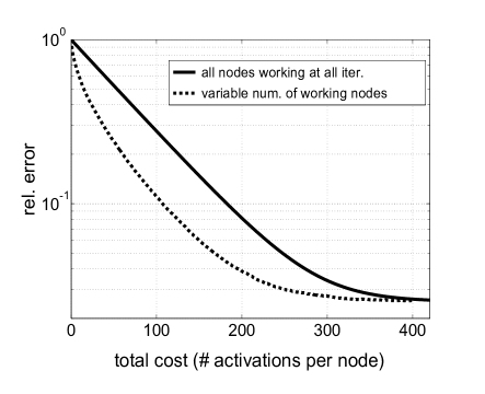
(a)  

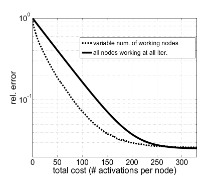
(b)  

Figure 1: Relative error versus total cost (number of activations per node) for quadratic costs and $n=100$-node network; Figure (a): $\Lambda_{i}^{k}=0$; Figure (b): $\Lambda_{i}^{k}=-I$. The solid lines correspond to all nodes working at all iterations; the dashed lines correspond to the method with idling (increasing number of working nodes).

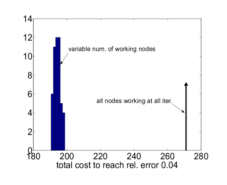
(a)  

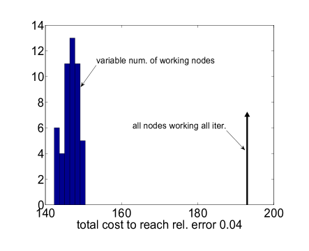
(b)  

Figure 2: Total cost (number of activations per node) to reach relative error $0.04$ for quadratic costs and $n=100$-node network; Figure (a): $\Lambda_{i}^{k}=0$; Figure (b): $\Lambda_{i}^{k}=-I$. The histograms corresponds to the DQN algorithm with idling; the arrow indicates the total cost needed by standard DQN.

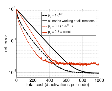
(a)  

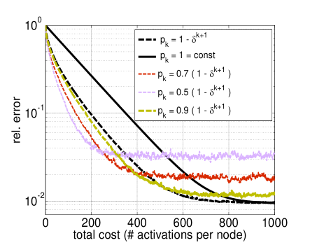
(b)  

Figure 3: Relative error versus total cost (number of activations per node) for strongly convex quadratic costs, $n=40$-node network, and $\Lambda_{i}^{k}=0$. The Figures compare the following scenarios: 1) $p_{k}\equiv 1$ (standard DQN); 2) $p_{k}=1-\sigma^{k+1}$; 3) $p_{k}=p_{\mathrm{max}}\left(1-\sigma^{k+1}\right)$; and 4) $p_{k}=p_{\mathrm{max}}$, for all $k$.

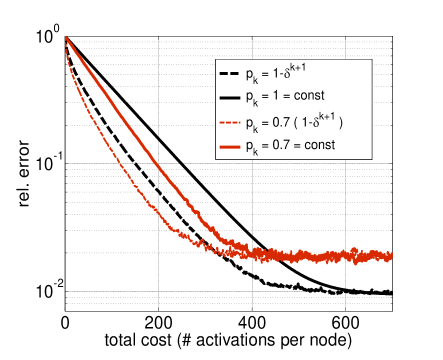
(a)  

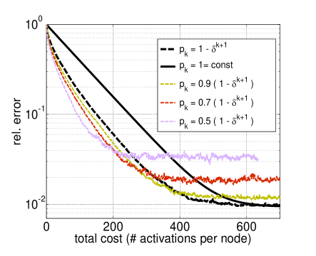
(b)  

Figure 4: Relative error versus total cost (number of activations per node) for strongly convex quadratic costs, $n=40$-node network, and $\Lambda_{i}^{k}=-I$. The Figures compare the following scenarios: 1) $p_{k}\equiv 1$ (standard DQN); 2) $p_{k}=1-\sigma^{k+1}$; 3) $p_{k}=p_{\mathrm{max}}\left(1-\sigma^{k+1}\right)$; and 4) $p_{k}=p_{\mathrm{max}}$, for all $k$.

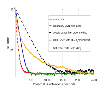
(a)  

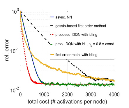
(b)  

Figure 5: Relative error versus total cost (number of activations per node) for strongly convex quadratic costs and $n=30$-node network and $\alpha=1/(100\,L)$ (top) and $\alpha=1/(100\,L)$ (bottom). The red, dotted line corresponds to the proposed DQN with idling and $p_{k}=1-\sigma^{k+1}$; the yellow, solid line to the method in [8] with $p_{k}=1-((1-\alpha\,\mu)^{2})^{k+1}$; blue, solid line to [17]; green, dashed line to the proposed DQN with idling and $p_{k}=0.8=\mathrm{const}$; and black, dashed line to the method in [29].

We consider the problem with strongly convex local quadratic costs; that is, for each $i=1,...,n$, we let $f_{i}:\,{\mathbb{R}}^{p}\rightarrow\mathbb{R}$, $f_{i}(x)=\frac{1}{2}(x-b_{i})^{T}A_{i}(x-b_{i})$, $p=10$, where $b_{i}\in{\mathbb{R}}^{p}$ and $A_{i}\in{\mathbb{R}}^{p\times p}$ is a symmetric positive definite matrix. The data pairs $A_{i},b_{i}$ are generated at random, independently across nodes, as follows. Each $b_{i}$’s entry is generated mutually independently from the uniform distribution on $[1,31]$. Each $B_{i}$ is generated as $B_{i}=Q_{i}\,D_{i}\,Q_{i}^{T}$; here, $Q_{i}$ is the matrix of orthonormal eigenvectors of $\frac{1}{2}(\widehat{B}_{i}+\widehat{B}_{i}^{T})$, and $\widehat{B}_{i}$ is a matrix with independent, identically distributed (i.i.d.) standard Gaussian entries; and $D_{i}$ is a diagonal matrix with the diagonal entries drawn in an i.i.d. fashion from the uniform distribution on $[1,31]$.

The network is a $n=100$-node instance of the random geometric graph model with the communication radius $r=\sqrt{\frac{\mathrm{ln}(n)}{n}}$, and it is connected. The weight matrix $W$ is set as follows: for $\{i,j\}\in E$, $i\neq j$, $w_{ij}=\frac{1}{2(1+\max\{d_{i},d_{j}\})}$, where $d_{i}$ is the node $i$’s degree; for $\{i,j\}\notin E$, $i\neq j$, $w_{ij}=0$; and $w_{ii}=1-\sum_{j\neq i}w_{ij}$, for all $i=1,...,n$.

We compare the standard DQN method and the DQN method with incorporated idling mechanism. Specifically, we study how the relative error (averaged across nodes):

$$\frac{1}{n}\sum_{i=1}^{n}\frac{\|x_{i}-\overline{x}^{*}\|}{\|\overline{x}^{*}\|},\,\,\overline{x}^{*}\neq 0,$$

evolves with the elapsed total number of activations per node. Note that the number of activations relates directly to both the communication and computational costs of the algorithm.

The parameters for both algorithms are set in the same way, and the only difference is in the activation schedule. For the method with idling, we set $p_{k}=1-\sigma^{k+1}$, $k=0,1,...$ We set $\sigma=1-c\,\alpha\,\mu$, with $c=40$. (Clearly, for the method without idling, $p_{k}\equiv 1$, for all $k$.) The remaining algorithm parameters are as follows. We set $\alpha=1/(100\,L)$, where $L$ is the Lipschitz constant of the gradients of the $f_{i}$’s that we take as $\max_{i=1,...,n}\|A_{i}\|$. Further, we let $\theta=0$, and $\epsilon=1$ (full step size). We consider two choices for $\Lambda_{i}^{k}$ in step 6 of Algorithm 3: $\Lambda_{i}^{k}=0$, for all $i,k$; and $\Lambda_{i}^{k}=-I$, for all $i,k$. (We apply no safeguarding on the above choices of $\Lambda_{i}^{k}$, i.e., we let $\rho=1$.) Note that the former choice corresponds to the algorithms with a single communication round per iteration $k$, while the latter corresponds to the algorithms with two communication rounds per $k$.

Figure 1 (a) plots the relative error versus total cost (equal to total number of activations per node up to the current iteration) for one sample path realization, for $\Lambda_{i}^{k}=0$. We can see that incorporating the idling mechanism significantly improves the efficiency of the algorithm: for the method to achieve the limiting accuracy of approximately $0.025$, the method without idling takes about $410$ activations per node, while the method with idling takes about $310$ activations. Hence, the idling mechanism reduces total cost by approximately $24\%$. Figure 1 (b) repeats the plots for $\Lambda_{i}^{k}=-I$, still showing clear gains of idling, though smaller than with $\Lambda_{i}^{k}=0$.

To account for randomness of the DQN method with idling that arises due to the random nodes’ activation schedule, we include histograms of the total cost needed to achieve a fixed level of relative error. Specifically, in Figure 2 we plot histograms of the total cost (corresponding to $50$ generated sample paths – $50$ different realizations of the $\xi_{i}^{k}$’s along iterations) needed to reach the relative error equal $0.04$; Figure 2 (a) corresponds to $\Lambda_{i}^{k}=0$, while Figure 2 (b) corresponds to $\Lambda_{i}^{k}=-I$. The Figures also indicate with arrows the total cost needed by standard DQN to achieve the same accuracy. The results confirm the gains of idling. Also, the variability of total cost across different sample paths is small relative to the gain with respect to standard DQN.

Figures 3 and 4 investigate the scenarios when the activation probability $p_{k}$ may not asymptotically converge to one. The network is a (connected) random geometric graph instance with $n=40$ and $r=\sqrt{\frac{\mathrm{ln}(n)}{n}}$; step size $\alpha=1/(200L)$; the remaining system and algorithmic parameters are the same as with the previous simulation example. We consider the following choices for $p_{k}$: 1) $p_{k}\equiv 1$ (standard DQN); 2) $p_{k}=1-\sigma^{k+1}$; 3) $p_{k}=p_{\mathrm{max}}\left(1-\sigma^{k+1}\right)$; and 4) $p_{k}=p_{\mathrm{max}}$, for all $k$. With the third and fourth choices, the presence of $p_{\mathrm{max}}$ models external effects on the $p_{k}$ (out of control of the networked nodes), e.g., due to link failures and unavailability of computing resources at certain iterations; it is varied within the set $\{0.5,0.7,0.9\}$. Figure 3 (a) compares the methods for one sample path realization with the four choices of $p_{k}$ above, with $p_{\mathrm{max}}=0.7$, for ${\Lambda_{i}^{k}}=0$. Figure 3 (b) compares for the same experiment the standard DQN ($p_{k}\equiv 1$), $p_{k}=1-\sigma^{k+1}$, and $p_{k}=p_{\mathrm{max}}\left(1-\sigma^{k+1}\right)$, with $p_{\mathrm{max}}\in\{0.5,0.7,0.9\}$. Several important observations stand out from the experiments. First, we can see that the limiting error increases when $p_{k}$ does not converge to one with respect to the case when it converges to one. However, this increase (deterioration) is moderate, and the algorithm still manages to converge to a good solution neighborhood despite the persisting idling. In particular, from Figure 3 (b), we can see that the limiting relative error increases from about $10^{-2}$ (with $p_{k}\rightarrow 1$) to about $3.5\cdot 10^{-2}$ with $p_{\mathrm{max}}=0.5$–a case with a strong persisting idling. This corroborates that DQN with idling is an effective method even when activation probability $p_{k}$ is not in full control of the algorithm designer. Second, the limiting error decreases when $p_{\mathrm{max}}$ increases, as it is expected – see Figure 3 (b). Finally, from Figure 3 (a), we can see that the method with $p_{k}=p_{\mathrm{max}}\left(1-\sigma^{k+1}\right)$ performs significantly better than the method with $p_{k}=p_{\mathrm{max}}$, for all $k$. In particular, the methods have the same limiting error (approximately $2\cdot 10^{-2}$), while the former approaches this error much faster. This confirms that the proposed judicious design of increasing $p_{k}$’s, as opposed to just keeping them constant, significantly improves the algorithm performance. Figure 4 repeats the same experiment for ${\Lambda_{i}^{k}}=-I$. We can see that the analogous conclusions can be drawn.

In the next experiment, we compare the proposed DQN method with idling with other existing methods that utilize randomized activations of nodes. Specifically, we consider the very recent asynchronous (second order) network Newton method proposed in [17] that is an asynchronous version of the method in [4]. We refer to this method here as asynchronous Network Newton (NN). We also consider the first order method with idling proposed in [8], and the first order gossip-based method in [29]. The method in [17] and the DQN with idling and matrix $\mathbb{L}=-I$ both utilize two $p$-dimensional communications per node activation (they have equal communication cost per node activation). The two methods also have a similar computational cost per activation. The method in [29] has a twice cheaper communication cost per activation, and it has in general a lower computational cost per activation (due to incorporating only the first order information into updates).

The comparison is carried out on a $n=30$-node (connected) random geometric graph instance with $91$ links, for the variable dimension $p=5$ and strongly convex quadratic $f_{i}$’s generated analogously to the previous experiments. With the proposed idling-DQN, we consider two choices of activation probabilities: 1) $p_{k}=1-\sigma^{k+1}$, with $\sigma=1-c\,\alpha\,\mu$, $c=40$, as in the previous experiment; and 2) $p_{k}=0.8=\mathrm{const}$. With [8], we let the activation probability $p_{k}=1-((1-\alpha\,\mu)^{2})^{k+1}$. The weight matrices of the proposed method and that in [17, 8] are set in the same way, as in prior experiments. With both idling-DQN and the method in [17], we set step size $\epsilon=1$. We consider two different choices of parameter $\alpha$: $\alpha=1/(100\,L)$, and $\alpha=1/(200\,L)$. This is how step-sizes are set for the method in [17] and for the idling-DQN with $p_{k}=1-\sigma^{k+1}$. Quantity $\alpha$ for the method in [29] (the algorithm’s step size) and for the idling-DQN with $p_{k}=0.8$ are then adjusted (decreased) for a fair comparison, so that the four different methods achieve the same asymptotic relative error; we then look how many per-node activations each method takes to reach the saturating relative error.

Figure 5 plots the relative error versus total number of activations for the four methods; Figure (a) corresponds to $\alpha=1/(100\,L)$ and Figure (b) is for $\alpha=1/(200\,L)$. We can see from Figure 5 (a) that the proposed idling-DQN with $p_{k}=1-\sigma^{k+1}$ outperforms the other methods: it takes about 400 per-node activations to reach the relative error $0.025$; the method in [17] and the idling-DQN with $p_{k}=0.8$ take about 600; and the method in [29] needs at least 1600 activations for the same accuracy. Note that, even when we half the number of activations for [29] to account for its twice cheaper communication cost, the proposed idling-DQN is still significantly faster – it compares versus [29] as 400 versus 800 “normalized activations.” DQN with idling outperforms the method in [8] in terms of the number of activations, while it is to be noted that [8] has a lower computational cost per activation. Interestingly, the idling DQN with constant $p_{k}$ and the method in [17] practically match in performance. Figure 5 (b) repeats the comparison for $\alpha=1/(200\,L)$; we can see that similar conclusions can be drawn from this experiment. In summary, the idling-DQN reduces communication cost with respect to the method in [29], which is expected as it utilizes more (second order) computations at each activation. The two second order methods with randomized activations, the idling-DQN and the method in [17], exhibit very similar performance when the idling-DQN uses constant $p_{k}$ policy. With the increasing $p_{k}$ policy, the idling-DQN performs better than [17]. This, together with previous experiments, demonstrates that a carefully designed workload orchestration with idling-DQN leads to performance improvements both with respect to a “pure” random activation policy and with respect to the all-nodes-work-all-time policy.

VII Conclusion

We incorporated an idling mechanism, recently proposed in the context of distributed first order methods [8], into distributed second order methods. Specifically, we study the DQN algorithm [10] with idling. We showed that, as long as $p_{k}$ converges to one at least as fast as $1/k^{1+\zeta}$, $\zeta>0$ arbitrarily small, the DQN algorithm with idling converges in the mean square sense and almost surely to the same point as the standard DQN method that activates all nodes at all iterations. Furthermore, when $p_{k}$ grows to one at a geometric rate, DQN with idling converges at a R-linear rate in the mean square sense. Therefore, DQN with idling achieves the same order of convergence (R-linear) as standard DQN, but with significantly cheaper iterations. Simulation examples corroborate communication and computational savings incurred by incorporating the idling mechanism and show the method’s flexibility with respect to the choice of activation probabilities.

The proposed idling-DQN method, and also other existing distributed second order methods (involving local Hessian’s computations) with randomized nodes’ activations, e.g., [17, 12], are not exact in the sense that they converge to a solution neighborhood. An interesting future research direction is to develop and analyze an idling-based second order method with exact convergence.

References

- [1] A. Nedić, A. Ozdaglar, “Distributed subgradient methods for multi-agent optimization,” IEEE Transactions on Automatic Control, vol. 54, no. 1, pp. 48–61, 2009.
- [2] F. Cattivelli, A. H. Sayed, “Diffusion LMS strategies for distributed estimation,” IEEE Transactions on Signal Processing, vol. 58, no. 3, pp. 1035–1048, 2010.
- [3] W. Shi, Q. Ling, G. Wu, W. Yin, “EXTRA: an Exact First-Order Algorithm for Decentralized Consensus Optimization,” SIAM Journal on Optimization, vol. 2, no. 25, pp. 944-966, 2015.
- [4] A. Mokhtari, Q. Ling, A. Ribeiro, “Network Newton Distributed Optimization Methods,” IEEE Trans. Signal Processing, vol. 65, no. 1, pp. 146-161, 2017.
- [5] L. Xiao, S. Boyd, S. Lall, “A scheme for robust distributed sensor fusion based on average consensus,” in IPSN ’05, Information Processing in Sensor Networks, 63–70, Los Angeles, California, 2005.
- [6] G. Hug, S. Kar, C. Wu, “Consensus + Innovations Approach for Distributed Multiagent Coordination in a Microgrid,” IEEE Trans. Smart Grid, vol. 6, no. 4, pp. 1893-1903, 2015.
- [7] F. Bullo, J. Cortes, S. Mart nez, “Distributed Control of Robotic Networks: A Mathematical Approach to Motion Coordination Algorithms,” Princeton University Press, 2009.
- [8] D. Bajović, D. Jakovetić, N. Krejić, N. Krklec Jerinkić, “Distributed Gradient Methods with Variable Number of Working Nodes,” IEEE Trans. Signal Processing, vol. 64, no. 15, pp. 4080-4095, 2016.
- [9] M. P. Friedlander, M. Schmidt, “Hybrid deterministic-stochastic methods for data fitting,” SIAM Journal on Scientific Computing, vol. 34, pp. 1380-1405, 2012.
- [10] D. Bajović, D. Jakovetić, N. Krejić, N. Krklec Jerinkić, “Newton-like method with diagonal correction for distributed optimization,” SIAM J. Opt., vol. 27, no. 2, pp. 1171 1203. 2017.
- [11] D. Varagnolo, F. Zanella, A. Cenedese, G. Pillonetto, and L. Schenato, “Newton-Raphson Consensus for Distributed Convex Optimization,” IEEE Trans. Aut. Contr., vol. 61, no. 4, 2016.
- [12] M. Eisen, A. Mokhtari, A. Ribeiro, “Decentralized quasi-Newton methods,” IEEE Transactions on Signal Processing, vol. 65, no. 10, pp. 2613–2628, May 2017.
- [13] M. Eisen, A. Mokhtari, A. Ribeiro, “A Decentralized Quasi-Newton Method for Dual Formulations of Consensus Optimization,” IEEE 55th Conference on Decision and Control (CDC), Las Vegas, NV, Dec. 2016.
- [14] M. Eisen, A. Mokhtari, A. Ribeiro, “An asynchronous quasi-Newton method for consensus optimization,” IEEE Global Conference on Signal and Information Processing (GlobalSIP), Washington, DC, VA, USA, Dec. 2016.
- [15] D. Bajović, D. Jakovetić, N. Krejić, N. Krklec Jerinkić, “Distributed first and second order methods with variable number of working nodes,” IEEE Global Conference on Signal and Information Processing, Washington DC, VA, USA, Dec. 2016
- [16] A. Mokhtari, W. Shi, Q. Ling, A. Ribeiro, “DQM: Decentralized Quadratically Approximated Alternating Direction Method of Multipliers,” IEEE Trans. Signal Processing, vol. 64, no. 19, pp. 5158-5173, 2016.
- [17] F. Mansoori, E. Wei, “Superlinearly Convergent Asynchronous Distributed Network Newton Method,” 2017, available at https://arxiv.org/abs/1705.03952
- [18] D. Jakovetić, J. M. F. Moura, J. Xavier, “Distributed Nesterov-like gradient algorithms”, CDC’12, 51 IEEE Conference on Decision and Control, Maui, Hawaii, December 2012, pp. 5459–5464.
- [19] A. Mokhtari, W. Shi, Q. Ling, A. Ribeiro, “A Decentralized Second Order Method with Exact Linear Convergence Rate for Consensus Optimization,” IEEE Trans. Signal and Information Processing over Networks, vol. 2, no. 4. pp. 507-522, 2016.
- [20] M. Zargham, A. Ribeiro, A. Jadbabaie, “Accelerated dual descent for constrained convex network flow optimization,” Decision and Control (CDC), 2013 IEEE 52nd Annual Conference on, Firenze, Italy, 2013. pp. 1037-1042.
- [21] I. Lobel, A. Ozdaglar, D. Feijer, “Distributed Multi-agent Optimization with State-Dependent Communication,” Mathematical Programming, vol. 129, no. 2, pp. 255-284, 2014.
- [22] X. Zhao, A. H. Sayed, “Asynchronous Adaptation and Learning Over Networks –Part I: Modeling and Stability Analysis,” IEEE Transactions on Signal Processing, vol. 63, no. 4, Feb. 2015.
- [23] X. Zhao, A. H. Sayed, “Asynchronous Adaptation and Learning Over Networks –Part II: Performance Analysis,” IEEE Transactions on Signal Processing, vol. 63, no. 4, Feb. 2015.
- [24] T. Wu, K. Yuan, Q. Ling, W. Yin, A. H, Sayed, “Decentralized Consensus Optimization with Asynchrony and Delays,” IEEE Transactions on Signal and Information Processing over Networks, to appear, 2017, DOI: 10.1109/TSIPN.2017.2695121
- [25] J. Liu, S. Wright, “Asynchronous stochastic coordinate descent: Parallelism and convergence properties,” SIAM J. Opt., vol. 25, no. 1, 2015.
- [26] T. H. Chang, L. Wei-Cheng, M. Hong, X. Wang, “Distributed ADMM for large-scale optimization part II: Linear convergence analysis and numerical performance,” IEEE Trans. Sig. Proc., vol. 64, no. 12, 2016.
- [27] N. Krejić, N. Krklec Jerinkić, “Nonmonotone line search methods with variable sample size,” Numerical Algorithms, vol. 68, pp. 711–739, 2015.
- [28] S. Ram, A. Nedic, V. Veeravalli, “Distributed stochastic subgradient projection algorithms for convex optimization,” J. Optim. Theory Appl., vol. 147, no. 3, pp. 516 -545, 2011.
- [29] S. S. Ram, A. Nedić, V. Veeravalli, “Asynchronous gossip algorithms for stochastic optimization,” CDC ’09, 48th IEEE International Conference on Decision and Control, Shanghai, China, December 2009, pp. 3581 – 3586.
- [30] E. Wei, A. Ozdaglar, A. Jadbabaie, “A distributed Newton method for network utility maximization –I: Algorithm,” IEEE Transactions on Automatic Control, vol. 58, no. 9, pp. 2162- 2175, 2013.