Boosting the kernelized shapelets:
Theory and algorithms for local features

Abstract

We consider binary classification problems using local features of objects. One of motivating applications is time-series classification, where features reflecting some local closeness measure between a time series and a pattern sequence called shapelet are useful. Despite the empirical success of such approaches using local features, the generalization ability of resulting hypotheses is not fully understood and previous work relies on a bunch of heuristics. In this paper, we formulate a class of hypotheses using local features, where the richness of features is controlled by kernels. We derive generalization bounds of sparse ensembles over the class which is exponentially better than a standard analysis in terms of the number of possible local features. The resulting optimization problem is well suited to the boosting approach and the weak learning problem is formulated as a DC program, for which practical algorithms exist. In preliminary experiments on time-series data sets, our method achieves competitive accuracy with the state-of-the-art algorithms with small parameter-tuning cost.

1 Introduction

Classifying objects using their “local” patterns is often effective in various applications. For example, in time-series classification problems, a local feature called shapelet is shown to be quite powerful in the data mining literature (Ye and Keogh, 2009; Keogh and Rakthanmanon, 2013; Hills et al., 2014; Grabocka et al., 2014). More precisely, a shapelet ${\bf z}=(z_{1},\dots,z_{\ell})$ is a real-valued “short” sequence in $\mathbb{R}^{\ell}$ for some $\ell>1$. Given a time-series ${\bf x}=(x_{1},\dots,x_{L})$, a typical measure of closeness between the time-series ${\bf x}$ and the shapelet ${\bf z}$ is $\min_{j=1}^{Q}\|{\bf x}_{j:j+\ell-1}-{\bf z}\|_{2}$, where $Q=L-\ell+1$ and ${\bf x}_{j:j+\ell-1}=(x_{j},\dots,x_{j+\ell-1})$. Here, the measure focuses on “local” closeness between the time-series and the shapelet. In many time-series classification problems, sparse combinations of features based on the closeness to some shapelets are useful (Grabocka et al., 2015; Renard et al., 2015; Hou et al., 2016). Similar situations could happen in other applications. Say, for image classification problems, template matching is a well-known technique to measure similarity between an image and “(small) template image” in a local sense.

Despite the empirical success of applying local features, theoretical guarantees of such approaches are not fully investigated. In particular, trade-offs of the richness of such local features and the generalization ability are not characterized yet.

In this paper, we formalize a class of hypotheses based on some local closeness. Here, the richness of the class is controlled by associated kernels. We show generalization bounds of ensembles of such local classifiers. Our bounds are exponentially tighter in terms of some parameter than typical bounds obtained by a standard analysis.

Further, for learning ensembles of the kernelized hypotheses, our theoretical analysis suggests a $1$-norm constrained optimization problem with infinitely many parameters, for which the dual problem is categorized as a semi-infinite program (see Shapiro, 2009). To obtain approximate solutions of the problem efficiently, we take the approach of boosting (Schapire et al., 1998). In particular, we employ LPBoost (Demiriz et al., 2002), which solve $1$-norm constrained soft margin optimization via a column generation approach. As a result, our approach has two stages, where the master problem is a linear program and the sub-problems are difference of convex programs (DC programs), which are non-convex. While it is difficult to solve the sub-problems exactly due to non-convexity, various techniques are investigated for DC programs and we can find good approximate solutions efficiently for many cases in practice.

In preliminary experiments on time-series data sets, our method achieves competitive accuracy with the state-of-the-art algorithms using shapelets. While the previous algorithms need careful parameter tuning and heuristics, our method uses less parameter tuning and parameters can be determined in an organized way. In addition, our solutions tend to be sparse and could be useful for domain experts to select good local features.

1.1 Related work

The concept of time-series shapelets was first introduced by Ye and Keogh (2009). The algorithm finds shapelets by using the information gains of potential candidates associated with all the subsequences of the given time series and constructs a decision tree. Shapelet transform (Hills et al., 2014) is a technique combining with shapelets and machine learning. The authors consider the time-series examples as feature vectors defined by the set of local closeness to some shapelets and in order to obtain classification rule, they employed some effective learning algorithms such as linear SVM or random forests. Note that shapelet transform completely separate the phase searching for shapelets from the phases of creating classification rules. Afterward, many algorithms have been proposed to search the good shapelets efficiently keeping high prediction accuracy in practice (Keogh and Rakthanmanon, 2013; Grabocka et al., 2015; Renard et al., 2015; Karlsson et al., 2016). The algorithms are based on the idea that discriminative shapelets are contained in the training data. This approach, however, might overfit without a regularization. Learning Time-Series Shapelets (LTS) algorithm (Grabocka et al., 2014) is a different approach from such subsequence-based algorithms. LTS approximately solves an optimization problem of learning the best shapelets directly without searching subsequences in a brute-force way. In contrast to the above subsequence-based methods, LTS finds nearly optimal shapelets and achieves higher prediction accuracy than the other existing methods in practice. However, there is no theoretical guarantee of its generalization error.

There are previous results using local features based on kernels  (e.g., Odone et al., 2005; Harris, ; Shimodaira et al., 2001; Zhang et al., 2010). However, their approaches focus on the closeness (similarity) between examples (e.g., subsequence $a$ of example $A$ and subsequence $b$ of example $B$), not known to capture local similarity.

2 Preliminaries

Let $\mathcal{P}\subseteq\mathbb{R}^{\ell}$ be a set, in which an element is called a pattern. Our instance space $\mathcal{X}$ is a set of sequences of patterns in $\mathcal{P}$. For simplicity, we assume that every sequence in $\mathcal{X}$ is of the same length. That is, $\mathcal{X}\subseteq\mathcal{P}^{Q}$ for some integer $Q$. We denote by ${\bf x}=({\bf x}^{(1)},\ldots,{\bf x}^{(Q)})$ an instance sequence in $\mathcal{X}$, where every ${\bf x}^{(j)}$ is a pattern in $\mathcal{P}$. The learner receives a labeled sample $S=((({\bf x}_{1}^{(1)},\ldots,{\bf x}_{1}^{(Q)}),y_{1}),\ldots,(({\bf x}_{m}^{(1)},\ldots,{\bf x}_{m}^{(Q)}),y_{m}))\in(\mathcal{X}\times\{-1,1\})^{m}$ of size $m$, where each labeled instance is independently drawn according to some unknown distribution $D$ over $\mathcal{X}\times\{-1,+1\}$.

Let $K$ be a kernel over $\mathcal{P}$, which is used to measure the similarity between patterns, and let $\Phi:\mathcal{P}\to\mathbb{H}$ denote a feature map associated with the kernel $K$ for a Hilbert space $\mathbb{H}$. That is, $K({\bf z},{\bf z}^{\prime})=\langle\Phi({\bf z}),\Phi({\bf z}^{\prime})\rangle$ for patterns ${\bf z},{\bf z}^{\prime}\in\mathcal{P}$, where $\langle\cdot,\cdot\rangle$ denotes the inner product over $\mathbb{H}$. The norm induced by the inner product is denoted by $\|\cdot\|_{\mathbb{H}}$ and satisfies $\|{\bf u}\|_{\mathbb{H}}=\sqrt{\langle{\bf u},{\bf u}\rangle}$ for ${\bf u}\in\mathbb{H}$.

For each ${\bf u}\in\mathbb{H}$, we define the base classifier (or the feature), denoted by $h_{{\bf u}}$, as the function that maps a given sequence ${\bf x}=({\bf x}^{(1)},\ldots,{\bf x}^{(Q)})\in\mathcal{X}$ to the maximum of the similarity scores between ${\bf u}$ and ${\bf x}^{(j)}$ over all patterns ${\bf x}^{(j)}$ in ${\bf x}$. More specifically,

$$h_{{\bf u}}({\bf x})=\max_{j\in[Q]}\left\langle{\bf u},\Phi({\bf x}^{(j)})\right\rangle,$$

where $[Q]$ denotes the set $\{1,2,\ldots,Q\}$. For a set $U\subseteq\mathbb{H}$, we define the class of base classifiers as

$$H_{U}=\left\{h_{{\bf u}}\mid{\bf u}\in U\right\}$$

and we denote by $\mathrm{conv}(H_{U})$ the set of convex combinations of base classifiers in $H_{U}$. More precisely,

$$\mathrm{conv}(H_{U})=\left\{\sum_{{\bf u}\in U^{\prime}}w_{\bf u}h_{\bf u}({\bf x})\mid\forall{\bf u}\in U^{\prime},w_{\bf u}\geq 0,\sum_{{\bf u}\in U^{\prime}}w_{\bf u}=1,\text{$U^{\prime}\subseteq U$ is a finite support}\right\}.$$

The goal of the learner is to find a final hypothesis $g\in\mathrm{conv}(H_{U})$, so that its generalization error $\mathcal{E}_{D}(g)=\Pr_{({\bf x},y)\sim D}[\mathrm{sign}(g({\bf x}))\neq y]$ is small.

Example: Learning with time-series shapelets

For a typical setting of learning with time-series shapelets, an instance is a sequence of real numbers ${\bf x}=(x_{1},x_{2},\ldots,x_{L})\in\mathbb{R}^{L}$ and a base classifier $h_{\bf s}$, which is associated with a shapelet (i.e., a “short” sequence of real numbers) ${\bf s}=(s_{1},s_{2},\ldots,s_{\ell})\in\mathbb{R}^{\ell}$, is defined as

$$h_{\bf s}({\bf x})=\max_{1\leq j\leq L-\ell+1}K({\bf s},{\bf x}^{(j)}),$$

where ${\bf x}^{(j)}=(x_{j},x_{j+1},\ldots,x_{j+\ell})$ is the subsequence of ${\bf x}$ of length $\ell$ that begins with $j$th index. In our framework, this corresponds to the case where $Q=L-\ell+1$, $\mathcal{P}\subseteq\mathbb{R}^{\ell}$, and $U=\{\Phi({\bf s})\mid{\bf s}\in\mathcal{P}\}$.

3 Risk bounds of the hypothesis classes

In this section, we give generalization bounds of the hypothesis classes $\mathrm{conv}(H_{U})$ for various $U$ and $K$. To derive the bounds, we use the Rademacher and the Gaussian complexity (Bartlett and Mendelson, 2003).

Definition 1

(The Rademacher and the Gaussian complexity, Bartlett and Mendelson, 2003) Given a sample $S=({\bf x}_{1},\dots,{\bf x}_{m})\in\mathcal{X}^{m}$, the empirical Rademacher complexity $\mathfrak{R}(H)$ of a class $H\subset\{h:\mathcal{X}\to\mathbb{R}\}$ w.r.t. $S$ is defined as $\mathfrak{R}_{S}(H)=\frac{1}{m}\mathop{\rm E}\limits_{\boldsymbol{\sigma}}\left[\sup_{h\in H}\sum_{i=1}^{m}\sigma_{i}h({\bf x}_{i})\right]$, where $\boldsymbol{\sigma}\in\{-1,1\}^{m}$ and each $\sigma_{i}$ is an independent uniform random variable in $\{-1,1\}$. The empirical Gaussian complexity $\mathfrak{G}_{S}(H)$ of $H$ w.r.t. $S$ is defined similarly but each $\sigma_{i}$ is drawn independently from the standard normal distribution.

The following bounds are well-known.

Lemma 1

(Bartlett and Mendelson, 2003, Lemma 4) $\mathfrak{R}_{S}(H)=O(\mathfrak{G}_{S}(H))$.

Lemma 2

(Mohri et al., 2012, Corollary 6.1) For fixed $\rho$, $\delta>0$, the following bound holds with probability at least $1-\delta$: for all $f\in\mathrm{conv}(H)$,

$$\mathcal{E}_{D}(f)\leq\mathcal{E}_{S,\rho}(f)+\frac{2}{\rho}\mathfrak{R}_{S}(H)+3\sqrt{\frac{\log\frac{1}{\delta}}{2m}},$$

where $\mathcal{E}_{S,\rho}(f)$ is the empirical margin loss of $f$ over $S$, i.e., the ratio of examples for which $f$ has margin $y_{i}f({\bf x}_{i})<\rho$.

To derive generalization bounds based on the Rademacher or the Gaussian complexity is quite standard in the statistical learning theory literature and applicable to our classes of interest as well. However, a standard analysis provides us sub-optimal bounds.

For example, let us consider the simple case where the class $H_{U}$ of base classifiers is defined by the linear kernel with $U$ to be the set of vectors in $\mathbb{R}^{\ell}$ of bounded norm. In this case, $H_{U}$ can be viewed as $H_{U}=\{\max\{h_{1},\dots,h_{Q}\}\mid h_{1}\in H_{1},\ldots,h_{Q}\in H_{Q}\}$, where $H_{j}=\{h:{\bf x}\mapsto\langle{\bf u},{\bf x}^{(j)}\rangle\mid{\bf u}\in U\}$ for every $j\in[Q]$. Then, by a standard analysis  (see, e.g., Mohri et al., 2012, Lemma 8.1), we have $\mathfrak{R}(H_{U})\leq\sum_{j=1}^{Q}\mathfrak{R}(H_{j})=O\left(\frac{Q}{\sqrt{m}}\right)$. However, this bound is weak since it is linear in $Q$. In the following, we will give an improved bound of $\tilde{O}(\log Q/\sqrt{m})$. The key observation is that if base classes $H_{1},\dots,H_{Q}$ are “correlated” somehow, one could obtain better Rademacher bounds. In fact, we will exploit some geometric properties among these base classes.

3.1 Main theorem

First, we show our main theoretical result on the generalization bound of $\mathrm{conv}(H_{U})$.

Given a sample $S$, let $\mathcal{P}_{S}$ be the set of patterns appearing in $S$ and let $\Phi(\mathcal{P}_{S})=\{\Phi({\bf z})\mid{\bf z}\in\mathcal{P}_{S}\}$. Let $\Phi_{\mathrm{diff}}(\mathcal{P}_{S})=\{\Phi({\bf z})-\Phi({\bf z}^{\prime})\mid{\bf z},{\bf z}^{\prime}\in\mathcal{P}_{S},{\bf z}\neq{\bf z}^{\prime}\}$. By viewing each instance ${\bf v}\in\Phi_{\mathrm{diff}}(\mathcal{P}_{S})$ as a hyperplane $\{{\bf u}\mid\langle{\bf v},{\bf u}\rangle=0\}$, we can naturally define a partition of the Hilbert space $\mathbb{H}$ by the set of all hyperplanes ${\bf v}\in\Phi_{\mathrm{diff}}(\mathcal{P}_{S})$. Let $\mathcal{I}$ be the set of all cells of the partition. Each cell $I\in\mathcal{I}$ is a polyhedron which is defined by a minimal set $V_{I}\subseteq\Phi_{\mathrm{diff}}(\mathcal{P}_{S})$ that satisfies $I=\bigcap_{{\bf v}\in V_{I}}\{{\bf u}\mid\langle{\bf u},{\bf v}\rangle\geq 0\}$. Let

$$\mu^{*}=\min_{I\in\mathcal{I}}\max_{{\bf u}\in I\cap U}\min_{{\bf v}\in V_{I}}|\langle{\bf u},{\bf v}\rangle|.$$

Let $d^{*}_{\Phi,S}$ be the VC dimension of the set of linear classifiers over the finite set $\Phi_{\mathrm{diff}}(\mathcal{P}_{S})$, given by $F_{U}=\{f:{\bf v}\mapsto\mathrm{sign}(\langle{\bf u},{\bf v}\rangle)\mid{\bf u}\in U\}$. Then, our main result is stated as follows:

Theorem 1

Suppose that for any ${\bf z}\in\mathcal{P}$, $\|\Phi({\bf z})\|_{\mathbb{H}}\leq R$. Then, for any $\rho>0$ and $\delta(0<\delta<1)$, with probability at least $1-\delta$, the following holds for any $g\in\mathrm{conv}(H_{U})$ with $U\subseteq\{{\bf u}\in\mathbb{H}\mid\|{\bf u}\|_{\mathbb{H}}\leq\Lambda\}$:

$$\mathcal{E}_{D}(g)\leq \mathcal{E}_{\rho}(g)+O\left(\frac{R\Lambda\sqrt{d_{\Phi,S}^{*}\log(mQ)}}{\rho\sqrt{m}}+\sqrt{\frac{\log\frac{1}{\delta}}{m}}\right).$$ (1)

In particular, (i) if $\Phi$ is the identity mapping (i.e., the associated kernel is the linear kernel), or (ii) if $\Phi$ satisfies that $\left\langle\Phi({\bf z}),\Phi({\bf x})\right\rangle$ is monotone decreasing with respect to $\|{\bf z}-{\bf x}\|_{2}$ (e.g., the mapping defined by the Gaussian kernel) and $U=\{\Phi({\bf s})\mid{\bf s}\in\mathbb{R}^{\ell},\|\Phi({\bf s})\|_{\mathbb{H}}\leq\Lambda\}$, then $d^{*}_{\Phi,S}$ can be replaced by $\ell$. (iii) Otherwise, $d^{*}_{\Phi,S}\leq R\Lambda/\mu^{*}$.

In order to prove the theorem 1, we show several definitions, lemmas and the proofs as following subsection.

3.2 Proof sketch

Definition 2

The set $\Theta$ of mappings from an instance to a pattern For any ${\bf u}\in U$, let $\theta_{\bf u}:[m]\to[Q]$ be a mapping defined by

$$\theta_{{\bf u}}(i):=\arg\max_{j\in[Q]}\left\langle{\bf u},\Phi\left({\bf x}_{i}^{(j)}\right)\right\rangle,$$

and we denote the set of all $\theta_{{\bf u}}$ as $\Theta=\{\theta_{{\bf u}}\mid{\bf u}\in U\}$.

Lemma 3

Suppose that for any ${\bf z}\in\mathcal{P}$, $\|\Phi({\bf z})\|_{\mathbb{H}}\leq R$. Then, the empirical Gaussian complexity of $H_{U}$ with respect to $S$ for $U\subseteq\{{\bf u}\mid\|{\bf u}\|_{\mathbb{H}}\leq\Lambda\}$ is bounded as follows:

$$\mathfrak{G}_{S}(H)\leq\frac{R\Lambda\sqrt{(\sqrt{2}-1)+2(\ln|\Theta|)}}{\sqrt{m}}.$$

The proof is given in the supplemental material.

Thus, it suffices to bound the size $|\Theta|$. Naively the size $|\Theta|$ is at most $Q^{m}$ since there are $Q^{m}$ possible mappings from $[m]$ to $[Q]$. However, this naive bound is too pessimistic. The basic idea to get better bounds is the following. Fix any $i\in[m]$ and consider points $\Phi({\bf x}_{i}^{1}),\dots,\Phi({\bf x}_{i}^{Q})$. Then, we define equivalence classes of ${\bf u}$ such that $\theta_{\bf u}(i)$ is the same, which define a Voronoi diagram for the points $\Phi({\bf x}_{i}^{1}),\dots,\Phi({\bf x}_{i}^{Q})$. Note here that the closeness is measured by the inner product, not a distance. More precisely, let $V_{i}=(V_{i}^{(1)},\dots,V_{i}^{(Q)})$ be the Voronoi diagram defined as $V_{i}^{(j)}=\{{\bf u}\in\mathbb{H}\mid\theta_{\bf u}(i)=j\}$. Let us consider the set of intersections $\cap_{i\in[m]}V_{i}^{(j_{i})}$ for all combinations of $(j_{1},\dots,j_{m})\in[Q]^{m}$. The key observation is that each non-empty intersection corresponds to a mapping $\theta\in\Theta$. Thus, we obtain $|\Theta|=(\text{the number of intersections $\cap_{i\in[m]}V_{i}^{(j_{i})}$})$. In other words, the size of $\Theta$ is exactly the number of rooms defined by the intersections of $m$ Voronoi diagrams $V_{1},\dots,V_{m}$. From now on, we will derive upper bounds based on this observation.

Lemma 4

$$|\Theta|=O((mQ)^{2d_{\Phi,S}^{*}}).$$

The proof is shown in the supplemental material.

Theorem 2

1. If $\Phi$ is the identity mapping over $\mathcal{P}$, then $|\Theta|=O((mQ)^{2\ell})$.

2. if $\Phi$ satisfies that $\left\langle\Phi({\bf z}),\Phi({\bf x})\right\rangle$ is monotone decreasing with respect to $\|{\bf z}-{\bf x}\|_{2}$ (e.g., the mapping defined by the Gaussian kernel) and $U=\{\Phi({\bf s})\mid{\bf s}\in\mathbb{R}^{\ell},\|\Phi({\bf s})\|_{\mathbb{H}}\leq\Lambda\}$, then $|\Theta|=O((mQ)^{2\ell})$.

3. Otherwise, $|\Theta|=O((mQ)^{R\Lambda/\mu^{*}})$.

The proof is shown in the supplemental material.

Now we are ready to prove Theorem 1.

Proof [Proof of Theorem 1] By using Lemma 1, and 2, we obtain the generalization bound in terms of the Gaussian complexity of $H$. Then, by applying Lemma 3 and Theorem 2, we complete the proof.  

4 Optimization problem formulation

In this section, we formulate an optimization problem to learn ensembles in $\mathrm{conv}(H_{U})$ for $U\subseteq\{{\bf u}:\|{\bf u}\|_{\mathbb{H}}\leq\Lambda\}$. The problem is a $1$-norm constrained soft margin optimization problem using hypotheses in $H_{U}$, which is a linear program.

$$\max\limits_{\rho,{\bf w},\boldsymbol{\xi}}\quad \rho-\frac{1}{\nu m}\sum_{i=1}^{m}\xi_{i}$$ (2)

sub.to $$\int_{{\bf u}\in U}y_{i}{\bf w}_{{\bf u}}h_{\bf u}({\bf x}_{i})d{\bf u}\geq\rho-\xi_{i},~{}i\in[m],\int_{{\bf u}\in U}w_{{\bf u}}d{\bf u}=1,{\bf w}\geq\boldsymbol{0},~{}\rho\in\mathbb{R},$$

where $h_{\bf u}\in H_{U}$ is a given base classifiers, $\nu\in[0,1]$ is a constant parameter, $\rho$ is a target margin and $\xi_{i}$ is a slack variable. The dual problem (2) is given as follows.

$$\min\limits_{\gamma,{\bf d}}\quad \gamma$$ (3)

sub.to $$\sum_{i=1}^{m}y_{i}d_{i}h_{\bf u}({\bf x}_{i})\leq\gamma,\quad{\bf u}\in U,~{}~{}0\leq d_{i}\leq 1/\nu m~{}(i\in[m]),~{}~{}\sum_{i=1}^{m}d_{i}=1,~{}\gamma\in\mathbb{R}.$$

The dual problem is categorized as a semi-infinite program (SIP), since it contains possibly infinitely many constraints. Note that the duality gap is zero since the problem (3) is convex and the optimum is finite (Shapiro, 2009, Theorem 2.2). Our approach is to approximately solve the primal and the dual problems for $U=\{{\bf u}:\|{\bf u}\|_{\mathbb{H}}\leq\Lambda\}$ by solving the sub-problems over a finite subset $U^{\prime}\subset U$. Such approach is called column generation in linear programming, which add a new constraint (column) to the dual problems and solve them iteratively. LPBoost (Demiriz et al., 2002) is a well known example of the approach in the boosting setting. At each iteration, LPBoost chooses a hypothesis $h_{\bf u}$ so that $h_{\bf u}$ maximally violates the constraints in the current dual problem. This sub-problem is called weak learning in the boosting setting and formulated as follows:

$$\max_{{\bf u}\in\mathbb{H}}\quad\sum_{i=1}^{m}y_{i}d_{i}\max_{j\in[Q]}\left\langle{\bf u},\Phi\left({\bf x}_{i}^{(j)}\right)\right\rangle\quad\text{sub.to}\quad\|{\bf u}\|_{\mathbb{H}}^{2}\leq\Lambda^{2}.$$ (4)

However, the problem (4) cannot be solved directly, since we have only access to $U$ though the associated kernel. Fortunately, the optimal solution ${\bf u}^{*}$ of the problem can be written as a linear combination of the functions $K({\bf x}_{i},\cdot)$ because of the following representer theorem.

Theorem 3 (Representer Theorem)

The optimal solution ${\bf u}^{*}$ of optimization problem (4) has the form of ${\bf u}^{*}=\sum_{i=1}^{m}\sum_{j=1}^{Q}\alpha_{ij}K({\bf x}_{i}^{(j)},\cdot)$.

The proof is shown in the supplemental material.

By Theorem 3, we can design a weak learner by solving the following equivalent problem:

$$\min_{\boldsymbol{\alpha}}-\sum_{p:y_{p}=+1}\hat{d}_{p}\max_{j\in[Q]}\sum_{i=1}^{m}\sum_{k=1}^{Q}\alpha_{ik}K\left({\bf x}_{i}^{(k)},{\bf x}_{p}^{(j)}\right)+\sum_{q:y_{q}=-1}\hat{d}_{q}\max_{j\in[Q]}\sum_{i=1}^{m}\sum_{k=1}^{Q}\alpha_{ik}K\left({\bf x}_{i}^{(k)},{\bf x}_{q}^{(j)}\right)$$ (5)

$$\text{sub.to}\quad\sum_{i,k}^{m}\sum_{j,l}^{Q}\alpha_{ij}\alpha_{kl}K\left({\bf x}_{i}^{(j)},{\bf x}_{k}^{(l)}\right)\leq\Lambda^{2}.$$

5 Algorithm

The optimization problem (5) is difference of convex functions (DC) programming problem and we can obtain local optimum $\epsilon$-approximately by using DC Algorithm (Tao and Souad, 1988). For the above optimization problem, we replace $\max_{j\in[Q]}\sum_{i=1}^{m}\sum_{k=1}^{Q}\alpha_{ik}K\left({\bf x}_{i}^{(k)},{\bf x}_{q}^{(j)}\right)$ with $\lambda_{q}$, then we get the equivalent optimization problem as below.

$$\min_{\boldsymbol{\alpha},\boldsymbol{\lambda}}\quad -\sum_{p:y_{p}=+1}\hat{d}_{p}\max_{j\in[Q]}\sum_{i=1}^{m}\sum_{k=1}^{Q}\alpha_{ik}K\left({\bf x}_{i}^{(k)},{\bf x}_{p}^{(j)}\right)+\sum_{q:y_{q}=-1}\hat{d}_{q}\lambda_{q}$$ (6)

sub.to $$\sum_{i=1}^{m}\sum_{k=1}^{Q}\alpha_{ik}K\left({\bf x}_{i}^{(k)},{\bf x}_{q}^{(j)}\right)\leq\lambda_{q}~{}(j\in[Q],\forall q:y_{q}=-1),~{}~{}$$

$$\sum_{i,k=1}^{m}\sum_{j,l=1}^{Q}\alpha_{ij}\alpha_{kl}K\left({\bf x}_{i}^{(j)},{\bf x}_{k}^{(l)}\right)\leq\Lambda^{2}.$$

We show the pseudo code of LPBoost using column generation algorithm, and our weak learning algorithm using DC programming in Algorithm 1 and 2, respectively. In Algorithm 2, the optimization problem (7) can be solved by standard QP solver.

Algorithm 1 LPBoost with WeakLearn

1. Input: $S$, $\Lambda$, $\epsilon>0$

2. Initialize: ${\bf d}_{0}\leftarrow(\frac{1}{m},\ldots,\frac{1}{m})$

3. For $t=1,\dots,T$

   1. $h_{t}\leftarrow$ Run WeakLearn($S$, ${\bf d}_{t-1}$, $\Lambda$, $\epsilon$)

   2. Solve optimization problem:

      $$(\gamma,{\bf d}_{t})\leftarrow\arg\min\limits_{\gamma,{\bf d}}\quad\gamma\quad\quad\quad$$

      $$\text{sub.to}~{}~{}\sum_{i=1}^{m}y_{i}d_{i}h_{j}({\bf x}_{i})\leq\gamma~{}~{}(j\in[t]),~{}~{}0\leq d_{i}\leq 1/\nu m~{}~{}(i\in[m]),\sum_{i=1}^{m}d_{i}=1,~{}\gamma\in\mathbb{R}.$$

4. ${\bf w}\leftarrow$ Lagrangian multipliers of solution of last optimization problem

5. $g\leftarrow\sum_{j=1}^{T}w_{j}h_{j}$

6. Output: $\mathrm{sign}(g)$

Algorithm 2 WeakLearn by DC Algorithm

1. Input: $S$, ${\bf d}$, $\Lambda$, $\epsilon$ (convergence parameter)

2. Initialize: $\boldsymbol{\alpha}_{0}\in\mathbb{R}^{m\times Q}$, $f_{0}\leftarrow\infty$

3. For $t=1,\dots$

   1. $j^{*}_{p}\leftarrow\arg\max_{j\in[Q]}\sum_{i=1}^{m}\sum_{k=1}^{Q}\alpha_{(t-1,ik)}K\left({\bf x}_{i}^{(k)},{\bf x}_{p}^{(j)}\right)$  $(\forall p:y_{p}=1)$

   2. Solve optimization problem:

      $$f\leftarrow\min_{\boldsymbol{\alpha},\boldsymbol{\lambda}}\quad -\sum_{p:y_{p}=+1}\hat{d}_{p}\sum_{i=1}^{m}\sum_{k=1}^{Q}\alpha_{ik}K\left({\bf x}_{i}^{(k)},{\bf x}_{p}^{(j^{*}_{p})}\right)+\sum_{q:y_{q}=-1}\hat{d}_{q}\lambda_{q}$$ (7)

      sub.to $$\sum_{i=1}^{m}\sum_{k=1}^{Q}\alpha_{ik}K\left({\bf x}_{i}^{(k)},{\bf x}_{q}^{(j)}\right)\leq\lambda_{q}~{}(j\in[Q],\forall q:y_{q}=-1),$$

      $$\sum_{i,k=1}^{m}\sum_{j,l=1}^{Q}\alpha_{ij}\alpha_{kl}K\left({\bf x}_{i}^{(j)},{\bf x}_{k}^{(l)}\right)\leq\Lambda^{2}.$$

      $\boldsymbol{\alpha}_{t}\leftarrow\boldsymbol{\alpha}$, $f_{t}\leftarrow f$

   3. If $f_{t-1}-f_{t}\leq\epsilon$, then break.

4. Output: $h$ such that $h({\bf z})=\max_{j}\sum_{i=1}^{m}\sum_{k=1}^{Q}\alpha_{(t,ik)}K({\bf x}_{i}^{(k)},{\bf z}^{(j)})$

It is interesting to note that, if we restrict $\alpha_{ij}$ to unit vector, we can get the optimal $\alpha$ analytically in each weak learning step, and the final hypothesis obtained by LPBoost totally behaves like time-series shapelets.

6 Experiments

In the following experiments, we show that our methods are practically effective for time-series classification problem as one of the applications.

6.1 Classification accuracy for UCR datasets

We use UCR datasets (Chen et al., 2015), that are often used as benchmark datasets for time-series classification methods. For simplicity, we use several binary classification datasets (of course, our method is applicable to multi-class). The detailed information of the datasets is described in the left side of Table 1. In our experiments, we assume that patterns are subsequence of a time series of length $\ell$.

We set the hyper-parameters as following: The length $\ell$ of pattern was searched in $\{0.1,0.2,0.3,0.4\}\times L$, where $L$ is the length of each time-series dataset, and $\nu=\{0.2,0.15,0.1\}$. We found good $\ell$ and $\nu$ through a grid search via $5$-fold cross validation. We use the Gaussian kernel $K({\bf x},{\bf x}^{\prime})=\exp(-\sigma\|{\bf x}-{\bf x}^{\prime}\|^{2})$. For each $\ell$, we choose $\sigma$ from $\{0.0001,0.001,\ldots,10000\}$, which maximizes the variance of the values of the kernel matrix. We set $\Lambda=1$, and the number of maximum iterations of LPBoost is $100$, and the number of maximum iterations of DC Programming is $10$.

Unfortunately, the quadratical normalization constraints of the optimization problem (6) have highly computational costs. Thus, in practice, we replace the constraint with $1$-norm regularization: $\|\boldsymbol{\alpha}\|_{1}\leq\Lambda$ and solve the linear program. We expect to obtain sparse solutions while that makes the decision space of $\alpha$ small. As a LP solver for the optimization problem of the weak learner and LPBoost, we used the CPLEX software.

The results of classification accuracy are shown in the right side of Table 1. We referred to the experimental result reported by Hou et al. (2016) with regard to the accuracies of the following three state-of-the-arts algorithms, LTS (Grabocka et al., 2014), IG-SVM (Hills et al., 2014), and FLAG (Hou et al., 2016). It is reported that the above algorithms are highly accurate in practice. Particularly, LTS is known as one of the most accurate algorithm in practice, however, it highly and delicately depends on the input hyper-parameters (see, e.g., Wistuba et al., 2015). Many of other existing shapelet-based methods including them have difficulty of adjusting hyper-parameters. However, as shown in Table 1, our algorithm had competitive performance for used datasets with a little effort to parameter search.

Table 1: The detailed information of used datasets and Classification accuracies (%).

dataset	# train	# test	length	IG-SVM	LTS	FLAG	our method
ECGFiveDays	23	861	136	99.0	100.0	92.0	99.5
Gun-Point	50	150	150	100.0	99.6	96.7	98.7
ItalyPower.	67	1029	24	93.7	95.8	94.6	94.5
MoteStrain	20	1252	84	88.7	90.0	88.8	81.8
SonyAIBO.	20	601	70	92.7	91.0	92.9	93.2
TwoLeadECG	23	1139	82	100.0	100.0	99.0	93.5

6.2 Sparsity and visualization analysis

It is said that shapelets-based hypotheses have great visibility (see, e.g., Ye and Keogh, 2009). Now, we show that the solution obtained by our method has high sparsity and it induces visibility, despite our final hypothesis contains (non-linear) kernels. Let us explain the sparsity using Gun-point dataset as an example. Now, we focus on the final hypothesis: $g=\sum_{t=1}^{T}w_{t}h_{t}$, where $h_{t}=\max_{j}\sum_{k=1}^{m}\sum_{l=1}^{Q}\alpha_{t,kl}K({\bf x}_{k}^{(l)},\cdot^{(j)})$. The number of final hypotheses $h_{t}$s such that $w_{t}\neq 0$ is $5$, and the number of non-zero elements $\alpha_{t,kl}$ of such $h_{t}$s is $26$ out of $34000$ ($0.6\%$).

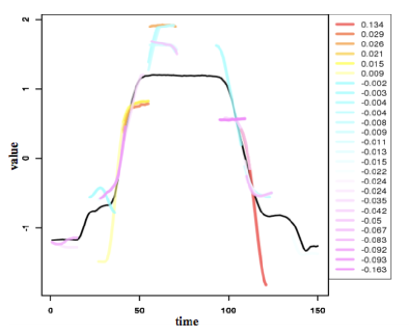
Figure 1: Visualization of discriminative pattern for an example of Gun-point data (negative label). Black line is original time series. Positive value (red to yellow line) indicates the contribution rate for positive label, and negative value (light blue to purple line) indicates the contribution rate for negative label.

Actually, for the other datasets, percentages of non-zero elements are from $0.08\%$ to $6\%$. It is clear that the solution obtained by our method has high sparsity.

Figure 1 is an example of visualization of a final hypothesis obtained by our method for Gun-point time series data. The colored lines shows all of the ${\bf x}_{k}^{(l)}$s in $g$ where both $w_{t}$ and $\alpha_{t,kl}$ are non-zero. Each value of the legends show the multiplication of $w_{t}$ and $\alpha_{t,kl}$ corresponding to ${\bf x}_{k}^{(l)}$. Since it is hard to visualize the local features over the Hilbert space, we plotted each of them to match the original time series based on Euclidean distance. In contrast to visualization analyses by time-series shapelets (see, e.g., Ye and Keogh, 2009), our visualization, colored lines and plotted position, do not strictly represent the meaning of the final hypothesis because of the non-linear feature mapping. However, we can say that colored lines represent “discriminative pattern” and certainly make important contributions to classification. Thus, we believe that our solutions are useful for domain experts to interpret important patterns.

7 Conclusion

In this paper, we show generalization error bounds of the hypothesis classes based on local features. Further, we formulate an optimization problem, which fits in the boosting framework. We design an efficient algorithm for the weak learner using DC programming techniques. Experimental results show that our method achieved competitive accuracy with the existing methods with small parameter-tuning costs.

8 Supplemental material

8.1 Proof of Lemma 3

Proof  Since $U$ can be partitioned into $\cup_{\theta\in\Theta}\{{\bf u}\in U\mid\theta_{\bf u}=\theta\}$,

$$\mathfrak{G}_{S}(H_{U}) =\frac{1}{m}\mathop{\rm E}\limits_{\boldsymbol{\sigma}}\left[\sup_{\theta\in\Theta}\sup_{{\bf u}\in U:\theta_{{\bf u}}=\theta}\sum_{i=1}^{m}\sigma_{i}\left\langle{\bf u},\Phi\left({\bf x}_{i}^{(\theta(i))}\right)\right\rangle\right]$$

$$=\frac{1}{m}\mathop{\rm E}\limits_{\boldsymbol{\sigma}}\left[\sup_{\theta\in\Theta}\sup_{{\bf u}\in U:\theta_{{\bf u}}=\theta}\left\langle{\bf u},\left(\sum_{i=1}^{m}\sigma_{i}\Phi\left({\bf x}_{i}^{(\theta(i))}\right)\right)\right\rangle\right]$$

$$\leq\frac{1}{m}\mathop{\rm E}\limits_{\boldsymbol{\sigma}}\left[\sup_{\theta\in\Theta}\sup_{{\bf u}\in U}\left\langle{\bf u},\left(\sum_{i=1}^{m}\sigma_{i}\Phi\left({\bf x}_{i}^{(\theta(i))}\right)\right)\right\rangle\right]\leq\frac{\Lambda}{m}\mathop{\rm E}\limits_{\boldsymbol{\sigma}}\left[\sup_{\theta\in\Theta}\left\|\sum_{i=1}^{m}\sigma_{i}{\bf x}_{i}^{(\theta(i))}\right\|_{\mathbb{H}}\right]$$

$$=\frac{\Lambda}{m}\mathop{\rm E}\limits_{\boldsymbol{\sigma}}\left[\sup_{\theta\in\Theta}\sqrt{\left\|\sum_{i=1}^{m}\sigma_{i}\Phi\left({\bf x}_{i}^{(\theta(i))}\right)\right\|_{\mathbb{H}}^{2}}\right]=\frac{\Lambda}{m}\mathop{\rm E}\limits_{\boldsymbol{\sigma}}\left[\sqrt{\sup_{\theta\in\Theta}\left\|\sum_{i=1}^{m}\sigma_{i}\Phi\left({\bf x}_{i}^{(\theta(i))}\right)\right\|_{\mathbb{H}}^{2}}\right]$$

$$\leq\frac{\Lambda}{m}\sqrt{\mathop{\rm E}\limits_{\boldsymbol{\sigma}}\left[\sup_{\theta\in\Theta}\left\|\sum_{i=1}^{m}\sigma_{i}\Phi\left({\bf x}_{i}^{(\theta(i))}\right)\right\|_{\mathbb{H}}^{2}\right]}.$$ (8)

The first inequality is derived from the relaxation of ${\bf u}$, the second inequality is due to Cauchy-Schwarz inequality and the fact $\|{\bf u}\|_{\mathbb{H}}\leq\Lambda$, and the last inequality is due to Jensen’s inequality. We denote by $\boldsymbol{\mathrm{K}}^{(\theta)}$ the kernel matrix such that $\boldsymbol{\mathrm{K}}_{ij}^{(\theta)}=\langle\Phi({\bf x}_{i}^{(\theta(i))}),\Phi({\bf x}_{j}^{(\theta(j))})\rangle$. Then, we have

$$\mathop{\rm E}\limits_{\boldsymbol{\sigma}}\left[\sup_{\theta\in\Theta}\left\|\sum_{i=1}^{m}\sigma_{i}\Phi\left({\bf x}_{i}^{(\theta(i))}\right)\right\|_{\mathbb{H}}^{2}\right]=\mathop{\rm E}\limits_{\boldsymbol{\sigma}}\left[\sup_{\theta\in\Theta}\sum_{i,j=1}^{m}\sigma_{i}\sigma_{j}\boldsymbol{\mathrm{K}}_{ij}^{(\theta)}\right].$$ (9)

We now derive an upper bound of the r.h.s. as follows.

For any $c>0$,

$$\exp\left(c\mathop{\rm E}\limits_{\boldsymbol{\sigma}}\left[\sup_{\theta\in\Theta}\sum_{i,j=1}^{m}\sigma_{i}\sigma_{j}\boldsymbol{\mathrm{K}}_{ij}^{(\theta)}\right]\right)\leq\mathop{\rm E}\limits_{\boldsymbol{\sigma}}\left[\exp\left(c\sup_{\theta\in\Theta}\sum_{i,j=1}^{m}\sigma_{i}\sigma_{j}\boldsymbol{\mathrm{K}}_{ij}^{(\theta)}\right)\right]$$

$$= \mathop{\rm E}\limits_{\boldsymbol{\sigma}}\left[\sup_{\theta\in\Theta}\exp\left(c\sum_{i,j=1}^{m}\sigma_{i}\sigma_{j}\boldsymbol{\mathrm{K}}_{ij}^{(\theta)}\right)\right]\leq\sum_{\theta\in\Theta}\mathop{\rm E}\limits_{\boldsymbol{\sigma}}\left[\exp\left(c\sum_{i,j=1}^{m}\sigma_{i}\sigma_{j}\boldsymbol{\mathrm{K}}_{ij}^{(\theta)}\right)\right]$$

The first inequality is due to Jensen’s inequality, and the second inequality is due to the fact that the supremum is bounded by the sum. By using the symmetry property of $\boldsymbol{\mathrm{K}}^{(\theta)}$, we have $\sum_{i,j=1}^{m}\sigma_{i}\sigma_{j}\boldsymbol{\mathrm{K}}_{ij}^{(\theta)}=\boldsymbol{\sigma}^{\top}\boldsymbol{\mathrm{K}}^{(\theta)}\boldsymbol{\sigma}$, which is rewritten as

$$\boldsymbol{\sigma}^{\top}\boldsymbol{\mathrm{K}}^{(\theta)}\boldsymbol{\sigma}=(\boldsymbol{\mathrm{V}}^{\top}\boldsymbol{\sigma})^{\top}\left(\begin{array}[]{ccc}\lambda_{1}&\hfill\hfil&0\\ \hfill\hfil&\ddots&\hfill\hfil\\ 0&\hfill\hfil&\lambda_{m}\\ \end{array}\right)\boldsymbol{\mathrm{V}}^{\top}\boldsymbol{\sigma},$$

where $\lambda_{1}\geq\dots\geq\lambda_{m}\geq 0$ are the eigenvalues of $\boldsymbol{\mathrm{K}}^{(\theta)}$ and $\boldsymbol{\mathrm{V}}=({\bf v}_{1},\ldots,{\bf v}_{m})$ is the orthonormal matrix such that ${\bf v}_{i}$ is the eigenvector that corresponds to the eigenvalue $\lambda_{i}$. By the reproductive property of Gaussian distribution, $\boldsymbol{\mathrm{V}}^{\top}\boldsymbol{\sigma}$ obeys the same Gaussian distribution as well. So,

$$\sum_{\theta\in\Theta}\mathop{\rm E}\limits_{\boldsymbol{\sigma}}\left[\exp\left(c\sum_{i,j=1}^{m}\sigma_{i}\sigma_{j}\boldsymbol{\mathrm{K}}_{ij}^{(\theta)}\right)\right]=\sum_{\theta\in\Theta}\mathop{\rm E}\limits_{\boldsymbol{\sigma}}\left[\exp\left(c\boldsymbol{\sigma}^{\top}\boldsymbol{\mathrm{K}}^{(\theta)}\boldsymbol{\sigma}\right)\right]$$

$$= \sum_{\theta\in\Theta}\mathop{\rm E}\limits_{\boldsymbol{\sigma}}\left[\exp\left(c\sum_{k=1}^{m}\lambda_{k}({\bf v}_{k}^{\top}\boldsymbol{\sigma})^{2}\right)\right]=\sum_{\theta\in\Theta}\Pi_{k=1}^{m}\mathop{\rm E}\limits_{\sigma_{k}}\left[\exp\left(c\lambda_{k}\sigma_{k}^{2}\right)\right]~{}~{}(\text{replace}~{}\boldsymbol{\sigma}={\bf v}_{k}^{\top}\boldsymbol{\sigma})$$

$$= \sum_{\theta\in\Theta}\Pi_{k=1}^{m}\left(\int_{-\infty}^{\infty}\exp\left(c\lambda_{k}\sigma^{2}\right)\frac{\exp(-\sigma)^{2}}{\sqrt{2\pi}}d\sigma\right)=\sum_{\theta\in\Theta}\Pi_{k=1}^{m}\left(\int_{-\infty}^{\infty}\frac{\exp(-(1-c\lambda_{k})\sigma^{2})}{\sqrt{2\pi}}d\sigma\right).$$

Now we replace $\sigma$ by $\sigma^{\prime}=\sqrt{1-c\lambda_{k}}\sigma$. Since $d\sigma^{\prime}=\sqrt{1-c\lambda_{k}}d\sigma$, we have:

$$\int_{-\infty}^{\infty}\frac{\exp(-(1-c\lambda_{k})\sigma^{2})}{\sqrt{2}\pi}d\sigma=\frac{1}{\sqrt{2\pi}}\int_{-\infty}^{\infty}\frac{\exp(-\sigma^{\prime 2})}{\sqrt{1-c\lambda_{k}}}d\sigma^{\prime}=\frac{1}{\sqrt{1-c\lambda_{k}}}.$$

Now, by letting $c=\frac{1}{2\max_{i,\theta}\lambda_{i}}=1/(2\lambda_{1})$ and applying the inequality that $\frac{1}{(1-x)}\leq 1+2(\sqrt{2}-1)x$ for $0\leq x\leq\frac{1}{2}$, the bound becomes

$$\exp\left(c\mathop{\rm E}\limits_{\boldsymbol{\sigma}}\left[\sup_{\theta\in\Theta}\sum_{i,j=1}^{m}\sigma_{i}\sigma_{j}\boldsymbol{\mathrm{K}}_{ij}^{(\theta)}\right]\right)\leq\sum_{\theta\in\Theta}\Pi_{k=1}^{m}\left(1+2(\sqrt{2}-1)c\lambda_{k}\right)$$ (10)

because it holds that $\frac{1}{(1-x)}\leq 1+2(\sqrt{2}-1)x$ in $0\leq x\leq\frac{1}{2}$. Further, taking logarithm, dividing the both sides by $c$ and applying $\ln(1+x)\leq x$, we get:

$$\mathop{\rm E}\limits_{\boldsymbol{\sigma}}\left[\sup_{\theta\in\Theta}\sum_{i,j=1}^{m}\sigma_{i}\sigma_{j}\boldsymbol{\mathrm{K}}_{ij}^{(\theta)}\right] \leq(\sqrt{2}-1)\sum_{k=1}^{m}\lambda_{k}+2\lambda_{1}\ln|\Theta|$$ (11)

$$=(\sqrt{2}-1)\mathrm{tr}(\boldsymbol{\mathrm{K}})+2\lambda_{1}\ln|\Theta|$$ (12)

$$\leq(\sqrt{2}-1)mR^{2}+2mR^{2}\ln|\Theta|,$$ (13)

where the last inequality holds since $\lambda_{1}=\|\boldsymbol{\mathrm{K}}\|_{2}\leq m\|\boldsymbol{\mathrm{K}}\|_{\max}\leq R^{2}$. By equation (8.1) and (11), we have:

$$\mathfrak{G}_{S}(H)\leq\frac{\Lambda}{m}\sqrt{\mathop{\rm E}\limits_{\boldsymbol{\sigma}}\left[\sup_{\theta\in\Theta}\sum_{i,j=1}^{m}\sigma_{i}\sigma_{j}\boldsymbol{\mathrm{K}}_{ij}^{(\theta)}\right]}\leq\frac{\Lambda R\sqrt{(\sqrt{2}-1)+2\ln|\Theta|}}{\sqrt{m}}.$$ (14)

 

8.2 Proof of Lemma 4

Proof  We will reduce the problem of counting intersections of the Voronoi diagrams to that of counting possible labelings by hyperplanes for some set. Note that for each neighboring Voronoi regions, the border is a part of hyperplane since the closeness is defined in terms of the inner product. So, by simply extending each border to a hyperplane, we obtain intersections of halfspaces defined by the extended hyperplanes. Note that, the size of these intersections gives an upper bound of intersections of the Voronoi diagrams. More precisely, we draw hyperplanes for each pair of points in $\mathcal{P}_{S}=\{\Phi({\bf x}_{i}^{(j)})\ \mid i\in[m],j\in[Q]\}$ so that each point on the hyperplane has the same inner product between two points. Note that for each pair ${\bf z},{\bf z}^{\prime}\in\mathcal{P}_{S}$, the normal vector of the hyperplane is given as ${\bf z}-{\bf z}^{\prime}$ (by fixing the sign arbitrary). So, the set of hyperplanes obtained by this procedure is exactly $\Phi_{\mathrm{diff}}(\mathcal{P}_{S})$. The size of $\Phi_{\mathrm{diff}}(\mathcal{P}_{S})$ is ${mQ}\choose 2$, which is at most $m^{2}Q^{2}$. Now, we consider a “dual” space by viewing each hyperplane as a point and each point in $U$ as a hyperplane. Note that points ${\bf u}$ (hyperplanes in the dual) in an intersection give the same labeling on the points in the dual domain. Therefore, the number of intersections in the original domain is the same as the number of the possible labelings on $\Phi_{\mathrm{diff}}(\mathcal{P}_{S})$ by hyperplanes in $U$. By the classical Sauer’s Lemma and the VC dimension of hyperplanes (see, e.g., Theorem 5.5 in Schölkopf and Smola (2002)), the size is at most $O((m^{2}Q^{2})^{d_{\Phi,S}^{*}})$.  

8.3 Proof of Theorem 2

Proof  (i) In this case, the Hilbert space $\mathbb{H}$is contained in $\mathbb{R}^{\ell}$. Then, by the fact that VC dimension $d_{\Phi,S}^{*}$ is at most $\ell$ and Lemma 4, the statement holds.

(ii) f $\left\langle\Phi({\bf z}),\Phi{\bf x}\right\rangle$ is monotone decreasing for $\|{\bf z}-{\bf x}\|$, then the following holds:

$$\arg\max_{{\bf x}\in\mathcal{X}}\left\langle\Phi({\bf z}),\Phi({\bf x})\right\rangle=\arg\min_{{\bf x}\in\mathcal{X}}\|{\bf z}-{\bf x}\|_{2}.$$

Therefore, $\max_{{\bf u}:\|{\bf u}\|_{\mathbb{H}}=1}\langle{\bf u},\Phi({\bf x})\rangle=\|\Phi({\bf x})\|_{\mathbb{H}}$, where ${\bf u}=\frac{\Phi({\bf x})}{\|\Phi({\bf x})\|_{\mathbb{H}}}$. It indicates that the number of Voronoi cells made by $V_{i}^{(j)}=\{{\bf z}\in\mathbb{R}^{\ell}\mid j=\arg\max_{k\in[Q]}{\bf z}\cdot{\bf x}_{i}^{(k)}\}$ corresponds to the $\hat{V}_{i}^{(j)}=\{\Phi({\bf z})\in\mathbb{H}\mid j=\arg\max_{k\in[Q]}\langle\Phi({\bf z}),\Phi({\bf x}_{i}^{(k)})\rangle\}$. Then, by following the same argument for the linear kernel case, we get the same statement.

(iii) We follow the argument in Lemma 4. For the set of classifiers $F=\{f:\Phi_{\mathrm{diff}}(\mathcal{P}_{S})\to\{-1,1\}\mid f=\mathrm{sign}(\langle{\bf u},{\bf z}\rangle),\|{\bf u}|_{\mathbb{H}},\min_{{\bf z}in\Phi_{\mathrm{diff}}(\mathcal{P}_{S})}|\langle{\bf u},{\bf z}\rangle|=\mu\}$, its VC dimension is known to be at most $R\Lambda/\mu$ for $\Phi_{\mathrm{diff}}(\mathcal{P}_{S})\subseteq\{{\bf z}\mid\|{\bf z}\|_{\mathbb{H}}\leq R\}$ (see, e.g., Schölkopf and Smola (2002)). By the definition of $\mu^{*}$, for each intersections given by hyperplanes, there always exists a point ${\bf u}$ whose inner product between each hyperplane is at least $\mu^{*}$. Therefore, the size of the intersections is bounded by the number of possible labelings in the dual space by $U^{\prime\prime}=\{{\bf u}\in\mathbb{H},\|{\bf u}\|_{\mathbb{H}}\leq\Lambda,\min_{{\bf z}in\Phi_{\mathrm{diff}}(\mathcal{P}_{S})}|\langle{\bf u},{\bf z}\rangle|=\mu^{*}\}\}$. Thus we obtain that $d_{\Phi,S}^{*}$ is at most $R\Lambda/\mu^{*}$ and by Lemma 4, we complete the proof.  

8.4 Proof of Theorem 3

Proof  We can rewrite the optimization problem (4) by using $\theta\in\Theta$ defined in Subsection 3.2 as follows:

$$\max_{\theta\in\Theta}\max_{{\bf u}\in\mathbb{H}:\theta_{\bf u}=\theta}\quad \sum_{i=1}^{m}y_{i}d_{i}\left\langle{\bf u},\Phi\left({\bf x}_{i}^{(\theta(i))}\right)\right\rangle$$ (15)

sub.to $$\|{\bf u}\|_{\mathbb{H}}^{2}\leq\Lambda^{2}.$$

Thus, if we fix $\theta\in\Theta$, we have a sub-problem. Since the constraint $\theta=\theta_{\bf u}$ can be written as linear constraints, each sub-problem is equivalent to a convex optimization. Indeed, each sub-problem can be written as the equivalent unconstrained minimization (by neglecting constants in the objective)

$$\min_{{\bf u}\in\mathbb{H}}\beta\|{\bf u}\|^{2}_{\mathbb{H}}-\sum_{i=1}^{m}\sum_{j=1}^{Q}\lambda_{i,j}\left\langle{\bf u},\Phi\left({\bf x}_{i}^{(\theta(i))}\right)\right\rangle-\sum_{i=1}^{m}y_{i}d_{i}\left\langle{\bf u},\Phi\left({\bf x}_{i}^{(\theta(i))}\right)\right\rangle,$$

where $\beta$ and $\lambda_{i,j}$ $(i\in[m],j\in[Q])$ are the corresponding positive constants. Now for each sub-problem, we can apply the standard Representer Theorem argument (see, e.g., Mohri et al. (2012)). Let $\mathbb{H}_{1}$ be the subspace $\{{\bf u}\in\mathbb{H}\mid{\bf u}=\sum_{i=1}^{m}\sum_{j=1}^{Q}\alpha_{ij}\Phi(x_{i}^{(j)}),\alpha_{ij}\in\mathbb{R}\}$. We denote ${\bf u}_{1}$ as the orthogonal projection of ${\bf u}$ onto $\mathbb{H}_{1}$ and any ${\bf u}\in\mathbb{H}$ has the decomposition ${\bf u}={\bf u}_{1}+{\bf u}^{\perp}$. Since ${\bf u}^{\perp}$ is orthogonal w.r.t. $\mathbb{H}_{1}$, $\|{\bf u}\|_{\mathbb{H}}^{2}=\|{\bf u}_{1}\|_{\mathbb{H}}^{2}+\|{\bf u}^{\perp}\|_{\mathbb{H}}^{2}\geq\|{\bf u}_{1}\|_{\mathbb{H}}^{2}$. On the other hand, $\left\langle{\bf u},\Phi\left({\bf x}_{i}^{(j)}\right)\right\rangle=\left\langle{\bf u}_{1},\Phi\left({\bf x}_{i}^{(j)}\right)\right\rangle$. Therefore, the optimal solution of each sub-problem has to be contained in $\mathbb{H}_{1}$. This implies that the optimal solution, which is the maximum over all solutions of sub-problems, is contained in $\mathbb{H}_{1}$ as well.