Gate-controlled magnon-assisted switching of magnetization in ferroelectric/ferromagnetic junctions

Abstract

Interfacing a ferromagnet with a polarized ferroelectric gate generates a non-uniform, interfacial spin density coupled to the ferroelectric polarization. This coupling allows for an electric field control of the effective field acting on the magnetization. To unravel the usefulness of this interfacial magneto-electric coupling we investigate the magnetization dynamics of a ferroelectric/ferromagnetic multilayer structure using the Landau-Lifshitz-Baryakhtar equation. The results demonstrate that the interfacial magnetoelectric coupling is utilizable as a highly localized and efficient tool for manipulating magnetism by electrical means. Ways of enhancing the strength of the interfacial coupling and/or its effects are discussed.

I Introduction

Electrical control of magnetism has the potential to boost spintronic devices with a number of novel functionalities Eerenstein:2006km ; M. Weisheit:2007 ; T. Maruyama:2009 ; D. Chiba:2011 ; Jia:2015iz . To mention an example, magnetization switching can be achieved via a spin-polarized electric current due to the spin-transfer torque or the spin-orbital torque in the presence of a spin orbital interaction J. C. Slonczewski:1996 ; L. Berger:1996 ; J. A. Katine:2000 ; M. D. Stiles:2002 ; Y. Tserkovnyak:2008 ; Brataas:2012fb ; Fan:2014hb ; Brataas:2014dla ; Oh:2016ev ; Fukami:2016kq . One may also use an electric field to manipulate the magnetization dynamics Vaz:2012dp ; T. Y. Liu:2011 ; T. Nozaki:2012 ; Brovko:2014gsb ; Schueler2017 ; Matsukura:2015hya ; Y. Shiota:2016 in which case the electric field may lead to modulations in the charge carrier density or may affect the magnetic properties such as the magnetic moment, the exchange interaction and/or the magnetic anisotropy Vaz:2012dp ; Brovko:2014gsb ; Schueler2017 ; Matsukura:2015hya . Compared to driving magnetization via a spin-polarized current, an electric field governing the magnetization has a clear advantage as it allows for non-volatile device concepts with significantly reduced energy dissipation. On the other hand, an external electric field applied to an itinerant ferromagnet (FM) is shielded by charge accumulation or depletion caused by spin-dependent screening charge that extends on a length scale of only a few angstroms into the FM Zhang:1999cx . This extreme surface confinement of screening hinders its utilization to steer the magnetic dynamics of bulk or a relatively thick nanometer-sized FM Shiota:2012dh ; Wang:2012jf . Experimentally, ultra-thin metallic FM films were thus necessary to observe an electric field influence on the dynamic of an FM Vaz:2012dp ; Brovko:2014gsb ; Nan:2014ck .

In this work we show that while the spin-polarized screening charge is surface confined, in the spin channel a local non-uniform spiral spin density builds up at the interface and goes over into the initial uniform (bulk) magnetization away from the interface. Hence, this interfacial spin spiral acts as a topological defect in the initial uniform magnetization vector field. The range of the spiral defect is set by the spin diffusion length $\lambda_{\rm m}$ J. Bass:2007 which is much larger than the charge screening length.This spin-spiral constitutes a magnetoelectric effect that has a substantial influence on the traversal magnetization dynamics of FM layers with thickness over tens of nanometers footnot . The interfacial spiral spin density can be viewed as a magnonic accumulation stabilized by the interfacial, spin-dependent charge rearrangement at the contact region between the FM and the ferroelectrics (having the FE polarization $\mathrm{P}$) and by the uniform (bulk) magnetization of FM far away from the interface Jia C. L:2014 . $\mathrm{P}$ responds to an external electric field and so does the magnetic dynamics. As shown below, this magnonic-assisted magnetoelectric coupling arising when using a dielectric FE gate, allows a (ferro)electric field control of the effective driving field that governs the magnetization switching of a FM layer with a thickness on the range of the spin diffusion length $\lambda_{\rm m}$, which is clearly of an advantage for designing spin-based, non-volatile nanoelectronic devices.

In Sec. II we discuss the mathematical details of the spin-spiral magnetoelectric coupling, followed by its implementation into the equations of motion for the magnetization dynamics in Sec. III. In Sec. IV results of numerical simulations are presented and discussed showing to which extent the spin-spiral magnetoelectric coupling can allow for the electric field control of the magnetization in FE/FM composites. Ways to enhance the effects are discussed and brief conclusions are made in Sec. V.

II Interfacial magnetoelectric coupling

Theoretically, the above magnon accumulation scenario maybe viewed as follows: When a FE layer with remanent electric polarization $\mathrm{P}$ and surface charges $\sigma_{\rm FE}$ is brought in contact with an itinerant (charge-neutral) FM, bond rearrangements occur within few atomic layers in the interface vicinity prl08andothers . On the FM side, the rearranged spin polarized charge density implies a spin configuration different from the bulk one. The modifications of the magnitude of the interfacial local magnetic moments are dictated by hybridization and charge transfer and were studied thoroughly both theoretically and experimentally (e.g., Ref.[prl08andothers, ]). Here we are interested in the consequence on the long-range magnetic order extending to the asymptotic bulk magnetization. In the mean-field formulations, the induced spin density $\mathrm{s}$ is exchange coupled with the localized magnetic moments $\mathrm{S}$, which can be treated classically as an effective magnetization $\mbox{\boldmath$\mathrm{M}$}=-\frac{g\mu_{\rm B}}{a^{3}}\mbox{\boldmath$\mathrm{S}$}$ with $\mu_{\rm B}$, $g$, and $a$ being the Bohr magneton, g-factor, and lattice constant, respectively. The associated sd exchange coupling energy at the FM interface

$$\mathcal{F}_{\rm sd}=J_{\rm sd}\frac{M}{M_{\rm s}}\mbox{\boldmath$\mathrm{s}$}\cdot{\mbox{\boldmath$\mathrm{m}$}},$$ (1)

where $\mathrm{m}$ is a unit vector in the direction of $\mathrm{M}$. $M_{\rm s}$ is the intrinsic saturation magnetization. Within the Stoner mean-field theory Soulen R.J:1998 the spin polarization $\eta$ of the electron density in transition FM metals is usually less than 1, we can decompose the induced spin density $\mathrm{s}$ as, Jia C. L:2014

$$\mbox{\boldmath$\mathrm{s}$}=\mbox{\boldmath$\mathrm{s}$}_{\rm\parallel}+\mbox{\boldmath$\mathrm{s}$}_{\rm\perp}$$ (2)

where $\mbox{\boldmath$\mathrm{s}$}_{\rm\parallel}$ represents the spin density whose direction follows adiabatically the intrinsic magnetization $\mathrm{M}$ at an instantaneous time t. $\mbox{\boldmath$\mathrm{s}$}_{\rm\perp}$ describes the transverse deviation from $\mathrm{M}$. Given that the steady-state charge accumulation entails much higher energy processes than spin excitations, in the absence of a charge current across the FE/FM interface, the spin diffusion normal to the FM/FE interface (hereafter refereed to as the $z$ direction with its origin at the interface) follows the dynamic equation (see Refs.[Jia C. L:2014, ,Manchon:2012jz, ] for details)

$$\frac{\partial\mbox{\boldmath$\mathrm{s}$}_{\rm\parallel}}{\partial t}\mbox{\boldmath$\mathrm{m}$}+\mbox{\boldmath$\mathrm{s}$}_{\rm\parallel}\frac{\partial\mbox{\boldmath$\mathrm{m}$}}{\partial t}+\frac{\partial\mbox{\boldmath$\mathrm{s}$}_{\rm\perp}}{\partial t}-D_{\rm 0}\nabla^{2}_{\rm z}\mbox{\boldmath$\mathrm{s}$}_{\rm\parallel}-D_{\rm 0}\nabla^{2}_{\rm z}\mbox{\boldmath$\mathrm{s}$}_{\rm\perp}$$

$$=-\frac{\mbox{\boldmath$\mathrm{s}$}_{\rm\parallel}}{\tau_{\rm sf}}-\frac{\mbox{\boldmath$\mathrm{s}$}_{\rm\perp}}{\tau_{\rm sf}}-\frac{\mbox{\boldmath$\mathrm{s}$}_{\rm\perp}\times\mbox{\boldmath$\mathrm{m}$}}{\tau_{\rm ex}}$$ (3)

where $D_{\rm 0}$ is the diffusion constant and $\tau_{\rm ex}\approx\hbar/(2J_{\rm sd})$. $\tau_{\rm sf}$ is the spin-flip relaxation time due to scattering with impurities, electrons, and phonons; $\tau_{\rm sf}\sim 10^{-12}-10^{-14}$ s L. Piraux:1998 and $\tau_{\rm ex}/\tau_{\rm sf}\sim 10^{-2}$ in typical FM metals J. Bass:2007 . The time-derivative terms $\frac{\partial\mbox{\boldmath$\mathrm{s}$}_{\rm\parallel}}{\partial t}$, $\frac{\partial\mbox{\boldmath$\mathrm{m}$}}{\partial t}$ and $\frac{\partial\mbox{\boldmath$\mathrm{s}$}_{\rm\perp}}{\partial t}$ below THz are negligible compared with $\mbox{\boldmath$\mathrm{s}$}/\tau_{\rm sf}$ and $\mbox{\boldmath$\mathrm{s}$}/\tau_{\rm ex}$. Thus the steady state is set by Jia C. L:2014

$$D_{\rm 0}\nabla^{2}_{\rm z}\mbox{\boldmath$\mathrm{s}$}_{\rm\parallel}=\frac{\mbox{\boldmath$\mathrm{s}$}_{\rm\parallel}}{\tau_{\rm sf}}~{}~{}~{}\text{and}~{}~{}~{}D_{\rm 0}\nabla^{2}_{\rm z}\mbox{\boldmath$\mathrm{s}$}_{\rm\perp}=\frac{\mbox{\boldmath$\mathrm{s}$}_{\rm\perp}\times\mbox{\boldmath$\mathrm{m}$}}{\tau_{\rm ex}},$$ (4)

implying an exponentially decaying spiral spin density, Jia C. L:2014

$$s_{\rm\parallel}=\eta\frac{\sigma_{\rm FM}}{\lambda_{\rm m}e}e^{-z/\lambda_{\rm m}},$$ (5)

$$\mbox{\boldmath$\mathrm{s}$}_{\rm\perp}=(1-\eta)Q_{\rm m}\frac{\sigma_{\rm FM}}{e}e^{-(1-i)\mbox{\boldmath$\mathrm{Q}$}_{\rm m}\cdot\mbox{\boldmath$\mathrm{r}$}}.$$ (6)

Here $\sigma_{\rm FM}=\sigma_{\rm FE}\approx\epsilon_{\rm FE}E$ is the surface charge density due to the electric neutrality constraint at the interface, $\epsilon_{\rm FE}$ and $E$ are the dielectric permittivity of FE and an applied normal electric field, respectively. $\lambda_{\rm m}=\sqrt{D_{\rm 0}\tau_{\rm sf}}$ is the effective spin-diffusion length and the normal spin spiral wave vector $\mbox{\boldmath$\mathrm{Q}$}_{\rm m}=\frac{1}{\sqrt{2D_{\rm 0}\tau_{\rm ex}}}\hat{\mbox{\boldmath$\mathrm{e}$}}_{\rm z}$. Clearly, in the presence of the exchange interaction with long-range FM ordering, the accumulated (magnonic) spin density extends in the FM system over a nanometer characteristic length ($\sim\lambda_{\rm m}$ being 38 $\pm$ 12 nm in Co J. Bass:2007 ) which is much larger than the electrostatic screening length (a few angstroms), albeit both are associated by largely different energy scales.

As we are interested in the effect of the low-energy accumulated magnonic density on the spin dynamic in FM we can safely assume that the spin-dependent charge excitations are frozen (because of the higher energy scale) during the (GHz-THz) spin dynamics in the FM. Treating the magnetic dynamics we consider the additional effective magnetoelectric field $\mbox{\boldmath$\mathrm{H}$}^{\rm{me}}$ acting on the magnetization dynamics $\mbox{\boldmath$\mathrm{M}$}(t)$ due to the interfacial spin order. To leading terms, from the sd interaction energy [Eq. (1)] we derive

$$\mbox{\boldmath$\mathrm{H}$}^{\rm{me}}=-\delta\mathcal{F}_{\rm sd}/\delta{\mbox{\boldmath$\mathrm{M}$}}=-\frac{J_{\rm\text{sd}}}{M_{\rm s}}\mbox{\boldmath$\mathrm{s}$}.$$ (7)

We choose nanometer thick layers Co and BaTiO₃ as prototypical FM and FE layers for estimating the characteristics of $\mbox{\boldmath$\mathrm{H}$}^{\rm me}$. The density of surface charges J. Hlinka:2006 reads $\sigma_{\rm\text{FE}}=0.27$ C/$m^{2}$ and the parameters of Co are J. M. D. Coey:2010 : $M_{\rm s}=1.44\times 10^{6}$ A/m, $K_{\rm 1}=4.1\times 10^{5}$ J/$m^{3}$, $\lambda_{\rm m}=40$ nm J. Bass:2007 , and $\eta=0.45$ Soulen R.J:1998 . We find thus $|\mbox{\boldmath$\mathrm{H}$}^{\rm{me}}|\approx 0.2$ T with $J_{\rm sd}\approx 0.1$ eV/atom and the FM thickness $d_{\rm FM}=40$ nm. Such a strong magnetoelectric field is comparable with the uniaxial anisotropic field $\frac{K_{\rm 1}}{M_{\rm s}}\approx 0.3$ T of Co. More importantly, note that the non-adiabatical component $\mbox{\boldmath$\mathrm{H}$}^{\rm{me}}_{\rm\perp}$ is always perpendicular to the direction of magnetization $\mathrm{M}$, acting as a field-like torque and a damping-like torque at all time (c.f. Fig.1), which would play a key role for electric-field assisted magnetization switching.

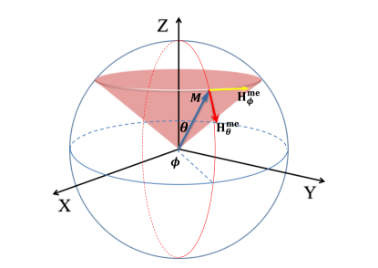
Figure 1: Schematics of the plane of variation for the magnetization $\mbox{\boldmath$\mathrm{M}$}=M\{\cos\phi\sin\theta,\sin\phi\sin\theta,\cos\theta\}$. The FM/FE interface is referred to as the $xy$ plane. $\mbox{\boldmath$\mathrm{H}$}^{\rm{me}}_{\rm\theta}$ and $\mbox{\boldmath$\mathrm{H}$}^{\rm{me}}_{\rm\phi}$ are the transversal components of the interface magnetoelectric field.

III Magnetization dynamics

We start from the Landau-Lifshitz-Baryakhtar equation (LLBar) V.G.Baryakhtar:1984 ; M.Dvornik:2013 ; Weiwei Wang:2015 for the magnetization dynamics at the FM interface,

$$\frac{\partial\mbox{\boldmath$\mathrm{M}$}}{\partial t}=-\gamma\mbox{\boldmath$\mathrm{M}$}\times\mbox{\boldmath$\mathrm{H}$}_{\rm\text{eff}}+\hat{\Lambda}_{\rm r}\cdot\mbox{\boldmath$\mathrm{H}$}_{\rm\text{eff}}-\hat{\Lambda}_{\rm e,ij}\frac{\partial^{2}\mbox{\boldmath$\mathrm{H}$}_{\rm\text{eff}}}{\partial x_{\rm i}\partial x_{\rm j}}$$ (8)

where $\gamma$ is the gyromagnetic ratio. The last two terms describe the local and nonlocal relaxations. $\hat{\Lambda}_{\rm r}$ and $\hat{\Lambda}_{\rm e}$ are generally the relaxation tensors of relativistic and exchange natures, respectively. The anisotropy of relaxations decreases with increasing temperature. Experimentally isotropy of relaxations were discussed in Ref.[Seib:2009es, ]. We can represent the relaxation tensors as $\hat{\Lambda}_{\rm r}=\lambda_{\rm r}$ and $\hat{\Lambda}_{\rm e}=\lambda_{\rm e}$ where $\lambda_{\rm r}=\gamma\alpha M_{\rm s}$ and $\lambda_{\rm e}={\gamma g\mu_{\rm B}\hbar G_{\rm 0}}/({8e^{2}})$ with $\alpha$ and $G_{\rm 0}$ being the Gilbert damping coefficient and the conductivity of FM system, respectively. $e$ is the electron charge. In contrast to the Landau-Lifshitz-Gilbert equation, the LLBar equation does not conserve the magnitude of the magnetization capturing the magnetic relaxations in metals, especially the case for FM metal interfaces. This is necessary in our case to ensure that the local magnetic order which is in equilibrium with the interface region relaxes to the asymptotic bulk magnetization.

By introducing $\mbox{\boldmath$\mathrm{M}$}=M{\mbox{\boldmath$\mathrm{m}$}}$ into the LLBar equation, we infer the following equation for the direction of magnetization Weiwei Wang:2015 ,

$$\frac{\partial\mbox{\boldmath$\mathrm{m}$}}{\partial t}=-\gamma\mbox{\boldmath$\mathrm{m}$}\times\mbox{\boldmath$\mathrm{H}$}_{\rm eff}+\frac{1}{M_{\rm s}}\mbox{\boldmath$\mathrm{R}$}_{\rm\perp}$$ (9)

with $\mbox{\boldmath$\mathrm{R}$}=\lambda_{\rm r}\mbox{\boldmath$\mathrm{H}$}_{\rm eff}-\lambda_{\rm e}\nabla^{2}_{\rm z}\mbox{\boldmath$\mathrm{H}$}_{\rm eff}$ and $\mbox{\boldmath$\mathrm{R}$}_{\rm\perp}=-\mbox{\boldmath$\mathrm{m}$}\times(\mbox{\boldmath$\mathrm{m}$}\times\mbox{\boldmath$\mathrm{R}$}).$ Here

$$\mbox{\boldmath$\mathrm{H}$}_{\rm eff}=\mbox{\boldmath$\mathrm{H}$}_{\rm eff}^{0}+\mbox{\boldmath$\mathrm{H}$}^{\rm me}$$ (10)

is the effective magnetic field, in which $\mbox{\boldmath$\mathrm{H}$}_{\rm eff}^{0}$ follows from the functional derivative of the free energy density via Sukhov:2014

$$\mbox{\boldmath$\mathrm{H}$}_{\rm eff}^{0} = -\delta\mathcal{F}_{\rm 0}/\delta\mbox{\boldmath$\mathrm{M}$},$$

$$\mathcal{F}_{\rm 0} = -K_{\rm 1}(\sin^{2}\theta\cos^{2}\phi\sin^{2}\theta_{\rm u}+\cos^{2}\theta\cos^{2}\theta_{\rm u})$$ (11)

$$-\frac{K_{\rm 1}}{2}\sin 2\theta\sin 2\theta_{\rm u}\cos\phi-(K_{\rm s}/{d_{\rm FM}}-\mu_{\rm 0}M^{2}_{\rm s}/2)\cos^{2}\theta$$

$$-\mbox{\boldmath$\mathrm{M}$}\cdot\mbox{\boldmath$\mathrm{B}$}.$$

$K_{\rm 1}$ is the uniaxial magnetocrystalline anisotropy energy, $K_{\rm s}$ is the magnetic surface anisotropy contribution which is significant for relatively thin magnetic film and favors magnetization out of the $xy$ plane. $\mu_{\rm 0}M^{2}_{\rm s}$ denotes the demagnetizing field contribution, which favors a magnetization in plane. $\mbox{\boldmath$\mathrm{M}$}\cdot\mbox{\boldmath$\mathrm{B}$}$ is the Zeemann interaction and $\theta_{\rm u}$ is the tilted angle of the easy axis from the $z$ direction.

Clearly, the non-uniform effective field $\mbox{\boldmath$\mathrm{H}$}^{\rm me}$ due to the s-d interaction with the exponentially decaying spiral spins would give rise to nonlocal damping of the magnetization dynamics. Considering that the contribution of the induced spin density to the spatial distribution of local ferromagnetic moments is small, we have

$$\langle\nabla^{2}_{\rm z}\mbox{\boldmath$\mathrm{s}$}_{\rm\perp}\rangle=2Q^{2}_{\rm m}\left(\langle s^{\phi}_{\rm\perp}\rangle\hat{\mbox{\boldmath$\mathrm{e}$}}_{\rm\theta}-\langle s^{\theta}_{\rm\perp}\rangle\hat{\mbox{\boldmath$\mathrm{e}$}}_{\rm\phi}\right).$$ (12)

Without loss of generality one can take $\langle s^{\phi}_{\rm\perp}\rangle=\langle s^{\theta}_{\rm\perp}\rangle=\frac{1}{\sqrt{2}}\langle s_{\rm\perp}\rangle$. It is also convenient to redefine some dimensionless parameters which are $\tilde{d}_{\rm FM}=\frac{d_{\rm FM}}{\lambda_{\rm m}}$, $\tilde{t}$= t$\gamma$T$\approx$ 28t GHz, and $\tilde{J}_{\rm sd}=\frac{J_{\rm sd}}{\rm eV}\frac{\sigma_{\rm FM}}{P_{\rm s}}\frac{\lambda_{\rm m}}{d_{\rm FM}}$ with the FE spontaneous polarization $P_{\rm s}$. In the following $\tilde{J}_{\rm sd}$ is taken as an adjustable parameter in view of ferroelectric tuning of magnetoelectric field $\mbox{\boldmath$\mathrm{H}$}^{\rm me}$.

IV Numerical results and discussions

For the surface anisotropy $K_{\rm s}\approx 10^{-3}$ J/$m^{2}$ and $\mu_{\rm 0}M^{2}_{\rm s}/2\approx$ 1.3$\times 10^{6}$ J/$m^{3}$ of Co sample J. M. D. Coey:2010 , the dominant contribution of the anisotropic term $(K_{\rm s}/{d_{\rm FM}}-\mu_{\rm 0}M^{2}_{\rm s}/2)$ in Eq.(11) has the form either $K_{\rm s}/{d_{\rm FM}}$, or $-\mu_{\rm 0}M^{2}_{\rm s}/2$ depending on the thickness $d_{\rm FM}$, i.e., the magnetization will be either normal to the FM interface ($\theta_{\rm u}=0$) or in the interface plane ($\theta_{\rm u}=\pi/2$).

Case I: Normal FM magnetization with $\theta_{\rm u}=0$: The free energy density is

$$\mathcal{F}_{\rm 0}=-K_{\rm eff}\cos^{2}\theta-\mbox{\boldmath$\mathrm{M}$}\cdot\mbox{\boldmath$\mathrm{B}$},\quad K_{\rm eff}=K_{\rm 1}+\frac{K_{\rm s}}{d_{\rm FM}}-\frac{\mu_{\rm 0}M_{\rm s}^{2}}{2}$$ (13)

which leads to

$$\mbox{\boldmath$\mathrm{H}$}^{0}_{\rm eff}=\frac{2K_{\rm eff}}{M_{\rm s}}\cos\theta\hat{\mbox{\boldmath$\mathrm{e}$}}_{\rm z}$$ (14)

without an applied magnetic field $\mathrm{B}$. The LLBar equation reads then,

$$\frac{\partial\theta}{\partial\tilde{t}}=\frac{\gamma^{e}_{\rm+}}{\sqrt{2}}{H}^{\rm me}_{\rm\perp}-\alpha\frac{K_{\rm eff}}{M_{\rm s}}\sin 2\theta,$$ (15)

$$\sin\theta\frac{\partial\phi}{\partial\tilde{t}}=-\frac{\gamma^{e}_{\rm-}}{\sqrt{2}}{H}^{\rm me}_{\rm\perp}+\frac{K_{\rm eff}}{M_{\rm s}}\sin 2\theta$$ (16)

with $\gamma^{e}_{\rm\pm}=1-2Q^{2}_{\rm m}\frac{\lambda_{\rm e}}{\gamma M_{\rm s}}\pm\frac{\lambda_{\rm r}}{\gamma M_{\rm s}}=\gamma^{e}\pm\alpha$ .

Clearly, under a weak interfacial ME field, the condition

$${H}^{\rm me}_{\rm\perp}=\sqrt{2}\frac{\alpha}{\gamma^{e}_{\rm+}}\frac{K_{\rm eff}}{M_{\rm s}}\sin 2\theta$$ (17)

can be satisfied, the polar angle $\theta$ ends up processionally in the equilibrium state [c.f. Fig.2(a) with ${\partial\theta}/{\partial\tilde{t}}=0$]. Otherwise, the strong transversal field ${H}^{\rm me}_{\rm\perp}$ results in a magnetization flip over the normal $\hat{\mbox{\boldmath$\mathrm{e}$}}_{\rm z}$-direction [Fig.2(b)]. Considering that the ME field depends linearly on the applied electric field and the reciprocal of FM thickness, one would expect a transition from the magnetization procession around the z axis (for a small electric field $E$ and/or relatively thick FM layers) to the magnetization flip over the normal direction (for a strong electric field and/or ultra-thin FM film) at the critical points, as demonstrated in Figs. 2(c) and 2(d).

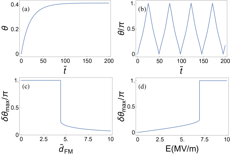
Figure 2: Dynamics of the normal magnetization. The polar angle $\theta$ vs. dimensionless time $\tilde{t}$ for different ME field (a) $\tilde{J}_{\rm sd}=0.005$ and (b) $\tilde{J}_{\rm sd}=0.03$, respectively. Panels (c) and (d) demonstrate the thickness and electric-field dependence of $\delta\theta_{\rm max}=\theta_{\rm max}-\theta(0)$, where $\theta(0)$ and $\theta_{\rm max}$ are respectively the initial value ($\theta(0)=0$) and the maximum value of the polar angle during the time evolution of magnetization. $\delta\theta_{\rm max}=\pi$ indicates a magnetization flip over the normal $\hat{\mbox{\boldmath$\mathrm{e}$}}_{\rm z}$ direction. Here, $\alpha=0.1$, $\epsilon_{\rm FE}=1000$ and $K_{\rm eff}\sim K_{\rm 1}$.

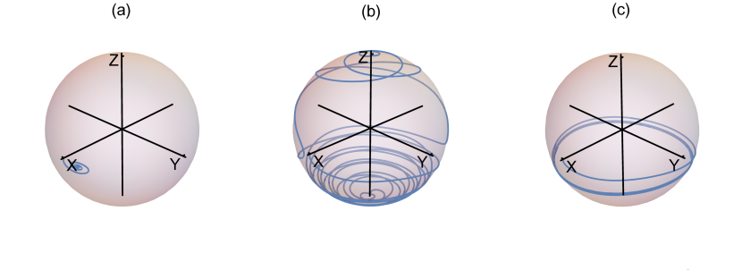
Figure 3: Dynamics of the in-plane magnetization for different interface ME field and anisotropic field: (a) ${\tilde{J}}_{\rm sd}=0.03$ and $2K_{\rm 1}/M_{\rm s}=0.6$ T, (b) ${\tilde{J}}_{\rm sd}=0.03$ and $2K_{\rm 1}/M_{\rm s}=0.3$ T, and (c) ${\tilde{J}}_{\rm sd}=0.015$ and $2K_{\rm 1}/M_{\rm s}=0.1$ T, respectively. Here ${\tilde{d}}_{\rm FM}=1$ and $\alpha=0.1$.

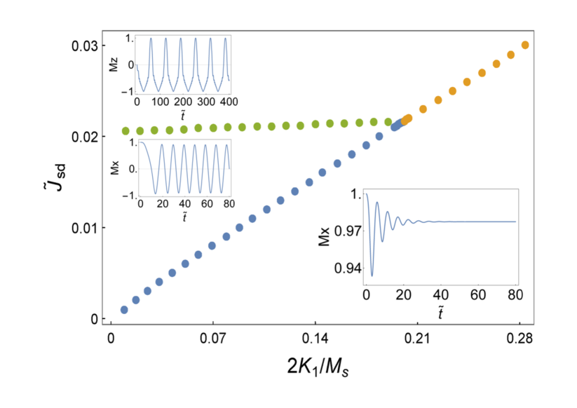
Figure 4: Phase diagrams of the in-plane magnetization dynamics with $\alpha=0.1$, $\tilde{d}_{\rm FM}=1$, and $\mbox{\boldmath$\mathrm{B}$}=0$: (a) the localized precessional mode, (b) the $z$-axial flip mode, and (c) the $z$-axial rotational mode, respectively. The characterization of dynamic behavior of magnetization in three different phases is illustrated in Fig.3. Insets show the corresponding time evolution of magnetization in each phase.

Case II: In-plane magnetization with $\theta_{\rm u}=\pi/2$: Disregarding the surface anisotropy ($K_{\rm s}/d_{\rm FM}\ll\mu_{\rm 0}M^{2}_{\rm s}/2$) for a thick FM film, the effective magnetic field reads

$$\mbox{\boldmath$\mathrm{H}$}^{0}_{\rm eff}=2K_{\rm 1}/M_{\rm s}\sin\theta\cos\phi\hat{\mbox{\boldmath$\mathrm{e}$}}_{\rm x}-\mu_{\rm 0}M_{\rm s}\cos\theta\hat{\mbox{\boldmath$\mathrm{e}$}}_{\rm z}+\mbox{\boldmath$\mathrm{B}$}$$ (18)

and the magnetization favors an in-plane $\hat{\mbox{\boldmath$\mathrm{e}$}}_{\rm x}$ axis, which means $\phi(0)=0$ with the external magnetic field $\mbox{\boldmath$\mathrm{B}$}=0$. Upon some simplifications the LLBar equation reads

$$\frac{\partial\theta}{\partial\tilde{t}} = \frac{\gamma^{e}_{\rm+}}{\sqrt{2}}{H}^{\rm me}_{\rm\perp}+\alpha\frac{\mu_{\rm 0}M_{\rm s}}{2}\sin 2\theta+\alpha\frac{K_{\rm 1}}{M_{\rm s}}\sin 2\theta\cos^{2}\phi$$ (19)

$$- \frac{K_{\rm 1}}{M_{\rm s}}\sin\theta\sin 2\phi+\alpha B\cos\theta\cos\phi-B\sin\phi,$$

$$\sin\theta\frac{\partial\phi}{\partial\tilde{t}} = -\frac{\gamma^{e}_{\rm-}}{\sqrt{2}}{H}^{\rm me}_{\rm\perp}-\frac{\mu_{\rm 0}M_{\rm s}}{2}\sin 2\theta-\alpha\frac{K_{\rm 1}}{M_{\rm s}}\sin\theta\sin 2\phi$$ (20)

$$- \frac{K_{\rm 1}}{M_{\rm s}}\sin 2\theta\cos^{2}\phi-B\cos\theta\cos\phi-\alpha B\sin\phi.$$

In the absence of external magnetic field $\mathrm{B}$, the magnetization dynamics is determined by three parameters: $\alpha$, $H^{\rm me}_{\rm\perp}$, and $K_{\rm 1}/M_{\rm s}$. Firstly, let us ignore the damping terms for small Gilbert damping coefficient $\alpha$, the weak ME field $H^{\rm me}_{\rm\perp}$ would satisfy $\frac{\partial\theta}{\partial\tilde{t}}=0$ and $\frac{\partial\phi}{\partial\tilde{t}}=0$, resulting in a relocation of the magnetization with an equilibrium tilted angle in the vicinity of $x$ axis, as shown in Fig.3(a). However, when $H^{\rm me}_{\rm\perp}$ is stronger than the anisotropic field $K_{\rm 1}/M_{\rm s}$ and the demagnetization field $\mu_{\rm 0}M_{\rm s}$, no solutions exist for $\partial\theta/\partial\tilde{t}=0$ at all time, the magnetization possesses a $z$-axial flip mode in the whole spin space [c.f. Fig.3(b)] similar to the case of normal FM magnetization. On the other hand, after accounting for terms containing $\alpha$ in the LLBar equations, we would have additional magnetization rotation around the $z$ axis [Fig.3(c)]. Further insight into the detailed characterization of magnetization dynamics is delivered by numerics for a varying strength of the ME field $\tilde{J}_{\rm sd}$ and the uniaxial anisotropy $K_{\rm 1}/M_{\rm s}$ in Fig.4 with $\alpha=0.1$. There are two new phases, the $z$-axial flip mode and the $z$-axial rotational mode, which were unobserved in the FM systems in the absence of interface ME interaction. With decreasing the damping $\alpha$, the area of the $z$-axial rotational mode shrinks vanishing eventually. By applying an external magnetic field $\mathrm{B}$ along the $x$-direction, only slight modifications are found in the phase diagram. However, the initial azimuthal angle $\phi(0)$ deviates from the easy axis with a rotating magnetic field $\mathrm{B}$ in the $xy$ interface plane. Considering the LLBar equations with the initial condition $\theta(t=0)=\pi/2$, we have

$$\frac{\partial\theta}{\partial\tilde{t}}|_{\rm\tilde{t}=0}\approx\frac{\gamma^{e}_{\rm+}}{\sqrt{2}}\mbox{\boldmath$\mathrm{H}$}^{s-d}_{\rm\perp}-\frac{K_{\rm 1}}{M_{\rm s}}\sin 2\phi(0)$$ (21)

with a small damping $\alpha$. As the dynamic equation is sensitive to the initial azimuthal angle $\phi(0)$, the calculations show that the magnetization dynamics may change between the processional mode around the $x$ axis and the $z$-axial flip or $z$-axial rotational mode, depending on the initial value of $\phi(0)$.

Phenomenologically, such an $z$-axial flip mode and $z$-axial rotational mode are exhibited as a precessional motion of the magnetization with a negative damping, as shown in the experimental observation for polycrystalline CoZr/plumbum magnesium niobate-plumbum titanate (PMN-PT) heterostructures Jia:2015iz , where an emergence of positive-to-negative transition of magnetic permeability was observed by applying external electric field. There is also some analogy between these non-equilibrium switching behaviors in FM/FE heterostructures and the negative damping phenomenon in trilayer FM/normal metal/FM structures, in which the supplying energy is thought to be provided by injecting spin-polarized electrons from an adjacent FM layer, magnetized in the opposite direction compared to the FM layer under consideration Shufeng Zhang:2009 ; M-Book .

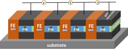
Figure 5: Schematic structure diagram of the FE/FM multilayer system with enhanced ME effects. The arrows mark the directions of the FE polarization $\mathrm{P}$ and the FM magnetization $\mathrm{M}$, respectively.

V Conclusion and outlook

The above theoretical considerations along with numerical simulations for specific material FE/FM composites endorse that the magnetization dynamics can be controlled by an electric field of a moderate strength. The excitations triggered by the electric field are transferred to the spin system via the interface spiral-mediated magnetoelectric coupling and may result in a magnetization switching. This direct electric field control of magnetization switching offers a qualitatively different way to manipulate magnetic devices swiftly with low-power write capability. On the other hand, even though the spin-mediated magnetoelectric coupling has a much longer range that the surface localized charge-mediated FE/FM coupling, its range is still limited by the spin diffusion length which is material dependent but yet in the range of several tens of nanometers. Hence, the full power of the predicted effect is expected for multilayer systems such as those schematically shown in Fig.5: Starting from a bilayer structure with a thick FE interfaced with a FM layer which has a thickness in the range of the spin diffusion length, we suggest to cap this structure with a spacer layer, for instance an (oxide) insulator. Repeating the whole structure as proposed in Fig.5 allows for a simple serial extension from a double to multilayer structure while enhancing the influence of the magnetoelectric coupling.

VI Acknowledgment

This work is supported the National Natural Science Foundation of China (Grant No. 11474138), the German Research Foundation (Grant No. SFB 762), the Program for Changjiang Scholars and Innovative Research Team in University (Grant No. IRT-16R35), and the Fundamental Research Funds for the Central Universities.

References

- (1) W. Eerenstein, N. D. Mathur, and J. F., Scott, Multiferroic and magnetoelectric materials, Nature 442,759 (2006).
- (2) M. Weisheit, S. Fähler, A. Marty, Y. Souche, C. Poinsignon, and D. Givord, Electric Field-Induced Modification of Magnetism in Thin-Film Ferromagnets, Science 315,349 (2007).
- (3) T. Maruyama et al., Large voltage-induced magnetic anisotropy change in a few atomic layers of iron, Nat. Nanotechnol. 4,158 (2009).
- (4) D. Chiba, S. Fukami, K. Shimamura, N. Ishiwata, K. Kobayashi, and T. Ono, Electrical control of the ferromagnetic phase transition in cobalt at room temperature, Nat. Mater. 10,853 (2011).
- (5) C. L. Jia, F. L. Wang, C. J. Jiang, J. Berakdar, D. S. Xue, Electric tuning of magnetization dynamics and electric field-induced negative magnetic permeability in nanoscale composite multiferroics, Sci. Rep. 5,11111 (2015).
- (6) J. C. Slonczewski, Current-driven excitation of magnetic multilayers, J. Magn. Magn. Mater. 159, L1 (1996).
- (7) L. Berger, Emission of spin waves by a magnetic multilayer traversed by a current, Phys. Rev. B 54,9353 (1996).
- (8) J. A. Katine, F. J. Albert, R. A. Buhrman, E. B. Myers, and D. C. Ralph, Current-Driven Magnetization Reversal and Spin-Wave Excitations in Co/Cu/Co Pillars, Phys. Rev. Lett. 84,3149 (2000).
- (9) A. Brataas, A. D. Kent & H. Ohno, Current-induced torques in magnetic materials, Nat. Mater. 11,372 (2012).
- (10) Y. Fan et al., Magnetization switching through giant spin-orbit torque in a magnetically doped topological insulator heterostructure, Nature Materials 13,699 (2014).
- (11) A. Brataas, K. M. D. Hals, Spin-orbit torques in action, Nature Nanotech 9, 86 (2014).
- (12) M. D. Stiles, A. Zangwill, Anatomy of spin-transfer torque, Phys. Rev. B 66, 014407 (2002).
- (13) Y.-W. Oh et.al. Field-free switching of perpendicular magnetization through spin-orbit torque in antiferromagnet/ferromagnet/oxide structures, Nature Nanotech 11, 878 (2016).
- (14) S. Fukami, T. Anekawa, C. Zhang, and H. Ohno, A spin-orbit torque switching scheme with collinear magnetic easy axis and current configuration, Nature Nanotech 11, 621 (2016).
- (15) Y. Tserkovnyak, A. Brataas, and G. E. Bauer, Theory of current-driven magnetization dynamics in inhomogeneous ferromagnets, J. Magn. Magn. Mater. 320,1282 (2008).
- (16) C. A. F. Vaz, Electric field control of magnetism in multiferroic heterostructures, J. Phys.: Condens. Mat. 24, 333201 (2012).
- (17) O. O. Brovko, P. Ruiz-Diaz, T. R. Dasa, and V.S. Stepanyuk, Controlling magnetism on metal surfaces with non-magnetic means: electric fields and surface charging, J. Phys.: Condens. Mat. 26, 093001 (2014).
- (18) M. Sch ler, L. Chotorlishvili, M. Melz, A. Saletsky, A. Klavsyuk, Z. Toklikishvili, and J. Berakdar, Functionalizing Fe adatoms on Cu(001) as a nanoelectromechanical system New J. Phys. 19, 073016 (2017).
- (19) F. Matsukura, Y. Tokura, H. Ohno, Control of magnetism by electric fields, Nat. Nanotechnol. 10,209 (2015).
- (20) T. Y. Liu and G. Vignale, Electric Control of Spin Currents and Spin-Wave Logic, Phys. Rev. Lett. 106,247203 (2011).
- (21) T. Nozaki et al., Electric-field-induced ferromagnetic resonance excitation in an ultrathin ferromagnetic metal layer, Nature Phys. 8,491 (2012).
- (22) Y. Shiota, S. Miwa, S. Tamaru, T. Nozaki et al., Field angle dependence of voltage-induced ferromagnetic resonance under DC bias voltage, J. Magn. Magn. Mater. 400,159 (2016)
- (23) S. Zhang, Spin-Dependent Surface Screening in Ferromagnets and Magnetic Tunnel Junctions, Phys. Rev. Lett. 83, 640 (1999).
- (24) Y. Shiota et al. Induction of coherent magnetization switching in a few atomic layers of FeCo using voltage pulses. Nature Materials 11, 39 (2012).
- (25) W.-G. Wang, M. Li, S. Hageman, and C.-L. Chien, Electric-field-assisted switching in magnetic tunnel junctions. Nature Materials 11, 64 (2012).
- (26) T. Nan, Z. Zhou, M. Liu, X. Yang, Y. Gao, B.A. Assaf, H. Lin, S. Velu, X. Wang, H. Luo, J. Chen, S. Akhtar, E. Hu, R. Rajiv, K. Krishnan, S. Sreedhar, D. Heiman, B.M. Howe, G.J. Brown, and N.X. Sun, Quantification of strain and charge co-mediated magnetoelectric coupling on ultra-thin Permalloy/PMN-PT interface, Sci. Rep. 4, 3688 (2014).
- (27) J. Bass and W. P. Pratt Jr., Spin-diffusion lengths in metals and alloys, and spin-flipping at metal/metal interfaces: an experimentalist’s critical review, J. Phys.: Condens. Matter 19,183201(2007).
- (28) The longitudinal FM dynamics is mostly dictated by charge screening/rearrangement right at the interface and can still be useful for device concepts, as discussed for instance in Ref.wang2017, .
- (29) X.-G.- Wang et al. Electrically driven magnetic antenna based on multiferroic composites, J. Phys.: Condens. Matter 29, 095804 (2017).
- (30) C.-L. Jia, T.-L. Wei, C.-J. Jiang, D. S.Xue, A. Sukhov, and Berakdar, Mechanism of interfacial magnetoelectric coupling in composite multiferroics, Phys. Rev. B 90, 054423 (2014).
- (31) C-G. Duan, S. S. Jaswal and E. Y. Tsymbal, predicted magnetoelectric effect in Fe/BaTiO3 multilayers: Ferroelectric control of magnetism Phys. Rev. Lett. 97, 047201 (2006); H. L. Meyerheim et al. Structural Secrets of Multiferroic Interfaces Phys. Rev. Lett. 106 087203 (2011).
- (32) R. J. Soulen Jr. et al., Measuring the Spin Polarization of a Metal with a Superconducting Point Contact, Science 282,85(1998).
- (33) A. Manchon, R. Matsumoto, H. Jaffres, and J. Grollier, Spin transfer torque with spin diffusion in magnetic tunnel junctions, Phys. Rev. B 86, 060404 (2012).
- (34) L. Piraux, S. Dubois, A. Fert, and L. Belliard, The temperature dependence of the perpendicular giant magnetoresistance in Co/Cu multilayered nanowires, Eur. Phys. J. B 4, 413-420 (1998)
- (35) J. Hlinka and P. Márton, Phenomenological model of a domain wall in BaTiO3-type ferroelectrics, Phys. Rev. B 74,104104(2006)
- (36) J. M. D. Coey, Magnetism and Magnetic Materials (Cambridge University Press, Cambridge, UK, 2010).
- (37) V. G. Baryakhtar, Phenomenological description of relaxation processes in magnetic materials, Zh. Eksp. Teor. Fiz 87, 1501 (1984) [Sov. Phys. JETP 60, 863 (1984)]
- (38) M. Dvornik, A. Vansteenkiste, and B. Van. Waeyenberge, Micromagnetic modeling of anisotropic damping in magnetic nanoelements, Phys. Rev. B 88,054427(2013).
- (39) W. Wang et al., Phenomenological description of the nonlocal magnetization relaxation in magnonics, spintronics, and domain-wall dynamics, Phys. Rev. B 92,054430(2015).
- (40) J. Seib, D. Steiauf, and M. Fähnle, M. Linewidth of ferromagnetic resonance for systems with anisotropic damping. Phys. Rev. B 79, 092418 (2009).
- (41) A. Sukhov, C. L. Jia, L. Chotorlishvili, P. P. Horley, D. Sander, and J. Berakdar, Angular dependence of ferromagnetic resonance as indicator of the nature of magnetoelectric coupling in ferromagnetic-ferroelectric heterostructures, Phys. Rev. B 90,224428 (2014).
- (42) Shufeng Zhang, Steven S and L Zhang, Generalization of the Landau-Lifshitz-Gilbert Equation for Conducting Ferromagnets, Phys. Rev. Lett. 102,086601(2009).
- (43) J. Stöhr and H.C. Sigmann, Magnetism: From Fundamentals to Nanoscale Dynamics, (Springer-Verlag, Heidelberg, 2006)