Passivity based design of sliding modes for optimal Load Frequency Control^⋆

Abstract

This paper proposes a distributed sliding mode control strategy for optimal Load Frequency Control (OLFC) in power networks, where besides frequency regulation also minimization of generation costs is achieved (economic dispatch). We study a nonlinear power network partitioned into control areas, where each area is modelled by an equivalent generator including voltage and second order turbine-governor dynamics. The turbine-governor dynamics suggest the design of a sliding manifold, such that the turbine-governor system enjoys a suitable passivity property, once the sliding manifold is attained. This work offers a new perspective on OLFC by means of sliding mode control, and in comparison with existing literature, we relax required dissipation conditions on the generation side and assumptions on the system parameters.

I Introduction

A power mismatch between generation and demand gives rise to a frequency in the power network that can deviate from its nominal value. Regulating the frequency back to its nominal value by Load Frequency Control (LFC) is challenging and it is uncertain if current implementations are adequate to deal with an increasing share of renewable energy sources [2]. Traditionally, the LFC is performed at each control area by a primary droop control and a secondary proportional-integral (PI) control. To cope with the increasing uncertainties affecting a control area and to improve the controller’s performance, advanced control techniques have been proposed to redesign the conventional LFC schemes, such as model predictive control (MPC) [3], adaptive control [4], fuzzy control [5] and sliding mode (SM) control. However, due to the predefined power flows through the tie-lines, the possibility of achieving economically optimal LFC is lost [6]. Besides improving the stability and the dynamic performance of power systems, new control strategies are additionally required to reduce the operational costs of LFC [7]. In this paper we propose a novel distributed optimal LFC (OLFC) scheme that incorporates the economic dispatch into the LFC loop, departing from the conventional tie-line requirements. An up-to-date survey on recent results on offline and online optimal power flows and OLFC can be found in [8]. We restrict ourselves here to a brief overview of online solutions to OLFC that are close to the presented work. Particularly, we focus on distributed solutions, in contrast to more centralized control schemes that have been studied in e.g. [9, 10, 11]. In order to obtain OLFC, the vast majority of distributed solutions appearing in the literature fit in one of two categories. First, the economic dispatch problem is distributively solved by a primal-dual algorithm converging to the solution of the associated Lagrangian dual problem [12, 13, 14, 15, 16, 17, 18, 19, 20, 21, 22, 23]. This approach generally requires measurements of the loads or the power flows, which is not always desirable in a LFC scheme. This issue is avoided by the second class of solutions, where a distributed consensus algorithm is employed to converge to a state of identical marginal costs, solving the economic dispatch problem in the unconstrained case [24, 25, 26, 27, 28, 29, 30, 31, 32, 33, 34, 35, 36]. The proposed sliding mode controller design in this work is compatible with both approaches, although we put the emphasize on a distributed consensus based solution and remark on the primal-dual based approach.

I-A Main contributions

Sliding mode control has been used to improve the conventional LFC schemes [37], possibly together with disturbance observers [38]. However, the proposed use of SM to obtain a distributed OLFC scheme is new and can offer a few advantages over the previous results on OLFC. Foremost, it is possible to incorporate the widely used second order model for the turbine-governor dynamics that is generally neglected in the analytical OLFC studies. Since the generated control signals in OLFC schemes adjust continuously and in real-time the governor set points, it is important to incorporate the generation side in a satisfactory level of detail. In this paper, we adopt a nonlinear model of a power network, including voltage dynamics, partitioned into control areas having an arbitrarily complex and meshed topology. The generation side is modelled by an equivalent generator including voltage dynamics and second order turbine-governor dynamics, which is standard in studies on conventional LFC schemes. We propose a distributed SM controller that is shown to achieve frequency control, while minimizing generation costs. The proposed control scheme continuously adjusts the governor set point. Conventional SM controllers can suffer from the notorious drawback known as chattering effect, due to the discontinuous control input. To alleviate this issue, we incorporate the well known Suboptimal Second Order Sliding Mode (SSOSM) control algorithm [39] leading to a continuous control input. To design the controllers obtaining OLFC, we recall an incremental passivity property of the power network [25] that prescribes a suitable sliding manifold. Particularly, the non-passive turbine-governor system, constrained to this manifold, is shown to be incrementally passive allowing for a passive feedback interconnection, once the closed-loop system evolves on the sliding manifold. The proposed approach differs substantially from two notable exceptions that also incorporate the turbine-governor dynamics ([40], [41]) and shows some benefits. In contrast to [40], we do not impose constraints on the permitted system parameters, and in contrast to [41] we do not impose dissipation assumptions on the generation side and allow for a higher relative degree (see also Remark 8). Furthermore, we believe that the chosen approach, where the design of the sliding manifold is inspired by desired passivity properties, offers new perspectives on the control of networks that have similar control objectives as the one presented, e.g. achieving power sharing in microgrids. As this paper is (to the best of our knowledge) the first to use sliding mode control to obtain OLFC, it additionally enables further studies to compare the performance with respect to other approaches found in the literature.

I-B Outline

The present paper is organized as follows. In Section II the network model is introduced. In Section III the considered OLFC problem is formulated. The proposed controller is described and analyzed in Section IV and V, respectively. Simulation results are reported and discussed in Section VI, while some conclusions are finally gathered in Section VII.

II Nonlinear power network model

Figure 1: Block diagram of two interconnected control areas. The voltage dynamics are omitted.

Consider a power network consisting of $n$ interconnected control areas. The network topology is represented by a connected and undirected graph $\mathcal{G}=(\mathcal{V},\mathcal{E})$, where the nodes $\mathcal{V}=\{1,...,n\}$, represent the control areas and the edges $\mathcal{E}=\{1,...,m\}$, represent the transmission lines connecting the areas. The topology can be described by its corresponding incidence matrix $\mathcal{B}\in\mathds{R}^{n\times m}$. Then, by arbitrarily labeling the ends of edge $k$ with a $+$ and a $-$, one has that

$$\mathcal{B}_{ik}=\begin{cases}+1\quad&\text{if $i$ is the positive end of $k$}\\ -1\quad&\text{if $i$ is the negative end of $k$}\\ ~{}~{}0\quad&\text{otherwise}.\end{cases}$$

A control area is represented by an equivalent generator and a load, where the governing dynamics of the $i$-th area are described by the so called ‘flux-decay’ or ‘single-axis model’ given as [42]:

$$\dot{\delta}_{i}= ~{}f_{i}$$

$$T_{pi}\dot{f}_{i}= -f_{i}+K_{pi}\Big{(}P_{ti}-P_{di}+\sum_{j\in\mathcal{N}_{i}}V_{i}V_{j}B_{ij}\sin{(\delta_{i}-\delta_{j})}\Big{)}$$

$$T_{Vi}\dot{V}_{i}= ~{}\overline{E}_{fi}-\big{(}1-(X_{di}-X_{di}^{\prime})B_{ii}\big{)}V_{i}$$ (1)

$$-(X_{di}-X_{di}^{\prime})\sum_{j\in\mathcal{N}_{i}}V_{j}B_{ij}\cos{(\delta_{i}-\delta_{j})},$$

where $\mathcal{N}_{i}$ is the set of control areas connected to the $i$-th area by transmission lines. Note that we assume that the network is lossless, which is generally valid in high voltage transmission networks where the line resistance is negligible. Moreover, $P_{ti}$ in (1) is the power generated by the $i$-th (equivalent) plant and can be expressed as the output of the following second order dynamical system that describes the behaviour of both the governor and the turbine:

$$\begin{split}T_{ti}\dot{P}_{ti}=&-P_{ti}+P_{gi}\\ T_{gi}\dot{P}_{gi}=&-\frac{1}{R_{i}}f_{i}-P_{gi}+u_{i}.\end{split}$$ (2)

The symbols used in (1) and (2) are described in Table I. To further illustrate the dynamics, a block diagram for a two area network is provided in Figure 1. In this paper we aim at the design of a continuous control input $u_{i}$ to achieve both frequency regulation and economic efficiency (optimal Load Frequency Control).

TABLE I: Description of the used symbols

	State variables
$\delta_{i}$	Voltage angle
$f_{i}$	Frequency deviation
$V_{i}$	Voltage
$P_{ti}$	Turbine output power
$P_{gi}$	Governor output
	Parameters
$T_{pi}$	Time constant of the control area
$T_{ti}$	Time constant of the turbine
$T_{gi}$	Time constant of the governor
$T_{Vi}$	Direct axis transient open-circuit constant
$K_{pi}$	Gain of the control area
$R_{i}$	Speed regulation coefficient
$X_{di}$	Direct synchronous reactance
$X^{\prime}_{di}$	Direct synchronous transient reactance
$B_{ij}$	Transmission line susceptance
	Inputs
$u_{i}$	Control input to the governor
$\overline{E}_{fi}$	Constant exciter voltage
$P_{di}$	Unknown power demand

To study the power network we write system (1) compactly for all areas $i\in\mathcal{V}$ as

$$\begin{split}\dot{\eta}=&~{}\mathcal{B}^{T}f\\ T_{p}\dot{f}=&-f+K_{p}(P_{t}-P_{d}{\color[rgb]{0,0,0}}\mathcal{B}\Gamma(V)\sin(\eta))\\ T_{V}\dot{V}=&-(X_{d}-X^{\prime}_{d})E(\eta)V+\overline{E}_{f},\\ \end{split}$$ (3)

and the turbine-governor dynamics in (2) as

$$\begin{split}T_{t}\dot{P}_{t}=&-P_{t}+P_{g}\hskip 108.12054pt\\ T_{g}\dot{P}_{g}=&-R^{-1}f-P_{g}+u,\end{split}$$ (4)

where $\eta=\mathcal{B}^{T}\delta\in\mathds{R}^{m}$ is vector describing the differences in voltage angles. Furthermore, $\Gamma=\operatorname{diag}\{\Gamma_{1},\dots,\Gamma_{m}\}$, where $\Gamma(V)_{k}=V_{i}V_{j}B_{ij}$, with $k\sim\{i,j\}$, i.e., line $k$ connects areas $i$ and $j$. The components of the matrix $E(\eta)\in\mathds{R}^{n\times n}$ are defined as

$$\begin{split}E_{ii}(\eta)=&\frac{1}{X_{di}-X^{{}^{\prime}}_{di}}-B_{ii}\hskip 32.00002pti\in\mathcal{V}\\ E_{ij}(\eta)=&~{}B_{ij}\cos(\eta_{k})=E_{ji}(\eta)\hskip 11.99998ptk\sim\{i,j\}\in\mathcal{E}\\ E_{ij}(\eta)=&~{}0\hskip 92.0001pt~{}\text{otherwise}.\end{split}$$ (5)

The remaining symbols follow straightforwardly from (1) and (2), and are vectors and matrices of suitable dimensions.

Remark 1

(Reactance and susceptance) For each (equivalent) generator $i\in\mathcal{V}$, the reactance is higher than the transient reactance, i.e. $X_{di}>X^{\prime}_{di}$ [43]. Furthermore, the self-susceptance of area $i\in\mathcal{V}$ is given by $B_{ii}=\sum_{j\in\mathcal{N}_{i}}B_{ij}$ and the susceptance of a line satisfies $B_{ij}=B_{ji}<0$. Consequently, $E(\eta)$ is a strictly diagonally dominant and symmetric matrix with positive elements on its diagonal and is therefore positive definite. $\hfill\diamond$

To permit the controller design in the next sections, the following assumption is made on the unknown demand (unmatched disturbance) and the available measurements:

Assumption 1

(Available information) The variables $f_{i},P_{ti}$ and $P_{gi}$ are locally available at control area $i$. The unmatched disturbance $P_{di}$ is unknown, and can be bounded as $\lvert P_{di}\rvert\leq\mathcal{D}_{i},$ where $\mathcal{D}_{i}$ is a positive constant available at control area $i$. $\hfill\diamond$

In case not all variables are locally available, Assumption 1 can be relaxed by implementing observers that estimate the unmeasured states in a finite time (see for instance [44]).

III Incremental passivity of the power network

In this section we recall a useful incremental passivity property of system (3) that has been established before in [25]. To facilitate the discussion, we first define ‘incremental passivity’.

Definition 1

(Incremental passivity) System

$$\begin{split}\dot{x}=&~{}\zeta(x,u)\\ y=&~{}h(x),\end{split}$$ (6)

$x\in\mathds{R}^{n}$, $u,y\in\mathds{R}^{m}$, is incrementally passive with respect to a constant triplet $(\overline{x},\overline{u},\overline{y})$ satisfying

$$\begin{split}\boldsymbol{0}=&~{}\zeta(\overline{x},\overline{u})\\ \overline{y}=&~{}h(\overline{x}),\end{split}$$ (7)

if there exists a continuously differentiable function $\mathcal{S}:\mathds{R}^{n}\rightarrow\mathds{R}_{+}$, such that for all $x\in\mathds{R}^{n}$, $u\in\mathds{R}^{m}$ and $y=h(x)$, $\overline{y}=h(\overline{x})$

$$\begin{split}\dot{\mathcal{S}}=\frac{\partial\mathcal{S}}{\partial x}\zeta(x,u)+\frac{\partial\mathcal{S}}{\partial\overline{x}}\zeta(\overline{x},\overline{u})\leq&-W(y,\overline{y})\\ &+(y-\overline{y})^{T}(u-\overline{u}).\end{split}$$ (8)

In case $W(y,\overline{y})>0$, the system is called ‘output strictly incrementally passive’. In case $\mathcal{S}$ is not lower bounded, the system is called ‘incrementally cyclo-passive’. $\hfill\diamond$

Before we can establish this incremental passivity property for the considered power network model, we first need the following assumption on the existence of a steady state solution.

Assumption 2

(Steady state solution) The unknown power demand (unmatched disturbance) $P_{d}$ is constant and for a given $\overline{P}_{t}$, there exist a $\overline{u}$ and state $(\overline{\eta},\overline{f},\overline{V},\overline{P}_{t},\overline{P}_{g})$ that satisfies

$$\begin{split}\mathbf{0}=&~{}\mathcal{B}^{T}\overline{f}\\ \mathbf{0}=&-\overline{f}+K_{p}(\overline{P}_{t}-P_{d}-\mathcal{B}\Gamma(\overline{V})\sin(\overline{\eta}))\\ \mathbf{0}=&-(X_{d}-X^{\prime}_{d})E(\overline{\eta})\overline{V}+\overline{E}_{f},\end{split}$$ (9)

and

$$\begin{split}\mathbf{0}=&-\overline{P}_{t}+\overline{P}_{g}\hskip 105.00015pt\\ \mathbf{0}=&-R^{-1}\overline{f}-\overline{P}_{g}+\overline{u}.\end{split}$$ (10)

$\hfill\diamond$

To state an incremental passivity property of (3), we make use of the following storage function [25], [45]:

$$\begin{split}S_{1}(\eta,f,V)=&~{}\frac{1}{2}f^{T}T_{p}f+\frac{1}{2}V^{T}E(\eta)V,\end{split}$$ (11)

that can also be interpreted as a Hamiltonian function of the system [14].

Lemma 1

(Incremental cyclo-passivity of (3)) System (3) with input $P_{t}$ and output $f$ is an output strictly incrementally cyclo-passive system, with respect to the constant $(\overline{\eta},\overline{f},\overline{V})$ satisfying (9).

Proof:

For notational convenience we define $x=(\eta,f,V)$. A tedious but straightforward evaluation of (note the use of a calligraphic $\mathcal{S}$)

$$\begin{split}\mathcal{S}_{1}(x)=S_{1}(x)-S_{1}(\overline{x})-\nabla S_{1}(\overline{x})^{T}(x-\overline{x}),\end{split}$$ (12)

shows that $\mathcal{S}_{1}(x)$ satisfies [25], [45]

$$\begin{split}\dot{\mathcal{S}}_{1}(x)=&-f^{T}K_{p}^{-1}f-\dot{V}^{T}T_{V}(X_{d}-X^{\prime}_{d})^{-1}\dot{V}\\ &+(f-\overline{f})^{T}(P_{t}-\overline{P}_{t}),\end{split}$$ (13)

along the solutions to (3). ∎

For the stability analysis in Section VI the following technical assumption is needed on the steady state that eventually allows us to infer boundedness of solutions.

Assumption 3

(Steady state voltages and voltage angles) Let $\overline{V}\in\mathds{R}^{n}_{>0}$ and let differences in steady state voltage angles satisfy

$$\overline{\eta}_{k}\in(-\frac{\pi}{2},\frac{\pi}{2})\quad\forall k\in\mathcal{E}.$$ (14)

Furthermore, for all $i\in\mathcal{V}$ it holds that

$$\begin{split}&\frac{1}{X_{di}-X^{\prime}_{di}}-B_{ii}+\sum_{k\sim\{i,j\}\in\mathcal{E}}\frac{B_{ij}(\overline{V}_{i}+\overline{V}_{j}\sin^{2}(\overline{\eta}_{k}))}{\overline{V}_{i}\cos(\overline{\eta}_{k})}>0.\\ \end{split}$$ (15)

$\hfill\diamond$

The assumption above holds if the generator reactances are small compared to the line reactances and the differences in voltage (angles) are small [45]. It is important to note that this holds for typical operation points of the power network. The main consequence of Assumption 3 is that the incremental storage function $\mathcal{S}_{1}$ now obtains a strict local minimum at a steady state satisfying (9).

Lemma 2

(Local minimum of $\mathcal{S}_{1}$) Let Assumption 3 hold. Then, the incremental storage function $\mathcal{S}_{1}$ has a local minimum at $(\overline{\eta},\overline{f},\overline{V})$ satisfying (9).

Proof:

Under Assumption 3, the Hessian of (11), evaluated at $(\overline{\eta},\overline{f},\overline{V})$, is positive definite [25, Lemma 2], [45, Proposition 1]. Consequently, $S_{1}$ is strictly convex around $(\overline{\eta},\overline{f},\overline{V})$. The incremental storage function (12) is defined as a Bregman distance [46] associated with (11) for the points $(\eta,f,V)$ and $(\overline{\eta},\overline{f},\overline{V})$. Due to the strict convexity of $S_{1}$ around $(\overline{\eta},\overline{f},\overline{V})$, (12) has a local minimum at $(\overline{\eta},\overline{f},\overline{V})$. ∎

Remark 2

(Different power network models) The focus of this work is to achieve OLFC by distributed sliding mode control for the nonlinear power network, explicitly taking into account the turbine-governor dynamics. Equations (3) adequately represent a power network for the purpose of frequency regulation and are often further simplified by assuming constant voltages, leading to the so called ‘swing equations’. To the analysis in this paper the incremental passivity property established above is essential, which has been derived for various other models, including microgrids. It is therefore expected that the presented approach can be straightforwardly applied to a wider range of models than the one we consider in this paper. $\hfill\diamond$

IV Optimal frequency regulation

In this section we formulate the control objectives of optimal load frequency control. Before doing so, we first note that the steady state frequency $\overline{f}$, is generally different from zero without proper adjustments of $\overline{u}$ [25].

Lemma 3

(Steady state frequency) Let Assumption 2 hold, then necessarily $\overline{f}=\mathds{1}_{n}f^{*}$ with

$$f^{*}=\frac{\mathds{1}_{n}^{T}(\overline{u}-P_{d})}{\mathds{1}_{n}^{T}(K_{p}^{-1}+R^{-1})\mathds{1}_{n}},$$ (16)

where $\mathds{1}_{n}\in\mathds{R}^{n}$ is the vector consisting of all ones. $\hfill\diamond$

This leads us to the first objective, concerning the regulation of the frequency deviation.

Objective 1

(Frequency regulation)

$$\lim_{t\rightarrow\infty}f(t)=\mathbf{0}.$$ (17)

$\hfill\diamond$

From (16) it is clear that it is sufficient that $\mathds{1}_{n}^{T}(\overline{u}-P_{d})=0$, to have zero frequency deviation at the steady state. Therefore, there is flexibility to distribute the total required generation optimally among the various control areas. To make the notion of optimality explicit we assign to every control area a strictly convex linear-quadratic cost function $C_{i}(P_{ti})$ related to the generated power $P_{ti}$:

$$C_{i}(P_{ti})=~{}\frac{1}{2}\mathcal{Q}_{i}P_{ti}^{2}+\mathcal{R}_{i}P_{ti}+\mathcal{C}_{i}\quad\forall i\in\mathcal{V}.$$ (18)

Minimizing the total generation cost, subject to the constraint that allows for a zero frequency deviation can then be formulated as the following optimization problem:

$$\begin{split}&\min\sum_{i\in\mathcal{V}}C_{i}(P_{ti})\\ \text{s.t.}\quad&\mathds{1}_{n}^{T}(\overline{u}-P_{d})=0.\end{split}$$ (19)

The lemma below makes the solution to (LABEL:optimal) explicit [25]:

Lemma 4

(Optimal generation) The solution $\overline{P}^{opt}_{t}$ to (LABEL:optimal) satisfies

$$\overline{P}^{opt}_{t}=~{}\mathcal{Q}^{-1}(\overline{\lambda}^{opt}-\mathcal{R}),$$ (20)

where

$$\overline{\lambda}^{opt}=~{}\frac{\mathds{1}_{n}\mathds{1}_{n}^{T}(P_{d}+\mathcal{Q}^{-1}\mathcal{R})}{\mathds{1}_{n}^{T}\mathcal{Q}^{-1}\mathds{1}_{n}},$$ (21)

and $\mathcal{Q}=\text{diag}(\mathcal{Q}_{1},\ldots,\mathcal{Q}_{n})$, $\mathcal{R}=(\mathcal{R}_{1},\ldots,\mathcal{R}_{n})^{T}$. $\hfill\diamond$

From (20) it follows that the marginal costs $\mathcal{Q}\overline{P}_{t}^{opt}+\mathcal{R}$ are identical. Note that (20) depends explicitly on the unknown power demand $P_{d}$. We aim at the design of a controller solving (LABEL:optimal) without measurements of the power demand, leading to the second objective.

Objective 2

(Economic dispatch)

$$\lim_{t\rightarrow\infty}P_{t}(t)=\overline{P}_{t}^{opt},$$ (22)

with $\overline{P}_{t}^{opt}$ as in (20), without measurements of $P_{d}$. $\hfill\diamond$

In order to achieve Objective 1 and Objective 2 we refine Assumption 2 that ensures the feasibility of the objectives.

Assumption 4

(Existence of a optimal steady state) Assumption 2 holds when $\overline{f}=\boldsymbol{0}$ and $\overline{P}_{t}=\overline{P}_{g}=\overline{P}_{t}^{opt}$, with $\overline{P}_{t}^{opt}$ as in (20). $\hfill\diamond$

Remark 3

(Varying power demand) To allow for a steady state solution, the power demand (unmatched disturbance) is required to be constant. This is not needed to reach the desired sliding manifold introduced in the next section, but is required only to establish the asymptotic convergence properties in Objective 1 and Objective 2. Furthermore, the proposed solution shows ([25, Remark 8]) the existence of a finite $\mathcal{L}_{2}$-to-$\mathcal{L}_{\infty}$ gain and a finite $\mathcal{L}_{2}$-to-$\mathcal{L}_{2}$ gain from a varying demand to the frequency deviation $\omega$ [47], once the system evolves on the sliding manifold, introduced in the next section. $\hfill\diamond$

V Distributed sliding mode control

In Section III we discussed a passivity property of the power network (3), with input $P_{t}$ and output $f$. Unfortunately, the turbine-governor system (4) does not immediately allow for a passive interconnection, since (4) is a linear system with relative degree two, when considering $-f$ as the input and $P_{t}$ as the output. To alleviate this issue we propose a distributed Suboptimal Second Order Sliding Mode (D–SSOSM) control algorithm that simultaneously achieves Objective 1 and Objective 2, by constraining (4) such that it enjoys a suitable passivity property, and by exchanging information on the marginal costs. As a first step (see also Remark 4 below), we augment the turbine-governor dynamics (4) with a distributed control scheme, resulting in:

$$\begin{split}T_{t}\dot{P}_{t}=&-P_{t}+P_{g}\\ T_{g}\dot{P}_{g}=&-R^{-1}f-P_{g}+u\\ T_{\theta}\dot{\theta}=&-\theta+P_{t}-A\mathcal{L}^{com}(\mathcal{Q}\theta+\mathcal{R}).\end{split}$$ (23)

Here, $\mathcal{Q}\theta+\mathcal{R}$ reflects the ‘virtual’ marginal costs and $\mathcal{L}^{com}$ is the Laplacian matrix corresponding to the topology of an underlying communication network. The diagonal matrix $T_{\theta}\in\mathds{R}^{n\times n}$ provides additional design freedom to shape the transient response and the matrix $A$ is suggested later to obtain a suitable passivity property. We note that $\mathcal{L}^{com}(\mathcal{Q}\theta+\mathcal{R})$ represents the exchange information on the marginal costs among the control areas. To guarantee an optimal coordination of generation among all the control areas the following assumption is made:

Assumption 5

(Communication topology) The graph corresponding to the communication topology is undirected and connected. $\hfill\diamond$

Remark 4

(First order turbine-governor dynamics) The rational behind this seemingly ad-hoc choice of the augmented dynamics is that for the controlled first order turbine-governor dynamics, where $u=\theta$ and $P_{g}=-R^{-1}f+\theta$, system

$$\begin{split}T_{t}\dot{P}_{t}=&-P_{t}-R^{-1}f+\theta\\ T_{\theta}\dot{\theta}=&-\theta+P_{t}-R^{-1}\mathcal{Q}\mathcal{L}^{com}(\mathcal{Q}\theta+\mathcal{R}),\\ \end{split}$$ (24)

has been shown to be incrementally passive with input $-f$ and output $P_{t}$, and is able to solve Objective 1 and Objective 2 [40]. We aim at the design of $u$ and $A$ in (23), such that (23) behaves similarly as (24). This is made explicit in Lemma 5 and Lemma 6. $\hfill\diamond$

To facilitate the discussion, we recall some definitions that are essential to sliding mode control. To this end, consider system

$$\begin{split}\dot{x}=&~{}\zeta(x,u)\end{split}$$ (25)

with $x\in\mathds{R}^{n}$, $u\in\mathds{R}^{m}$.

Definition 2

(Sliding function) The sliding function $\sigma(x):\mathds{R}^{n}\rightarrow\mathds{R}^{m}$ is a sufficiently smooth output function of system (25). $\hfill\diamond$

Definition 3

($r$–sliding manifold) The $r$–sliding manifold is given by

$$\{x\in\mathds{R}^{n},u\in\mathds{R}^{m}:\sigma=L_{\zeta}\sigma=\dots=L_{\zeta}^{(r-1)}\sigma=\boldsymbol{0}\},$$ (26)

where $L_{\zeta}^{(r-1)}\sigma(x)$ is the $(r-1)$-th order Lie derivative of $\sigma(x)$ along the vector field $\zeta(x,u)$. With a slight abuse of notation we also write $L_{\zeta}\sigma(x)=\dot{\sigma}(x)$. $\hfill\diamond$

Definition 4

($r$–sliding mode) A $r$–order sliding mode is enforced from $t=T_{r}\geq 0$, when, starting from an initial condition $x(0)=x_{0}$, the state of (25) reaches the $r$–sliding manifold (26), and remains there for all $t\geq T_{r}$. $\hfill\diamond$

Furthermore, the order of a sliding mode controller is identical to the order of the sliding mode that it is aimed at enforcing. We now propose a sliding function $\sigma(f,P_{t},P_{g},\theta)$ and a matrix $A$ for system (23), which will allow us to prove convergence to the desired state. The choices are motivated by the stability analysis in the next section, but are stated here for the sake of exposition. First, the sliding function $\sigma:\mathds{R}^{4n}\rightarrow\mathds{R}^{n}$ is given by

$$\begin{split}\sigma(f,P_{t},P_{g},\theta)=&~{}M_{1}f+M_{2}P_{t}+M_{3}P_{g}+M_{4}\theta,\end{split}$$ (27)

where $M_{1}>\boldsymbol{0}$, $M_{2}\geq\boldsymbol{0}$, $M_{3}>\boldsymbol{0}$ are diagonal matrices and $M_{4}=-(M_{2}+M_{3})$. Therefore, $\sigma_{i},i\in\mathcal{V}$, depends only on the locally available variables that are defined on node $i$, facilitating the design of a distributed controller (see Remark 6). Second, the diagonal matrix $A\in\mathds{R}^{n\times n}$ is defined as

$$A=(M_{2}+M_{3})^{-1}M_{1}\mathcal{Q}.$$ (28)

By regarding the sliding function (27) as the output function of system (3), (23), it appears that the relative degree of the system is one. This implies that a first order sliding mode controller can be naturally applied [48] in order to attain in a finite time, the sliding manifold defined by $\sigma=\boldsymbol{0}$. However, the input $u$ to the governor affects the first time derivative of the sliding function, i.e. $u$ affects $\dot{\sigma}$. Since sliding mode controllers generate a discontinuous signal, we additionally require $\dot{\sigma}=\boldsymbol{0}$, to guarantee that the signal $u$ is continuous. Therefore, we define the desired sliding manifold as

$$\{(\eta,f,V,P_{t},P_{g},\theta):\sigma=\dot{\sigma}=\boldsymbol{0}\}.$$ (29)

We continue by discussing a possible controller attaining the desired sliding manifold (29) while providing a continuous control input $u$.

V-A Suboptimal Second Order Sliding Mode controller

Figure 2: Block diagram of the proposed Distributed Suboptimal Second Order Sliding Mode (D–SSOSM) control strategy.

To prevent chattering, it is important to provide a continuous control input $u$ to the governor. Since sliding mode controllers generate a discontinuous control signal, we adopt the procedure suggested in [39] and first integrate the discontinuous signal, yielding for system (23):

$$\begin{split}T_{t}\dot{P}_{t}=&-P_{t}+P_{g}\\ T_{g}\dot{P}_{g}=&-R^{-1}f-P_{g}+u\\ T_{\theta}\dot{\theta}=&-\theta+P_{t}-A\mathcal{L}^{com}(\mathcal{Q}\theta+\mathcal{R})\\ \dot{u}=&~{}w,\end{split}$$ (30)

where $w$ is the new (discontinuous) input generated by a sliding mode controller discussed below. A consequence is that the system relative degree (with respect to the new control input $w$) is now two, and we need to rely on a second order sliding mode control strategy to attain the sliding manifold (27) in a finite time [49]. To make the controller design explicit, we discuss a specific second order sliding mode controller, the so-called ‘Suboptimal Second Order Sliding Mode’ (SSOSM) controller proposed in [39]. We introduce two auxiliary variables $\xi_{1}=\sigma\in\mathds{R}^{n}$ and $\xi_{2}=\dot{\sigma}\in\mathds{R}^{n}$, and define the so-called auxiliary system as:

$$\begin{cases}\dot{\xi}_{1}=\xi_{2}\\ \dot{\xi}_{2}=\phi(\eta,f,V,P_{t},P_{g},\theta)+Gw.\\ \end{cases}$$ (31)

Bearing in mind hat $\dot{\xi}_{2}=\ddot{\sigma}=\phi+Gw$, the expressions for the mapping $\phi$ and matrix $G$ can be straightforwardly obtained from (27) by taking the second derivative of $\sigma$ with respect to time, yielding for the latter $G=M_{3}T_{g}^{-1}\in\mathds{R}^{n\times n}$. We assume that the entries of $\phi$ and $G$ have known bounds

$$\lvert\phi_{i}\rvert\leq\Phi_{i}\qquad\qquad\qquad\qquad~{}\forall i\in\mathcal{V}$$ (32)

$$0<G_{\min_{i}}\leq G_{ii}\leq G_{\max_{i}}\quad~{}\forall i\in\mathcal{V}$$ (33)

with $\Phi_{i},\,G_{\min_{i}}$ and $G_{\max_{i}}$ being positive constants. Second, $w$ is a discontinuous control input described by the SSOSM control algorithm [39], and consequently for each area $i\in\mathcal{V}$, the control law $w_{i}$ is given by

$$w_{i}=-\alpha_{i}W_{\max_{i}}\operatorname{sgn}\left(\xi_{1_{i}}-\frac{1}{2}\xi_{1,\max_{i}}\right),$$ (34)

with

$$W_{\max_{i}}>\max\left(\frac{\Phi_{i}}{\alpha_{i}^{\ast}G_{\min_{i}}};\frac{4\Phi_{i}}{3G_{\min_{i}}-\alpha_{i}^{\ast}G_{\max_{i}}}\right),$$ (35)

$$\alpha_{i}^{\ast}\in(0,1]\cap\biggl{(}0,\frac{3G_{\min_{i}}}{G_{\max_{i}}}\biggr{)},$$ (36)

$\alpha_{i}$ switching between $\alpha_{i}^{\ast}$ and 1, according to [39, Algorithm 1]. Note that indeed the input signal to the governor, $u(t)=\int_{0}^{t}w(\tau)d\tau$, is continuous, since the input $w$ is piecewise constant. The extremal values $\xi_{1,\max_{i}}$ in (34) can be detected by implementing for instance a peak detection as in [50]. The block diagram of the proposed control strategy is depicted in Figure 2.

Remark 5

(Uncertainty of $\phi$ and $G$) The mapping $\phi$ and matrix $G$ are uncertain due to the presence of the unmeasurable power demand $P_{d}$ and voltage angle $\theta$, and possible uncertainties in the system parameters. In practical cases the bounds in (32) and (33) can be determined relying on data analysis and physical insights. However, if these bounds cannot be a-priori estimated, the adaptive version of the SSOSM algorithm proposed in [51] can be used to dominate the effect of the uncertainties.$\hfill\diamond$

Remark 6

(Distributed control) Given $A$ in (28), the dynamics of $\theta_{i}$ in (23) read for node $i\in\mathcal{V}$ as

$$\begin{split}T_{\theta i}\dot{\theta}_{i}=&-\theta_{i}+P_{ti}\\ &-\frac{\mathcal{Q}_{i}M_{1_{ii}}}{M_{2_{ii}}+M_{3_{ii}}}\sum_{j\in\mathcal{N}_{j}^{com}}(\mathcal{Q}_{i}\theta_{i}+\mathcal{R}_{i}-\mathcal{Q}_{j}\theta_{j}-\mathcal{R}_{j}),\end{split}$$

where $\mathcal{N}_{j}^{com}$ is the set of controllers connected to controller $i$. Furthermore, (34) depends only on $\sigma_{i}$, i.e. on states defined at node $i$. Consequently, the overall controller is indeed distributed and only information on marginal costs needs to be shared among connected controllers.$\hfill\diamond$

Remark 7

(Alternative SOSM controllers) In this work we rely on the SOSM control law proposed in [39]. However, to constrain system (3) augmented with dynamics (30) on the sliding manifold (29), where $\sigma=\dot{\sigma}=\bf{0}$, any other SOSM control law that does not need the measurement of $\dot{\sigma}$ can be used (e.g. the super-twisting control [52]). An interesting continuation of the presented results is to study the performance of various SOSM controllers within the setting of (optimal) LFC.$\hfill\diamond$

Remark 8

(Comparison with [40] and [41]) The controller proposed in [40] requires, besides a gain restriction in the controller, that

$$\begin{split}4T_{gi}T_{ti}^{-1}&>1\\ K_{pi}^{-1}T_{gi}T_{ti}^{-1}&>1.\end{split}$$ (37)

In this work, we do not impose such restriction on the parameters. The result in [41] requires, besides some assumptions on the dissipation inequality related to the generation side, the existence of frequency dependent generation and load, where the generation/demand (output) depends directly (e.g. proportionally) on the frequency (input), avoiding complications arising from generation dynamics that have relative degree two when considering the input-output pair just indicated (see also Remark 10).

Remark 9

(Primal-dual based approaches) Although the focus in this work is to augment the power network with consensus-type dynamics in (23), it is equally possible to augment the power network with a continuous primal-dual algorithm that has been studied extensively to obtain optimal LFC. This work provides therefore also means to extend existing results on primal-dual based approaches to incorporate the turbine-governor dynamics, generating the control input by a higher order sliding mode controller. The required adjustments follow similar steps as discussed in [40, Remark 9], and, for the sake of brevity, we directly state the resulting primal-dual based augmented system, replacing (23),

$$\begin{split}T_{t}\dot{P}_{t}=&-P_{t}+P_{g}\\ T_{g}\dot{P}_{g}=&-R^{-1}f-P_{g}+u\\ T_{\theta}\dot{\theta}=&-\theta+P_{t}-M_{1}(M_{2}+M_{3})^{-1}\bigg{(}\nabla C(\theta)-\lambda\bigg{)}\\ \dot{v}=&-\mathcal{B}^{T}\lambda\\ \dot{\lambda}=&~{}\mathcal{B}v-\theta+P_{d}.\end{split}$$ (38)

In this case only strict convexity of $C(\cdot)$ is required and the load $P_{d}$ explicitly appears in (38). The stability analysis of the power network, including the augmented turbine-governor dynamics (38), follows mutatis mutandis, the same argumentation as in the next section where the focus is on the augmented system (23). Some required nontrivial modifications in the analysis are briefly discussed in Remark 13. $\hfill\diamond$

VI Stability analysis and main result

In this section we study the stability of the proposed control scheme, based on an enforced passivity property of (23) on the sliding manifold defined by (27). First, we establish that the second order sliding mode controller (31)–(36) constrains the system in finite time to the desired sliding manifold.

Lemma 5

(Convergence to the sliding manifold) Let Assumption 1 hold. The solutions to system (3), augmented with (30), in closed loop with controller (31)–(36) converge in a finite time $T_{r}$ to the sliding manifold (29) such that

$$\begin{split}P_{g}=&-M_{3}^{-1}(M_{1}f+M_{2}P_{t}+M_{4}\theta)\quad\forall t\geq T_{r}.\end{split}$$ (39)

Proof:

Following [39], the application of (31)–(36) to each control area guarantees that $\sigma=\dot{\sigma}={\bf{0}},\ \forall\,t\geq T_{r}$. The details are omitted, and are an immediate consequence of the used SSOSM control algorithm [39]. Then, from (27) one can easily obtain (39), where $M_{3}$ is indeed invertible. ∎

Exploiting relation (39), on the sliding manifold where $\sigma=\dot{\sigma}={\bf{0}}$, the so-called equivalent system is as follows:

$$\begin{split}M_{3}T_{t}\dot{P}_{t}=&-(M_{2}+M_{3})P_{t}-M_{4}\theta-M_{1}f\\ T_{\theta}\dot{\theta}=&-\theta+P_{t}-A\mathcal{L}^{com}(\mathcal{Q}\theta+\mathcal{R}).\\ \end{split}$$ (40)

As a consequence of the feasibility assumption (Assumption 2), the system above admits the following steady state:

$$\begin{split}\boldsymbol{0}=&-(M_{2}+M_{3})\overline{P}_{t}^{opt}-M_{4}\overline{\theta}-M_{1}\boldsymbol{0}\\ \boldsymbol{0}=&-\overline{\theta}+\overline{P}_{t}^{opt}-A\mathcal{L}^{com}(\mathcal{Q}\overline{\theta}+\mathcal{R}).\\ \end{split}$$ (41)

Now, we show that system (40), with $A$ as in (28), indeed possesses a passivity property with respect to the steady state (41). Note that, due to the discontinuous control law (34), the solutions to the closed loop system are understood in the sense of Filippov. Following the equivalent control method [48], the solutions to the equivalent system are however continuously differentiable.

Lemma 6

(Incremental passivity of (40)) System (40) with input $-f$ and output $P_{t}$ is an incrementally passive system, with respect to the constant $(\overline{P}_{t}^{opt},\overline{\theta})$ satisfying (41).

Proof:

Consider the following incremental storage function

$$\begin{split}\mathcal{S}_{2}=&~{}\frac{1}{2}(P_{t}-\overline{P}^{opt}_{t})^{T}M_{1}^{-1}M_{3}T_{t}(P_{t}-\overline{P}^{opt}_{t})\\ &+\frac{1}{2}(\theta-\overline{\theta})^{T}M_{1}^{-1}(M_{2}+M_{3})T_{\theta}(\theta-\overline{\theta}),\end{split}$$ (42)

which is positive definite, since $M_{1}>\boldsymbol{0},M_{2}\geq\boldsymbol{0}$ and $M_{3}>\boldsymbol{0}$. Then, we have that $\mathcal{S}_{2}$ satisfies along the solutions to (40)

$$\begin{split}\dot{\mathcal{S}}_{2}=&~{}\frac{1}{2}(P_{t}-\overline{P}^{\,\mathrm{opt}}_{t})^{T}M_{1}^{-1}M_{3}T_{t}\dot{P}_{t}\\ &+\frac{1}{2}(\theta-\overline{\theta})^{T}M_{1}^{-1}(M_{2}+M_{3})T_{\theta}\dot{\theta}\\ =&~{}\frac{1}{2}(P_{t}-\overline{P}^{{opt}}_{t})^{T}(-M_{1}^{-1}(M_{2}+M_{3})P_{t}-f-M_{1}^{-1}M_{4}\theta)\\ &+\frac{1}{2}(\theta-\overline{\theta})^{T}M_{1}^{-1}(M_{2}+M_{3})\\ &\quad\cdot(P_{t}-\theta-A\mathcal{L}^{com}(\mathcal{Q}\theta+\mathcal{R})).\end{split}$$

In view of $M_{4}=-(M_{2}+M_{3})$, $A=(M_{2}+M_{3})^{-1}M_{1}\mathcal{Q}$ and equality (41), it follows that

$$\begin{split}\dot{\mathcal{S}}_{2}=&-(P_{t}-\theta)^{T}M_{1}^{-1}(M_{2}+M_{3})(P_{t}-\theta)\\ &-(\mathcal{Q}\theta+\mathcal{R}-Q\overline{\theta}-R)\mathcal{L}^{com}(\mathcal{Q}\theta+\mathcal{R}-\mathcal{Q}\overline{\theta}-\mathcal{R})\\ &-(P_{t}-\overline{P}_{t}^{opt})^{T}(f-\boldsymbol{0}).\end{split}$$

∎

Remark 10

(Reducing the relative degree) An important consequence of the proposed sliding mode controller (31)–(36) is that the relative degree of system (40) is one with input $-f$ and output $P_{t}$. This is in contrast to the ‘original’ system (4) that has relative degree two with the same input–output pair.

$\hfill\diamond$

Now, relying on the interconnection of incrementally passive systems, we can prove the main result of this paper concerning the evolution of the augmented system controlled via the proposed distributed SSOSM control strategy.

Theorem 1

(Main result: distributed OLFC) Let assumptions 1–6 hold. Consider system (3) and (23), controlled via (31)–(36). Then, the solutions to the closed-loop system starting in a neighbourhood of the equilibrium $(\overline{\eta},\overline{f}=\boldsymbol{0},\overline{V},\overline{P}_{t}^{opt},\overline{P_{g}},\overline{\theta})$ approach the set where $\overline{f}={\bf{0}}$ and $\overline{P}_{t}=\overline{P}_{t}^{opt}$, with $\overline{P}_{t}^{opt}$ given by (20).

Proof:

Following Lemma 5, we have that the SSOSM control enforces system (23) to evolve $\forall\,t\geq T_{r}$ on the sliding manifold (29), resulting in the reduced order system (40). To study the obtained closed loop system, consider the overall incremental storage function $\mathcal{S}=\mathcal{S}_{1}+\mathcal{S}_{2}$, with $\mathcal{S}_{1}$ given by (12) and $\mathcal{S}_{2}$ given by (42). In view of Lemma 2, we have that $\mathcal{S}$ has a local minimum at $(\overline{\eta},\overline{f}={\bf{0}},\overline{V},\overline{P}_{t}^{opt},\overline{\theta})$ and satisfies along the solutions to (3), (40)

$$\begin{split}\dot{\mathcal{S}}=&-f^{T}K_{p}^{-1}f-\dot{V}^{T}T_{V}(X_{d}-X^{\prime}_{d})^{-1}\dot{V}\\ &-(P_{t}-\theta)^{T}M_{1}^{-1}(M_{2}+M_{3})(P_{t}-\theta)\\ &-(\mathcal{Q}\theta+\mathcal{R}-Q\overline{\theta}-R)\mathcal{L}^{com}(\mathcal{Q}\theta+\mathcal{R}-\mathcal{Q}\overline{\theta}-\mathcal{R})\\ \leq&~{}0,\end{split}$$

where $\dot{V}=T_{V}^{-1}\big{(}-(X_{d}-X^{\prime}_{d})E(\eta)V+\overline{E}_{f}\big{)}$. Consequently, there exists a forward invariant set $\Upsilon$ around $(\overline{\eta},\overline{f}={\bf{0}},\overline{V},\overline{P}_{t}^{opt},\overline{\theta})$ and by LaSalle’s invariance principle the solutions that start in $\Upsilon$ approach the largest invariant set contained in

$$\Upsilon\cap\{(\eta,f,V,P_{t},\theta):f={\bf{0}},V=\big{(}(X_{d}-X^{\prime}_{d})E(\overline{\eta})\big{)}^{-1}\overline{E}_{f},$$

$$\hskip 89.00006ptP_{t}=\theta,\theta=\overline{\theta}+\mathcal{Q}^{-1}\mathds{1}\alpha\},$$ (43)

where $\alpha\in\mathds{R}$ is some scalar. On this invariant set the controlled power network satisfies

$$\begin{split}\dot{\eta}=&~{}\mathcal{B}^{T}\boldsymbol{0}\\ \boldsymbol{0}=&~{}K_{p}(\overline{\theta}+\mathcal{Q}^{-1}\mathds{1}\alpha-P_{d}-\mathcal{B}\Gamma(V)\sin(\eta))\\ \boldsymbol{0}=&-(X_{d}-X^{\prime}_{d})E(\eta)V+\overline{E}_{f}\\ M_{3}T_{t}\dot{P}_{t}=&~{}\boldsymbol{0}\\ T_{\theta}\dot{\theta}=&~{}\boldsymbol{0}.\\ \end{split}$$ (44)

Pre-multiplying both sides of the second line of (44) with $\mathds{1}^{T}_{n}K_{p}^{-1}$ yields $0=\mathds{1}_{n}^{T}(\overline{\theta}+\mathcal{Q}^{-1}\mathds{1}\alpha-P_{d}).$ Since $\overline{\theta}=\overline{P}_{t}^{opt}$, $\mathds{1}_{n}^{T}(\overline{P}_{t}^{opt}-P_{d})=0$ and $\mathcal{Q}$ is a diagonal matrix with only positive elements, it follows that necessarily $\alpha=0$. We can conclude that the solutions to the system (3) and (23), controlled via (31)–(36), indeed approach the set where $\overline{f}={\bf{0}}$ and $\overline{P}_{t}=\overline{P}_{t}^{opt}$, with $\overline{P}_{t}^{opt}$ given by (20). ∎

Remark 11

(Robustness to failed communication) The proposed control scheme is distributed and as such requires a communication network to share information on the marginal costs. However, note that the term $-A\mathcal{L}^{com}(\mathcal{Q}\theta+\mathcal{R})$ in (23) is not needed to enforce the passivity property established in Lemma 6, but is required to prove convergence to the economic efficient generation $\overline{P}^{{opt}}_{t}$. In fact, setting $A=\boldsymbol{0}$ still permits to infer frequency regulation following the argumentation of Theorem 1. $\hfill\diamond$

Remark 12

(Region of attraction) LaSalle’s invariance principle can be applied to all bounded solutions. As follows from Lemma 2, we have that the considered incremental storage function has a local minimum at the desired steady state, whereas the time to converge to the sliding manifold can be made arbitrarily small by properly choosing the gains of the SSOSM control. This guarantees that solutions starting in the vicinity of the steady state of interest remain bounded. A preliminary (numerical) assessment indicates that the region of attraction is large, but a thorough analysis is left as future endeavour. $\hfill\diamond$

Remark 13

(Stability of primal-dual based approaches) To accommodate the additional dynamics of states $v$ and $\lambda$ appearing in primal-dual based augmented system (38), an additional storage term is required in Lemma 6, namely:

$$\mathcal{S}_{3}= ~{}\frac{1}{2}(v-\overline{v})^{T}(v-\overline{v})+\frac{1}{2}(\lambda-\overline{\lambda})^{T}(\lambda-\overline{\lambda}),$$ (45)

where $\overline{v}$ and $\overline{\lambda}$ satisfy the steady state equations

$$\begin{split}\boldsymbol{0}=&-\overline{\theta}+\overline{P}^{opt}_{t}-M_{1}(M_{2}+M_{3})^{-1}\bigg{(}\nabla C(\overline{\theta})-\overline{\lambda}\bigg{)}\\ \boldsymbol{0}=&-\mathcal{B}^{T}\overline{\lambda}\\ \boldsymbol{0}=&~{}\mathcal{B}\overline{v}-\overline{\theta}+P_{d}.\end{split}$$ (46)

Consequently, $\mathcal{S}_{2}+\mathcal{S}_{3}$ satisfies along the solutions to the system, constrained to the manifold $\sigma=\dot{\sigma}=\boldsymbol{0}$,

$$\begin{split}\dot{\mathcal{S}}_{2}+\dot{\mathcal{S}}_{3}=&-(P_{t}-\theta)^{T}M_{1}^{-1}(M_{2}+M_{3})(P_{t}-\theta)\\ &-(\theta-\overline{\theta})^{T}(\nabla C(\theta)-\nabla C(\overline{\theta}))\\ &-(P_{t}-\overline{P}_{t}^{opt})^{T}(f-\boldsymbol{0}).\end{split}$$

Note that, as a result of the mean value theorem, $-(\theta-\overline{\theta})^{T}(\nabla C(\theta)-\nabla C(\overline{\theta}))=-(\theta-\overline{\theta})^{T}\nabla^{2}C(\tilde{\theta})(\theta-\overline{\theta})\leq 0,$ for some $\tilde{\theta}_{i}\in[\theta_{i},\overline{\theta}_{i}]$, for all $i\in\mathcal{V}$. The matrix $\nabla^{2}C(\tilde{\theta})\in\mathds{R}^{n\times n}$ is positive definite due to the strict convexity of $C(\cdot)$. The proof of Theorem 1 can now be repeated using the incremental storage function $\mathcal{S}=\mathcal{S}_{1}+\mathcal{S}_{2}+\mathcal{S}_{3}$. $\hfill\diamond$

VII Case study

Figure 3: Scheme of the considered power network partitioned into 4 control areas, where $P_{ij}=\frac{V_{i}\,V_{j}}{X_{ij}}\sin{(\delta_{i}-\delta_{j})}$. The solid arrows indicate the positive direction of the power flows through the power network, while the dashed lines represent the communication network.

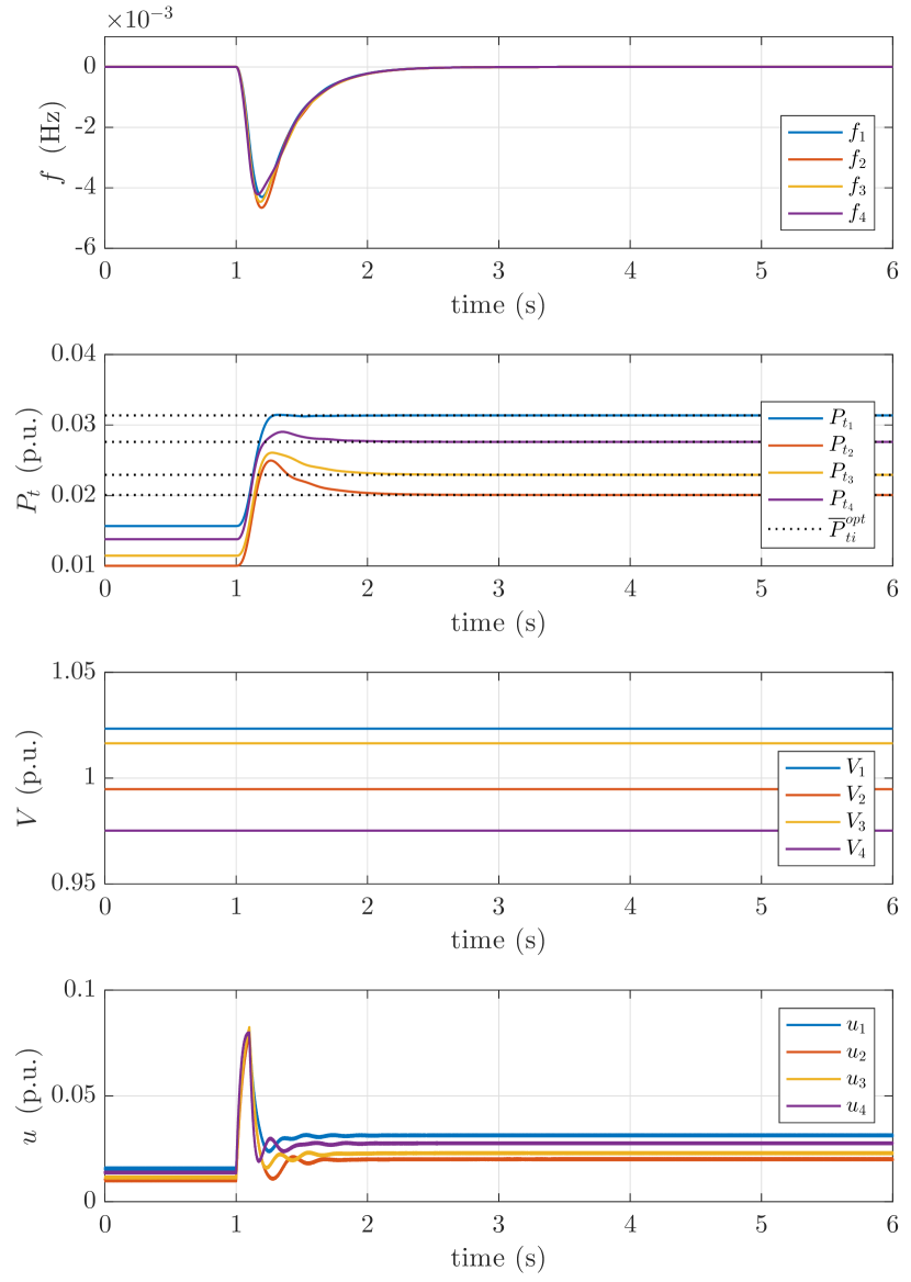
Figure 4: Time evolution of the frequency deviation, generated power, voltage dynamics and control input considering a power demand variation at the time instant $t=$ $1\text{\,}\mathrm{s}$.

In this section, the proposed control solution is assessed in simulation, by implementing a power network partitioned into four control areas (e.g. the IEEE New England 39-bus system [53]). The topology of the power network is represented in Figure 3, together with the communication network (dashed lines).

TABLE II: Network Parameters and Power Demand

		Area 1	Area 2	Area 3	Area 4
$T_{pi}$	(s)	$21.0$	$25.0$	$23.0$	$22.0$
$T_{ti}$	(s)	$0.30$	$0.33$	$0.35$	$0.28$
$T_{gi}$	(s)	$0.080$	$0.072$	$0.070$	$0.081$
$T_{Vi}$	(s)	$5.54$	$7.41$	$6.11$	$6.22$
$K_{pi}$	(Hz p.u.-1)	$120.0$	$112.5$	$115.0$	$118.5$
$R_{i}$	(Hz p.u.-1)	$2.5$	$2.7$	$2.6$	$2.8$
$X_{di}$	(p.u.)	$1.85$	$1.84$	$1.86$	$1.83$
$X^{\prime}_{di}$	(p.u.)	$0.25$	$0.24$	$0.26$	$0.23$
$\overline{E}_{fi}$	(p.u.)	$1.0$	$1.0$	$1.0$	$1.0$
$B_{ii}$	(p.u.)	$-13.6$	$-12.9$	$-12.3$	$-12.3$
$T_{\theta i}$	(s)	$0.33$	$0.33$	$0.33$	$0.33$
$\mathcal{Q}_{i}$	(${10}^{4}$ $ h-1)	$2.42$	$3.78$	$3.31$	$2.75$
$\Delta P_{di}$	(p.u.)	$0.010$	$0.015$	$0.012$	$0.014$

The line parameters are $B_{12}=-5.4$ p.u., $B_{23}=-5.0$ p.u., $B_{34}=-4.5$ p.u. and $B_{14}=-5.2$ p.u., while the network parameters and the power demand $\Delta P_{di}$ of each area are provided in Table II, where a base power of $1000\text{\,}\mathrm{M}\mathrm{W}$ is assumed. The matrices in (27) are chosen as $M_{1}=3I_{4},\,M_{2}=I_{4},\,M_{3}=0.1I_{4}$ and $M_{4}=-(M_{2}+M_{3})$, $I_{4}\in\mathds{R}^{4\times 4}$ being the identity matrix, while the control amplitude $W_{\max_{i}}$ and the parameter $\alpha^{\ast}_{i}$, in (34) are $10$ and $1$, respectively, for all $i\in\mathcal{V}$. For the sake of simplicity, in the cost function (18), we select $\mathcal{R}_{i}=\mathcal{C}_{i}=0$ for all $i\in\mathcal{V}$. The system is initially at the steady state. Then, at the time instant $t=$ $1\text{\,}\mathrm{s}$, the power demand in each area is increased according to the values reported in Table II. From Figure 4, one can observe that the frequency deviations converge asymptotically to zero after a transient where the frequency drops because of the increasing load. Indeed, one can note that the proposed controllers increase the power generation in order to reach again a zero steady state frequency deviation. Moreover, the total power demand is shared among the areas, minimizing the total generation costs. More precisely, by applying the proposed D-SSOSM, the total generation costs are $10$ % less than the generation costs when each area would produce only for its own demand.

VIII Conclusions

A Distributed Suboptimal Second Order Sliding Mode (D-SSOSM) control scheme is proposed to solve an optimal load frequency control problem in power systems. In this work, we adopted a nonlinear model of a power network, including voltage dynamics, where each control area is represented by an equivalent generator including second order turbine-governor dynamics. Based on a suitable chosen sliding manifold, the controlled turbine-governor system, constrained to this manifold, possesses an incremental passivity property that is exploited to prove that the frequency deviation asymptotically approaches zero and an economic dispatch is achieved. Designing the sliding modes, based on passivity considerations, appears to be powerful and we will pursue this approach within different settings, such as achieving power sharing in microgrids. Additionally, we would like to compare the performance of the proposed sliding mode based control scheme with other approaches to OLFC appearing in the literature.

References

- [1] M. Cucuzzella, S. Trip, C. De Persis, and A. Ferrara, “Distributed second order sliding modes for optimal load frequency control,” in Proc. of the 2017 American Control Conference (ACC), Seattle (WA), USA, 2017.
- [2] D. Apostolopoulou, A. D. Domínguez-García, and P. W. Sauer, “An assessment of the impact of uncertainty on automatic generation control systems,” IEEE Transactions on Power Systems, vol. 31, no. 4, pp. 2657–2665, 2016.
- [3] A. M. Ersdal, L. Imsland, and K. Uhlen, “Model predictive load-frequency control,” IEEE Transactions on Power Systems, vol. 31, no. 1, pp. 777–785, Jan. 2016.
- [4] M. Zribi, M. Al-Rashed, and M. Alrifai, “Adaptive decentralized load frequency control of multi-area power systems,” International Jorunal on Electrical Power and Energy Systems, vol. 27, no. 8, pp. 575 – 583, 2005.
- [5] C. Chang and W. Fu, “Area load frequency control using fuzzy gain scheduling of pi controllers,” Electric Power Systems Research, vol. 42, no. 2, pp. 145 – 152, 1997.
- [6] Y. G. Rebours, D. S. Kirschen, M. Trotignon, and S. Rossignol, “A survey of frequency and voltage control ancillary services – part i: Technical features,” IEEE Transactions on Power Systems, vol. 22, no. 1, pp. 350–357, 2007.
- [7] L. L. Lai, Power system restructuring and deregulation: trading, performance and information technology. John Wiley & Sons, 2001.
- [8] D. K. Molzahn, F. Dörfler, H. Sandberg, S. H. Low, S. Chakrabarti, R. Baldick, and J. Lavaei, “A survey of distributed optimization and control algorithms for electric power systems,” IEEE Transactions on Smart Grid, vol. PP, no. 99, pp. 1–1, 2017.
- [9] S. Trip and C. De Persis, “Communication requirements in a master-slave control structure for optimal load frequency control,” in Proc. of the 2017 IFAC World Congress, Toulouse, France, 2017.
- [10] F. Dörfler and S. Grammatico, “Gather-and-broadcast frequency control in power systems,” Automatica, vol. 79, pp. 296 – 305, 2017.
- [11] K. Xi, J. L. Dubbeldam, H. X. Lin, and J. H. van Schuppen, “Power-imbalance allocation control of power systems-secondary frequency control,” arXiv preprint arXiv:1703.02855, 2017.
- [12] X. Zhang and A. Papachristodoulou, “A real-time control framework for smart power networks: Design methodology and stability,” Automatica, vol. 58, pp. 43 – 50, 2015.
- [13] N. Li, C. Zhao, and L. Chen, “Connecting automatic generation control and economic dispatch from an optimization view,” IEEE Transactions on Control of Network Systems, vol. 3, no. 3, pp. 254–264, 2016.
- [14] T. Stegink, C. De Persis, and A. van der Schaft, “A unifying energy-based approach to stability of power grids with market dynamics,” IEEE Transactions on Automatic Control, vol. PP, pp. 1–1, 2016.
- [15] S. You and L. Chen, “Reverse and forward engineering of frequency control in power networks,” in in Proc. 53rd IEEE Conf. on Decision and Control, Los Angeles, CA, USA, Dec. 2014, pp. 191–198.
- [16] A. Kasis, E. Devane, C. Spanias, and I. Lestas, “Primary frequency regulation with load-side participation part I: stability and optimality,” IEEE Transactions on Power Systems, vol. PP, no. 99, pp. 1–1, 2016.
- [17] A. Jokic, M. Lazar, and P. van den Bosch, “Real-time control of power systems using nodal prices,” International Journal of Electrical Power & Energy Systems, vol. 31, no. 9, pp. 522 – 530, 2009.
- [18] R. Mudumbai, S. Dasgupta, and B. B. Cho, “Distributed control for optimal economic dispatch of a network of heterogeneous power generators,” IEEE Transactions on Power Systems, vol. 27, no. 4, pp. 1750–1760, 2012.
- [19] Z. Miao and L. Fan, “Achieving economic operation and secondary frequency regulation simultaneously through local feedback control,” IEEE Trans. Power Syst., vol. PP, no. 99, pp. 1–9, 2016.
- [20] D. Cai, E. Mallada, and A. Wierman, “Distributed optimization decomposition for joint economic dispatch and frequency regulation,” in in Proc. 54th IEEE Conf. on Decision and Control, Dec. 2015, pp. 15–22.
- [21] D. Apostolopoulou, P. W. Sauer, and A. D. Domínguez-García, “Distributed optimal load frequency control and balancing authority area coordination,” in North American Power Symposium (NAPS), 2015, Oct 2015, pp. 1–5.
- [22] P. Yi, Y. Hong, and F. Liu, “Distributed gradient algorithm for constrained optimization with application to load sharing in power systems,” Systems & Control Letters, vol. 83, pp. 45 – 52, 2015.
- [23] ——, “Initialization-free distributed algorithms for optimal resource allocation with feasibility constraints and application to economic dispatch of power systems,” Automatica, vol. 74, pp. 259 – 269, 2016.
- [24] M. Bürger, C. De Persis, and S. Trip, “An internal model approach to (optimal) frequency regulation in power grids,” in Proc. of the 21th International Symposium on Mathematical Theory of Networks and Systems (MTNS), Groningen, the Netherlands, 2014, pp. 577–583.
- [25] S. Trip, M. Bürger, and C. De Persis, “An internal model approach to (optimal) frequency regulation in power grids with time-varying voltages,” Automatica, vol. 64, pp. 240 – 253, 2016.
- [26] J. Schiffer and F. Dörfler, “On stability of a distributed averaging pi frequency and active power controlled differential-algebraic power system model,” in European Control Conf. (ACC), 2016.
- [27] C. Zhao, E. Mallada, and F. Dörfler, “Distributed frequency control for stability and economic dispatch in power networks,” in American Control Conf. (ACC), Jul. 2015, pp. 2359–2364.
- [28] K. Xi, H. X. Lin, C. Shen, and J. H. van Schuppen, “Multi-level power-imbalance allocation control for secondary frequency control in power systems,” arXiv preprint arXiv:1708.03832, 2017.
- [29] N. Monshizadeh, C. De Persis, A. J. van der Schaft, and J. M. A. Scherpen, “A novel reduced model for electrical networks with constant power loads,” arXiv preprint arXiv:1512.08250, abridged version in the Proc. of the 2016 American Control Conference (ACC), 3644- 3649, 2016.
- [30] M. Andreasson, D. V. Dimarogonas, K. H. Johansson, and H. Sandberg, “Distributed vs. centralized power systems frequency control,” in European Control Conf. (ECC), July 2013, pp. 3524–3529.
- [31] S. Kar and G. Hug, “Distributed robust economic dispatch in power systems: A consensus + innovations approach,” in 2012 IEEE Power and Energy Society General Meeting, Jul. 2012, pp. 1–8.
- [32] G. Binetti, A. Davoudi, F. L. Lewis, D. Naso, and B. Turchiano, “Distributed consensus-based economic dispatch with transmission losses,” IEEE Transactions on Power Systems, vol. 29, no. 4, pp. 1711–1720, Jul. 2014.
- [33] N. Rahbari-Asr, U. Ojha, Z. Zhang, and M. Y. Chow, “Incremental welfare consensus algorithm for cooperative distributed generation/demand response in smart grid,” IEEE Trans. Smart Grid, vol. 5, no. 6, pp. 2836–2845, 2014.
- [34] S. Yang, S. Tan, and J. X. Xu, “Consensus based approach for economic dispatch problem in a smart grid,” IEEE Transactions on Power Systems, vol. 28, no. 4, pp. 4416–4426, 2013.
- [35] T. Yang, D. Wu, Y. Sun, and J. Lian, “Minimum-time consensus-based approach for power system applications,” IEEE Transactions on Industrial Electronics, vol. 63, no. 2, pp. 1318–1328, 2016.
- [36] Z. Zhang and M. Y. Chow, “Convergence analysis of the incremental cost consensus algorithm under different communication network topologies in a smart grid,” IEEE Transactions on Power Systems, vol. 27, no. 4, pp. 1761–1768, 2012.
- [37] K. Vrdoljak, N. Perić, and I. Petrović, “Sliding mode based load-frequency control in power systems,” Electrical Power Systems Research, vol. 80, no. 5, pp. 514 – 527, 2010.
- [38] Y. Mi, Y. Fu, D. Li, C. Wang, P. C. Loh, and P. Wang, “The sliding mode load frequency control for hybrid power system based on disturbance observer,” International Journal of Electrical Power and Energy Systems, vol. 74, pp. 446 – 452, 2016.
- [39] G. Bartolini, A. Ferrara, and E. Usai, “Chattering avoidance by second-order sliding mode control,” IEEE Transactions on Automatic Control, vol. 43, no. 2, pp. 241–246, Feb. 1998.
- [40] S. Trip and C. De Persis, “Optimal load frequency control with non-passive dynamics,” IEEE Transactions on Control of Network Systems, vol. PP, no. 99, pp. 1–1, 2017.
- [41] A. Kasis, N. Monshizadeh, E. Devane, and I. Lestas, “Stability and optimality of distributed secondary frequency control schemes in power networks,” arXiv preprint arXiv:1703.00532, 2017.
- [42] J. Machowski, J. Bialek, and D. J. Bumby, Power System Dynamics: Stability and Control, 2nd ed. Wiley, 2008.
- [43] P. Kundur, N. J. Balu, and M. G. Lauby, Power system stability and control. McGraw-hill New York, 1994, vol. 7.
- [44] G. Rinaldi, M. Cucuzzella, and A. Ferrara, “Third order sliding mode observer-based approach for distributed optimal load frequency control,” IEEE Control Systems Letters, vol. 1, no. 2, pp. 215–220, Oct. 2017.
- [45] C. De Persis and N. Monshizadeh, “Bregman storage functions for microgrid control,” arXiv preprint arXiv:1510.05811, 2016.
- [46] L. Bregman, “The relaxation method of finding the common point of convex sets and its application to the solution of problems in convex programming,” USSR Computational Mathematics and Mathematical Physics, vol. 7, no. 3, pp. 200 – 217, 1967.
- [47] P. Kundur, J. Paserba, V. Ajjarapu, G. Andersson, A. Bose, C. Canizares, N. Hatziargyriou, D. Hill, A. Stankovic, C. Taylor, T. V. Cutsem, and V. Vittal, “Definition and classification of power system stability IEEE/CIGRE joint task force on stability terms and definitions,” IEEE Transactions on Power Systems, vol. 19, no. 3, pp. 1387–1401, 2004.
- [48] V. I. Utkin, Sliding Modes in Control and Optimization. Springer-Verlag, 1992.
- [49] A. Levant, “Higher-order sliding modes, differentiation and output-feedback control,” Int. J. Control, vol. 76, no. 9-10, pp. 924–941, Jan. 2003.
- [50] G. Bartolini, A. Ferrara, and E. Usai, “On boundary layer dimension reduction in sliding mode control of uncertain nonlinear systems,” in Proc. of the IEEE Internation Conference on Control Applications, vol. 1, Trieste, Italy, Sep. 1998, pp. 242 –247 vol.1.
- [51] G. P. Incremona, M. Cucuzzella, and A. Ferrara, “Adaptive suboptimal second-order sliding mode control for microgrids,” International Journal of Control, pp. 1–19, Jan. 2016.
- [52] A. Levant, “Sliding order and sliding accuracy in sliding mode control,” International Journal of Control, vol. 58, no. 6, pp. 1247–1263, 1993.
- [53] S. Nabavi and A. Chakrabortty, “Topology identification for dynamic equivalent models of large power system networks,” in Proc. of the 2013 American Control Conference (ACC), Jun. 2013, pp. 1138–1143.