Voltage control of interface rare-earth magnetic moments

Abstract

The large spin orbit interaction in rare earth atoms implies a strong coupling between their charge and spin degrees of freedom. We formulate the coupling between voltage and the local magnetic moments of rare earth atoms with partially filled 4f shell at the interface between an insulator and a metal. The rare earth-mediated torques allow power-efficient control of spintronic devices by electric field-induced ferromagnetic resonance and magnetization switching.

Introduction - The power demand for magnetization control in magnetic memories is an important design parameter. The power consumption of voltage driven magnetization dynamics can be orders of magnitude lower than the one of electric current induced dynamics [1]. In addition, electric voltages are a more localized driving mechanism compared to magnetic fields [1]. From the experimental point of view, magnetization reversal [2; 3] and ferromagnetic resonance [1; 4] driven by electric voltages have been achieved. In those studies, transition-metal films are capped with an insulating barrier that prevents the electric current flow. The main mechanism to couple voltage and magnetization is the control of the perpendicular magnetic anisotropy [5]. Other realizations of the magnetization manipulation by electric fields were conducted in (Ga,Mn)As semiconductor [6] and materials with magnetoelectric properties [7; 8; 13].

The spin-charge coupling that lies beyond the observed phenomena have been modeled by the Rashba [9; 10] and Dzyaloshinskii-Moriya interactions [10; 11; 12], whose origin is the relativistic magnetic field induced by linear momentum of the electron in a transverse electric field. On the other hand, the spin-orbit interaction in central fields of single atoms can best be expressed in terms of the effective magnetic field generated by orbital angular momentum. Here we focus on local magnetic moments in condensed matter system for which the second picture of the spin-orbit interaction is the best starting point.

Local magnetic moments in solids are formed by partially filled $\mathrm{3d}$ and $\mathrm{4f}$ shells of transition metals and rare earths, respectively. The former are relatively light and their spin dynamics are dominated by the exchange interaction, with correction by the crystal fields. Rare earths (RE), on the other hand, have their magnetic sub shell shielded by outer shells, which decreases the effect of crystal-fields and allows the electrons to orbit almost freely in the central Coulomb field of the ionic core with large nuclear charges. The spin-orbit interaction (SOI) of RE is therefore large and free-atomic like. Since SOI couples the electric and magnetic degrees of freedom, we may expect significant effects of electric fields on the RE magnetization dynamics.

Here we study the voltage-driven dynamics of rare earths at the interface between a magnetic insulator (or bad conductor) and a metal. When one of the layers is magnetic, the presence of RE at the interface strongly couples the magnetization to an applied static and dynamic voltage by the local the spin-orbit interaction. Electric fields, applied by high-frequency signal generators for example, are constant inside an insulator but nearly vanish in a metal. The large spatial gradients of the electric field at the interface re-normalize the RE electrostatic interactions with neighboring atoms (crystal-fields), and appear as a voltage modulated magnetic anisotropy and the associated magnetization torque that we derive in the following in more detail.

Magnetism of rare earth ions - In the Russell-Saunders scheme [14] the total spin ($\mathbf{S}$) and orbital ($\mathbf{L}$) momenta are the sum of the single electron momenta of the $\mathrm{4f}$-orbitals $\mathbf{S}=\sum_{j}\mathbf{s}_{j}$ and $\mathbf{L}=\sum_{j}\mathbf{l}_{j}$. The spin-orbit coupling reads $H_{\mathrm{SOI}}=\Lambda\mathbf{S}\cdot\mathbf{L}$, and the coupling parameter $\Lambda$ is positive (negative) for less (more) than half-filled sub shell [14; 15]. The total angular momentum vector $\mathbf{J}=\mathbf{S}+\mathbf{L}$ and the angular part of the eigenfunctions can be written as $|\Psi\rangle=|S,L,J,J_{z}\rangle$, where the quantum numbers are governed by $\mathbf{S}^{2}|\Psi\rangle=\hbar^{2}S(S+1)|\Psi\rangle$, $\mathbf{L}^{2}|\Psi\rangle=\hbar^{2}L(L+1)|\Psi\rangle$, $\mathbf{J}^{2}|\Psi\rangle=\hbar^{2}J(J+1)|\Psi\rangle$, $\hat{J}_{z}|\Psi\rangle=\hbar J_{z}|\Psi\rangle$, $\hat{J}_{z}$ is the $z$-component of the vector $\mathbf{J,}$ and $\hbar$ is Planck’s constant divided by $2\pi$. The lowest-energy state of RE ions as governed by Hund’s rules [14] are listed in Table 1. The Wigner-Eckart theorem ensures that within this ground state manifold the angular momenta are collinear, viz. $\mathbf{S}=(g_{J}-1)\mathbf{J}$ and $\mathbf{L}=(2-g_{J})\mathbf{J}$ in terms of the Landé g-factor $g_{J}$. Furthermore, for constant $(S,L,J)$ the orbital symmetry axis and the spin vector move rigidly together, implying a strong spin-charge coupling [16; 17].

Ion	$4f^{n}$	S	L	J	Shape	$Q_{2}/a_{0}^{2}$
Ce3+	$4f^{1}$	$\frac{1}{2}$	3	$\frac{5}{2}$	Oblate	-0.686
Pr3+	$4f^{2}$	1	5	4	Oblate	-0.639
Nd3+	$4f^{3}$	$\frac{3}{2}$	6	$\frac{9}{2}$	Oblate	-0.232
Pm3+	$4f^{4}$	2	6	4	Prolate	0.202
Sm3+	$4f^{5}$	$\frac{5}{2}$	5	$\frac{5}{2}$	Prolate	0.364
Eu3+	$4f^{6}$	3	3	0	-	-
Gd3+	$4f^{7}$	$\frac{7}{2}$	0	$\frac{7}{2}$	Spherical	0
Tb3+	$4f^{8}$	3	3	6	Oblate	-0.505
Dy3+	$4f^{9}$	$\frac{5}{2}$	5	$\frac{15}{2}$	Oblate	-0.484
Ho3+	$4f^{10}$	2	6	8	Oblate	-0.185
Er3+	$4f^{11}$	$\frac{3}{2}$	6	$\frac{15}{2}$	Prolate	0.178
Tm3+	$4f^{12}$	1	5	6	Prolate	0.427
Yb3+	$4f^{13}$	$\frac{1}{2}$	3	$\frac{7}{2}$	Prolate	0.409

Table 1: Ground state $(S,L,J)$ based on Hund’s rules and shape of the $4f$ ground state electron density [16]. $Q_{2}$ is the quadrupole moment calculated using the Wigner-Eckart theorem for the state $J_{z}=J$, and $a_{0}=0.53$ Å is the Bohr radius. The Wigner-Eckart theorem cannot be applied to Eu because $\mathbf{J}=0$.

The electron density of a partially filled $\mathrm{4f}$ sub shell can be written as

$$n_{\mathrm{4f}}(\mathbf{r})=\sum_{m_{l}=-3}^{3}|R_{\mathrm{4f}}(r)Y_{3}^{m_{l}}(\mathbf{\hat{r}})|^{2}\left(f_{m_{l}\uparrow}+f_{m_{l}\downarrow}\right),$$ (1)

where $\mathbf{r}=r\mathbf{\hat{r}}$ is the position vector in spherical coordinates, $R_{\mathrm{4f}}(r)$ the radial part of the $\mathrm{4f}$ atomic-like wave function, and the spherical harmonics $Y_{3}^{m_{l}}(\mathbf{\hat{r}})$ describe the angular dependence. $f_{m_{l},m_{s}}$ is the occupation number of the single electron state with magnetic quantum numbers of orbital $m_{l}$ and spin $m_{s}$ angular momenta. The density $n_{\mathrm{4f}}$ is normalized to the number of electrons in the $\mathrm{4f}$ shell $N_{\mathrm{4f}}=\int n_{\mathrm{4f}}(\mathbf{r},t)d\mathbf{r}$. The typical $\mathrm{4f}$ radius, $\langle r\rangle\sim 0.5$ Å, is much smaller than typical inter atomic distances, $R\sim 3$ Å, which motivates the multipole expansion [16; 17]

$$n_{\mathrm{4f}}(\mathbf{r})\approx\frac{|R_{\mathrm{4f}}(r)|^{2}}{4\pi}\left\{N_{\mathrm{4f}}+\frac{5Q_{2}}{4\langle r^{2}\rangle}\left[3\left(\mathbf{m}\cdot\mathbf{\hat{r}}\right)^{2}-1\right]\right\},$$ (2)

where $Q_{2}\equiv\int\left(3z^{2}-r^{2}\right)n_{\mathrm{4f}}(\mathbf{r})d\mathbf{r}$ is the quadrupole moment listed in Table 1. $\mathbf{m}=-\mathbf{J}/|\mathbf{J}|$ is the unit magnetization vector that at equilibrium is taken to be $\mathbf{e}_{z}$ but in an excited state may depend on time. The unit position vector in spherical coordinates is $\mathbf{\hat{r}}=\sin\theta\left[\mathbf{e}_{x}\cos\phi+\mathbf{e}_{y}\sin\phi\right]+\mathbf{e}_{z}\cos\theta$, where $\{\mathbf{e}_{x},\mathbf{e}_{y},\mathbf{e}_{z}\}$ are the unit vectors along the Cartesian axes. For $Q_{2}>0$ $\left(Q_{2}<0\right)$ the envelope function of the electron density is a pancake or cigar-like (oblate or prolate) ellipsoid, respectively.

A local magnetic ion interacts weakly with static electric fields, $\mathbf{E}=-\nabla V$, where $V$ is the voltage or potential energy of a positive probe charge. To leading order, the ions experience the electrostatic energy [18]

$$\langle\psi|-e\sum_{i=1}^{N_{\mathrm{4f}}}V(\mathbf{r}_{i})|\psi\rangle=-e\int d^{3}rV(\mathbf{r})n_{\mathrm{4f}}(\mathbf{r}),$$ (3)

where $-e$ is the electron charge, and $-eV(\mathbf{r}_{i})$ is the potential energy of the $i$-th electron. $|\psi\rangle$ is the $\mathrm{4f}$ many-electron wave function in the ground state. Again, the leading order in a multipole expansion of the crystal field around the origin $\mathbf{r}=0$ can be parameterized by a quadrupolar term $A_{2}^{(0)}$

$$eV(\mathbf{r})=-A_{2}^{(0)}r^{2}\left(3\cos^{2}\theta-1\right).$$ (4)

Inserting Eqs. (2) and (4) into Eq. (3), we arrive at a Hamiltonian that depends on the magnetization direction as

$$H_{\mathrm{ani}}=\frac{3}{2}Q_{2}A_{2}^{(0)}m_{z}^{2}.$$ (5)

The crystal symmetry orients here the easy ($Q_{2}A_{2}^{(0)}<0$) or hard ($Q_{2}A_{2}^{(0)}>0$) magnetic axis along the $z$ direction. This crystal field  energy accounts for the single rare-earth ion magnetic anisotropy. The parameter $A_{0}^{(2)}$ can be calculated by first principles or to fit to experiments. Typical values are: $A_{0}^{(2)}=300$ $\mathrm{K}a_{0}^{-2}$ for (RE)₂Fe₁₄B, $A_{0}^{(2)}=34$ K$a_{0}^{-2}$ for (RE)₂Fe₁₇, and $A_{0}^{(2)}=-$358 K $a_{0}^{-2}$ for (RE)₂Fe₁₇N₃ [17], where $a_{0}=0.53$ Å is the Bohr radius. The origin of the strong magnetic anisotropy of REs is their large spin-orbit interactions. On the other hand, for $3d$ transition metal moments, the anisotropy is usually very small, except at interfaces, where the orbital motions are partially unquenched. In such cases, the anisotropy emerges as the consequence of SOI, the quadrupolar shape of electric potentials at the interface [5], the hybridization of orbitals and change in the orbitals occupation.

At an interface between materials with different work functions the symmetry is reduced by potential steps. The electric field exhibits spatial gradients due to charge accumulation immediately at the interface that result in a step potential. An external voltage difference $\Delta V$ drops only over the insulator, but is constant in the metal (when the ferromagnet is a bad conductor the effects are weaker but still exist). The electric field therefore depends on position in the immediate proximity of the interface. This dependence electric field gradients can interact with the 4f sub shell as an effective crystal field.

Voltage coupling at interfaces - Let us focus on a magnetic insulator film with thickness $L_{F}$. At the surface, the insulator exposes $n_{\mathrm{RE}}$ rare earth moments per unit of area. Inside the insulator, the electric field is approximately constant, $\mathbf{E}(z<0)=\mathbf{e}_{z}\Delta V/L_{F}$, while it vanishes in the metal $\mathbf{E}(z>0)=0$, see Fig. 1a). Using Eq. (3), the electric energy of a magnetic moment at the origin is then

$$H_{e}=H_{0}-\frac{15}{64}\frac{e\Delta V}{L_{F}}Q_{2}\frac{\langle r\rangle}{\langle r^{2}\rangle}m_{z}^{2}$$ (6)

where $H_{0}=5eE_{0}Q_{2}\langle r\rangle/(64\langle r^{2}\rangle)+e(\Delta V/L_{F})N_{\text{{4f}}}\langle r\rangle/4$ does not depend on the magnetization and $\langle r^{n}\rangle\equiv N_{\mathrm{4f}}^{-1}\int r^{n}n_{\text{{4f}}}(\mathbf{r})d\mathbf{r}$. In the Supplement [25] different approaches to formulate the coupling yield expressions similar to Eq. (6). For $\langle r^{2}\rangle^{1/2}\sim\langle r\rangle\sim 0.5$ Å the coupling energy per unit area at equilibrium ($m_{z}^{2}=1$)

$$\left|n_{\mathrm{RE}}(H_{e}-H_{0})\frac{L_{F}}{\Delta V}\right|=750\frac{\mathrm{fJ}}{\mathrm{Vm}}\frac{Q_{2}}{10^{-3}\mathrm{nm}^{2}}\frac{n_{\mathrm{RE}}}{\mathrm{nm}^{-2}}$$ (7)

is one order of magnitude larger than the corresponding coupling in transition metals [21; 22]. For electric fields $\Delta V/L_{F}\sim 10$ mV/nm $=100$ kV/cm, the surface energy density becomes $(H_{e}-H_{0})n_{\mathrm{RE}}\approx 7.5\times 10^{-3}$ erg/cm${}^{2}=7.5\,\mathrm{\mu}$J/m².

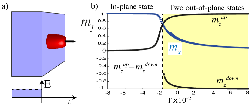
Figure 1: Spin-charge coupling for an interface local magnetic moment. a) Electric field at an interface between an insulator (constant electric field) and a metal (vanishing electric field). The magnetic dipole and charge quadrupole at the interface are strongly coupled. b) Ground state magnetization directions $\mathbf{m}=(m_{x},m_{y},m_{z})$ as a function of interface electric field with coupling parameter $\Gamma$ [Eq. (9)] and a magnetic field tilted from the z-axis by an angle $\varphi\sim 6^{\circ}$. The system switches from a perpendicular easy axis to an easy-plane configuration for $\Gamma<0.018.$

The step field model can also be applied to non-magnetic insulators$|$transition-metal ferromagnets (such as Fe, Co, and Ni, or their alloys) with RE ions at the interface that are antiferromagnetically coupled to the magnetic order [23; 24] and facilitate a large coupling of the magnetization to electric fields. Good insulators, such as MgO, can endure very large electric fields (of the order of $300$ mV/nm, in FeCo$|$MgO, Ref. [21], for example). Thus, MgO based magnetic tunnel junctions with rare earth doping or dusting are promising devices to study and apply electric field-induced modulations of the magnetization configuration.

In magnetic materials, local angular momenta are strongly locked by the exchange interaction. When a sufficiently strong static magnetic field $\mathbf{B}$ is applied, the macrospin model is valid, i.e. the magnetization $\mathbf{M}$ is constant in space. The total magnetic energy $H_{M}$ per unit area then reads

$$\frac{H_{M}}{\mu_{0}M_{s}^{2}L_{F}}=-\mathbf{m}\cdot\mathbf{h}-\frac{\beta_{x}}{2}m_{x}^{2}+\frac{\beta_{z}-\Gamma}{2}m_{z}^{2}.$$ (8)

The first term on the (dimensionless) right-hand side with $\mathbf{h}=\mathbf{B/}\left(\mu_{0}M_{s}\right)$ is the Zeeman energy and $M_{s}$ the saturation magnetization. The parameters $\beta_{x}$ ($\beta_{z}$) account for the in-plane (out of plane) magnetic anisotropy in the absence of applied electric fields, $\Delta V=0$. The dimensionless coupling parameter $\Gamma$ measures the relative strength of the electrostatic coupling $\sim n_{\mathrm{RE}}e\Delta VQ_{2}/L_{F}$ that should be compared with magnetic anisotropies. $\Gamma\sim 0.06$ with the following parameters representative for a rare earth iron garnet thin film such as Tm₃Fe₅O₁₂

$$\Gamma=0.06\frac{n_{\mathrm{RE}}}{1/\mathrm{nm}^{2}}\left(\frac{10^{5}\mathrm{A/m}}{M_{s}}\right)^{2}\left(\frac{10\,\mathrm{nm}}{L_{F}}\right)^{2}\frac{\Delta V}{0.1\,\mathrm{V}}\frac{Q_{2}}{10^{-3}\mathrm{nm}^{2}}$$ (9)

Since the $M_{s}$ of 8 nm thick Tm₃Fe₅O₁₂ [19] is at room temperature about 10 times smaller than that of even a subnanometer FeCo film [21], the coupling strength $\Gamma$ is 10 times larger for magnetic insulators for the same applied electric field without the need for additional tunnel barriers. Intraband transition and electric breakdown is of no concern as long as $eE_{0}\ll\epsilon_{\mathrm{gap}}^{2}/(\epsilon_{F}a)$, where $\epsilon_{\mathrm{gap}}$ is the band gap, $\epsilon_{F}$ is the Fermi level in the metal and $a$ the lattice constant [26]. Using $\epsilon_{F}\sim 2$ eV, and the gap/lattice constant for yttrium iron garnet (YIG) [27; 28] $\epsilon_{\mathrm{gap}}\sim 2.85$ $\mathrm{eV}$/$a=1.2$ nm, we estimate $E_{0}\ll 2$ $\mathrm{V}$/nm to be safe. The coupling strength $\Gamma$ decreases $\sim L_{F}^{-2}$ for a given voltage, so much can be gained by choosing an insulator with a large gap and breakdown voltage that permits working with thin layers.

Figure 1b) shows the stable magnetizations that minimize of the energy (8) in the presence of a magnetic field $\mathbf{h}=h[\mathbf{e}_{x}\cos\varphi+\mathbf{e}_{z}\sin\varphi]$ that is tilted by an angle $\varphi.$ The parameter are $h=0.01$, $\varphi=5.72^{\circ}$, $\beta_{x}=0$, $\beta_{z}=-0.03$. The application of a constant voltage allows the transition from the easy axis (right zone) to the easy plane (left zone) configuration.

The electric field effects in transition metal devices as well as one proposed here, derive from the same type of magnetic anisotropy, although the microscopic coupling mechanism is different. The phenomenology of electric field-induced precessional dynamics as observed in transition metal systems [30] does not differ from the one we expect for RE systems. The advantage of interface REs is the lower power consumption and the possibility of using a wider range of materials including magnetic insulators, such as YIG. The magnetization dynamics is described by the Landau-Lifshitz-Gilbert equation,

$$\dot{\mathbf{m}}=-\gamma\mathbf{m}\times\mathbf{h}_{\mathrm{eff}}+\alpha\mathbf{m}\times\dot{\mathbf{m}},$$ (10)

where $\alpha$ is Gilbert damping constant, $\gamma>0$ is the (modulus of the) gyromagnetic ratio, $\dot{\mathbf{m}}$ the temporal derivative of $\mathbf{m}$, and the effective magnetic field $\mathbf{h}_{\mathrm{eff}}$ satisfying

$$\frac{\mathbf{h}_{\mathrm{eff}}}{\mu_{0}M_{s}}\equiv\frac{1}{\mu_{0}M_{s}^{2}L_{F}}\frac{\partial H_{M}}{\partial\mathbf{m}}=\mathbf{h}+\beta_{x}m_{x}\mathbf{e}_{x}+\left[\Gamma-\beta_{z}\right]m_{z}\mathbf{e}_{z}.$$ (11)

The magnetic torque exerted by the electric field is proportional to $-\mathbf{m}\times\gamma m_{z}\mathbf{e}_{z}$.

Ferromagnetic resonance - We now turn to an ac electric field that modulates the coupling $\Gamma=\Gamma_{0}\cos(\Omega t)$, with frequency $\Omega$ close to the ferromagnetic resonance (GHz). Since the electric field is normal to thin metallic films $<100$ nm, the induced Oersted-like magnetic field and associated power are negligibly small. In linear response the model (10) can be solved analytically for $\beta_{x}=\beta_{z}=0$. The polar coordinate system is spanned by the unit vectors $\mathbf{e}_{1}=\mathbf{e}_{x}\cos\left(\varphi\right)+\mathbf{e}_{z}\sin\varphi$, $\mathbf{e}_{2}=-\mathbf{e}_{x}\sin\left(\varphi\right)+\mathbf{e}_{z}\cos\varphi$, and $\mathbf{e}_{3}=-\mathbf{e}_{y}$. At equilibrium state $\mathbf{m}_{\mathrm{eq}}=\mathbf{e}_{1}$ along the applied magnetic field. Around the equilibrium state, the magnetization is $\mathbf{m}=\mathbf{e}_{1}+\delta\mathbf{m}$, where $\delta\mathbf{m}=\delta m_{2}\mathbf{e}_{2}+\delta m_{3}\mathbf{e}_{3}$ is the deviation from $\mathbf{m}_{\mathrm{eq}}$, with $\left|\delta\mathbf{m}\right|\ll 1$ and $\delta\mathbf{m}\cdot\mathbf{m}_{\mathrm{eq}}=0$. To leading order in the coupling ($\Gamma_{0}$) and dissipation ($\alpha$), the effective field is $(\mu_{0}M_{s})^{-1}\mathbf{h}_{\mathrm{eff}}=h\mathbf{e}_{1}+\Gamma\cos(\Omega t)\sin(\varphi)\left[\mathbf{e}_{1}\sin(\varphi)+\mathbf{e}_{2}\cos\varphi\right]$ and

$$\frac{\delta\dot{\mathbf{m}}}{\omega_{M}}=\mathbf{e}_{1}\times\left[h\delta\mathbf{m}+\alpha\frac{\delta\dot{\mathbf{m}}}{\omega_{M}}-\frac{\Gamma_{0}}{2}\cos(\Omega t)\sin(2\varphi)\mathbf{e}_{2}\right],$$

where $\omega_{M}\equiv\gamma\mu_{0}M_{s}$. The effective ac magnetic field $\mathbf{B}_{\mathrm{ac}}=\mu_{0}M_{s}\Gamma_{0}\sin(2\varphi)\cos(\Omega t)\mathbf{e}_{z}/2$. Then

$$\delta\mathbf{m} =(\Gamma_{0}/4)\sin(2\varphi)\chi^{\prime}(\Omega)\left(\cos(\Omega t)\mathbf{e}_{2}+\sin(\Omega t)\mathbf{e}_{3}\right)$$

$$+(\Gamma_{0}/4)\sin(2\varphi)\chi^{\prime\prime}(\Omega)\left(\sin(\Omega t)\mathbf{e}_{2}-\cos(\Omega t)\mathbf{e}_{3}\right),$$

where $\chi^{\prime}$ and $\chi^{\prime\prime}$ are the real and imaginary parts of the dynamics susceptibility

$$\chi(\omega)\equiv\frac{\omega_{M}\left(\omega_{0}-\omega\right)}{\left(\omega_{0}-\omega\right)^{2}+\omega^{2}\alpha^{2}}+i\frac{\omega_{M}\alpha\omega}{\left(\omega_{0}-\omega\right)^{2}+\omega^{2}\alpha^{2}},$$

and the natural frequency is $\omega_{0}\equiv\omega_{M}h=\gamma\mu_{0}M_{s}h$. Figure 2 illustrates $\delta\mathbf{m}(t)$ (continuous lines) together with the numeric solution (dots). We see that a large oscillation cone $\left|\delta\mathbf{m}\right|\sim 0.15$ can be achieved by a relatively low voltage for the aforementioned parameter values and $\Gamma_{0}=0.01$ (or $\Delta V/L_{F}\sim 1.6$ $\mathrm{mV/nm}$).

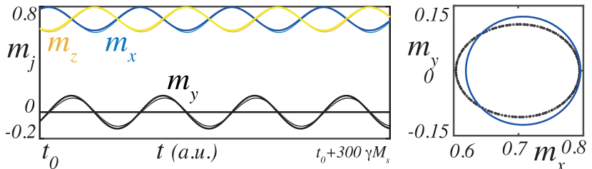
Figure 2: (a) Magnetization dynamics induced by time-varying voltages. Comparison between analytic (solid line) and (b) numeric (dot) precessional (FMR) solutions, obtained for $\Gamma=\Gamma_{0}\cos(\Omega t)$, $\Gamma_{0}=0.01$, $\beta_{x}=\beta_{z}=0$, $\Omega=0.08$, $h=0.1$, $\varphi=45^{\circ}$, and $\alpha=0.005$.

Magnetization switching - Magnetic reversal in tunnel junctions is the key process in magnetic random access memories. An applied voltage can reduce the energy barrier for magnetic field and current-induced switching or directly trigger the magnetization reversal [30]. The latter effect is illustrated by Fig. 3 assuming perpendicular magnetization (for in-plane magnetization, see Ref. [2; 3]). An equilibrium magnetization along $z$ [either an up or down state in the right zone of Fig. 1b)] is excited by a step-like voltage pulse into large damped precessions around the in-plane equilibrium [left zone of Fig. 1b)]. When the voltage is turned off again at the right time, the magnetization can be fully reverted. The switching is observed with large tolerance in the pulses duration between the pico and nano second scales. In the simulation of Fig. 3, the pulse duration is around 1 ns, while the application of subsequent pulses toggles the magnetization direction faithfully.

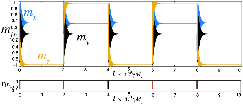
Figure 3: Precessional switching for an easy axis perpendicular magnet ($\beta_{z}=-0.03$) induced by a voltage box train. Up pannel shows the magnetization components, while the low panel shows the box consisting of a negative voltage with $\Gamma=-0.03$ for $\Delta t=$ $4000\gamma M_{s}$ ($\sim$ 1 ns) followed by $\Gamma=0$. This signal is repeated all $2\times 10^{5}\gamma M_{s}$ ($\sim$25 ns). Other parameters are $\beta_{x}=0$, $h=0.01$, $\varphi=5.72^{\circ}$, and $\alpha=0.005$.

Conclusions and remarks - We report voltage-modulated magnetic anisotropies and magnetization dynamics of rare-earth magnetic moments at insulator$|$metal bi-layer interfaces. An applied voltage generates inhomogenous electric fields at interfaces with large conductivity mismatch that couple efficiently to rare earth ions with non-spherical electron distributions, which is usually the case when the shell is not half or completely filled. The dynamics of the charge and spin distributions are locked by the spin-orbit interaction. The voltage can then rigidly precess the charge and spin distributions of the entire $\mathrm{4f}$ sub shell via a stronger and direct coupling to the spin than in transition metals. Adding rare-earth impurities to insulator$|$metal bi-layers can be used to efficiently switch the magnetization and induce ferromagnetic resonance. Future applications may include rare earth-dusted magnetic insulator$|$normal metal interfaces, such as YIG$|$Pt, that can efficiently convert an ac voltage into a spin current by spin-pumping.

Acknowledgments.- We acknowledge the financial support from JSPS KAKENHI Grants Nos. 25247056, 25220910, and 26103006 and JSPS Fellowship for Young Scientists No. JP15J02585. We profited from initial research by Dr. Mojtaba Rahimi.

Supplemental Material to Voltage control of interface rare-earth magnetic moments

This supplemental material shows alternative derivations of the coupling between voltage and rare earth magnetic moments. Details on the numerical simulation of the voltage-induced dynamics are also presented.

I Rare earth impurities at a metal interface

Here we describe the insulator$|$magnetic metal bi-layer in terms of a screening-induced crystal field shift, which is a Thomas-Fermi-like justification of the step model used in the main text. The electric field in a metal normal to the interface to an insulator (in the $x-y$ plane) reads in a local screening model

$$\mathbf{E}(z)=E_{0}e^{-z/d_{\mathrm{TF}}}\mathbf{e}_{z},$$ (S1)

where $E_{0}$ is the electric field in the insulator and $d{{}_{\mathrm{FT}}}$ is the Thomas-Fermi screening length. Figure S1 illustrates the electric field profile. For a non-magnetic metal $d{{}_{\mathrm{FT}}}\equiv[\epsilon_{0}/(e^{2}g)]^{1/2}$, where $g$ is the conduction electron density of states at Fermi level and $\epsilon_{0}$ is the permittivity of free space. In ferromagnetic metals, $d{{}_{\mathrm{TF}}}$ can be obtained using Poisson equation and a Stoner model (see Ref. [1]). For elemental metals the screening length of the order of an Å. For example, for Fe(bcc), $d{{}_{\mathrm{TF}}}=1.3$ Å [1]. In close proximity of a given atom we have then a modified “crystal field” that can be expressed by the leading terms of a Taylor expansion

$$\mathbf{E}(z) \approx E_{0}\mathbf{e}_{z}+\left(\frac{\partial E}{\partial z}\right)_{0}z\mathbf{e}_{z}=-\mathbf{e}_{z}\frac{\partial}{\partial z}\left[-E_{0}z-\frac{1}{2}\left(\frac{\partial E}{\partial z}\right)_{0}z^{2}\right],$$

$$=-\mathbf{e}_{z}\frac{\partial}{\partial z}\left[-E_{0}z-\frac{1}{6}\left(\frac{\partial E}{\partial z}\right)_{0}\left(3z^{2}-r^{2}\right)-\frac{1}{6}\left(\frac{\partial E}{\partial z}\right)_{0}r^{2}\right].$$ (S2)

The potential near the interface has dipolar [$-E_{0}z$], an isotropic [$-(1/6)\left(\partial_{z}E\right)_{0}r^{2}$] and uni-axial [quadrupolar: $-(1/6)\left(\partial_{z}E\right)_{0}(3z^{2}-r^{2})$] contributions. The latter can be estimated from Eq. (S1) close to $z=0$,

$$V(\mathbf{r})=\frac{r^{2}E_{0}}{6d{{}_{\mathrm{TF}}}}\left(3\cos^{2}\theta-1\right),$$ (S3)

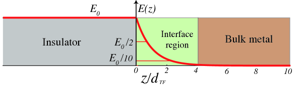
Figure S1: (Color online) Interface screening. The electric field is finite inside the insulator and vanishes deeper inside the metal. At the interface, the charge accumulation generates gradients in the electric field and potential. Only inside the metal and very close to the interface (interface region) the rare earth ions is affected by an applied electric voltage.

which corresponds to the magnetic anisotropy energy

$$H_{\mathrm{ani},M}=-\frac{eQ_{2}}{4d{{}_{\mathrm{TF}}}}E_{0}m_{z}^{2},$$ (S4)

where $m_{z}$ is the unit magnetization component along the interface normal ($m_{z}=\mathbf{m}\cdot\mathbf{e_{z}}$), and $Q_{2}\equiv\int\left(3z^{2}-r^{2}\right)n_{\mathrm{4f}}(\mathbf{r})d\mathbf{r}$ is quadrupolar moment of the rare earth ion. For typical values $d_{TF}\sim 10^{-1}$ nm and $Q_{2}\sim 10^{-3}$ nm², this energy is of the same order of magnitude as the one obtained for the simple step model in the main text [Eq. (6)].

II Torque derivation using Newtonian mechanics

The strong spin-charge coupling in rare earth atoms implies also the locking between the atom angular momentum and the $4f$ sub shell mass distribution. This property allows us to derive the torque exerted by voltages using the simple approach of the Newtonian mechanics, which we present below for the non-specialist reader.

The force acting on a charge element $dQ=-en_{\mathrm{4f}}(\mathbf{r})d^{3}r$ of volume element $d\mathbf{r}$ at $\mathbf{r}$ is

$$d\mathbf{F}(\mathbf{r})=-en_{\mathrm{4f}}(\mathbf{r})\mathbf{E}(\mathbf{r})d\mathbf{r},$$ (S5)

The corresponding (mechanical) torque is

$$\mathbf{T_{m}}=\int\mathbf{r}\times d\mathbf{F}(\mathbf{r})=-e\int n_{\mathrm{4f}}(\mathbf{r})\mathbf{r}\times\mathbf{E}(\mathbf{r})d\mathbf{r},$$ (S6)

and it acts on a non-spherical electron distribution as parameterzed by the quadrupole moment $Q_{2}$ and oriented along the unit vector $\mathbf{m}$. Expanding the electric field in a Taylor series near the origin, $\mathbf{E}(\mathbf{r})=[E_{0}+z(\partial E/\partial z)_{0}]\mathbf{e_{z}}$

$$\mathbf{T_{m}} =\frac{e\langle r^{2}\rangle}{4\pi}\left(\frac{\partial E}{\partial z}\right)_{0}\mathbf{e}_{z}\times\int_{0}^{\pi}d\theta\sin(\theta)\cos(\theta)\int_{0}^{2\pi}d\phi\mathbf{\hat{r}}\left[N_{4f}+\frac{5Q_{2}}{4\langle r^{2}\rangle}\left(3\left[\mathbf{m}(t)\cdot\frac{\mathbf{r}}{r}\right]^{2}-1\right)\right],$$ (S7)

$$=-\frac{eQ_{2}}{2}\left(\frac{\partial E}{\partial z}\right)_{0}\left(\mathbf{m}\cdot\mathbf{e}_{z}\right)\mathbf{m}\times\mathbf{e}_{z}=\mathbf{m}\times\frac{\delta}{\delta\mathbf{m}}\left[-\frac{eQ_{2}}{4}\left(\frac{\partial E}{\partial z}\right)_{0}\left(\frac{M_{z}}{M_{s}}\right)^{2}\right].$$ (S8)

The orbital and magnetic (classical) momenta are related by the gyromagnetic ratio $-\gamma$ (where $\gamma>0$). The mechanical torque $\mathbf{T_{m}}$ is therefore proportional to the magnetic torque $\mathbf{T}:$

$$\mathbf{T}=\gamma\frac{eQ_{2}}{2}\left(\frac{\partial E}{\partial z}\right)_{0}\left(\mathbf{m}\cdot\mathbf{e}_{z}\right)\mathbf{m}\times\mathbf{e}_{z}$$

which enters the Landau-Lifshitz-Gilbert equation.

III Numerical simulations

The dimensionless Landau-Lifshitz-Gilbert equation, $\dot{\mathbf{m}}=-\mathbf{m}\times\mathbf{h}_{\mathrm{eff}}+\alpha\mathbf{m}\times\dot{\mathbf{m}}$, decomposed in Cartesian coordinates and written in the Landau-Lifshitz form:

$$(1+\alpha^{2})\frac{dm_{x}}{dt} =\alpha m_{x}\left(m_{z}^{2}\left[\beta_{x}+\beta_{z}-\Gamma\right]+\beta_{x}m_{y}^{2}\right)+(\beta_{z}-\Gamma)m_{y}m_{z}$$

$$-h\sin(\varphi)(\alpha m_{x}m_{z}+m_{y})+\alpha h\cos(\varphi)\left(m_{y}^{2}+m_{z}^{2}\right),$$

$$(1+\alpha^{2})\frac{dm_{y}}{dt} =-\beta_{x}m_{x}(\alpha m_{x}m_{y}+m_{z})+m_{z}\left[\beta_{z}-\Gamma\right](\alpha m_{y}m_{z}-m_{x})$$

$$+h\sin(\varphi)(m_{x}-\alpha m_{y}m_{z})-h\cos(\varphi)(\alpha m_{x}m_{y}+m_{z}),$$

$$(1+\alpha^{2})\frac{dm_{z}}{dt} =-\alpha m_{z}\left(\beta_{x}m_{x}^{2}+\left[\beta_{z}-\Gamma\right]\left(m_{x}^{2}+m_{y}^{2}\right)\right)+\beta_{x}m_{x}m_{y}$$

$$+\alpha h\sin(\varphi)\left(m_{x}^{2}+m_{y}^{2}\right)+h\cos(\varphi)(m_{y}-\alpha m_{x}m_{z}).$$ (S9)

which is rendered dimensionless by measuring time in units of $\left(\gamma M_{s}\right)^{-1}$. We solve set of Eqs. (S9) by using a fifth order Runge-Kutta scheme based on Ref. [2]. A time step of $\Delta t=0.01$ [in units of $(\gamma M_{s})^{-1}$] is sufficiently small for accurate results. We monitored norm conservation, by requiring $\left|1-(m_{x}^{2}+m_{y}^{2}+m_{z}^{2})^{1/2}\right|\leq 10^{-6}$. The graphs in the main text were plotted after integrating the equation of motion for a transient time of order $t_{0}=10^{5}$. Unless mentioned explicitly, the resulting dynamics does not depend on the initial condition.

III.1 Stationary states of the LLG equation

The stationary state ($\dot{\mathbf{m}}=0$) in the presence of a constant applied voltage as parameterized by $\Gamma$ should satisfy $\mathbf{m}\times\mathbf{h_{\mathrm{eff}}}=0$, or

$$\mathbf{m}=\left(\frac{h\cos(\varphi)}{\lambda-\beta_{x}},0,\frac{h\sin(\varphi)}{\lambda+\beta_{z}-\Gamma}\right),$$ (S10)

where the $\lambda$ is obtained from the normalization condition $\left|\mathbf{m}\right|=1$. By integrating the set of equations (S9) for different initial conditions, we obtain the shifted equilibrium states, as shown in Fig. 1 of the main text.

III.2 Ferromagnetic resonance

As oscillating voltage $\Gamma(t)=\Gamma_{0}\cos(\Omega t)$ leads to resonance, as illustrated in Figure S2 for two different voltage amplitudes, and Fig. S3 shows the precession cone as function of the angle. Large oscillations ($|\delta\mathbf{m}|$ of about 10% of $M_{s}$) can be achieved for relatively low values of the spin-charge coupling parameter ($\Gamma_{0}\sim 0.01$)

!

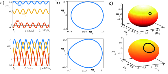
Figure S2: (Color online) Voltage induced ferromagnetic resonance. The up and down panels show the ac electric field- induced steady-state magnetization dynamics calculated for coupling parameters $\Gamma_{0}=0.01$ and $\Gamma_{0}=0.05$, respectively. a) Cartesian components as function of time. b) Phase portrait of the variables $(m_{x},m_{y})$. c) Precession cone on the unit sphere $\mathbf{m}^{2}=1$. Other parameters are $\Omega=0.08$, $h=0.1$, $\phi=45^{\circ}$, $\beta_{x}=0.001$, $\beta_{z}=0.05$ and $\alpha=0.005$.

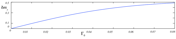
Figure S3: Magnetization oscillation amplitude at resonance as function of the spin-charge coupling parameter $\Gamma_{0}$.

References

- [1] T. Nozaki, Y. Shiota, S. Miwa, S. Murakami, F. Bonell, S. Ishibashi, H. Kubota, K. Yakushiji, T. Saruya, A. Fukushima, S. Yuasa, T. Shinjo and Y. Suzuki, Electric-field-induced ferromagnetic resonance excitation in an ultrathin ferromagnetic metal layer. Nat. Phys. 8, 491 (2012).
- [2] Y. Shiota, T. Maruyama, T. Nozaki, T. Shinjo, M. Shiraishi and Y. Suzuki, Voltage-Assisted Magnetization Switching in Ultrathin Fe80Co20 Alloy Layers. Appl. Phys. Express 2, 063001 (2009).
- [3] S. Kanai, M. Yamanouchi, S. Ikeda, Y. Nakatani, F. Matsukura, and H. Ohno, Electric field-induced magnetization reversal in a perpendicular-anisotropy CoFeB-MgO magnetic tunnel junction. Appl. Phys. Lett. 101, 122403 (2012).
- [4] J. Zhu, J.A. Katine, G.E. Rowlands, Y.J. Chen, Z. Duan, J.G. Alzate, P. Upadhyaya, J. Langer, P.K. Amiri, K.L. Wang, I.N. Krivorotov, Voltage-Induced Ferromagnetic Resonance in Magnetic Tunnel Junctions. Phys. Rev. Lett. 108, 197203 (2012).
- [5] Y. Suzuki, H. Kubota, A. Tulapurkar, and T. Nozaki, Spin control by application of electric current and voltage in FeCoMgO junctions. Phil. Trans. R. Soc. A 369, 3658 (2011).
- [6] D. Chiba, M. Sawicki, Y. Nishitani, Y. Nakatani, F. Matsukura, and H. Ohno, Magnetization vector manipulation by electric fields. Nat. Lett. 455, 515 (2008).
- [7] L. Gerhard, T. K. Yamada, T. Balashov, A. F. Takács, R. J. H. Wesselink, M. Däne, M. Fechner, S. Ostanin, A. Ernst, I. Mertig, and W. Wulfhekel, Magnetoelectric coupling at metal surfaces. Nat. Nano. 5, 792 (2010).
- [8] Y. Yamada, K. Ueno, T. Fukumura, H. T. Yuan, H. Shimotani, Y. Iwasa, L. Gu, S. Tsukimoto, Y. Ikuhara, and M. Kawasaki, Electrically Induced Ferromagnetism at Room Temperature in Cobalt-Doped Titanium Dioxide. Science 332, 1065 (2011).
- [9] E. Rashba, Properties of semiconductors with an extremum loop. 1. Cyclotron and combinational resonance in a magnetic field perpendicular to the plane of the loop. Sov. Phys. Solid State 2, 1109 (1960).
- [10] A. Manchon, H. C. Koo, J. Nitta, S. M. Frolov and R. A. Duine, New perspectives for Rashba spin-orbit coupling. Nat. Mat. 14, 871 (2015).
- [11] I. E. Dzyaloshinskii, Thermodynamic theory of weak ferromagnetism in antiferromagnetic substances. Sov. Phys. JETP 5, 1259 (1957).
- [12] T. Moriya, Anisotropic superexchange interaction and weak ferromagnetism. Phys. Rev. 120, 91 (1960).
- [13] A. Sekine and T. Chiba, Electric-field-induced spin resonance in antiferromagnetic insulators: Inverse process of the dynamical chiral magnetic effect. Phys. Rev. B 93, 220403(R) (2016).
- [14] J. Jensen and A.R. Mackintosh, Rare Earth Magnetism, (Clarendon Press, 1991).
- [15] S. Blundell, Magnetism in Condensed Matter, (Oxford University Press, 2012).
- [16] R. Skomski, Simple Models of Magnetism, (Oxford University Press, 2008).
- [17] R. Skomski and J. M. D. Coey, Permanent Magnetism, (Institute of Physics Publishing, 1999).
- [18] R. Skomski and D.J. Sellmyer, Anisotropy of rare-earth magnets,. J. Rare Earth 27, 675 (2009).
- [19] C. Tang, P. Sellappan, Y. Liu, Y. Xu, J.E. Garay, and J. Shi, Anomalous Hall hysteresis in Tm3Fe5O12/Pt with strain-induced perpendicular magnetic anisotropy. Phys. Rev. B 94, 140403(R) (2016).
- [20] As a consequence of strong electric fields, the electron polarize (Stark effect). This is a bulk effect. Furthermore, the energy of the Stark effect scales [5] as , and then this is a much smaller effect, that we disregard here.
- [21] Y. Shiota, S. Murakami, F. Bonell, T. Nozaki, T. Shinjo and Y. Suzuki, Quantitative Evaluation of Voltage-Induced Magnetic Anisotropy Change by Magnetoresistance Measurement. Appl. Phys. Express 4, 043005 (2011).
- [22] M. Tsujikawa,S. Haraguchi, and T. Oda, Effect of atomic monolayer insertions on electric-field-induced rotation of magnetic easy axis. J. Appl. Phys. 111, 083910 (2012).
- [23] A.A. Baker, A.I. Figueroa, G. van der Laan, T. Hesjedal, Tailoring of magnetic properties of ultrathin epitaxial Fe films by Dy doping. AIP ADVANCES 5, 077117 (2015).
- [24] W. Zhang, D. Zhang, P.K.J. Wong, H. Yuan, S. Jiang, G. van der Laan, Y. Zhai, and Z. Lu, Selective Tuning of Gilbert Damping in Spin-Valve Trilayer by Insertion of rare earth Nanolayers. ACS Appl. Mater. Interfaces 7, 17070 (2015).
- [25] See Supplemental Material at - for different derivations of the voltage coupling energy and torque. The results are equivalent. This material also shows the details of the numerical integration of the magnetization dynamics.
- [26] N.W. Ashcroft, N.D. Mermin, Solid State Physics (Brooks/Cole, Belmont, 1976).
- [27] R. Metselaar and P. K. Larsen, High-temperature electrical properties of yttrium iron garnet under varying oxygen pressures. Solid State Commun. 15, 291 (1974).
- [28] H. Pascard. Fast-neutron-induced transformation of the Y3Fe5O12 ionic structure. Phys. Rev. B 30, 2299(R) (1984).
- [29] R. Verba, V. Tiberkevich, I. Krivorotov, and A. Slavin, Parametric Excitation of Spin Waves by Voltage-Controlled Magnetic Anisotropy. Phys. Rev. Appl. 1, 044006 (2014).
- [30] C. Song, B. Cui, F. Li, X. Zhou, F. Pan, Recent progress in voltage control of magnetism: Materials, mechanisms, and performance. Progr. in Mat. Sc. 87, 33 (2017).

References

- [1] S. Zhang, Spin-Dependent Surface Screening in Ferromagnets and Magnetic Tunnel Junctions. Phys. Rev. Lett. 83, 640 (1999).
- [2] W. H. Press, S. A. Teukolsky, W. T. Vetterling, and B. P. Flannery, Numerical recipes in C: the art of scientific computing, (Cambridge University Press, New York, 1992)