MLSEB: Edge Bundling using Moving Least Squares Approximation

Abstract

Edge bundling methods can effectively alleviate visual clutter and reveal high-level graph structures in large graph visualization. Researchers have devoted significant efforts to improve edge bundling according to different metrics. As the edge bundling family evolve rapidly, the quality of edge bundles receives increasing attention in the literature accordingly. In this paper, we present MLSEB, a novel method to generate edge bundles based on moving least squares (MLS) approximation. In comparison with previous edge bundling methods, we argue that our MLSEB approach can generate better results based on a quantitative metric of quality, and also ensure scalability and the efficiency for visualizing large graphs.

1 Introduction

Traditional exploration methods of large graphs are often overwhelmed by severe visual clutter such as excessive vertex overlappings and edge crossings. Edge bundling is one of the effective approaches to reducing edge crossings in graph drawings. The main idea of edge bundling is to visually merge edges with similar features (e.g., position, direction, and length) such that edge crossings are significantly reduced and the readability of graph drawings is improved.

Substantial efforts have been made to develop various edge bundling algorithms to improve visual results. The current edge bundling family have provided a diverse graph layouts that work with a wide spectrum of applications and domains based on different strategies or metrics [22]. As the edge bundling techniques develop rapidly, the information visualization community is putting increasing interests in evaluating the results of edge bundle drawings. The readability and faithfulness criteria are often used to evaluate graph drawings. Edge bundling helps simplify graph drawings and increase readability, but yields distortion that makes it hard to preserve the faithfulness of original graphs [32]. To holistically address the evaluation of both readability and faithfulness for edge bundling visualization, Lhuillier et al. [22] suggested a general metric where a ratio of clutter reduction to amount of distortion is computed to measure the quality of edge bundling visualization. In this work, we aim to generate high-quality edge bundling results based on Lhuillier’s suggestion, and meanwhile ensure scalability and efficiency.

We introduce a novel edge bundling technique to generate edge bundles with moving least squares (MLS) approximation, namely MLSEB. Inspired by thinning an unorganized point cloud to curve-like shapes [20], we use a distance-minimizing approximation function to generate bundle effects. In particular, we first sample a graph into a point cloud data, and then use a moving least squares projection to generate curve-like bundles. Based on Lhuillier’s suggestion, we develop a quality assessment to evaluate edge bundling results. Using different real-world datasets, we demonstrate that MLSEB can produce bundle results with a higher quality, and is scalable and efficient for large graphs by comparing different edge bundling methods.

2 Related Work

The recent study [22] has surveyed the state-of-the-art edge bundling techniques and their applications in a very detailed manner. We revisit some of these methods by briefly summarizing the categories of the diverse bundling techniques. We consider our method as an image-based method, and hence we will discuss the image-based methods in more details. We will also cover some studies of quality evaluation in edge bundling and some studies on moving least squares approximation.

Holten [11] pioneered the edge bundling techniques in graph drawings using a hierarchical structure. Geometric-based methods [4, 17, 18, 25] used a control mesh to guide bundling process. Energy-based minimization methods have been also used in many studies. Examples include ink-minimization methods [8, 9] and force-directed methods [12, 31, 38, 44, 45]. Most of these methods used compatibility criteria to measure the similarity of different edges based on spatial information (i.e., length, position, angle, and visibility), and then moved the similar edges with ink-minimization or force-directed strategies.

Image-based techniques used a density assessment to guide bundling process [3, 6, 13, 23, 34, 46]. These methods are generally based on Kernel Density Estimation. Kernel density estimation edge bundling (KDEEB) [13] first transformed an input graph into a density map using kernel density estimation, and then moved the sample points of edges towards the local density maxima to form bundles. Peysakhovich et al. [34] extended KDEEB using edge attributes to distinguish bundles. CUDA Universal Bundling (CUBu) [46] used GPU acceleration to enable interactively bundling a graph with a million edges. Fast Fourier Transform Edge Bundling (FFTEB) [23] improved the scalability of density estimation by transforming the density space to the frequency space.

There are other edge bundling studies. Bach et al. [2] investigated the connectivity of edge bundling methods on Confluent Drawings. Nguyen et al. [30] proposed an edge bundling method for streaming graphs, which extended the idea of TGI-EB [31]. Wu et al. [43] used textures to accelerate bundling for web-based applications. Kwon et al. [16] showed their layout, rendering, and interaction methods for edge bundling in an immersive environment.

Serval studies introduced general metrics to quantify the readability [5, 36, 37, 39] and the faithfulness [29] of graph drawings. Some existing studies in edge bundling have defined quality assessments to evaluate the resulting bundles. Nguyen et al. [32] conducted a study on the faithfulness for force-directed edge bundling methods. Telea et al. [40] posed a comparison between different hierarchical edge bundling methods. Telea et al. [41] surveyed the hierarchical edge bundling techniques and posed a comparison of the quality of bundled and unbundled graphs. Pupyrev et al. [35] and Kobourov et al. [15] worked towards measuring edge crossings. KDEEB [13] and CUBu [46] proposed post-relaxation if the distortion of edge bundles is too large, such that the mental map is preserved. For sequence graph edge bundling, Hurter et al. [14] used interpolation to preserve the mental map between sequence graphs. McGee et al. [26] conducted an empirical study on the impact of edge bundling.

Moving least squares (MLS) has been widely used to approximate smooth curves and surface from unorganized point clouds [1, 21, 27]. Lee [20] constructed a curve-like shape from unorganized point clouds using an Euclidean minimum spanning tree. Least square projection (LSP) has been used in graph drawings [33], where multidimensional data points are projected into lower dimensions, while the similar relationship in neighboring points is preserved.

3 Background

3.1 Definition of Edge Bundling

We first revisit a formal definition of edge bundling [23]. Let $G=(V,E)\subset\mathbb{R}^{2},V=\{v_{i}\},E=\{e_{i}\}$ be a graph, where $v_{i}$ is a vertex and $e_{i}$ is an edge of $G$. Let $D:E\rightarrow\mathbb{R}^{2}$ be a drawing operator, such that $D(G)$ represents the drawing of $G$ and $D(e_{i})$ represents the drawing of an edge $e_{i}$. We define a compatibility operator $\phi$, where $\phi(e_{i},e_{j})$ measures the similarity of two edges $e_{i}$ and $e_{j}$. Edges that are more similar than a threshold $\phi_{max}$ should be bundled together, and $\phi$ can be used with some reasonable attributes and metrics(e.g., spatial information [12]). Let $B:\mathcal{D}\rightarrow\mathcal{D}$ be a bundling operation, where $\mathcal{D}\subset\mathbb{R}^{2}$ denotes the space of all graph drawings, and $B(D(e_{i}))$ denotes the resulting bundled drawing of $e_{i}$. For example, $D(e_{i})$ can be a straight line drawing and $B(D(e_{i}))$ can be a drawing of curve or polyline. Hence, an edge bundling algorithm can be expressed as:

$$\begin{split}&\forall(e_{i}\in G,e_{j}\in G)|\phi(e_{i},e_{j})<\phi_{max}\rightarrow\\ &\delta(B(D(e_{i})),B(D(e_{j})))\ll\delta(D(e_{i}),D(e_{j})),\end{split}$$ (1)

where $\delta$ is a distance metric in $\mathbb{R}^{2}$. Different edge bundling approaches explored various $\phi$, $B$, and $\delta$ to tackle Equation 1 to gain different visual effects of edge bundling [22].

3.2 Quality of Edge Bundling

Edge bundling techniques trade the increase of readability for overdrawing by bending edges to form bundle effects. Hence, edge bundle techniques naturally generate distortion from original graphs. To quantify the quality of a bundled graph, Lhuillier et al. [22] suggested to use the ratio of clutter reduction $C$ to amount of distortion $T$ as a quality metric $Q$, i.e.,

$${Q=\frac{C}{T}},$$ (2)

In general, a larger $Q$ corresponds to a higher quality, and vice versa. Lhuillier et al. [22] further posed a distortion measure. Simply, for an edge $e_{i}$, the distortion between an unbundled drawing $D(e_{i})$ and a bundled result $B(D(e_{i}))$ is measured by computing the distance between them, i.e., $\delta(D(e_{i}),B(D(e_{i})))$. Therefore, the overall distortion $T$ between an original unbundled graph and its bundled result can be defined as:

$${T=\sum_{i=1}^{n}\delta(D(e_{i}),B(D(e_{i})))},$$ (3)

where $n$ is the number of edges. Equation 3 provides an intuitive metric to evaluate the distortion generated by a bundled graph. The calculation of clutter reduction has not been fully concluded in the existing work. We propose a simple method to evaluate clutter reduction $C$, modify Equation 3 to compute $T$, and then use $C$ and $T$ to quantify the quality $Q$ of edge bundling (Section 6.2).

4 Our Bundling Algorithm

The main purpose of edge bundling is to achieve appealing bundle effects by bending edges, expressed by Equation 1. Meanwhile, according to Equation 2, an ideal algorithm should increase clutter reduction $C$, while decrease amount of distortion $T$, in order to achieve a higher quality $Q$ of edge bundling. Therefore, we should holistically address Equations 1 and 2, which, however, has not been fully investigated in the existing work [22].

4.1 Sampling

In general, given a graph $G$, a polyline is used to draw the line or curve presentation of an edge $e_{i}$. Sample points $x^{i}_{k}$, namely sites, are used to discretize the drawing of $e_{i}$. Formally,

$${\{x^{i}_{k}|1\leq k\leq m_{i}\}\approx D(e_{i})},$$ (4)

where $m_{i}$ is the number of sites for $D(e_{i})$. Note, many methods [13, 23, 34, 46] use a sampling step that is a small fraction of the size of the display to sample each edge, which means the number of sites of $D(e_{i})$ may be different. Similarly, the bundled drawing can also be discretized as:

$${B(\{x^{i}_{k}|1\leq k\leq m_{i}\})\approx B(D(e_{i}))}.$$ (5)

We measure the distortion between $D(e_{i})$ and $B(D(e_{i}))$ by summing the Euclidean distance between each pair of $x^{i}_{k}$ and $B(x^{i}_{k})$. Let $|\cdot|$ denote the Euclidean distance. Replace the edges in Equation 3 using Equation 4 and Equation 5, we have

$${T=\sum_{i=1}^{n}(\sum_{k=1}^{m_{i}}|\{x^{i}_{k}\},B(\{x^{i}_{k}\})|}).$$ (6)

Similarly, Equation 1 can be modified as:

$$\begin{split}&\forall(e_{i}\in G,e_{j}\in G)|\phi(e_{i},e_{j})<\phi_{max}\rightarrow\\ &|B(\{x^{i}_{k}\}),B(\{x^{j}_{k}\})|\ll|\{x^{i}_{k}\},\{x^{j}_{k}\}|.\end{split}$$ (7)

Therefore, we discretize each edge drawing $D(e_{i})$ of $G$ by Equation 4. All the sample points generated by Equation 4 form a point cloud. According to Equation LABEL:eq:equation_3, $x^{i}_{k}$ is moved to a new position $B(x^{i}_{k})$ by a bundling operator B. In the case of kernel density estimation edge bundling [13, 23, 34, 46], $x^{i}_{k}$ is moved to $B(x^{i}_{k})$ according to its local density gradient. These methods form the bundles by gathering sample points to their local density maxima, but do not consider the distortion of edges when moving sample points. Therefore, certain artifacts, such as lattice effects and subsampled edge fragments, can be incurred. The methods, such as resampling and post-relaxation [13, 46], have been proposed to address these issues. However, these methods typically introduce a significant performance overhead that is challenging to alleviate [46]. We develop a new bundling operator $B$ with respect to Equation LABEL:eq:equation_3, and minimize the distortion of each sample point locally. Moreover, our method does not require resampling, and thereby can reduce the computational cost.

4.2 Moving Least Squares Approximation

We consider all the points formed by sampling, and assess the global distortion by expressing Equation 6 as:

$$\mathcal{T}=\sum_{i=1}^{S}{|x_{i}-B(x_{i})|^{2}},$$ (8)

where $x_{i}$ is a site in the point cloud, and $S$ is the number of sites of all edges.

We assume there is a skeleton near $x_{i}$ and its neighborhood locally. A skeleton can be a suitable place to gather curves to form bundles [6]. Assume a skeleton can be interpreted as an implicit polynomial or piece-wise polynomial curve $f_{i}$, which is unknown. The unknown $f_{i}$ can be gained by computing the coefficients of $f_{i}$, i.e., by minimizing the following weighted least squares error $\epsilon$ within a set $\mathcal{H}(x_{i})$ consisting of $x_{i}$ and its neighbor sites:

$$\epsilon=\sum_{j=1}^{h_{i}}{|x_{j}-f_{i}|^{2}\theta(|x_{j}-x_{i}|)},$$ (9)

where $x_{i}\in\mathcal{H}(x_{i})$, $x_{j}\in\mathcal{H}(x_{i})$, $h_{i}$ is the size of $\mathcal{H}(x_{i})$, and $|x_{j}-f_{i}|$ means the shortest Euclidean distance between $x_{j}$ and $f_{i}$. We define the bundling operator $B$ on $x_{i}$ as a two-step procedure: first to construct $f_{i}$, and then to project $x_{i}$ onto $f_{i}$. The projected point is thereby $B(x_{i})$ that is on $f_{i}$. The distance $|x_{i}-B(x_{i})|$ from $x_{i}$ to $B(x_{i})$ is locally minimized by an appropriate nonnegative weighting function $\theta$. The input of $\theta$ is $|x_{j}-x_{i}|$, which is the distance of neighborhood $x_{j}$ to the site $x_{i}$. Instead of taking all sites of a graph into account, we use a circle of radius $r$ (bandwidth) centered at $x_{i}$ to collect the neighborhood $x_{j}$ for $x_{i}$.

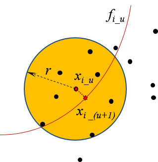
Figure 1: Two steps of our bundling operator $B$ on a site $x_{i\_u}$ in an iteration $u$. First, a local implicit regression curve $f_{i\_u}$ is constructed by the neighborhood of $x_{i\_u}$ with a bandwidth $r$ using the MLS approximation. Second, $x_{i\_u}$ is moved to a new position $x_{i\_(u+1)}$ that is the projection of $x_{i\_u}$ on $f_{i\_u}$.

If $\theta\equiv 1$, a least squares (LS) approximation is generated. However, LS approximation does not work well to generate a polynomial curve that locally reflects the density distribution of neighborhood. Alternatively, the moving least squares (MLS) method can reduce a point cloud to a thin curve-like shape that is a near-best approximation of the point set [20, 21]. Hence, we use a local assessment to approximate $f_{i}$ [19]. The weighting function we use is a cubic function [27]:

$$\theta(d)=\begin{dcases*}2\frac{d^{3}}{r^{3}}-3\frac{d^{2}}{r^{2}}+1&if $d<r$,\\[12.91663pt] 0&if $d\geq r$,\end{dcases*}$$ (10)

where $d=|x_{j}-x_{i}|$. In this sense, minimizing Equation 9 leads to an MLS approximation so that $f_{i}$ is a local regression curve, and $|x_{i}-B(x_{i})|$ is locally minimized. In other words, the distortion is locally minimized.

In our work, we use an MLS approximation to evaluate the distance $|x_{j}-f_{i}|$ for the neighborhood $\mathcal{H}(x_{i})$ of $x_{i}$. Therefore, we use a basic projection [19] to construct the implicit local regression curve $f_{i}$: We take a partial derivative of Equation 9 with respect to each coefficient of $f_{i}$, make each partial derivative equal to zero, and then solve the system of equations to generate all the coefficients of $f_{i}$ [28].

Similar to existing work [6, 13, 23, 34, 46], we implement our bundling operator $B$ through an iteration strategy. In our method, two steps are applied iteratively, as shown in Figure 1. We initially treat $x_{i}$ as $x_{i\_0}$. Then, in each iteration $u$, the first step is to construct an optimal regression curve $f_{i\_u}$ by thinning the unordered point cloud within $\mathcal{H}(x_{i\_u})$, the neighborhood of $x_{i\_u}$. In the second step, we project $x_{i\_u}$ onto $f_{i\_u}$ and obtain the projected point $x_{i\_(u+1)}$, i.e., $B(x_{i\_u})$. In this way, a site $x_{i\_u}$ is moved to $x_{i\_(u+1)}$ based on the weighting function $\theta$ of its neighborhood $\mathcal{H}(x_{i\_u})$. Different from the kernel density estimation methods [6, 13, 23, 34, 46], MLS moves the site $x_{i\_u}$ in the sense that the local error $\epsilon$ is bounded with the error of a local best polynomial approximation [20]. In our current work, this process stops when the iteration number reaches a predefined threshold. Then, for each edge, we compute a B-spline curve based on the final positions of its sites. Figure 2 shows an example with two different iterations. For an illustration purpose, we show the corresponding B-spline curves for the iterations. In Figure 2, we can see that a curve-like skeleton is gradually formed from the point cloud through the iterations in the top row, and a bundle effect becomes increasingly distinct as shown by the B-spline results in the bottom row.

$\begin{array}[]{c@{\hspace{0.01\linewidth}}c@{\hspace{0.01\linewidth}}c}\includegraphics[width=143.09538pt]{sample_0_small}\hfil\hskip 4.33382pt&\includegraphics[width=143.09538pt]{sample_2_small}\hfil\hskip 4.33382pt&\includegraphics[width=143.09538pt]{sample_10_small}\\ \includegraphics[width=143.09538pt]{sample_0_curve_small}\hfil\hskip 4.33382pt&\includegraphics[width=143.09538pt]{sample_2_curve_small}\hfil\hskip 4.33382pt&\includegraphics[width=143.09538pt]{sample_10_curve_small}\\ \mbox{\scriptsize{Iteration 0}}\hfil\hskip 4.33382pt&\mbox{\scriptsize{Iteration 2}}\hfil\hskip 4.33382pt&\mbox{\scriptsize{Iteration 8}}\end{array}$

Figure 2: Using an US airlines dataset as an example, we first sample each edge into a set of points (or sites). The resulting sites form a point cloud (top-left). The top row shows the point cloud is converged through an iterative MLS processing. The bottom row shows the corresponding B-spline results. The first column shows the initial result before MLS. The following columns show the results generated after the 2nd and 8th iteration, respectively.

Most of the existing image-based techniques use kernel density estimation (KDE), essentially, a mean-shift method that evaluates the local density maxima and advects a site based on the gradients of the local density. However, KDE does not consider the distortion (Equation 3) when moving sample points, and thus resampling or post-relaxation is often required [13, 46]. Alternatively, our MLSEB method uses an MLS approximation that projects a site $x_{i}$ to its local regression curve $f_{i}$, where $f_{i}$ is locally approximated by minimizing the distance between $\mathcal{H}(x_{i})$ and $f_{i}$ with a weighted function (Equation 9). Therefore, the distance between its original position $x_{i}$ and its projected position $B(x_{i})$ is locally minimized based on the density of its neighborhood $\mathcal{H}(x_{i})$. One advantage of our method is that MLS does not need to resample each edge in bundling iterations because sites are projected into curves that do not generate over-converge artifacts or lattice effects. Fröhlich et al. [7] showed that MLS produced better convergence results than KDE in biological studies. However, it remains an open question to determine if KDE or MLS is better than one another in edge bundling. In Section 6.2, we will develop a quality assessment from Equation 2, and use it to evaluate and compare the quality of the drawings generated by our MLSEB method, the FFTEB method (a KDE-based method), and the FDEB method (a force-directed method).

5 Implementation

Our implementation involves simple data structures and computations, and thus is easy to implement. First, we sample the edges of an input graph. We use the same scheme as KDEEB’s [13] to sample the input edges with an uniform step $\rho$. The most time consuming step in our method is gathering the neighborhood for every site. A typical solution in a GPU implementation is to use Uniform Grid [10] that subdivides the space into uniformly sized cells. We use this method and set the size of the cell to be $\frac{2}{3}r$ ($r$ is a prescribed radius or bandwidth) such that we can limit the search space of each site to only cover at most 9 grid cells [10], thus avoid a $O(S^{2})$ search time for $S$ sites.

At the start of each iteration, all the sites are put into the corresponding cells according to their current positions. This can be easily parallelized using CUDA on a GPU [10]. Then, we project each site onto its local regression line. The solution to compute the coefficients of Equation 9 is introduced in the work [19, 28]. It only requires a constant time to solve the coefficients of a linear or quadratic system of equations. This can also be parallelized using a GPU because computing the new projection position for every site is independent.

To enhance the visualization of a bundled graph, we use the same shader scheme of CUBu [46]. We use the HSVA (i.e., hue $H$, saturation $S$, value $V$, and alpha $A$) color representation to visualize edges. Each edge site $x_{i}$ is encoded with an HSVA value. We encode the direction and the length of the corresponding edge into $H$ and $S$, respectively. $V$ and $A$ are used with a parabolic profile function $c(x)=\sqrt{1-2|t(x)-\frac{1}{2}|}$, and $t\in[0,1]$ is the edge arc-length parameterization. The functions of $V$ and $A$ are then $V(x)=\frac{l}{l_{max}}+(1-\frac{l}{l_{max}})c(x)$ and $A(x)=\alpha(1-\frac{l}{l_{max}}+\frac{l}{l_{max}}c(x))$ respectively, where $l$ is the length of the edge, $l_{max}$ is the longest edge in the graph, and $\alpha$ controls the overall transparency of all edges.

Next, we analyze the complexity of our MLSEB method. Similar to the existing KDE-based methods [13, 23, 34, 46], MLSEB requires gathering neighbor sites for computation. After gathering, KDE-based methods conduct kernel splatting, gradient calculation, and site advection, which use a constant time for each site. In MLSEB, the time to solve Equation 9 and project a site to its local approximated curve is also constant for each site. Thereby, the complexity of MLSEB is the same as the traditional KDE-based methods, which is $O(I\cdot N\cdot S)$, where $I$ is the image resolution, $N$ is the number of bundling iterations, and $S$ is the number of sample points. However, MLSEB does not need additional operations, such as resampling, that are employed in the existing KDE-based methods.

We explore the parameter choices of MSLEB as follows. Similar to most the existing edge bundling methods, we use a step $\rho$, which is $5\%$ of the image resolution $I$, to sample each edge. The bandwidth, $r$, plays an important role in MLS to estimate the density information around each site. A larger bandwidth captures more sample sites to reflect a more global feature, while a smaller bandwidth reveals a more local feature. By following a similar strategy in FDEB [45] and KDEEB [13], we decrease $r$ by a reduction factor $\lambda$ after each iteration. Hurter et al. [13] stated that a kernel size follows an average density estimation when $0.5\leq\lambda\leq 0.9$. We set $r$ to be $5\%\leq r\leq 20\%$ of the display size $I$ to generate a stable edge-convergence result. Through a heuristic study, we found that it is sufficient to yield good results by setting the iteration number $N$ between 3 and 10 and making the polynomial order of $f_{i}$ in Equation 9 to be 1 or 2.

6 Results

6.1 Visualization and Performance Results

$\begin{array}[]{c@{\hspace{0.01\linewidth}}c}\includegraphics[width=212.47617pt]{airline_1_small}\hfil\hskip 4.33382pt&\includegraphics[width=212.47617pt]{migration_2_small}\\ \mbox{\scriptsize{(a)}}\hfil\hskip 4.33382pt&\mbox{\scriptsize{(b)}}\end{array}$

Original Node-link Diagrams

$\begin{array}[]{c@{\hspace{0.01\linewidth}}c}\includegraphics[width=212.47617pt]{compare_airline_fdeb_small}\hfil\hskip 4.33382pt&\includegraphics[width=212.47617pt]{compare_migration_fdeb_small}\\ \mbox{\scriptsize{(c)}}\hfil\hskip 4.33382pt&\mbox{\scriptsize{(d)}}\end{array}$

FDEB

$\begin{array}[]{c@{\hspace{0.01\linewidth}}c}\includegraphics[width=212.47617pt]{compare_airline_ffteb_small}\hfil\hskip 4.33382pt&\includegraphics[width=212.47617pt]{compare_migration_ffteb_small}\\ \mbox{\scriptsize{(e)}}\hfil\hskip 4.33382pt&\mbox{\scriptsize{(f)}}\end{array}$

FFTEB

$\begin{array}[]{c@{\hspace{0.01\linewidth}}c}\includegraphics[width=212.47617pt]{result_airline}\hfil\hskip 4.33382pt&\includegraphics[width=212.47617pt]{result_migration}\\ \mbox{\scriptsize{(g)}}\hfil\hskip 4.33382pt&\mbox{\scriptsize{(h)}}\end{array}$

MLSEB

Figure 3: Visualize the US airlines dataset (the left column) and the US migrations dataset (the right column) with three different edge bundling methods, FDEB, FFTEB and MLSEB, respectively.

$\begin{array}[]{ccc}\includegraphics[width=143.09538pt]{result_FDEB_airline_small}&\includegraphics[width=143.09538pt]{compare_france_ffteb_small}&\includegraphics[width=143.09538pt]{result_france}\\ \mbox{\scriptsize{FDEB}}&\mbox{\scriptsize{FFTEB}}&\mbox{\scriptsize{MLSEB}}\end{array}$

Figure 4: Visualize the France airlines dataset (17274 edges) with FDEB, FFTEB, and MLSEB.

$\begin{array}[]{c@{\hspace{0.01\linewidth}}c}\includegraphics[width=212.47617pt]{largeMigration_FFTEB_small}\hfil\hskip 4.33382pt&\includegraphics[width=212.47617pt]{largeMigration_MLSEB_small}\\ \mbox{\scriptsize{FFTEB}}\hfil\hskip 4.33382pt&\mbox{\scriptsize{MLSEB}}\end{array}$

Figure 5: Comparison of FFTEB and MLSEB using a large US migrations dataset (545881 edges).

We apply our MLSEB method to several graphs and compare its effect and computational performance to the two existing methods: FDEB that is the classic force-directed method, and FFTEB that is the latest enhanced KDE-based method of image-based edge bundling algorithms (such as KDEEB and CUBu).

The left column in Figure 3 compares the visualization results of our MLSEB method with other bundling methods using the US airlines dataset (2101 edges). Our MLSEB method provides similar results, and generates tight, smooth and locally well-separated bundles. High-level graph structures are also revealed in our results. The right column in Figure 3 shows the comparison using the US migrations dataset (9780 edges). Figure 4 shows another example using the France airlines dataset with 17274 edges. In these results, the main migration and airline patterns are clearly revealed using MLSEB. In the migrations dataset, FDEB and FFTEB fall short in showing some subtle structures of the original graph. For example, in the original node-link diagram of Figure 3(b), the edges (within the red box) connect the city of Portland to some cities in the northern U.S are distorted significantly from their original positions in the results of the FDEB (Figure 3(d)) and FFTEB (Figure 3(f)), while our MLSEB result has a distinguished bundle effect that reveals this subtle graph structure. In Figure 5, we compare the visual result of MLSEB to FFTEB using a large US migrations dataset with 545881 edges. We encode the color of a edge with only its length in this example. MLSEB shows more long-length edge patterns than FFTEB.

Table 1 shows the performance comparison between our MLSEB method and the current fastest edge bundling method FFTEB. In our performance comparison, we used the US airlines graph, the US migrations graph, the France airlines graph, and the large US migrations graph. The timing results for MLSEB and FFTEB are based on one iteration, and we excluded the timing of memory allocation and data transferring for both methods. The devices used in our experiments are a desktop with an 8X Intel Core i7-6700K 4.0GHz CPU with 32GB memory and a NVIDIA GeForce GTX TITAN X GPU. Comparing with the fastest algorithm FFTEB in the state-of-the-art, we can clearly see that MLSEB is at the same order of magnitude of FFTEB in terms of computational speed, as shown in Table 1.

Table 1: Performance comparison.

Graph	Edges	FFTEB		MLSEB
		Samples	Time (ms)	Samples	Time (ms)
US airlines	2180	105K	40	85K	22
US migrations	9780	489K	48	207K	38
France airlines	17274	864K	70	990K	94
Large US migrations	545881	6.4M	123	5.8M	554

6.2 Quality Assessment of Bundled Graphs

Apart from comparing the visualization and performance results, we propose a quality metric to evaluate the quality of bundling drawings based on Equation 2.

Equation 2 gives a general quality metric $Q$ based on the ratio of clutter reduction $C$ to amount of distortion $T$. However, the quantification of clutter reduction $C$ has been not fully concluded in existing work. We propose to employ the reduction of the used pixel number $\Delta{P}$ in a graph drawing to measure $C$. Specifically, $C=\Delta{P}=P-P^{\prime}$ that is the difference of the used pixel number $P$ of the original drawing and the used pixel number $P^{\prime}$ of the bundled drawing.

Intuitively, $T$ can be given by Equation 6 that quantifies the total distortion of all the sample points. However, different methods can generate different numbers of sample points. For example, FDEB generates the same number of sample points for each edge, while our MLSEB method and the KDE-based methods sample different edges into different numbers of points. Thus, instead of the total distortion of all the sample points, we use the average distortion: $\overline{T}=\frac{T}{S}$, where $S$ is the total number of the sample points in the graph. Therefore, we modify Equation 2 to

$$Q=\frac{\Delta{P}}{\overline{T}}.$$ (11)

The rationale of Equation 11 is to measure how many pixels are decreased by generating one unit distortion. A higher value of $Q$ means a better quality result. Table 2 shows the quantitative quality comparison between our MLSEB method, FDEB and FFTEB. Our comparison is based on the drawings with an image resolution of $400\times 400$, as shown in Figures 3, 4, and 5. All the statistic results are generated after a graph is bundled, i.e., after all iterations. We note that it makes less sense to compare the distortion in each iteration because the initial iterations of some methods, such as FDEB and FFTEB, may have surprisingly large distortion. It is more reasonable to compare the quality of results after the bundling iterations are finished. We also note that using different parameters, such as different iteration numbers and different bandwidths for different methods, can yield different results. We use the recommended parameters in FDEB’s and FFTEB’s papers [12, 23], which are the best results we can get from the existing work. The $S$ columns in Table 2 show the numbers of the sample points in a graph using different methods.

Table 2: Quality comparison using the US migrations graph.

Graph	Edges	FDEB					FFTEB					MLSEB
		$S$	$P$	$P^{\prime}$	$\overline{T}$	$Q$	$S$	$P$	$P^{\prime}$	$\overline{T}$	$Q$	$S$	$P$	$P^{\prime}$	$\overline{T}$	$Q$
US airlines	2180	813K	32K	25K	1.10K	6.2	105K	32K	18K	1.2K	11.9	85K	32K	19K	0.88K	14.4
US migrations	9780	3785K	34K	26K	0.88K	8.9	489K	32K	24K	1.0K	7.60	207k	33k	25k	0.92k	9.20
France airlines	17274	6685K	81K	72K	2.60K	3.7	864K	81K	57K	1.6K	21.3	990K	81K	60K	0.80K	26.0
Large US migrations	545881	n/a	n/a	n/a	n/a	n/a	6.4M	108k	84k	1.8k	13.3	5.8M	107k	95k	0.90	13.3

We can see that the quality of MLSEB is generally better than the other two methods in terms of Equation 11. For the four different datasets, FFTEB makes the most clutter reduction. However, it also incurs more distortion. FDEB achieves a comparable quality as ours for the US migrations dataset; whereas, when the dataset is getting larger (France airlines), FDEB will generate tremendous distortion, as shown in Table 2 and Figure 4, thus lowering the quality score. Note when using the large US migrations dataset, the advantage of MLSEB over FFTEB becomes marginal. Overall, MLSEB gains the highest quantitative scores in terms of quality according to Equation 11.

7 Conclusions and Future Work

We present a new edge bundling method MLSEB that holistically considers distortion minimization and clutter reduction. Inspired by the MLS work [1, 20], our approach generate bundle effects by iteratively projecting each site to its local regression curve to converge with other nearby sites based on its neighborhood’s density. Such a local regression curve can reduce the distortion of the local bundle. Our method is easy to implement. The timing result shows MLSEB is at the same order of magnitude of the current fastest edge bundling method FFTEB in terms of computational speed.

We use a quality assessment to evaluate the quality of resulting edge bundles. Our MLSEB method shows better results in our preliminary comparison. However, a more comprehensive comparison between our MLSEB method and the other methods requires further investigation, where other factors (e.g., edge crossing reduction) may be also considered. In addition, we plan to apply optimal bandwidth selection [24, 42] to improve MLSEB. We would also like to incorporate semantic attributes into MLSEB to enhance bundling results. Last but not least, bundling a very large graph (e.g., one with billions or trillions of edges) remains a very challenging task, which is a next possible direction in our future work.

References

- [1] Alexa, M., Behr, J., Cohen-Or, D., Fleishman, S., Levin, D., T. Silva, C.: Computing and rendering point set surfaces. IEEE Transactions on Visualization and Computer Graphics 9(1), 3–15 (jan 2003)
- [2] Bach, B., Riche, N.H., Hurter, C., Marriott, K., Dwyer, T.: Towards unambiguous edge bundling: Investigating confluent drawings for network visualization. IEEE Transactions on Visualization and Computer Graphics 23(1), 541–550 (Jan 2017)
- [3] Böttger, J., Schäfer, A., Lohmann, G., Villringer, A., Margulies, D.S.: Three-dimensional mean-shift edge bundling for the visualization of functional connectivity in the brain 20(3), 471–480 (2014)
- [4] Cui, W., Zhou, H., Qu, H., Wong, P.C., Li, X.: Geometry-based edge clustering for graph visualization. IEEE Transactions on Visualization and Computer Graphics 14(6), 1277–1284 (Nov 2008)
- [5] Di Battista, G.: Graph drawing : algorithms for the visualization of graphs. Prentice Hall, Upper Saddle River, N.J. (1999)
- [6] Ersoy, O., Hurter, C., Paulovich, F., Cantareiro, G., Telea, A.: Skeleton-based edge bundling for graph visualization. IEEE Transactions on Visualization and Computer Graphics 17(12), 2364–2373 (2011)
- [7] Fröhlich, F., Hross, S., Theis, F.J., Hasenauer, J.: Radial basis function approximations of bayesian parameter posterior densities for uncertainty analysis. In: International Conference on Computational Methods in Systems Biology. pp. 73–85. Springer (2014)
- [8] Gansner, E.R., Hu, Y., North, S., Scheidegger, C.: Multilevel agglomerative edge bundling for visualizing large graphs. In: 2011 IEEE Pacific Visualization Symposium. pp. 187–194 (March 2011)
- [9] Gansner, E.R., Koren, Y.: Improved circular layouts. In: Proceedings of the 14th International Conference on Graph Drawing. pp. 386–398. GD’06, Springer-Verlag, Berlin, Heidelberg (2007)
- [10] Green, S.: Particle simulation using cuda. NVIDIA whitepaper 6, 121–128 (2010)
- [11] Holten, D.: Hierarchical edge bundles: Visualization of adjacency relations in hierarchical data. IEEE Transactions on Visualization and Computer Graphics 12(5), 741–748 (2006)
- [12] Holten, D., Wijk, J.J.v.: Force-Directed Edge Bundling for Graph Visualization. Computer Graphics Forum (2009)
- [13] Hurter, C., Ersoy, O., Telea, A.: Graph bundling by kernel density estimation. Comput. Graph. Forum 31(3pt1), 865–874 (Jun 2012)
- [14] Hurter, C., Ersoy, O., Telea, A.: Smooth bundling of large streaming and sequence graphs. In: 2013 IEEE Pacific Visualization Symposium (PacificVis). pp. 41–48 (Feb 2013)
- [15] Kobourov, S.G., Pupyrev, S., Saket, B.: Are Crossings Important for Drawing Large Graphs?, pp. 234–245. Springer Berlin Heidelberg, Berlin, Heidelberg (2014)
- [16] Kwon, O.H., Muelder, C., Lee, K., Ma, K.L.: A study of layout, rendering, and interaction methods for immersive graph visualization. IEEE Transactions on Visualization and Computer Graphics 22(7), 1802–1815 (July 2016)
- [17] Lambert, A., Bourqui, R., Auber, D.: 3d edge bundling for geographical data visualization. In: 2010 14th International Conference Information Visualisation. pp. 329–335 (July 2010)
- [18] Lambert, A., Bourqui, R., Auber, D.: Winding roads: Routing edges into bundles. In: Proceedings of the 12th Eurographics / IEEE - VGTC Conference on Visualization. pp. 853–862. EuroVis’10, The Eurographs Association & John Wiley & Sons, Ltd., Chichester, UK (2010)
- [19] Lancaster, P., Salkauskas, K.: Surfaces Generated by Moving Least Squares Methods. Mathematics of Computation 37(155), 141–158 (1981)
- [20] Lee, I.K.: Curve reconstruction from unorganized points. Comput. Aided Geom. Des. 17(2), 161–177 (Feb 2000)
- [21] Levin, D.: Mesh-Independent Surface Interpolation, pp. 37–49. Springer Berlin Heidelberg, Berlin, Heidelberg (2004)
- [22] Lhuillier, A., Hurter, C., Telea, A.: State of the art in edge and trail bundling techniques. Comput. Graph. Forum 36(3), 619–645 (Jun 2017)
- [23] Lhuillier, A., Hurter, C., Telea, A.: FFTEB: Edge Bundling of Huge Graphs by the Fast Fourier Transform. In: PacificVis 2017, 10th IEEE Pacific Visualization Symposium. IEEE, Seoul, South Korea (Apr 2017)
- [24] Lipman, Y., Cohen-Or, D., Levin, D.: Error bounds and optimal neighborhoods for mls approximation. In: Proceedings of the Fourth Eurographics Symposium on Geometry Processing. pp. 71–80. SGP ’06, Eurographics Association, Aire-la-Ville, Switzerland, Switzerland (2006)
- [25] Luo, S.J., Liu, C.L., Chen, B.Y., Ma, K.L.: Ambiguity-free edge-bundling for interactive graph visualization. IEEE Transactions on Visualization and Computer Graphics 18(5), 810–821 (May 2012)
- [26] McGee, F., Dingliana, J.: An empirical study on the impact of edge bundling on user comprehension of graphs. In: Proceedings of the International Working Conference on Advanced Visual Interfaces. pp. 620–627. AVI ’12, ACM, New York, NY, USA (2012)
- [27] Mederos, B., Velho, L., Figueiredo, L.H.D.: Moving least squares multiresolution surface approximation. In: 16th Brazilian Symposium on Computer Graphics and Image Processing (SIBGRAPI 2003). pp. 19–26 (Oct 2003)
- [28] Nealen, A.: An As-Short-As-Possible Introduction to the Least Squares, Weighted Least Squares and Moving Least Squares Methods for Scattered Data Approximation and Interpolation (2004)
- [29] Nguyen, Q., Eades, P., Hong, S.H.: On the Faithfulness of Graph Visualizations, pp. 566–568. Springer Berlin Heidelberg, Berlin, Heidelberg (2013)
- [30] Nguyen, Q., Eades, P., Hong, S.H.: StreamEB: Stream edge bundling. In: Proceedings of the 20th International Conference on Graph Drawing. pp. 400–413. GD’12, Springer-Verlag, Berlin, Heidelberg (2013)
- [31] Nguyen, Q., Hong, S.H., Eades, P.: TGI-EB: A New Framework for Edge Bundling Integrating Topology, Geometry and Importance, pp. 123–135. Springer Berlin Heidelberg, Berlin, Heidelberg (2012)
- [32] Nguyen, Q.H., Eades, P., Hong, S.: Towards faithful graph visualizations. CoRR abs/1701.00921 (2017)
- [33] Paulovich, F.V., Nonato, L.G., Minghim, R., Levkowitz, H.: Least square projection: A fast high-precision multidimensional projection technique and its application to document mapping. IEEE Transactions on Visualization and Computer Graphics 14(3), 564–575 (May 2008)
- [34] Peysakhovich, V., Hurter, C., Telea, A.: Attribute-driven edge bundling for general graphs with applications in trail analysis. In: 2015 IEEE Pacific Visualization Symposium (PacificVis). pp. 39–46 (April 2015)
- [35] Pupyrev, S., Nachmanson, L., Kaufmann, M.: Improving Layered Graph Layouts with Edge Bundling, pp. 329–340. Springer Berlin Heidelberg, Berlin, Heidelberg (2011)
- [36] Purchase, H.: Which aesthetic has the greatest effect on human understanding?, pp. 248–261. Springer Berlin Heidelberg, Berlin, Heidelberg (1997)
- [37] Purchase, H.C., Cohen, R.F., James, M.: Validating graph drawing aesthetics, pp. 435–446. Springer Berlin Heidelberg, Berlin, Heidelberg (1996)
- [38] Selassie, D., Heller, B., Heer, J.: Divided edge bundling for directional network data. IEEE Transactions on Visualization and Computer Graphics 17(12), 2354–2363 (Dec 2011)
- [39] Tamassia, R.: Handbook of Graph Drawing and Visualization (Discrete Mathematics and Its Applications). Chapman & Hall/CRC (2007)
- [40] Telea, A., Ersoy, O., Hoogendorp, H., Reniers, D.: Comparison of node-link and hierarchical edge bundling layouts: A user study. In: Keim, D.A., Pras, A., Schönwälder, J., Wong, P.C. (eds.) Visualization and Monitoring of Network Traffic. No. 09211 in Dagstuhl Seminar Proceedings, Schloss Dagstuhl - Leibniz-Zentrum fuer Informatik, Germany, Dagstuhl, Germany (2009)
- [41] Telea, A., Ersoy, O., Hoogendorp, H., Reniers, D.: Comparison of node-link and hierarchical edge bundling layouts: A user study. In: Keim, D.A., Pras, A., Schönwälder, J., Wong, P.C. (eds.) Visualization and Monitoring of Network Traffic. No. 09211 in Dagstuhl Seminar Proceedings, Schloss Dagstuhl - Leibniz-Zentrum fuer Informatik, Germany, Dagstuhl, Germany (2009)
- [42] Wang, H., Scheidegger, C.E., Silva, C.T.: Bandwidth selection and reconstruction quality in point-based surfaces. IEEE Transactions on Visualization and Computer Graphics 15(4), 572–582 (July 2009)
- [43] Wu, J., Yu, L., Yu, H.: Texture-based edge bundling: A web-based approach for interactively visualizing large graphs. In: 2015 IEEE International Conference on Big Data (Big Data). pp. 2501–2508 (Oct 2015)
- [44] Zhou, H.: Visual Clustering in Parallel Coordinates and Graphs. Ph.D. thesis (2009), aAI3398258
- [45] Zielasko, D., Weyers, B., Hentschel, B., Kuhlen, T.W.: Interactive 3d force-directed edge bundling. In: Proceedings of the Eurographics / IEEE VGTC Conference on Visualization. pp. 51–60. EuroVis ’16, Eurographics Association, Goslar Germany, Germany (2016)
- [46] van der Zwan, M., Codreanu, V., Telea, A.: Cubu: Universal real-time bundling for large graphs. IEEE Transactions on Visualization and Computer Graphics 22(12), 2550–2563 (Dec 2016)