Phenomenological Analysis of an $\mathrm{E}_{6}$-inspired Seesaw Model

Abstract

We analyse the phenomenology of a model of neutrino masses inspired by unification into $\mathrm{E}_{6}$ in which the exotic neutrinos can be present at low scales. The model introduces vector-like isosinglet down-type quarks, vector-like isodoublet leptons, neutrino singlets and two $Z^{\prime}$ bosons. The seesaw mechanism can be achieved with exotic neutrino masses as low as $100\text{\,}\mathrm{GeV}$ and Yukawa couplings of order ${10}^{-3}$. We find that the lightest $Z^{\prime}$ boson mass is required to be above $2.8\text{\,}\mathrm{TeV}$, the exotic quark masses are required to be above $1.3\text{\,}\mathrm{TeV}$ ($810\text{\,}\mathrm{GeV}$) if they are collider stable (promptly decaying), and the exotic lepton mass bounds remain at the lep value of $102\text{\,}\mathrm{GeV}$. The model also presents a type-ii two-Higgs-doublet model (2hdm) along with two heavy singlet scalars. The 2hdm naturally has the alignment limit enforced thanks to the large vacuum expectation values of the exotic scalars, thereby avoiding most constraints.

I Introduction

The origin of neutrino masses and their unusually small values in comparison to the other fermions of the Standard Model (sm) are still mysteries in particle physics. The seesaw mechanisms provide an elegant way of generating small masses by introducing either heavy fermions (Type-i Minkowski (1977); Yanagida (1979); Gell-Mann et al. (1979); Mohapatra and Senjanović (1980) and Type-iii Foot et al. (1989)) or heavy scalars (Type-ii Magg and Wetterich (1980); Schechter and Valle (1980); Cheng and Li (1980); Lazarides et al. (1981); Wetterich (1981); Mohapatra and Senjanovic (1981)). The first of these models is notoriously difficult to probe experimentally as either the masses of the new particles are out of the reach of current experiments, or they are too weakly coupled to the sm. The type-ii and type-iii models are more testable because of their gauge interactions, but the purest incarnation of the seesaw mechanism would still place the new particles beyond the reach of the lhc because of their generically very large masses. Variations which bring the new physics into the experimentally testable regime are therefore of considerable interest. In this vein, Cai et al. presented in Ref. Cai et al. (2016) a seesaw model inspired by unification into $\mathrm{E}_{6}$ Gürsey et al. (1976); Achiman and Stech (1978); Shafi (1978); Barbieri et al. (1981) which is realized at scales testable at the Large Hadron Collider (lhc). The purpose of this paper is to explore the rich phenomenology of this model in detail.

In the model, the realization of a $\mathrm{TeV}$-scale seesaw mechanism is achieved thanks to the multiple heavy counterparts of the light sm neutrinos. In addition, new exotic charged leptons and quarks are introduced in order to complete the $\bm{27}$ representation of $\mathrm{E}_{6}$, and two $Z^{\prime}$ bosons arise from the $\mathrm{U}(1)$ gauge groups remaining after $\mathrm{E}_{6}$ breaking. In order to generate the necessary masses of the exotic fermions, two scalar singlets are also introduced in this model.

The paper is organized as follows: in section II, we introduce the particle content of the model in order to realize the seesaw mechanism and show in section II.1 how the introduction of additional scalars can allow the gauge couplings to unify at the grand unified theory (gut) scale. In section II.2, the issue of having possibly long-lived coloured particles is addressed and section II.3 explicitly looks at the realization of the light neutrino masses and the mixing between sm and exotic neutrinos. In section III, collider constraints are recast for the various new particles introduced in this model.

II The Model

The model is inspired by grand unification of the sm gauge group into $\mathrm{E}_{6}$, which has the subgroup chain

$$\begin{split}\mathrm{E}_{6}&\supset\mathrm{SO}(10)\otimes\mathrm{U}(1)_{\psi}\\ &\supset\mathrm{SU}(5)\otimes\mathrm{U}(1)_{\chi}\otimes\mathrm{U}(1)_{\psi}=\vcentcolon\mathfrak{G}_{5}.\end{split}$$ (1)

The sm fermions within each generation can transform under the $\bm{27}$ irreducible representation (irrep) of $\mathrm{E}_{6}$ which decomposes into the following irreps of $\mathfrak{G}_{5}$:

$$\bm{27} \to(\bm{1})(0,-4) \in\bm{1}_{\mathrm{SO}(10)}$$

$$\quad+(\bm{5})(2,2)+(\overline{\bm{5}})(-2,2) \in\bm{10}_{\mathrm{SO}(10)}$$

$$\quad+(\bm{1})(-5,-1)+(\overline{\bm{5}})(3,-1)+(\bm{10})(-1,-1). \in\bm{16}_{\mathrm{SO}(10)}$$

The sm fermions are contained within the last two terms above and will be denoted by $\psi_{10}$ and $\psi_{\overline{5}}$. The singlet of $\bm{16}_{\mathrm{SO}(10)}$ is an exotic singlet neutrino $\psi_{1}$. The remaining $\bm{5}$, $\overline{\bm{5}}$ and $\bm{1}$ irreps contain only exotic particles: $\bm{1}$ corresponds to an additional singlet neutrino $\chi_{1}$, while $\chi_{5}\sim(\bm{5})(2,2)$ and $\chi_{\overline{5}}\sim(\overline{\bm{5}})(-2,2)$ contain a vector-like isosinglet down-type quark $B$ and a vector-like lepton isodoublet $R=(\nu_{r},r)$. The gauge charges of all the fermions are summarized in table 1(a).

The Yukawa terms of the sm originate from coupling $\chi_{27}\chi_{27}$ to a $\bm{27}$ irrep of scalars. The scalar $\bm{27}$ decomposes similarly to the fermions and contains two Higgs doublets in the $\bm{5}$ and $\overline{\bm{5}}$ irreps from $\bm{10}_{\mathrm{SO}(10)}$. The allowed couplings between these two Higgs doublets and the sm fermions gives rise to a type-ii two-Higgs-doublet model (2hdm).

While we have motivated the particle content using representations of $\mathrm{E}_{6}$, we emphasize that this model is only inspired by that unification group, and thus does not comply with every restriction it would impose. We do, however, make contact with $\mathrm{E}_{6}$ whenever appropriate in order to set up a possible eventual derivation from a complete unified theory.

In order to ensure that the exotic fermions in $\chi_{5,\overline{5}}$ are sufficiently heavy, it will also be assumed that $\Phi_{1}$ [from the $\bm{1}_{\mathrm{SO}(10)}$ – see table 1(b)] gains a nonzero vacuum expectation value (vev) generating an appropriately large mass term. The Higgs doublets residing in the $H_{5}\sim(\bm{5})(2,2)$ and $H_{\overline{5}}\sim(\overline{\bm{5}})(-2,2)$ quintuplets are, of course, required to gain electroweak-scale vevs and masses. All other scalars from the decomposition of $\bm{27}$ will be absent in our gut-inspired theory, as will the color-triplet partners of the Higgs doublets in $H_{5,\overline{5}}$.

	$\mathrm{SU}(5)$	$\mathrm{U}(1)_{\chi}$	$\mathrm{U}(1)_{\psi}$
$\psi_{10}$	$\bm{10}$	$-1$	$-1$
$\psi_{\overline{5}}$	$\overline{\bm{5}}$	$3$	$-1$
$\psi_{1}$	$\bm{1}$	$-5$	$-1$
$\chi_{5}$	$\bm{5}$	$2$	$2$
$\chi_{\overline{5}}$	$\overline{\bm{5}}$	$-2$	$2$
$\chi_{1}$	$\bm{1}$	$0$	$-4$

(a) Fermionic fields

	$\mathrm{SU}(5)$	$\mathrm{U}(1)_{\chi}$	$\mathrm{U}(1)_{\psi}$
$H_{5}$	$\bm{5}$	$2$	$2$
$H_{\overline{5}}$	$\overline{\bm{5}}$	$-2$	$2$
$\Phi_{1}$	$\bm{1}$	$0$	$-4$
$\Phi_{2}$	$\bm{1}$	$5$	$5$
$\Phi_{3}$	$\bm{1}$	$5$	$-3$

(b) Scalar fields

Table 1: Transformation properties of the matter content under $\mathfrak{G}_{5}$. The sm fermions are contained within $\psi_{10}$ and $\psi_{\overline{5}}$. The $H_{5,\overline{5}}$ contain the two Higgs doublets from the type-ii 2hdm. Other than $\Phi_{2,3}$, all particles originate from the $\bm{27}$ irrep of $\mathrm{E}_{6}$. It is possible to obtain $\Phi_{2}$ and $\Phi_{3}$ from the $\bm{351}$ and $\bm{78}$ irreps of $\mathrm{E}_{6}$ respectively.

At the $\mathfrak{G}_{5}$ scale, the Yukawa couplings are

$$\begin{split}&\mathcal{L}_{\text{Yuk}}=y_{u}H_{5}\psi_{10}\psi_{10}+y_{d}H_{\overline{5}}\psi_{\overline{5}}\psi_{10}\\ &+y_{xu}H_{5}\chi_{\overline{5}}\chi_{1}+y_{xd}H_{\overline{5}}\chi_{5}\chi_{1}\\ &+y_{\nu}H_{5}\psi_{\overline{5}}\psi_{1}+y_{1}\Phi_{1}\chi_{5}\chi_{\overline{5}}+\text{h.c.},\end{split}$$ (2)

and below the $\mathfrak{G}_{5}$ scale, the last term splits

$$y_{1}\Phi_{1}\chi_{5}\chi_{\overline{5}}\to y_{1d}\Phi_{1}\overline{B}B+y_{1\ell}\Phi_{1}\overline{R}R.$$ (3)

In these equations, $\mathrm{E}_{6}$ and $\mathrm{SU}(5)$ restrictions on the Yukawa coupling constants are not imposed.

In order to produce seesaw-suppressed neutrino masses, it turns out that an additional Yukawa interaction,

$$y_{2}\Phi_{2}\chi_{1}\psi_{1}+\text{h.c.},$$ (4)

must be introduced. The required additional scalar $\Phi_{2}$ must transform as $(\bm{1})(5,5)$ under $\mathfrak{G}_{5}$ and can originate from the $\bm{351}$ irrep of $\mathrm{E}_{6}$. The scalars introduced and their transformation properties under $\mathfrak{G}_{5}$ are presented in table 1(b). (The role of $\Phi_{3}$ will be discussed in section II.2.)

II.1 Gauge Unification

Grand unified theories (guts) are generally motivated in the context of supersymmetry because the contribution of the extra Higgs doublet and the superpartners to the renormalization group running of the gauge coupling constants ensures that they obtain a common value at a phenomenologically acceptable gut scale. Furthermore, the naturalness problem posed by the large hierarchy between the gut and electroweak scales can be avoided. The model studied in this paper is, however, nonsupersymmetric and thus the particle content has to be adjusted in order that unification can still be achieved. Despite the model being only inspired by $\mathrm{E}_{6}$ grand unification, we pause to analyse how acceptable gauge coupling constant unification could in principle arise. We will be considering a direct breaking of $\mathrm{E}_{6}$ directly to the sm gauge group at the high scale with no intermediate scale.

With only the vector-like fermions $\chi_{5,\overline{5}}$, the doublets from $H_{5,\overline{5}}$, and $\Phi_{1}$ and $\Phi_{2}$ contributing, the running of the gauge couplings do not unite exactly, with $g_{2}=g_{3}\approx$0.6$$ at a scale of ${10}^{16}\text{\,}\mathrm{GeV}$ while the hypercharge coupling constant $g_{1}\approx$0.7$$. In order to achieve unification, or near-exact unification, additional scalars that do not fill out complete $\mathrm{SU}(5)$ representations can be introduced at some intermediate energy scale. We demand full unification of the sm gauge coupling constants and the coupling constants $g_{4}$ and $g_{5}$ of $\mathrm{U}(1)_{\chi}$ and $\mathrm{U}(1)_{\psi}$, respectively. All the $\mathrm{U}(1)$ coupling constants are normalized as if they are embedded in $\mathrm{E}_{6}$.

One way that unification can be achieved is by invoking additional $\mathrm{SU}(2)$ doublets. As we are already using the $\Phi_{2}$ from the $\bm{351}$ irrep of $\mathrm{E}_{6}$, we may assume that additional scalars from this multiplet (which do not gain vevs) also survive to lower scales so that they contribute to the renormalization group running. An example that achieves unification without the introduction of colored states uses scalars in the representations:

$$(\bm{1},\bm{2}) (3,3,-1), (\bm{1},\bm{2}) (3,-2,2),$$ (5)

$$(\bm{1},\bm{2}) (-3,2,2), (\bm{1},\bm{2}) (-3,7,-1),$$

$$(\bm{1},\bm{2}) (-3,-3,5),$$

all being introduced at $20\text{\,}\mathrm{TeV}$, a scale chosen for the sake of definiteness. This option, however, results in a low unification scale of ${10}^{14}\text{\,}\mathrm{GeV}$ which would be at odds with bounds from proton decay in the context of a hypothetical gut completion.

This issue can be rectified by altering the running of the $\mathrm{SU}(3)$ coupling constant such that the unification occurs at a higher scale. In particular, the combination of

$$(\overline{\bm{3}},\bm{2}) (1,1,5), (\bm{3},\bm{2}) (-1,-1,-1),$$ (6)

$$(\bm{1},\bm{2}) (3,-2,2), (\overline{\bm{6}},\bm{2}) (-1,-1,-1),$$

all introduced at $20\text{\,}\mathrm{TeV}$ results in a very good agreement between all five gauge coupling constants above ${10}^{16}\text{\,}\mathrm{GeV}$. As before, these additional scalars can all originate from the $\bm{351}$ irrep of $\mathrm{E}_{6}$. The solutions of the regnormalization group equations (rges) in both cases are depicted in fig. 1. These were calculated using SARAH Staub (2014) at one-loop order, and then numerically evaluated using SPheno Porod and Staub (2012) and FlexibleSUSY Athron et al. (2015). Note that despite the differences at high scales, the low-scale phenomenology remains mostly unchanged with the coupling constants for $\mathrm{U}(1)_{\chi}$ and $\mathrm{U}(1)_{\psi}$ evolving to nearly the same low-energy values in both cases. Contributions arising at two-loop order to the rge running were also investigated, but found to not alter the unification significantly.

Note that fig. 1 does not appear to exhibit exact coupling constant unification, but that is merely because of some simplifying assumptions. We have taken $\mathrm{E}_{6}$ to break to the sm in one step, rather than through a cascade involving $\mathrm{SO}(10)$ and $\mathrm{SU}(5)$ at intermediate scales. Also, threshold effects have been neglected. Removing these simplifications will allow full unification to occur, given that the convergence of the coupling constants is already quite precise in our simplified analysis.

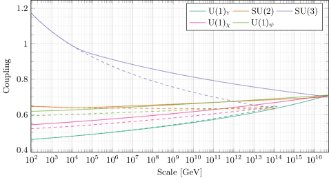
Figure 1: Running of the gauge coupling constants with energy scale calculated at one-loop order. The solid curves show the running when additional scalars charged under $\mathrm{SU}(3)$ are considered as per eq. 6, while the dashed curves consider only the $\mathrm{SU}(3)$ singlets of eq. 5. The additional states used to achieve unification are all introduced at $20\text{\,}\mathrm{TeV}$.

In any gut completion, proton decay would be mediated at least through the $X$ and $Y$ gauge bosons, resulting in a proton lifetime at tree level of

$$\tau_{p}\sim\frac{1}{g^{4}}\frac{m_{X,Y}^{4}}{m_{p}^{5}}.$$ (7)

The $X$ boson mediates the decay $p\to e^{+}\pi^{0}$, while the $Y$ boson can mediate both $p\to e^{+}\pi^{0}$ and $p\to\overline{\nu}K^{+}$. The $X$ and $Y$ bosons gain their masses from the scalar that is responsible for breaking $\mathrm{SU}(5)$ into the sm gauge groups, leading to $m_{X,Y}=gv_{\textsc{gut}}/\sqrt{2}$. Using an estimate from Ref. Langacker (1981) of the proton lifetime that is more accurate than eq. 7, one obtains

$$\tau_{p}\approx\begin{cases}$5.2\text{\times}{10}^{26}\text{\,}\mathrm{yr}$&v_{\textsc{gut}}\sim${10}^{14}\text{\,}\mathrm{GeV}$\\ $3.3\text{\times}{10}^{37}\text{\,}\mathrm{yr}$&v_{\textsc{gut}}\sim${10}^{16}\text{\,}\mathrm{GeV}$\end{cases},$$ (8)

using our value of the gauge coupling constant $g$ at the unification scale. At present, Super-Kamiokande has found that $\tau/\operatorname{Br}(p\to e^{+}\pi^{0})>$8.2\text{\times}{10}^{33}\text{\,}\mathrm{yr}$$ Asakura et al. (2015), and KamLAND has found that $\tau(p\to\overline{\nu}K^{+})>$5.4\text{\times}{10}^{32}\text{\,}\mathrm{yr}$$ Nishino et al. (2009). Thus the scenario of eq. 6 is clearly phenomenologically allowed.

II.2 Decay of Exotic Quarks

The exotic quarks in $\chi_{5,\overline{5}}$ pose a problem in this model as they cannot decay at tree level. In a gut completion of this model, the decay can take place through the coloured components of $H_{5,\overline{5}}$ quintuplets, though the decay width will remain small as the coloured Higgs components are required to be extremely heavy in order to evade constraints from proton decay. Having long-lived coloured exotic particles is problematic as it interferes with nucleosynthesis and as a result, the lifetime of the exotic quarks needs to be less than $0.1\text{\,}\mathrm{s}$ Kawasaki et al. (2005); Reno and Seckel (1988).

At dimension five (d5), the only gauge-invariant term contributing to the decay of the exotic quarks is

$$\mathcal{L}_{\textsc{d5}}\supset\frac{1}{\Lambda}\Phi_{1}^{\dagger}\Phi_{2}^{\dagger}\chi_{5}\psi_{\overline{5}}$$ (9)

which introduces mixing between the sm and exotic down-type quarks. We will be assuming that the mixing is confined within each generation so that it is sufficient to consider the $2\times 2$ mixing:

$$\mathcal{L}_{d-B} =\begin{pmatrix}\overline{d}_{\textsc{l}}&\overline{B}_{\textsc{l}}\end{pmatrix}\begin{pmatrix}m_{d}&0\\ \frac{v_{1}v_{2}}{2\Lambda}&m_{B}\end{pmatrix}\begin{pmatrix}d_{\textsc{r}}\\ B_{\textsc{r}}\end{pmatrix}+\text{h.c.}$$ (10a)

$$=\begin{pmatrix}\overline{d}^{\prime}_{\textsc{l}}&\overline{B}^{\prime}_{\textsc{l}}\end{pmatrix}U_{\textsc{l}}\begin{pmatrix}m_{d}^{\prime}&0\\ 0&m_{B}^{\prime}\end{pmatrix}U_{\textsc{r}}^{\dagger}\begin{pmatrix}d^{\prime}_{\textsc{r}}\\ B^{\prime}_{\textsc{r}}\end{pmatrix}+\text{h.c.},$$ (10b)

where the primed fields denote the mass eigenstates, and $m_{d}$ and $m_{B}$ are the original masses generated from the Yukawa interactions with the Higgs and $\Phi_{1}$ respectively. This mixing introduces a small mass correction to the two original masses:

$$m_{d}^{\prime}-m_{d} =-\frac{1}{2}\left(\frac{v_{1}v_{2}}{2\Lambda}\right)^{2}\frac{m_{d}}{m_{B}^{2}},$$ (11a)

$$m_{B}^{\prime}-m_{B} =\frac{1}{2}\left(\frac{v_{1}v_{2}}{2\Lambda}\right)^{2}\frac{1}{m_{B}}.$$ (11b)

For the parameters investigated, the resulting correction to the down-type sm quarks is about 1 part in ${10}^{10}$ at most. We are taking $\Lambda$ to be the gut scale, ${10}^{16}\text{\,}\mathrm{GeV}$.

The $d$–$B$ quark mixing introduces new terms allowing for the exotic quarks to decay to $Wu$, $Zd$ and $Hd$ and resulting in a decay width

$$\Gamma_{\textsc{d5}}(B)\sim\left(\frac{v_{1}v_{2}}{2\Lambda}\right)^{2}\frac{1}{m_{B}}.$$ (12)

The tree-level partial widths are described in the appendix, along with the relevant couplings to the $W$ and $Z$ gauge bosons, and the Higgs boson. In collider searches, we will be primarily interested in final states involving third-generation sm quarks, in which case the branching fractions as functions of the exotic quark mass are plotted in fig. 2 assuming the benchmark configuration of vevs described in section III.1 ($v_{1}=$23\text{\,}\mathrm{TeV}$$, $v_{2}=$25\text{\,}\mathrm{TeV}$$).

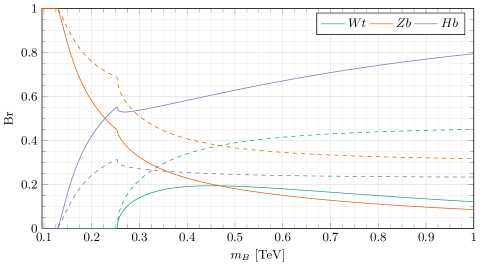
Figure 2: Decay branching ratios of the third generation exotic quark into third generation sm quarks. In the solid lines, the vev of $\Phi_{3}$ is taken to be ${10}^{9}\text{\,}\mathrm{GeV}$ so that the exotic quarks decay promptly. The dashed lines indicate the branching ratios in the absence of $\Phi_{3}$. Decays mediated by virtual particles are not included.

In order to satisfy the Big Bang nucleosynthesis (bbn) constraint, $v_{1,2}$ must be at least in the low $\mathrm{TeV}$ range; however due to the decreased $d$–$B$ mixing with larger mass separation, there is an upper bound on the exotic quark masses for a given $v_{1}$ and $v_{2}$. In particular, the benchmark configuration of vevs requires that $m_{B}<$3\text{\,}\mathrm{TeV}$$ as can be seen in fig. 3. The remaining range of allowed masses results in collider-stable exotic quarks.

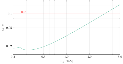
Figure 3: Lifetime of the exotic $B$ quarks for the benchmark vev configuration from section III.1. In red is the upper bound on the lifetime of the exotic quarks due to bbn Kawasaki et al. (2005); Reno and Seckel (1988).

In Ref. Cai et al. (2016), an additional scalar $\Phi_{3}$ was introduced in order to facilitate the decay of the exotic quarks in case the vevs of $\Phi_{1}$ and $\Phi_{2}$ were insufficient to satisfy the bbn constraints. The quantum numbers of $\Phi_{3}$ are shown in table 1(b), and it introduces the following additional d5 terms that facilitate the decay of the exotic quark:

$$\mathcal{L}_{\textsc{d5}}\supset\frac{1}{\Lambda}\left[\Phi_{1}\Phi_{3}^{\dagger}\chi_{5}\psi_{\overline{5}}+\Phi_{3}H_{\overline{5}}\chi_{5}\psi_{10}\right].$$ (13)

The first term introduces another contribution to the off-diagonal entry in the mass matrix in eq. 10a, while the second term introduces direct coupling between the Higgs, bottom quark and exotic quark after $\Phi_{3}$ gains a vev. As this last term is not suppressed by the decreased mixing that accompanies larger $d$–$B$ mass separations, the decay $B\to Hd$ becomes the dominant decay mode for heavy exotic quark masses and scales according to

$$\Gamma_{\textsc{d5}}(B\to Hd)\sim\left(\frac{v_{3}}{\Lambda}\right)^{2}m_{B}.$$ (14)

The branching fraction to $B\to Hd$ reaches $90\text{\,}\mathrm{\char 37\relax}$ at $m_{B}=$1.7\text{\,}\mathrm{TeV}$$ and $95\text{\,}\mathrm{\char 37\relax}$ at $2.6\text{\,}\mathrm{TeV}$ for the benchmark configuration of vevs and $v_{3}=${10}^{9}\text{\,}\mathrm{GeV}$$.

II.3 Neutrino Masses and Mixing

Below the electroweak scale and remaining in the one-generation approximation, there are five neutral fermions which will mix and generate the seesaw mechanism. Their mass matrix in the $(\psi_{\overline{5}},\psi_{1},\chi_{\overline{5}},\chi_{5},\chi_{1})$ basis is

$$\mathrm{M}_{\nu}=\frac{1}{\sqrt{2}}\begin{pmatrix}0&-y_{\nu}v_{u}&0&0&0\\ -y_{\nu}v_{u}&0&0&0&y_{2}v_{2}\\ 0&0&0&y_{1\ell}v_{1}&-y_{xu}v_{u}\\ 0&0&y_{1\ell}v_{1}&0&-y_{xd}v_{d}\\ 0&y_{2}v_{2}&-y_{xu}v_{u}&-y_{xd}v_{d}&0\end{pmatrix}.$$ (15)

The different signs within the mass matrix arise due to the differences in the $\mathrm{SU}(2)$ contractions. For example, the sm neutrino mass term with $\mathrm{SU}(2)$ indices explicitly written is

$$y_{\nu}H_{u}^{\alpha}\overline{L}^{\beta}\psi_{1}\varepsilon_{\alpha\beta}\equiv y_{\nu}\left[H_{u}^{-}\overline{e}_{\textsc{l}}-H_{u}^{0}\overline{\nu}_{\textsc{l}}\right]\psi_{1}.$$ (16)

In the case of the $y_{1\ell}$ and $y_{2}$ Yukawa terms, the sign is positive because all fields are $\mathrm{SU}(2)$ singlets.

With $v_{1}$ and $v_{2}$ both much larger than $v_{u,d}$, one mass eigenstate will be very light, two will be $\sim v_{1}$ and two will be $\sim v_{2}$. The latter two pairs form pseudo-Dirac fermions with small mass splittings. In the scenario where $y_{1\ell}v_{1}$ and $y_{2}v_{2}$ are nondegenerate and both larger than all other terms in the mass matrix (eq. 15), the mass eigenstates of all the neutrinos are well approximated by:

$$m_{\nu} \approx\frac{\sqrt{2}y_{\nu}^{2}y_{xd}y_{xu}}{y_{1\ell}y_{2}^{2}}\frac{v_{d}v_{u}^{3}}{v_{1}v_{2}^{2}},$$ (17a)

$$m_{N_{1}} \approx\frac{y_{1\ell}v_{1}}{\sqrt{2}},$$ (17b)

$$m_{N_{2}} \approx\frac{y_{2}v_{2}}{\sqrt{2}}.$$ (17c)

Alternatively the mass scale of the sm neutrinos can be expressed as

$$m_{\nu}\approx\frac{y_{\nu}^{2}y_{xd}y_{xu}}{2}\frac{v_{\textsc{sm}}^{4}}{m_{N_{1}}m_{N_{2}}^{2}}\cos\beta\sin^{3}\beta,$$ (18)

where $\tan\beta\vcentcolon=v_{u}/v_{d}$ and $m_{N_{1,2}}$ are taken to be exactly as given in eqs. 17b and 17c. It should be re-iterated that, in general, the exact mass eigenstates ought to be calculated from the matrix itself as the above expressions are only true in certain limiting cases. For example, in scenarios where $y_{1\ell}v_{1}\sim v_{2}v_{2}$ the above approximations no longer hold. Additionally, certain small contributions have been omitted in the expressions above as they are generally insignificant. For example, there are higher-order terms in $m_{\nu}$ which are suppressed by larger factors of $v_{1,2}$, and the two pseudo-Dirac masses in $m_{N_{1,2}}$ have small contributions proportional to $v_{u,d}$.

The masses were calculated by setting the Yukawa couplings in eq. 15 at the gut scale and running them down to low scales using one-loop rges. Due to the smallness of sm neutrino masses, corrections occurring at two-loop order have a possibility of introducing sizeable corrections to the light neutrino masses, though in our case no such issues were encountered: the masses of the sm neutrinos received only a minor correction.

Current constraints from Planck place an upper bound of $290\text{\,}\mathrm{meV}$ on the sum of light neutrino masses Planck Collaboration (2016), while current best fits on neutrino observables Capozzi et al. (2017) require that the sum of light neutrino masses be at least $60\text{\,}\mathrm{meV}$ and $100\text{\,}\mathrm{meV}$ for the normal and inverted hierarchies respectively.

This model easily achieves light neutrino masses on the order of $10\text{\,}\mathrm{meV}$ while avoiding having extremely small Yukawa couplings. For example, with $\tan\beta=10$, the values of the product $y_{xu}y_{xd}y_{\nu}^{2}$ which will generate a neutrino mass of $50\text{\,}\mathrm{meV}$ are shown in fig. 4. Even in the case where exotic neutrinos masses are $\sim$100\text{\,}\mathrm{GeV}$$, we can realize the desired lightness of the sm neutrinos provided that $y_{xu}y_{xd}y_{\nu}^{2}\approx(${10}^{-3}$)^{4}$.

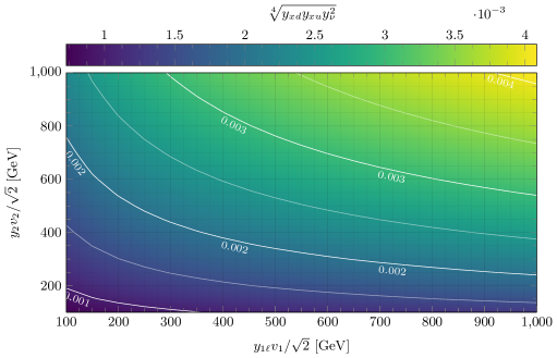
Figure 4: Values of the geometric mean of the four Yukawa couplings which will generate a neutrino mass of $50\text{\,}\mathrm{meV}$ assuming that $\tan\beta=10$, as a function of the two exotic neutrino masses. The seesaw mechanism can easily be achieved with relatively light exotic neutrinos and Yukawa couplings similar to those found in the sm. The white contour lines show specific values of $\sqrt[4]{y_{xd}y_{xu}y_{\nu}^{2}}$.

The sm neutrinos mix primarily with $\psi_{1}$ and $\chi_{1}$, and only negligibly with the neutral components of $\chi_{5,\overline{5}}$ even if these are much lighter than $\psi_{1}$ and $\chi_{1}$ (though still assuming they are significantly heavier than the sm neutrinos) making it sufficient to consider the simplified neutrino mass matrix,

$$\frac{1}{\sqrt{2}}\begin{pmatrix}0&-y_{\nu}v_{u}&0\\ -y_{\nu}v_{u}&0&y_{2}v_{2}\\ 0&y_{2}v_{2}&0\end{pmatrix},$$ (19)

when evaluating the mixing between the sm neutrinos and exotic neutrinos. In particular, the mixing of sm neutrinos with exotic neutrinos is largely independent of $y_{1\ell}v_{1}$ despite the sm neutrino mass being proportional to $1/y_{1\ell}v_{1}$. This results in the neutrino mixing and neutrino masses not being as strongly linked as in the conventional seesaw mechanism, thereby allowing this model to have simultaneously large mixing and quite small mass separations. Another consequence is that the mixing of the sm neutrino need not be primarily with the lightest exotic neutrino.

This mixing with exotic neutrinos causes the Pontecorvo–Maki–Nakagawa–Sakata (pmns) matrix to deviate from unitarity which has repercussions for a number of lepton flavour and electroweak observables. Following the notation of Ref. Fernandez-Martinez et al. (2016), this deviation from unitarity can be encapsulated in $\eta$ defined by:

$$N=(I-\eta)U_{\textsc{pmns}},$$ (20)

where $N$ is the matrix describing the mixing between the light neutrino mass eigenstates and the sm charged leptons via $W$ interactions. In the one-generation approximation, the deviation from unitarity is

$$2\eta_{\alpha\alpha}=\left[1+\left(\frac{y_{2}v_{2}}{y_{\nu}v_{\textsc{sm}}\sin\beta}\right)^{2}\right]^{-1}.$$ (21)

A global fit to lepton flavour and electroweak data places $2\sigma$ upper bounds on $\sqrt{2\eta_{ee}}$, $\sqrt{2\eta_{\mu\mu}}$ and $\sqrt{2\eta_{\tau\tau}}$ of $0.050$, $0.021$ and $0.075$ respectively Fernandez-Martinez et al. (2016). The allowed parameter space in $y_{2}v_{2}$–$y_{\nu}$ is shown in fig. 5 and restricts $y_{\nu}$ to be at most ${10}^{-2}$ if both $\psi_{1}$ and $\chi_{1}$ are around $100\text{\,}\mathrm{GeV}$.

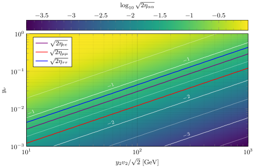
Figure 5: Bound on $y_{\nu}$ and $y_{2}v_{2}$ due to the deviation from unitarity of the pmns matrix based on a global fit to lepton flavour and electroweak data by Fernandez-Martinez et al. (2016). The region of parameter space above the red line is excluded. The bound takes the limit $\tan\beta\to\infty$ and assumes that the neutral components of $\chi_{5,\overline{5}}$ are significantly heavier than the sm neutrinos (though they need not be heavier than $\psi_{1}$ and $\chi_{1}$). The white contour lines show specific values of $\sqrt{2\eta_{\alpha\alpha}}$.

III Constraints

III.1 $Z^{\prime}$ Bosons

In addition to the photon and the sm $Z$ boson, the model features two new massive neutral gauge bosons originating from the exotic $\mathrm{U}(1)$ gauge groups. The most significant contribution to the exotic gauge boson masses originates from the large nonzero vevs of $\Phi_{1,2}$, though as the two Higgs doublets are both charged under these new $\mathrm{U}(1)$ gauge groups, some tree-level mixing between the $Z^{\prime}$ bosons and the sm $Z$ boson is introduced. The matrix of squared masses generated by the symmetry breaking is

$$\mathrm{M}_{Z}=\frac{1}{4}\begin{pmatrix}g_{1}^{2}v_{\textsc{sm}}^{2}&-g_{1}g_{2}v_{\textsc{sm}}^{2}&\frac{g_{1}g_{4}}{\sqrt{5}}v_{\textsc{sm}}^{2}&-\frac{g_{1}g_{5}}{3}v_{\textsc{sm}}^{2}\cos 2\beta\\ -g_{1}g_{2}v_{\textsc{sm}}^{2}&g_{2}v_{\textsc{sm}}^{2}&-\frac{g_{2}g_{4}}{\sqrt{5}}v_{\textsc{sm}}^{2}&\frac{1}{3}g_{2}g_{5}v_{\textsc{sm}}^{2}\cos 2\beta\\ \frac{g_{1}g_{4}}{\sqrt{5}}v_{\textsc{sm}}^{2}&-\frac{g_{2}g_{4}}{\sqrt{5}}v_{\textsc{sm}}^{2}&\frac{g_{4}^{2}}{20}(25v_{2}^{2}+4v_{\textsc{sm}}^{2})&\frac{g_{4}g_{5}}{12\sqrt{5}}(25v_{2}^{2}-4v_{\textsc{sm}}^{2}\cos 2\beta)\\ -\frac{g_{1}g_{5}}{3}v_{\textsc{sm}}^{2}\cos 2\beta&\frac{1}{3}g_{2}g_{5}v_{\textsc{sm}}^{2}\cos 2\beta&\frac{g_{4}g_{5}}{12\sqrt{5}}(25v_{2}^{2}-4v_{\textsc{sm}}^{2}\cos 2\beta)&\frac{g_{5}^{2}}{36}(16v_{1}^{2}+25v_{2}^{2}+4v_{\textsc{sm}}^{2})\end{pmatrix}$$ (22)

The mixing between the sm and exotic bosons introduces a modification to the $Z$ pole mass and couplings to fermions which have both been measured very precisely, with the $Z$ pole mass measurements significantly constraining the $Z$–$Z^{\prime}$ mixing Langacker (2009). At tree level, the correction to the $Z$ pole mass in this model is

$$\frac{m_{Z,\textsc{sm}}^{2}-m_{Z}^{2}}{m_{Z,\textsc{sm}}^{2}}\approx\frac{4v_{\textsc{sm}}^{2}}{25v_{2}^{2}}+\frac{v_{\textsc{sm}}^{2}}{v_{1}^{2}}\frac{1}{(1+\tan^{2}\beta)^{2}},$$ (23)

where $m_{Z,\textsc{sm}}^{2}$ is the sm tree-level $Z$ boson mass, $m_{Z}^{2}$ is the tree-level mass in this model, and we are assuming $v_{\textsc{sm}}\ll v_{1,2}$. The $Z$ boson pole mass has been measured accurately at lep with the best fit being $91.1875(21)\text{\,}\mathrm{GeV}$ The Aleph Collaboration et al. (2006). In order that the shift to the $Z$ pole be such that the $Z$ pole remain within $1\sigma$ of the experimental value, we require that $v_{2}$ be larger than $14.5\text{\,}\mathrm{TeV}$ (taking $\tan\beta\to\infty$).

The shift in the $Z$ pole mass also introduces a shift in the electroweak $\rho$ parameter,

$$\rho\vcentcolon=\frac{m_{W}^{2}}{m_{Z}^{2}\cos^{2}\theta_{\textsc{W}}},$$ (24)

where $\theta_{\textsc{W}}\vcentcolon=\arctan(g_{2}/g_{1})$. The best fit for this parameter was determined by lep to be $1.0050(10)$ The Aleph Collaboration et al. (2006), and just as with the pole mass, requiring that the shift in $\rho$ not exceed the standard deviation of the measured value results in a lower bound on $v_{2}$ of $3.1\text{\,}\mathrm{TeV}$.

If we demand that the gauge couplings unify at the gut scale, this fixes the interaction of the $Z^{\prime}$ bosons with $\Phi_{1,2}$ and the other fermions and consequently the masses of both $Z^{\prime}$ bosons are only determined by the vevs of $\Phi_{1,2}$. Additionally, the decays of the $Z^{\prime}$ bosons are similarly fixed and depend only on the kinematics of the decays (and consequently the exotic Yukawa couplings).

Depending on the exact masses of the exotic fermions, the lighter $Z^{\prime}$ boson mass is restricted to be above $2.8\text{\,}\mathrm{TeV}3.4\text{\,}\mathrm{TeV}$ as shown in fig. 6. This limit on the vev configurations also implies that the heavier $Z^{\prime}$ boson mass be at least $7.7\text{\,}\mathrm{TeV}$. For the remainder of this paper, we will consider the benchmark point $v_{1}=$23\text{\,}\mathrm{TeV}$$ and $v_{2}=$25\text{\,}\mathrm{TeV}$$ for definiteness. For this configuration, the masses of the two $Z^{\prime}$ bosons are $3.4\text{\,}\mathrm{TeV}10.3\text{\,}\mathrm{TeV}$. In the future, the completion of lhc $14\text{\,}\mathrm{TeV}$ runs could provide enough data to exclude the $Z^{\prime}$ boson mass up to $6\text{\,}\mathrm{TeV}$, and prospects at a $100\text{\,}\mathrm{TeV}$ collider could place bounds as high as $30\text{\,}\mathrm{TeV}$ on the $Z^{\prime}$ masses Arcadi et al. (2017).

As the vevs are actually quite large, this will generally result in large masses for $\Phi_{1}$ and $\Phi_{2}$ unless the quartic coupling constants in the scalar potential are tuned to achieve light masses. Additionally, neither scalar can be easily produced at the lhc as they couple to neither gluons nor the sm quarks at tree level. In the case of $\Phi_{1}$, it can couple to gluons through a loop of exotic quarks; however, the effective $\Phi_{1}gg$ coupling is generally insignificant as either the exotic masses are too heavy and suppress the loop factor, or the Yukawa coupling is too small.

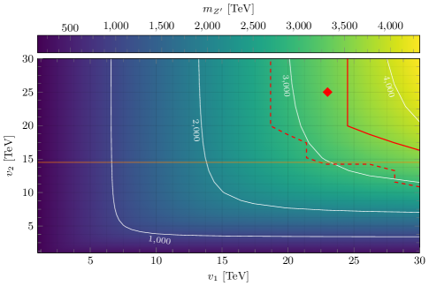
Figure 6: Lower bounds on the vevs of $\Phi_{1}$ and $\Phi_{2}$. The orange line indicates the lower bound on $v_{2}$ due to modification to the $Z$ pole mass (taking $\tan\beta\to\infty$) and the red lines show the bounds from the $pp\to Z^{\prime}\to\ell\ell$ channel ($\ell=e,\leavevmode\nobreak\ \mu$) based on the analysis in Ref. Atlas collaboration (2017)—lighter $Z^{\prime}$ masses being excluded. The red solid and dashed lines show the exclusion with $y_{1d}=y_{1\ell}=y_{2}=0.5$ and $y_{1d}=y_{1\ell}=y_{2}=$5\text{\times}{10}^{-3}$$ at the gut scale making the exotic fermions heavy and light, respectively. The white contours indicate specific values of $m_{Z^{\prime}}$. The point marked by the diamond indicates the benchmark configuration of vevs investigated in this model.

III.2 Exotic Down Quarks

The exotic quarks introduced in this model can be abundantly produced at the lhc thanks to their couplings to gluons and provide one of the main phenomenological windows into this model. Their detection however depends primarily on their decay mode which, as discussed in section II.2, will be collider-stable in the absence of $\Phi_{3}$.

Specifically, with the benchmark vev configuration, the lifetime of the exotic quarks is $\sim$ $20\text{\,}\mathrm{ms}$ for $m_{B}\sim$ $500\text{\,}\mathrm{GeV}$. With the introduction of $\Phi_{3}$, the exotic quarks can decay promptly provided $v_{3}\gtrsim${10}^{9}\text{\,}\mathrm{GeV}$$.

In the scenario where $\Phi_{3}$ is absent, the exotic quarks hadronize and form colorless hadrons analogous to $R$-hadrons after being created. As the hadrons traverse the detector, they leave tracks with large energy losses due to ionization which have been searched for by both Atlas Atlas Collaboration (2016a, b) and Cms Cms Collaboration (2016a). As we are assuming for simplicity that all the exotic quarks have the same mass, the cross section is enhanced by a factor of 3 leading to slightly more stringent bounds on the quark mass as shown in fig. 7.

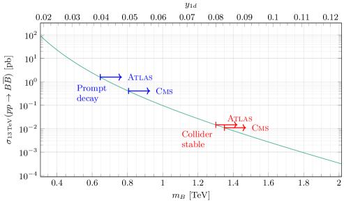
Figure 7: Lower bounds on exotic quark masses. The Yukawa coupling on the top axis assumes $v_{1}=$23\text{\,}\mathrm{TeV}$$. In red are the bounds on collider-stable exotic quarks from Atlas Atlas Collaboration (2016b) and Cms Cms Collaboration (2016a), and in blue are the bounds on promptly decaying exotic quarks from Atlas Atlas Collaboration (2017) and Cms Cms Collaboration (2016b). The green line shows the predicted production cross section of the exotic quarks at the lhc at a centre-of-mass energy of $13\text{\,}\mathrm{TeV}$, with the multiplicity from the three generations taken into account.

If the scalar $\Phi_{3}$ is introduced (despite not being explicitly needed to satisfy the nucleosynthesis constraint), the exotic quarks will decay promptly provided $v_{3}\gtrsim${10}^{9}\text{\,}\mathrm{GeV}$$. In this case, searches by Atlas and Cms have nearly exclusively searched for decays into third-generation sm quarks as the heavy sm quarks provide a way to distinguish the exotic quark decays from other background events. The resulting limits on exotic quarks depend primarily on the three decay modes:

$$B\to Wt, B\to Zb, B\to Hb.$$

Although the d5 terms allowing for the exotic quarks to decay could have complex flavour couplings, we will assume that the three generations of exotic quarks decay into sm fermions of their corresponding generations. The branching ratios to the three final states above are shown shown in fig. 2 where the enhancement of $\operatorname{Br}(B\to Hb)$ due to the second term in eq. 13 is evident. The explicit partial widths are listed in the appendix.

The most stringent constraints come from a search by Cms in Ref. Cms Collaboration (2016b) which has been particularly sensitive to decays involving a Higgs, ultimately excluding masses of the third generation below $810\text{\,}\mathrm{GeV}$. A more recent analysis by Cms with data collected at $\sqrt{s}=$13\text{\,}\mathrm{TeV}$$ has failed to improve the bounds on the exotic down-type quarks Cms Collaboration (2017a).

Searches by Atlas have generally been focusing on final states involving a boosted $W$ boson resulting in weaker constraints on the exotic quarks presented in this model. Their most recent analysis in Ref. Atlas Collaboration (2017) restricted the limits of the third generation of exotic quarks to $650\text{\,}\mathrm{GeV}$. Atlas has also conducted a search with light sm quarks in the final states Atlas Collaboration (2015a), but this failed to place any constraints on the exotic quarks in this model as the search was insensitive to $B\to Hq$.

III.3 Exotic Leptons & Neutrinos

In the conventional seesaw mechanisms, the new leptons and neutrinos are typically well out of the reach of present-day experiments. In some circumstances, this can be alleviated by modifying the textures of the Dirac (and Majorana) mass matrices allowing these models to be experimentally probed more easily Deppisch et al. (2015). In this $\mathrm{E}_{6}$-inspired model, the exotic leptons can have electroweak-scale masses while still achieving the desired suppression of the light neutrino masses. This makes it in principle possible to produce them at the lhc, though in most cases the production cross section is too small for these states to be observed over the backgrounds.

Searches at lep have limited the masses of the exotic charged leptons to be above $102\text{\,}\mathrm{GeV}$ L3 Collaboration (2001). The same analysis also restricted the masses of exotic neutrinos that decay into a $W$ to also be above $102\text{\,}\mathrm{GeV}$. Of the four exotic neutrinos per generation, only one pair of gauge eigenstates are charged under $\mathrm{SU}(2)$, but through mixing, all mass eigenstates ultimately decay into a $W$ boson (provided it is kinematically allowed) and a charged lepton.

Searches for heavy neutrinos have been conducted by both Atlas Atlas Collaboration (2015b) and Cms Cms Collaboeration (2017); Cms Collaboration (2017b, 2016c, 2015). These were performed in the context of other seesaw models, though in all cases, they selected for events with the topology shown in fig. 8(a). Often, searches look for same-sign leptons and also different-flavour lepton as the sm backgrounds are low in both cases. Unfortunately, the cross section $\sigma(pp\to\ell N)$ is generally too small as it is suppressed by the neutrino mixing. As discussed in section II.3, it is possible to have quite a considerable mixing though this is bounded by precision lepton flavour and electroweak observables. For regions which are not already excluded by lep and the precision observables, the production cross section at $13\text{\,}\mathrm{TeV}$ reaches at most ${10}^{-3}\text{\,}\mathrm{pb}$ which is too small to be observed at the lhc over the sm backgrounds.

[small, horizontal=w1 to w2, layered layout] q1 [particle=$q$] – [fermion] w1, q2 [particle=$\overline{q}$] – [anti fermion] w1, w1 – [boson, edge label=$W$] w2, w2 – [fermion] l1 [particle=$\ell^{\pm}$], w2 – [fermion, edge label’=$N$] n, n – [boson, edge label’=$W$] wn, wn – [fermion] qf1 [particle=$q$] , wn – [anti fermion] qf2 [particle=$\overline{q}$], n – [fermion] l2 [particle=$\ell^{\pm}$], ;

(a) Topology used in searches for heavy neutrinos. This can result in same-sign dilepton of different flavours making it more easily identifiable.

[small, horizontal=w1 to w2, layered layout] q1 [particle=$q$] – [fermion] w1, q2 [particle=$\overline{q}$] – [anti fermion] w1, w1 – [boson, edge label=$W$] w2, w2 – [fermion, edge label=$r^{\pm}$] l1, l1 – [boson, edge label’=$W$] wl, l1 – [fermion] nu [particle=$\nu_{\textsc{sm}}$], wl – [anti fermion] ql2 [particle=$\overline{q},\ell^{\pm}$], wl – [fermion] ql1 [particle=$q,\nu$], w2 – [fermion, edge label’=$N$] n, n – [boson, edge label=$W$] wn, wn – [fermion] qn1 [particle=$q,\nu$] , wn – [anti fermion] qn2 [particle=$\overline{q},\ell^{\mp}$], n – [fermion] l2 [particle=$\ell^{\pm}$], ;

(b) Most likely topology to use in searches for the exotic lepton doublet.

Figure 8: Topologies involved in searches for the exotic leptons.

On the other hand, the production of the exotic lepton doublet can be much larger as it is generally not suppressed by the neutrino mixing. The topology of the event in this case is more complex, which would consist of two $W$ bosons, one lepton, and missing $E_{T}$ as shown in fig. 8(b). The $W$ bosons could either decay hadronically which would facilitate the event reconstruction, or they could decay to different-flavour leptons in order to avoid sm background though at the cost of having several neutrinos in the final state. Nevertheless, the production cross section for this topology is of order $0.1\text{\,}\mathrm{pb}$ at best in regions which are not excluded by lep, and falls off very rapidly as the masses of the leptons are increased.

Although this model does not present a clear way to detect the heavy neutrinos directly, the phenomenology presented by the remaining exotic particle content can provide indirect bounds on the heavy neutrino masses. In particular, we have not been imposing that the Yukawa couplings unify at the gut scale, though a complete model must evidently do so. If we require that $y_{1d}=y_{1\ell}$ at the gut scale, the bounds on the exotic quarks discussed in section III.2 translate to a bound of $y_{1\ell}>$0.040$$ ($m_{r},m_{N_{1}}>$650\text{\,}\mathrm{GeV}$$) in the collider-stable case, and $y_{1\ell}>$0.024$$ ($m_{r},m_{N_{1}}>$390\text{\,}\mathrm{GeV}$$) in the prompt-decay case.

III.4 Higgs Sector

The two Higgs doublets contained within the scalar sector correspond to the well-studied type-ii 2hdm (see Refs. Bhattacharyya and Das (2016); Branco et al. (2012) for recent reviews) in which one gauge eigenstate couples to up-type quarks (and neutrinos), and the other couples to down-type quarks and electrons. The terms of the scalar potential concerning the Higgs doublets are

$$\begin{split}&\mathcal{V}=-\mu_{u}^{2}H_{u}^{\dagger}H_{u}-\mu_{d}^{2}H_{d}^{\dagger}H_{d}+\lambda_{u}(H_{u}^{\dagger}H_{u})^{2}+\lambda_{d}(H_{d}^{\dagger}H_{d})^{2}\\ &+\lambda_{ud}(H_{u}^{\dagger}H_{u})(H_{d}^{\dagger}H_{d})+\lambda_{ud}^{\prime}(H_{d}^{\dagger}H_{u})(H_{u}^{\dagger}H_{d})-\left[\kappa\Phi_{1}H_{u}H_{d}+\text{h.c.}\right]\end{split}$$ (25)

After $\Phi_{1}$ gains a vev, the last term generates the term $\mu_{ud}^{2}\vcentcolon=\kappa v_{1}/\sqrt{2}$ (also referred to as $m_{12}$ in the literature). As discussed in section III.1, there already exists a lower limit on $v_{1}$ of $\sim$23\text{\,}\mathrm{TeV}$$, thus $\mu_{ud}$ can easily be large. Having said this, the limit $\kappa\to 0$ is technically natural as it breaks an accidental global $\mathrm{U}(1)$ symmetry, and thus it is not regenerated through radiative corrections and can be small. The $(H_{u}^{\dagger}H_{d})^{2}$ term present in conventional 2hdm models is forbidden here as it is not gauge invariant under the additional $\mathrm{U}(1)$ gauge groups. As a result, the only term which is capable of introducing $CP$ violation is $\kappa$, though we will be taking this to be real.

The pseudoscalar and charged scalar squared masses are

$$m_{A}^{2} =\frac{\kappa v_{\textsc{sm}}^{2}\sin 2\beta}{2\sqrt{2}v_{1}}+\frac{\sqrt{2}\kappa v_{1}}{\sin 2\beta},$$ (26a)

$$m_{H^{+}}^{2} =\frac{\lambda_{ud}^{\prime}}{2}v_{\textsc{sm}}^{2}+\frac{\sqrt{2}\kappa v_{1}}{\sin 2\beta}.$$ (26b)

Additionally, there are two neutral scalars that arise from 2hdm: $h$ and $H$. One of them is the sm-like Higgs with $m_{h}=$125\text{\,}\mathrm{GeV}$$ and the second scalar will in general be heavier. Their squared masses are

$$m_{h}^{2} \approx\frac{v_{\textsc{sm}}^{2}}{2}\Big{[}\lambda_{d}\cos^{4}\beta+\lambda_{u}\sin^{4}\beta+\lambda_{ud}\sin^{2}2\beta\Big{]},$$ (27a)

$$\begin{split}m_{H}^{2}&\approx\frac{\sqrt{2}\kappa v_{1}}{\sin 2\beta}+\frac{v_{\textsc{sm}}^{2}}{8}\Big{[}\lambda_{d}\sin^{4}2\beta+\lambda_{u}\sin^{4}2\beta-4\lambda_{ud}\sin^{2}2\beta\Big{]},\end{split}$$ (27b)

assuming that the mixing with the $CP$-even components of $\Phi_{1,2}$ can be neglected. With the exception of very small values for $\kappa v_{1}$ and $\tan\beta$, it will in general be the case that $m_{H}\approx m_{H^{+}}\approx m_{A}$.

The rotation of the Higgs doublets from the gauge basis to the mass basis is described by the angle $\alpha$, while the rotation from the gauge basis to the Higgs basis is described by $\beta$ (which has been defined earlier). The Higgs basis is defined such that only one (the sm Higgs) contains the vev. The scenario in which the mass eigenstates line up with the Higgs basis is called the alignment limit and corresponds to $\cos(\alpha-\beta)\to 0$ and deviations from this limit are strongly disfavoured. In this model, the large vev of $\Phi_{1}$ helps to ensure the alignment limit, with

$$\cos(\alpha-\beta)\approx\frac{v_{\textsc{sm}}^{2}}{\sqrt{2}\kappa v_{1}}\frac{\lambda_{u}-2\lambda_{ud}}{\tan^{2}\beta}.$$ (28)

The constraints on 2hdm models were most recently collated in Ref. Arbey et al. (2017). One of the more stringent constraints relevant to type-ii models arises from $b\to s$ transitions which are facilitated by the charged Higgs. Specifically, the latest constraints require that $m_{H^{+}}>$600\text{\,}\mathrm{GeV}$$ for $\tan\beta>1$, and only increase with $\tan\beta<1$.

In the context of collider searches, the pseudoscalar’s coupling to the bottom quarks and $\tau$ leptons is enhanced by larger values of $\tan\beta$. This allows for the pseudoscalar to be produced through a loop of $b$ quarks and subsequently decay to a pair of $\tau$ leptons providing constraints up to $1\text{\,}\mathrm{TeV}$ in the large-$\tan\beta$ regime. The most restrictive constraints from Ref. Arbey et al. (2017) have been recast on the $\tan\beta$–$\kappa v_{1}$ parameter space and are shown in fig. 9, assuming the benchmark configuration of vevs. Values of $\kappa v_{1}$ smaller than $60\text{\times}{10}^{3}\text{\,}\mathrm{G}\mathrm{eV}^{2}$ are generally excluded and larger values of $\tan\beta$ are favoured.

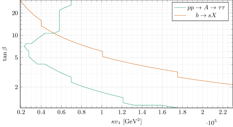
Figure 9: Bounds on the 2hdm sector of the model, presented on the parameters $\tan\beta$ and $\kappa v_{1}$. The lower left area of the plot is excluded. The bounds were recast from Ref. Arbey et al. (2017).

IV Conclusion

In this paper, we have explored the phenomenology of the model presented in Ref. Cai et al. (2016). The primary motivation for this model—the realization of a seesaw mechanism at mass scales testable at the lhc—was achieved without recourse to exceptionally small Yukawa couplings. The additional neutral fermions required to generate the seesaw mechanism are motivated by unification into $\mathrm{E}_{6}$ which, in order to complete the $\bm{27}$ irrep, requires the existence of additional charged leptons and isosinglet quarks as well as two $Z^{\prime}$ bosons. The masses of the exotic fermions are generated by the vevs $v_{1,2}$ of two scalar singlets $\Phi_{1,2}$, and the model also presents a type-ii two-Higgs-doublet model.

A significant constraint on this model arises from searches for $Z^{\prime}$ bosons which restrict the lightest $Z^{\prime}$ mass to be above $2.8\text{\,}\mathrm{TeV}$. As the $Z^{\prime}$ mass is generated by $v_{1,2}$ and the gauge couplings are fixed by requiring that they unify at the gut scale, the $Z^{\prime}$ bound imposes that $v_{1}$ and $v_{2}$ be larger than $18\text{\,}\mathrm{TeV}$ and $15\text{\,}\mathrm{TeV}$ respectively. This will, in general, lead to large masses for the scalar singlets present in this model.

A small amount of mixing between the sm and exotic down-type quarks is generated through a dimension-five term which allows the exotic quarks to decay before bbn, but results in collider-stable quarks. As the mixing is reduced with larger mass separations, bbn imposes an upper bound on the exotic quark masses of $3\text{\,}\mathrm{TeV}$ for the benchmark configuration of vevs investigated in this model, and collider searches for long-lived particles restrict the masses to be above $1.3\text{\,}\mathrm{TeV}$. In order to facilitate the decay of exotic quarks, the authors of Ref. Cai et al. (2016) introduced another scalar which gains a vev. This can allow the exotic quarks to decay promptly if produced at the lhc in which case searches place a lower bound on their masses of $810\text{\,}\mathrm{GeV}$.

Searches for the exotic leptons at the lhc are unfortunately not feasible as the production cross section is generally far too small. In particular, if a prompt sm lepton is required, the process is greatly suppressed by the neutrino mixing. Even the direct production of the exotic charged leptons is generally too small to be seen over the background. As a result, the bound on the leptons remains at $102\text{\,}\mathrm{GeV}$ from searches at lep.

Finally, the model also contains a type-ii 2hdm with the addition of a $\kappa\Phi_{1}H_{u}H_{d}$ interaction in the potential. The large vev of $\Phi_{1}$ helps enforce the alignment limit in the model thereby avoiding most constraints that arise from the 2hdm. Values of $\kappa v_{1}$ below $60\text{\times}{10}^{3}\text{\,}\mathrm{G}\mathrm{eV}^{2}$ are excluded, and larger values of $\tan\beta$ are favoured.

Appendix A $B$ Partial Widths

The mass matrix of the $b$–$B$ quark is shown in eq. 10a, and can be diagonalized using the two unitary matrices $U_{\textsc{l}}$ and $U_{\textsc{r}}$ as shown in eq. 10b where the (un)primed fields denote (gauge) mass eigenstates. We are assuming no mixing between generations so that it is sufficient to deal with a $2\times 2$ mass matrix. When $\Phi_{3}$ is present, the off-diagonal term in eq. 10a becomes $(v_{1}v_{2}+v_{1}v_{3})/2\Lambda$ and for simplicity, we will define $f\vcentcolon=(v_{1}v_{2}+v_{1}v_{3})/2\Lambda$. By taking $v_{3}\to 0$, we recover the scenario where $\Phi_{3}$ is absent.

To leading order in $f$ and $m_{b}/m_{B}$, the two matrices rotating the gauge eigenstates to the mass basis as defined in eq. 10b are

$$U_{\textsc{l}} =\begin{pmatrix}1&f\frac{m_{b}}{m_{B}^{2}}\\ -f\frac{m_{b}}{m_{B}^{2}}&1\end{pmatrix}, U_{\textsc{r}} =\begin{pmatrix}1&f\frac{1}{m_{B}}\\ -f\frac{1}{m_{B}}&1\end{pmatrix}.$$ (29a)

In the gauge basis, the sm and exotic bottom quark couplings to the $W$, $Z$ gauge bosons and the Higgs are,

$$\mathcal{L}_{Z} =\begin{pmatrix}\overline{b}_{\textsc{l}}&\overline{B}_{\textsc{l}}\end{pmatrix}\not{Z}\begin{pmatrix}g^{Z}_{\textsc{l},b}&0\\ 0&g^{Z}_{B}\end{pmatrix}\begin{pmatrix}b_{\textsc{l}}\\ B_{\textsc{l}}\end{pmatrix}+\begin{pmatrix}\overline{b}_{\textsc{r}}&\overline{B}_{\textsc{r}}\end{pmatrix}\not{Z}\begin{pmatrix}g^{Z}_{\textsc{r},b}&0\\ 0&g^{Z}_{B}\end{pmatrix}\begin{pmatrix}b_{\textsc{r}}\\ B_{\textsc{r}}\end{pmatrix},$$ (30a)

$$\mathcal{L}_{W} =\frac{g_{2}}{\sqrt{2}}\begin{pmatrix}\overline{b}_{\textsc{l}}&\overline{B}_{\textsc{l}}\end{pmatrix}\not{W}\begin{pmatrix}1&0\\ 0&0\end{pmatrix}\begin{pmatrix}b_{\textsc{l}}\\ B_{\textsc{l}}\end{pmatrix},$$ (30b)

$$\mathcal{L}_{h} =\frac{h}{\sqrt{2}}\begin{pmatrix}\overline{b}_{\textsc{l}}&\overline{B}_{\textsc{l}}\end{pmatrix}\begin{pmatrix}y_{b}&\frac{v_{3}}{\sqrt{2}\Lambda}\\ 0&0\end{pmatrix}\begin{pmatrix}b_{\textsc{r}}\\ B_{\textsc{r}}\end{pmatrix},$$ (30c)

where the couplings to the $Z$ boson are

$$g^{Z}_{\textsc{l},b} =\frac{1}{60}\mathcal{Z}_{i,2}\begin{pmatrix}-10g_{1}\\ 30g_{2}\\ 3\sqrt{5}g_{4}\\ 5g_{5}\end{pmatrix}_{i}, g^{Z}_{\textsc{r},b} =\frac{1}{60}\mathcal{Z}_{i,2}\begin{pmatrix}20g_{1}\\ 0\\ 9\sqrt{5}g_{4}\\ -5g_{5}\end{pmatrix}_{i}, g^{Z}_{B} =\frac{1}{30}\mathcal{Z}_{i,2}\begin{pmatrix}10g_{1}\\ 0\\ -3\sqrt{5}g_{4}\\ -5g_{5}\end{pmatrix}_{i}.$$ (31a)

in which $\mathcal{Z}$ is the matrix that rotates the neutral gauge bosons into their mass eigenstates [see eq. 22 for the mass matrix] defined such that

$$\begin{pmatrix}\gamma\\ Z\\ Z^{\prime}\\ Z^{\prime\prime}\end{pmatrix}=\mathcal{Z}\begin{pmatrix}A_{\textsc{y}}\\ B_{\mathrm{SU}(2)}\\ A_{\chi}\\ A_{\psi},\end{pmatrix}$$ (32)

$g_{i}$ are the gauge couplings, and $y_{b}$ is the bottom-quark Yukawa. The interactions in the mass basis are then obtained by appropriately rotating the left and right components with $U_{\textsc{l},\textsc{r}}$, after which the resulting partial widths of the exotic quarks are

$$\Gamma(B^{\prime}\to Wt) =\frac{\lambda^{\frac{1}{2}}(m_{B}^{2},m_{W}^{2},m_{t}^{2})}{16\pi}\frac{m_{B}}{m_{W}^{2}}\left\lvert\hat{g}^{W}\right\rvert^{2}\Bigl{[}1+r_{W}^{2}-2r_{t}^{2}-2r_{W}^{4}+r_{t}^{4}+r_{W}^{2}r_{t}^{2}\Bigr{]}$$ (33a)

$$\begin{split}\Gamma(B^{\prime}\to Zb^{\prime})&=\frac{\lambda^{\frac{1}{2}}(m_{B}^{2},m_{Z}^{2},m_{b}^{2})}{16\pi}\frac{m_{B}}{m_{Z}^{2}}\Bigl{[}\\ &\qquad\left(\left\lvert\hat{g}^{Z}_{\textsc{l}}\right\rvert^{2}+\left\lvert\hat{g}^{Z}_{\textsc{r}}\right\rvert^{2}\right)\left(1+r_{Z}^{2}-2r_{b}^{2}-2r_{Z}^{4}+r_{b}^{4}+r_{Z}^{2}r_{b}^{2}\right)\\ &\qquad-12\operatorname{\mathfrak{Re}}[\hat{g}^{Z}_{\textsc{l}}\hat{g}^{Z}_{\textsc{r}}]r_{b}r_{Z}^{2}\Bigr{]}\end{split}$$ (33b)

$$\begin{split}\Gamma(B^{\prime}\to hb^{\prime})&=\frac{\lambda^{\frac{1}{2}}(m_{B}^{2},m_{h}^{2},{m_{b}^{\prime}}^{2})}{16\pi}\frac{1}{m_{B}}\Bigl{[}\left(\left\lvert\hat{y}_{1}\right\rvert^{2}+\left\lvert\hat{y}_{2}\right\rvert^{2}\right)\left(1-r_{h}^{2}+r_{b}^{2}\right)+4\operatorname{\mathfrak{Re}}[\hat{y}_{1}\hat{y}_{2}]r_{b}\Bigr{]}\end{split}$$ (33c)

where $\lambda(x,y,z)$ is the Källén function

$$\lambda(x,y,z)\vcentcolon=x^{2}+y^{2}+z^{2}-2xy-2xz-2yz,$$

$r_{i}\vcentcolon=m_{i}/m_{B}$, and the couplings with circumflexes take into account the rotation to the mass basis. Note that as the corrections to the masses are extremely small [see eq. 11], the distinction between $m_{b,B}$ and $m_{b,B}^{\prime}$ is omitted in the above partial widths. Explicitly, the couplings appearing in eqs. 33a, 33b and 33c are

$$\hat{g}^{W} =f\frac{m_{b}}{m_{B}^{2}}\frac{g_{2}}{\sqrt{2}},$$ (34a)

$$\hat{g}^{Z}_{\textsc{l}} =2f\frac{m_{b}}{m_{B}^{2}}\left(g^{Z}_{B}-g^{Z}_{\textsc{l},b}\right), \hat{g}^{Z}_{\textsc{r}} =2f\frac{1}{m_{B}}\left(g^{Z}_{\textsc{r},b}-g^{Z}_{B}\right),$$ (34b)

$$\hat{y}_{1} =-f\frac{1}{m_{B}}\frac{y_{b}}{\sqrt{2}}-f^{2}\frac{1}{m_{B}}\frac{m_{b}}{m_{B}^{2}}\frac{v_{3}}{2\Lambda}, \hat{y}_{2} =-f\frac{m_{b}}{m_{B}^{2}}\frac{y_{b}}{\sqrt{2}}+\frac{v_{3}}{2\Lambda}.$$ (34c)

References

- Minkowski (1977) P. Minkowski, Phys. Lett. B 67, 421 (1977).
- Yanagida (1979) T. Yanagida, in Proceedings: Workshop on the Unified Theories and the Baryon Number in the Universe: Tsukuba, Japan, February 13-14, 1979, Vol. C7902131 (1979) pp. 95–99.
- Gell-Mann et al. (1979) M. Gell-Mann, P. Ramond, and R. Slansky, in Supergravity Workshop Stony Brook, New York, September 27-28, 1979, Vol. C790927 (1979) pp. 315–321, arXiv:1306.4669 [hep-th] .
- Mohapatra and Senjanović (1980) R. N. Mohapatra and G. Senjanović, Phys. Rev. Lett. 44, 912 (1980).
- Foot et al. (1989) R. Foot, H. Lew, X. G. He, and G. C. Joshi, Z. Phys. C44, 441 (1989).
- Magg and Wetterich (1980) M. Magg and C. Wetterich, Phys. Lett. 94B, 61 (1980).
- Schechter and Valle (1980) J. Schechter and J. W. F. Valle, Phys. Rev. D22, 2227 (1980).
- Cheng and Li (1980) T. P. Cheng and L.-F. Li, Phys. Rev. D22, 2860 (1980).
- Lazarides et al. (1981) G. Lazarides, Q. Shafi, and C. Wetterich, Nucl. Phys. B181, 287 (1981).
- Wetterich (1981) C. Wetterich, Nucl. Phys. B187, 343 (1981).
- Mohapatra and Senjanovic (1981) R. N. Mohapatra and G. Senjanovic, Phys. Rev. D23, 165 (1981).
- Cai et al. (2016) Y. Cai, J. D. Clarke, R. R. Volkas, and T. T. Yanagida, Phys. Rev. D 94, 033003 (2016).
- Gürsey et al. (1976) F. Gürsey, P. Ramond, and P. Sikivie, Phys. Lett. B 60, 177 (1976).
- Achiman and Stech (1978) Y. Achiman and B. Stech, Phys. Lett. 77B, 389 (1978).
- Shafi (1978) Q. Shafi, Phys. Lett. 79B, 301 (1978).
- Barbieri et al. (1981) R. Barbieri, D. V. Nanopoulos, and A. Masiero, Phys. Lett. 104B, 194 (1981).
- Bajc and Susič (2014) B. Bajc and V. Susič, J. High Energy Phys. 2014, 58 (2014).
- Babu et al. (2015) K. S. Babu, B. Bajc, and V. Susič, J. High Energy Phys. 2015, 108 (2015).
- Staub (2014) F. Staub, Comput. Phys. Commun. 185, 1773 (2014).
- Porod and Staub (2012) W. Porod and F. Staub, Comput. Phys. Commun. 183, 2458 (2012).
- Athron et al. (2015) P. Athron, J.-H. Park, D. Stöckinger, and A. Voigt, Comput. Phys. Commun. 190, 139 (2015).
- Langacker (1981) P. Langacker, Phys. Rep. 72, 185 (1981).
- Asakura et al. (2015) K. Asakura et al., Phys. Rev. D 92, 052006 (2015).
- Nishino et al. (2009) H. Nishino et al., Phys. Rev. Lett. 102, 141801 (2009).
- Kawasaki et al. (2005) M. Kawasaki, K. Kohri, and T. Moroi, Phys. Rev. D 71, 083502 (2005).
- Reno and Seckel (1988) M. H. Reno and D. Seckel, Phys. Rev. D 37, 3441 (1988).
- Mohapatra and Valle (1986) R. N. Mohapatra and J. W. F. Valle, Proceedings, 23RD International Conference on High Energy Physics, JULY 16-23, 1986, Berkeley, CA, Phys. Rev. D34, 1642 (1986).
- Gonzalez-Garcia and Valle (1989) M. C. Gonzalez-Garcia and J. W. F. Valle, Phys. Lett. B216, 360 (1989).
- Planck Collaboration (2016) Planck Collaboration, Astron. Astrophys. 594, A13 (2016).
- Capozzi et al. (2017) F. Capozzi, E. Di Valentino, E. Lisi, A. Marrone, A. Melchiorri, and A. Palazzo, Phys. Rev. D 95, 096014 (2017).
- Fernandez-Martinez et al. (2016) E. Fernandez-Martinez, J. Hernandez-Garcia, and J. Lopez-Pavon, J. High Energy Phys. 08, 033 (2016), arXiv:1605.08774 [hep-ph] .
- Langacker (2009) P. Langacker, Rev. Mod. Phys. 81, 1199 (2009), arXiv:0801.1345 .
- The Aleph Collaboration et al. (2006) The Aleph Collaboration, The Delphi Collaboration, The L3 Collaboration, The Opal Collaboration, The Sld Collaboration, The Lep Electroweak Working Group, and The Sld Electroweak and Heavy Flavour Groups, Phys. Rep. 427, 257 (2006).
- Alwall et al. (2014) J. Alwall, R. Frederix, S. Frixione, V. Hirschi, F. Maltoni, O. Mattelaer, H.-S. Shao, T. Stelzer, P. Torrielli, and M. Zaro, J. High Energy Phys. 2014, 79 (2014).
- Sjöstrand et al. (2015) T. Sjöstrand, S. Ask, J. R. Christiansen, R. Corke, N. Desai, P. Ilten, S. Mrenna, S. Prestel, C. O. Rasmussen, and P. Z. Skands, Comput. Phys. Commun. 191, 159 (2015).
- Drees et al. (2015) M. Drees, H. K. Dreiner, J. S. Kim, D. Schmeier, and J. Tattersall, Comput. Phys. Commun. 187, 227 (2015).
- de Favereau et al. (2014) J. de Favereau, , C. Delaere, P. Demin, A. Giammanco, V. Lemaître, A. Mertens, and M. Selvaggi, J. High Energy Phys. 2014, 57 (2014).
- Cacciari et al. (2012) M. Cacciari, G. P. Salam, and G. Soyez, Eur. Phys. J. C 72, 1896 (2012).
- Cacciari et al. (2008) M. Cacciari, G. P. Salam, and G. Soyez, J. High Energy Phys. 2008, 063 (2008).
- Read (2002) A. L. Read, J. Phys. G: Nucl. Partic. 28, 2693 (2002).
- Arcadi et al. (2017) G. Arcadi, M. Lindner, Y. Mambrini, M. Pierre, and F. S. Queiroz, Physics Letters B 771, 508 (2017).
- Atlas collaboration (2017) Atlas collaboration, Search for new high-mass phenomena in the dilepton final state using 36.1 fb-1 of proton-proton collision data at with the Atlas detector, Technical Report ATLAS-CONF-2017-027 (CERN, 2017).
- Atlas Collaboration (2016a) Atlas Collaboration, Phys. Rev. D 93, 112015 (2016a).
- Atlas Collaboration (2016b) Atlas Collaboration, Phys. Lett. B 760, 647 (2016b).
- Cms Collaboration (2016a) Cms Collaboration, Phys. Rev. D 94, 112004 (2016a).
- Atlas Collaboration (2017) Atlas Collaboration, CoRR (2017), arXiv:1707.03347 [hep-ex] .
- Cms Collaboration (2016b) Cms Collaboration, Phys. Rev. D 93, 112009 (2016b).
- Cms Collaboration (2017a) Cms Collaboration, CoRR (2017a), arXiv:1706.03408 [hep-ex] .
- Atlas Collaboration (2015a) Atlas Collaboration, Phys. Rev. D 92, 112007 (2015a).
- Deppisch et al. (2015) F. F. Deppisch, P. S. Bhupal Dev, and A. Pilaftsis, New J. Phys. 17, 075019 (2015), arXiv:1502.06541 [hep-ph] .
- L3 Collaboration (2001) L3 Collaboration, Phys. Lett. B 517, 75 (2001).
- Atlas Collaboration (2015b) Atlas Collaboration, J. High Energy Phys. 2015, 162 (2015b).
- Cms Collaboeration (2017) Cms Collaboeration, CoRR (2017), arXiv:1703.03995 [hep-ex] .
- Cms Collaboration (2017b) Cms Collaboration, J. High Energy Phys. 2017, 77 (2017b).
- Cms Collaboration (2016c) Cms Collaboration, J. High Energy Phys. 2016, 169 (2016c).
- Cms Collaboration (2015) Cms Collaboration, Phys. Lett. B 748, 144 (2015).
- Bhattacharyya and Das (2016) G. Bhattacharyya and D. Das, Pramana 87, 40 (2016).
- Branco et al. (2012) G. Branco, P. Ferreira, L. Lavoura, M. Rebelo, M. Sher, and J. P. Silva, Phys. Rep. 516, 1 (2012).
- Bhupal Dev and Pilaftsis (2014) P. S. Bhupal Dev and A. Pilaftsis, J. High Energy Phys. 12, 024 (2014), arXiv:1408.3405 [hep-ph] .
- Arbey et al. (2017) A. Arbey, F. Mahmoudi, O. Stal, and T. Stefaniak, “Status of the charged higgs boson in two higgs doublet models,” (2017), CERN-TH-2017-137, arXiv:1706.07414 [hep-ph] .
- Ellis (2016) J. P. Ellis, Comput. Phys. Commun. (2016), 10.1016/j.cpc.2016.08.019.